Weakly turbulent plasma processes in the presence of inverse power-law velocity tail population

Abstract

Observations show that plasma particles in the solar wind frequently display power-law velocity distributions, which can be isotropic or anisotropic. Particularly, the velocity distribution functions of solar wind electrons are frequently modeled as combination of a background Maxwellian distribution and a non-thermal distribution which is known as the “halo” distribution. For fast solar wind conditions, highly anisotropic field-aligned electrons, denominated as the “strahl” distribution, are also present. Motivated by these observations, the present paper considers a tenuous plasma with Maxwellian ions, and electrons described by a summation of an isotropic Maxwellian distribution and an isotropic Kappa distribution. The formalism of weak turbulence theory is utilized in order to discuss the spectra of electrostatic waves that must be present in such a plasma, satisfying conditions of quasi-equilibrium between processes of spontaneous fluctuations and of induced emission. The kappa index and relative density of the Kappa electron distribution are varied. By taking into account effects due to electromagnetic waves into the weak turbulence formalism, we investigate the electromagnetic spectra that satisfy conditions of “turbulent equilibrium”, and also the time evolution of the wave spectra and of the electron distribution, which occurs in the case of the presence of an electron beam in the electron distribution.

I Introduction

Observations made in the space environment consistently show plasma particles with velocity distributions that have non-thermal tails, and frequently with anisotropies Feldman et al. (1975); Pilipp et al. (1987); Lin et al. (1995); Stone, Summings, and McDonald (2008); Krucker and Battaglia (2014); Oka et al. (2015). Characteristically, observed solar wind electrons are modeled by a combination of the Maxwellian core population (with energy in the range of tens of eV) and a tenuous but energetic halo distribution that contains a power-law velocity distribution in the suprathermal range ($\sim 10^{2}$–$10^{3}$ eV). For energy range even higher than that of the halo population, that is, for $\sim 20$–$200$ keV range, superhalo electrons are also observed Wang et al. (2012). The halo and superhalo distributions are often modeled by the Kappa distribution Vasyliunas (1968); Summers and Thorne (1991); Mace and Hellberg (1995); Leubner and Schupfer (2000, 2001); Leubner (2002, 2004); Wang et al. (2012); Kim et al. (2015). For the fast solar wind condition McComas et al. (2003), a field-aligned electron beam called the strahl is often observed to stream away from the Sun. The strahl is characterized by the similar energy range as that of the halo electrons. Observations show that the number density of strahl decreases as one moves away from the Sun while the halo density increases Maksimovic et al. (2005), but their combined density remains constant, being $\sim$ 4$-$5% of the total density. The energetic superhalo electrons contribute very little to the net electron content, as their number density amounts to not more than $10^{-6}$ of the total electron density, but owing to their high energy, their presence is evident in the velocity or energy spectrum. The observations thus suggest that the strahl electrons are but a field aligned portion of the halo population, which are gradually pitch-angle scattered/diffused back to the isotropic halo by some unknown processes, of which the whistler wave fluctuations are the prime candidate Vocks and Mann (2003); Kim et al. (2015).

The Kappa distribution was introduced to phenomenologically describe the non-thermal feature of the electron velocity distribution Vasyliunas (1968), but appears nowadays in the literature in a framework of non-extensive thermo-statistical equilibrium G. Livadiotis (2017). A family of Kappa distributions are used in the literature, which includes isotropic or anisotropic Kappa models. Isotropic Kappa distributions are usually written in terms of two different forms, one which can be found in Vasyliunas (1968); Summers and Thorne (1991); Mace and Hellberg (1995), and the other which can be found in Leubner (2002, 2004). These two different forms of Kappa distributions have been used by the plasma physics community, and have been the subject of a number of theoretical discussions in recent years Hellberg et al. (2009); Hapgood et al. (2011); Livadiotis and McComas (2013); Livadiotis (2015); Lazar, Fichtner, and Yoon (2016). In the present paper, we use a generic form of Kappa distribution, which in particular cases can reproduce the two widely used forms mentioned above, and use such a distribution to describe the halo distribution in the electron population.

Recently, however, one of us put forth a rigorous theory of Kappa distribution from the viewpoint of weak turbulence theory, rather than treating the Kappa distribution as simply a phenomenological tool Yoon (2012, 2014). In such a theory it was shown that a quasi-stationary state of electrons and a spectrum of electrostatic Langmuir fluctuations form a self-consistent pair of solutions of the stationary weak turbulence kinetic equations. A rather remarkable finding is that such a solution permits only the Kappa distribution as the legitimate solution but nothing else if the nonlinear interaction terms in the wave kinetic equation is considered. This finding may explain the physical origin of the pervasive Kappa-like electron distribution functions observed in the space environment. The accompanying Langmuir fluctuation spectrum, according to the above-referenced papers Yoon (2012, 2014), is significantly modified from the thermal equilibrium form of the spectrum in that the long wavelength regime of the fluctuation spectrum exhibits an inverse power-law behavior, $\propto k^{-2}$, while for high $k$, the spectrum approaches a constant value. These findings and discussions were, however, carried out on the basis of the simplifying assumption of a single electron species. This was done for the sake of simplicity. For the actual situation, as overviewed above, the solar wind electrons are composed of several components, typically a quasi isotropic Maxwellian core plus a quasi isotropic halo population, which is often modeled by a Kappa distribution. In view of this, it is timely and appropriate to revisit the problem of solar wind like electron distribution and the associated Langmuir fluctuation spectrum for multi, or at least, a two-component electron plasma.

Ideally, one must obtain the electron distribution and the Langmuir fluctuation spectrum in a self-consistent manner without making any assumption at the outset. This is possible if one makes a simplifying assumption of a single component electrons Yoon (2012, 2014). However, if one is to consider a multiple (or two component) electrons, then the situation becomes rather complex. Even if one ignores the nonlinear coupling term, the self-consistent solution for both electron distribution and the Langmuir spectrum must be obtained by numerical iteration scheme Kim et al. (2016). In the present analysis, we are interested in revisiting the approach taken in Kim et al. (2016) but within the context of analytical method. In order to reduce the complexity of the problem somewhat, we approach the problem by allowing a model two component electron distribution function and seeking the Langmuir spectrum intensity, which is consistent with the model electron distribution function.

Thus, in the first part of the present analysis, we will investigate the spectral form of the electrostatic fluctuation intensity that exists in a plasma, satisfying equilibrium conditions between processes related to spontaneous fluctuations and processes induced by the waves themselves. The analysis is made in the framework of weak turbulence theory including spontaneous effects. We consider an unmagnetized plasma with plasma particles described by velocity distributions, which are a summation of an isotropic Maxwellian background and a “halo” characterized by isotropic Kappa distributions of generic form. The analysis to be made under the framework of weak turbulence theory shows that electrostatic waves, i.e., Langmuir ($L$) and ion-sound ($S$) waves, can be naturally occurring in a plasma as a result of spontaneous and induced effects. Electromagnetic waves, i.e. transverse waves ($T$), cannot be generated by these mechanisms, but can appear due to nonlinear interactions involving other types of plasma waves.

In the second part of the present paper, we also investigate the generation of electromagnetic waves, and the possibility of an approximated asymptotic solution for the spectrum of transverse waves, obtained as the outcome of nonlinear processes described by weak turbulence theory. Investigations on the equilibrium spectra of electrostatic waves and on the spectrum of $T$ waves at turbulent equilibrium have already been made in the case of Maxwellian plasmas, but to the best of our knowledge have not yet been made taking into account the presence of a tenuous but energetic population of Kappa distributed particles. In addition to the investigation of the equilibrium spectra, we also investigate using weak turbulence theory, the time evolution of the wave-particle system when an electron beam is assumed to exist in the medium.

The equations of weak turbulence theory can be found in the literature and will not be reproduced here, for the sake of economy of space. For the present paper we utilize the formalism as presented in Ref. Yoon et al. (2012), and only comment on basic features of these equations, which will be useful for the analysis of the results appearing in the present paper. We start by commenting on the equation which describes the time evolution of $L$ waves.

In the context of weak turbulence theory, the time evolution of $L$ waves is ruled by terms associated with spontaneous and induced emission, three-wave decay, and spontaneous plus induced scattering. The emission terms satisfy the wave-particle resonance condition, $\sigma\omega_{\bf k}^{L}-{\bf k}\cdot{\bf v}=0$, where $\omega_{\bf k}^{L}$ is the dispersion relation for $L$ waves, and $\sigma=\pm 1$ represent forward or backward propagation of the waves. The three-wave decay processes involve interactions between different types of waves, satisfying the following resonance conditions: $\sigma\omega_{\bf k}^{L}-\sigma^{\prime}\omega_{\bf k^{\prime}}^{L}-\sigma^{\prime\prime}\omega_{\bf k-k^{\prime}}^{S}=0$, $\sigma\omega_{\bf k}^{L}-\sigma^{\prime}\omega_{\bf k^{\prime}}^{L}-\sigma^{\prime\prime}\omega_{\bf k-k^{\prime}}^{T}=0$, $\sigma\omega_{\bf k}^{L}-\sigma^{\prime}\omega_{\bf k^{\prime}}^{T}-\sigma^{\prime\prime}\omega_{\bf k-k^{\prime}}^{T}=0$, and $\sigma\omega_{\bf k}^{L}-\sigma^{\prime}\omega_{\bf k^{\prime}}^{S}-\sigma^{\prime\prime}\omega_{\bf k-k^{\prime}}^{T}=0$, where $\omega_{\bf k}^{S}$ and $\omega_{\bf k}^{T}$ are the dispersion relations for ion-acoustic waves ($S$) and for transverse waves, respectively. The scattering processes involve waves with two different wavelengths and frequencies, interacting with plasma particles, satisfying the following resonance conditions: $\sigma\omega_{\bf k}^{L}-\sigma^{\prime}\omega_{\bf k^{\prime}}^{L}-({\bf k}-{\bf k^{\prime}})\cdot{\bf v}=0$, and $\sigma\omega_{\bf k}^{L}-\sigma^{\prime}\omega_{\bf k^{\prime}}^{T}-({\bf k}-{\bf k^{\prime}})\cdot{\bf v}=0$. Detailed expressions for these terms can be found, for instance, in Ref. Yoon et al. (2012).

The equation that describes the time evolution of $S$ waves presents a similar structure, containing spontaneous and induced emission terms, which satisfy the resonance condition, $\sigma\omega_{\bf k}^{S}-{\bf k}\cdot{\bf v}=0$; three-wave decay terms satisfying the resonance conditions, $\sigma\omega_{\bf k}^{S}-\sigma^{\prime}\omega_{\bf k^{\prime}}^{L}-\sigma^{\prime\prime}\omega_{\bf k-k^{\prime}}^{L}=0$ and $\sigma\omega_{\bf k}^{S}-\sigma^{\prime}\omega_{\bf k^{\prime}}^{L}-\sigma^{\prime\prime}\omega_{\bf k-k^{\prime}}^{T}=0$; and a scattering term which satisfies $\sigma\omega_{\bf k}^{S}-\sigma^{\prime}\omega_{\bf k^{\prime}}^{L}-({\bf k}-{\bf k^{\prime}})\cdot{\bf v}=0$. The scattering processes are deemed to be extremely slow in the case of $S$ waves, and are usually neglected Yoon et al. (2012).

The equation for the $T$ waves can be considered of a different nature, in the sense that the superluminal $T$ waves do not satisfy the wave-particle resonance condition, and therefore there is no emission terms, either spontaneous or induced. The equation which describes the time evolution of $T$ waves features three-wave decay terms with resonance conditions given by $\sigma\omega_{\bf k}^{T}-\sigma^{\prime}\omega_{\bf k^{\prime}}^{L}-\sigma^{\prime\prime}\omega_{\bf k-k^{\prime}}^{L}=0$, $\sigma\omega_{\bf k}^{T}-\sigma^{\prime}\omega_{\bf k^{\prime}}^{L}-\sigma^{\prime\prime}\omega_{\bf k-k^{\prime}}^{S}=0$, and $\sigma\omega_{\bf k}^{T}-\sigma^{\prime}\omega_{\bf k^{\prime}}^{T}-\sigma^{\prime\prime}\omega_{\bf k-k^{\prime}}^{L}=0$, and a scattering term satisfying $\sigma\omega_{\bf k}^{T}-\sigma^{\prime}\omega_{\bf k^{\prime}}^{L}-({\bf k}-{\bf k^{\prime}})\cdot{\bf v}=0$ Yoon et al. (2012).

In addition to the wave equations, the set of weak turbulence equations also contains equations for the time evolution of the particle distribution functions. In collisionless plasmas, the equation for the time evolution of the particle distribution function is well-known (see, for instance, equation (1) of Ref. Yoon et al. (2012)), and includes a quasilinear diffusion term and a term originated from spontaneous fluctuations, both satisfying the wave-particle resonance conditions $\sigma\omega_{\bf k}^{\alpha}-{\bf k}\cdot{\bf v}=0$, where $\alpha$ can be $L$ or $S$,

$$\frac{\partial f_{a}({\bf v})}{\partial t} = \frac{\pi e_{a}^{2}}{m_{a}^{2}}\sum_{\sigma=\pm 1}\sum_{\alpha=L,S}\int\frac{d{\bf k}}{k^{2}}\;{\bf k}\cdot\frac{\partial}{\partial{\bf v}}\;\delta(\sigma\omega_{\bf k}^{\alpha}-{\bf k}\cdot{\bf v})$$ (1)

$$\times\,\left(\frac{m_{a}\sigma\omega_{\bf k}^{\alpha}}{4\pi^{2}}\,f_{a}({\bf v})+I_{\bf k}^{\sigma\alpha}\,{\bf k}\cdot\frac{\partial f_{a}({\bf v})}{\partial{\bf v}}\right).$$

In equation (1), $f_{a}({\bf v})$ is the distribution function for particles of species $a$ ($a=e$ for electrons and $a=i$ for ions), normalized as $\int d{\bf v}\;f_{a}({\bf v})=1$.

The present paper is organized as follows: In section II we introduce a generic form of isotropic Kappa distribution, and describe the distribution function for plasma particles, constituted by a summation of a Maxwellian distribution and an isotropic Kappa distribution, with much lower number density than the Maxwellian population. In section III we briefly derive the expressions which give the spectra of $L$ and $S$ waves, and that satisfy equilibrium conditions. In so doing, we take into account the velocity distributions presented in section II. In section IV we discuss the possibility of an asymptotic spectrum of transverse waves ($T$), which is the result of nonlinear interaction in the wave-particle system. We derive an expression, which approximately describes this asymptotic state. In section V we present some results that show the wave spectra, taking into account parameters, which are compatible with conditions in the solar wind. We also present in section V some results that show the time evolution of the wave spectra and of the particle distribution function, obtained by numerical solution of equations of weak turbulence theory. Section VI summarizes the results obtained.

II The velocity distributions for plasma particles

Let us assume that isotropic distributions for ions and electrons are made of the summation of Maxwellian and Kappa distributions. In three dimensions (3D), considering a generic form for the Kappa distribution, we may write

$$f_{\beta}({\bf v})=\left(1-\frac{n_{\kappa\beta}}{n_{e}}\right)f_{\beta,M}({\bf v})+\frac{n_{\kappa\beta}}{n_{e}}f_{\beta,\kappa}({\bf v}),$$ (2)

where

$$f_{\beta,M}({\bf v})=\frac{1}{\pi^{3/2}v_{\beta}^{3}}\exp\left(-\frac{v^{2}}{v_{\beta}^{2}}\right),$$ (4)

$$f_{\beta,\kappa}({\bf v})=\frac{1}{\pi^{3/2}\kappa_{\beta}^{3/2}v_{\beta,\kappa}^{3}}\frac{\Gamma(\kappa_{\beta}+\alpha_{\beta})}{\Gamma\left(\kappa_{\beta}+\alpha_{\beta}-{3\over 2}\right)}\left(1+\frac{v^{2}}{\kappa_{\beta}v_{\beta,\kappa}^{2}}\right)^{-(\kappa_{\beta}+\alpha_{\beta})},$$

where $v_{\beta}=\sqrt{2T_{\beta}/m_{\beta}}$ is the thermal velocity of particle species labeled $\beta$, and $v_{\beta,\kappa}$ is a parameter with the same physical dimension as the particle thermal velocity, and which reduces to the thermal velocity in the limit $\kappa_{\beta}\to\infty$. The distribution functions given by Eqs. (4) and (4) are normalized such that $\int d^{3}v\,f_{\beta}=1$.

Particular cases of the distribution (4) that correspond to forms of Kappa distributions which are widely used in the literature can be obtained by a suitable choice of parameters $\alpha_{\beta}$ and $v_{\beta,\kappa}$. Namely, if $\alpha_{\beta}=1$, and

$$v_{\beta,\kappa}^{2}=\frac{\kappa_{\beta}-{3\over 2}}{\kappa_{\beta}}\,v_{\beta}^{2},$$ (5)

then Eq. (4) becomes a form of isotropic Kappa distribution, which is widely used in the literature Vasyliunas (1968); Summers and Thorne (1991); Mace and Hellberg (1995),

$$f_{\beta}({\bf v})=\frac{1}{\pi^{3/2}\kappa_{\beta}^{3/2}v_{\beta,\kappa}^{3}}\frac{\Gamma(\kappa_{\beta}+1)}{\Gamma\left(\kappa_{\beta}-{1\over 2}\right)}\left(1+\frac{v^{2}}{\kappa_{\beta}v_{\beta,\kappa}^{2}}\right)^{-(\kappa_{\beta}+1)}.$$ (6)

The average value of the kinetic energy, in the case of distribution (6), leads to the usual notion of temperature, since it is easily obtained that

$$\left<\frac{1}{2}\,mv^{2}\right>_{\beta}=\frac{3T_{\beta}}{2}.$$ (7)

In the above, $\left<\cdots\right>_{\beta}=\int d{\bf v}\cdots f_{\beta}$.

Another customary choice is to take $\alpha_{\beta}=0$ and $v_{\beta,\kappa}=v_{\beta}$. This corresponds to the case in which Eq. (4) becomes the isotropic Kappa distribution, which is used, for instance, in Leubner (2002, 2004),

$$f_{\beta}({\bf v})=\frac{1}{\pi^{3/2}\kappa_{\beta}^{3/2}v_{\beta}^{3}}\frac{\Gamma(\kappa_{\beta})}{\Gamma\left(\kappa_{\beta}-{3\over 2}\right)}\left(1+\frac{v^{2}}{\kappa_{\beta}v_{\beta}^{2}}\right)^{-\kappa_{\beta}}.$$ (8)

For distribution function (8), the average value of the kinetic energy does not lead to the usual notion of temperature, since it is easy to obtain that

$$\left<\frac{1}{2}\,mv^{2}\right>_{\beta}=\frac{3T_{\beta}}{2}\frac{\kappa_{\beta}}{\kappa_{\beta}-5/2}.$$ (9)

It can also be noticed that the distribution given by (8) can be obtained as a result of the use of the non-extensive statistical mechanics as formulated in Tsallis (1988); Silva, Plastino, and Lima (1998); Leubner (2002), while the distribution function given by (6) results from a modified approach to non-extensive statistical mechanics, which utilizes the so-called escort probability functions Tsallis, Mendes, and Plastino (1998); Livadiotis and McComas (2009).

For convenience, we define dimensionless velocities, by division of the velocity by the electron thermal velocity $v_{e}$, ${\bf u}={\bf v}/v_{e}$, the normalized wavenumber ${\bf q}={\bf k}v_{e}/\omega_{pe}$, the normalized wave frequency for waves of type $\alpha$, $z_{\bf q}^{\alpha}=\omega_{\bf q}^{\alpha}/\omega_{pe}$ (where $\alpha=L$, $S$, or $T$), and the dimensionless time variable, $\tau=\omega_{pe}t$, with $\omega_{pe}=\sqrt{4\pi n_{e}e^{2}/m_{e}}$ being the electron plasma frequency. We also define the normalized wave intensity for waves of type $\alpha$,

$${\cal E}_{\bf q}^{\sigma\alpha}=\frac{(2\pi)^{2}g}{m_{e}v_{e}^{2}}\frac{I_{\bf k}^{\sigma\alpha}}{\mu_{\bf k}^{\alpha}},$$ (10)

and introduce other useful dimensionless quantities,

$$u=\frac{v}{v_{e}},\quad u_{\beta,\kappa}=\frac{v_{\beta,\kappa}}{v_{e}},\quad u_{\beta}=\frac{v_{\beta}}{v_{e}},$$

$$\mu=\frac{m_{e}}{m_{i}},\quad\delta_{e}=\frac{n_{\kappa e}}{n_{e}},\quad\delta_{i}=\frac{n_{\kappa i}}{n_{e}}.$$ (11)

In terms of the dimensionless variables the dispersion relations for the waves and the velocity distribution functions become as follows:

$$z_{\bf q}^{L}=\left(1+\frac{3}{2}q^{2}\right)^{1/2},$$ (12)

$$z_{\bf q}^{S}=\frac{q}{\sqrt{2}}\left(\frac{m_{e}}{m_{i}}\right)^{1/2}\left(1+3\frac{T_{i}}{T_{e}}\right)^{1/2}\left(1+\frac{1}{2}q^{2}\right)^{-1/2},$$ (13)

$$z_{\bf q}^{T}=\left(1+\frac{c^{2}}{v_{e}^{2}}q^{2}\right)^{1/2},$$ (14)

$$\Phi_{\beta,M}({\bf u})=\frac{1}{\pi^{3/2}u_{\beta}^{3}}\exp\left(-\frac{u^{2}}{u_{\beta}^{2}}\right),$$ (16)

$$\Phi_{\beta,\kappa}({\bf u})=\frac{1}{\pi^{3/2}\kappa_{\beta}^{3/2}u_{\beta,\kappa}^{3}}\frac{\Gamma(\kappa_{\beta}+\alpha_{\beta})}{\Gamma\left(\kappa_{\beta}+\alpha_{\beta}-{3\over 2}\right)}\left(1+\frac{u^{2}}{\kappa_{\beta}u_{\beta,\kappa}^{2}}\right)^{-(\kappa_{\beta}+\alpha_{\beta})}.$$

III Initial $L$ and $S$ wave intensities

Making use of the equations of weak turbulence theory, the spectra of electrostatic waves may be initialized by neglecting the nonlinear interactions and balancing the spontaneous and induced emission terms, and by taking into account only the background populations. For the $L$ waves, using the symbol $\Phi_{e}({\bf u})$ for the electron distribution function in terms of normalized quantities, we utilize the wave equation without the nonlinear terms, written in terms of the dimensionless quantities,

$$\frac{\partial}{\partial\tau}{\cal E}_{\bf q}^{\sigma L}= \frac{\pi}{q^{2}}\int d{\bf u}\;\delta(\sigma z_{\bf q}^{L}-{\bf q}\cdot{\bf u})$$ (17)

$$\times\left(g\,\Phi_{e}({\bf u})+(\sigma z_{\bf q}^{L})\,{\bf q}\cdot\frac{\partial\Phi_{e}({\bf u})}{\partial{\bf u}}\,{\cal E}_{\bf q}^{\sigma L}\right).\qquad$$

Using spherical coordinates in velocity space, with the $z$ axis along ${\bf q}$, and considering distribution (2) written in terms of dimensionless variables, we obtain

$$\frac{\partial}{\partial\tau}{\cal E}_{\bf q}^{\sigma L} =\frac{\pi}{q^{2}}\biggl{\{}g\left[\left(1-\delta_{e}\right)I_{M}^{eL}+\delta_{e}I_{1}^{eL}\right]$$

$$-2 (\sigma z_{\bf q}^{L})^{2}\left[\left(1-\delta_{e}\right)I_{M}^{eL}+\frac{\delta_{e}u_{e}^{2}}{u_{e,\kappa}^{2}}\frac{(\kappa_{e}+\alpha_{e})}{\kappa_{e}}\,I_{2}^{eL}\right]{\cal E}_{\bf q}^{\sigma L}\biggr{\}},$$

where

$$I_{M}^{\beta\alpha} = \int d^{3}u\;\Phi_{\beta,M}(u)\delta(\sigma z_{\bf q}^{\alpha}-{\bf q}\cdot{\bf u}),$$

$$I_{1}^{\beta\alpha} = \int d^{3}u\;\Phi_{\beta,\kappa}(u)\delta(\sigma z_{\bf q}^{\alpha}-{\bf q}\cdot{\bf u}),$$ (19)

$$I_{2}^{\beta\alpha} = \int d^{3}u\;\left(1+\frac{u^{2}}{\kappa_{\beta}u_{\beta,\kappa}^{2}}\right)^{-1}\Phi_{\beta,\kappa}(u)\delta(\sigma z_{\bf q}^{\alpha}-{\bf q}\cdot{\bf u}).$$

The equilibrium is obtained by setting the expression for the time derivative equal to zero, which leads to

$${\cal E}_{\bf q}^{\sigma L}=\frac{g}{2(z_{\bf q}^{L})^{2}}\frac{\left(1-\delta_{e}\right)I_{M}^{eL}+\delta_{e}I_{1}^{eL}}{\left(1-\delta_{e}\right)I_{M}^{eL}+\frac{\delta_{e}u_{e}^{2}}{u_{e,\kappa}^{2}}\frac{(\kappa_{e}+\alpha_{e})}{\kappa_{e}}\,I_{2}^{eL}}.$$ (20)

The integrals $I_{M}^{\beta\alpha}$, $I_{1}^{\beta\alpha}$ and $I_{2}^{\beta\alpha}$ can be evaluated analytically. For the case $\beta=e$, it is possible to obtain

$${\cal E}_{\bf q}^{\sigma L} = \frac{g}{2(z_{\bf q}^{L})^{2}}\left[\left(1-\delta_{e}\right)\exp\left(-\xi_{e}\right)+\frac{\delta_{e}u_{e}}{\kappa_{e}^{1/2}u_{e,\kappa}}\frac{\Gamma(\kappa_{e}+\alpha_{e}-1)}{\Gamma(\kappa_{e}+\alpha_{e}-3/2)}\frac{1}{\left(1+\xi_{e,\kappa}\right)^{\kappa_{e}+\alpha_{e}-1}}\right]$$ (21)

$$\times\left[\left(1-\delta_{e}\right)\exp\left(-\xi_{e}\right)+\frac{\delta_{e}u_{e}^{3}}{\kappa_{e}^{3/2}u_{e,\kappa}^{3}}\frac{\Gamma(\kappa_{e}+\alpha_{e})}{\Gamma(\kappa_{e}+\alpha_{e}-3/2)}\frac{1}{\left(1+\xi_{e,\kappa}\right)^{\kappa_{e}+\alpha_{e}}}\right]^{-1},$$

$$\xi_{e} = \frac{(z_{q}^{L}/q)^{2}}{u_{e}^{2}},\qquad\xi_{e,\kappa}=\frac{(z_{q}^{L}/q)^{2}}{\kappa_{e}u_{e,\kappa}^{2}}.$$

For the $S$ waves, we obtain the following equation

$$\frac{\partial}{\partial\tau}{\cal E}_{\bf q}^{\sigma S}=\mu_{\bf q}^{S}\,\frac{\pi}{q^{2}}\int d{\bf u}\;\delta(\sigma z_{\bf q}^{S}-{\bf q}\cdot{\bf u})\left[g\left(\Phi_{e}({\bf u})+\Phi_{i}({\bf u})\right)\right.$$ (22)

$$\left.+(\sigma z_{\bf q}^{L})\,\left({\bf q}\cdot\frac{\partial\Phi_{e}({\bf u})}{\partial{\bf u}}+\frac{m_{e}}{m_{i}}{\bf q}\cdot\frac{\partial\Phi_{i}({\bf u})}{\partial{\bf u}}\right){\cal E}_{\bf q}^{\sigma S}\right],$$

where

$$\mu_{\bf q}^{S}=\frac{q^{3}}{2^{3/2}}\,\sqrt{\frac{m_{e}}{m_{i}}}\left(1+\frac{3T_{i}}{T_{e}}\right)^{1/2}.$$ (23)

Following steps which are similar to those employed in the case of $L$ waves, the initial spectrum of $S$ waves is seen to obey the following expression:

$${\cal E}_{\bf q}^{\sigma S}=\frac{g}{2(z_{\bf q}^{L})(z_{\bf q}^{S})}\frac{N_{s}}{D_{s}},$$ (24)

where

$$N_{s} = \left(1-\delta_{e}\right)I_{M}^{eS}+\delta_{e}I_{1}^{eS}+\left(1-\delta_{i}\right)I_{M}^{iS}+\delta_{i}I_{1}^{iS},$$

$$D_{s} = \left(1-\delta_{e}\right)I_{M}^{eS}+\frac{\delta_{e}u_{e}^{2}}{u_{e,\kappa}^{2}}\frac{(\kappa_{e}+\alpha_{e})}{\kappa_{e}}\,I_{2}^{eS}$$

$$+\mu\left(1-\delta_{i}\right)\frac{u_{e}^{2}}{u_{i}^{2}}\,I_{M}^{iS}+\frac{\delta_{i}\mu u_{e}^{2}}{u_{i,\kappa}^{2}}\frac{(\kappa_{i}+\alpha_{i})}{\kappa_{i}}\,I_{2}^{iS}.$$

After evaluation of the $I_{M}^{\beta\alpha}$, $I_{1}^{\beta\alpha}$ and $I_{2}^{\beta\alpha}$ integrals, one obtains the following,

$${\cal E}_{\bf q}^{\sigma S} = \frac{g}{2(z_{\bf q}^{L})(z_{\bf q}^{S})}\left[\left(1-\delta_{e}\right)\exp\left(-\xi_{e}\right)+\frac{\delta_{e}u_{e}}{\kappa_{e}^{1/2}u_{e,\kappa}}\frac{\Gamma(\kappa_{e}+\alpha_{e}-1)}{\Gamma(\kappa_{e}+\alpha_{e}-3/2)}\frac{1}{\left(1+\xi_{e,\kappa}\right)^{\kappa_{e}+\alpha_{e}-1}}\right.$$ (25)

$$\left.+\left(1-\delta_{i}\right)\exp\left(-\xi_{i}\right)+\frac{\delta_{i}u_{e}}{\kappa_{i}^{1/2}u_{i,\kappa}}\frac{\Gamma(\kappa_{i}+\alpha_{i}-1)}{\Gamma(\kappa_{i}+\alpha_{i}-3/2)}\frac{1}{\left(1+\xi_{i,\kappa}\right)^{\kappa_{i}+\alpha_{i}-1}}\right]$$

$$\times\left[\left(1-\delta\right)\exp\left(-\xi_{e}\right)+\frac{\delta u_{e}^{3}}{\kappa_{e}^{3/2}u_{e,\kappa}^{3}}\frac{\Gamma(\kappa_{e}+\alpha_{e})}{\Gamma(\kappa_{e}+\alpha_{e}-3/2)}\frac{1}{\left(1+\xi_{e,\kappa}\right)^{\kappa_{e}+\alpha_{e}}}\right.$$

$$\left.+\mu\left(1-\delta_{i}\right)\frac{u_{e}^{3}}{u_{i}^{3}}\exp\left(-\xi_{i}\right)+\frac{\delta_{i}\mu u_{e}^{3}}{\kappa_{i}^{3/2}u_{i,\kappa}^{3}}\frac{\Gamma(\kappa_{i}+\alpha_{i})}{\Gamma(\kappa_{i}+\alpha_{i}-3/2)}\frac{1}{\left(1+\xi_{i}\right)^{\kappa_{i}+\alpha_{i}}}\right]^{-1},$$

where $\xi_{e}$ and $\xi_{e,\kappa}$ are defined in (21) and

$$\xi_{i}=\frac{(z_{q}^{L}/q)^{2}}{u_{i}^{2}},\qquad\xi_{i,\kappa}=\frac{(z_{q}^{L}/q)^{2}}{\kappa_{i}u_{i,\kappa}^{2}}.$$ (26)

This brings a closure to the first part of the present paper, namely, to theoretically discuss the self-consistent form of electrostatic Langmuir and ion-sound wave fluctuation intensities that arise when the electron velocity distribution function is composed of a Maxwellian core plus a “halo” component given by a Kappa distribution. In Ref. Kim et al. (2016) a similar problem was approached (minus the discussion of ion-acoustic wave intensity) by considering the iterative numerical solution of the self-consistent set of particle and wave kinetic equations. The present discussion complements Ref. Kim et al. (2016) in that our approach has been within the context of an analytical method. The analytical solution, while less rigorous that the iterative solution obtain by Ref. Kim et al. (2016), is nevertheless useful in the subsequent discussion of transverse wave intensity, which we turn to next.

IV Asymptotic wave level for transverse waves

The time evolution of transverse $T$ waves, which are electromagnetic waves, is governed by an equation that contains terms related to three wave decay involving a $T$ wave and two $L$ waves, a $T$ wave, a $L$ wave and a $S$ wave, and two $T$ waves and a $L$ wave, and also a scattering term involving a $T$ wave, a $L$ wave, and particles Yoon et al. (2012). The evolution equation does not feature a quasilinear term, like those appearing in the equations for $L$ and $S$ waves, given by Eqs. (17) and (22), because the linear resonance condition with the particles is not satisfied by the superluminal $T$ waves Yoon et al. (2012).

The occurrence of decay processes involving $L$ and $S$ waves, and also of scattering processes, has as a consequence that $T$ waves are generated by these nonlinear mechanisms, even if they are not considered present as an initial condition. It is therefore pertinent to investigate the asymptotic state attained by the spectrum of $T$ waves, due to the nonlinear processes. This asymptotic state characterizes what can be called a “turbulent equilibrium,” and has already been investigated by us considering an equilibrium plasma in which the plasma particles are described by Maxwellian distributions Ziebell et al. (2014a, b). In the present investigation, we consider the case in which the velocity distributions of plasma particles contain a population described by Kappa distributions, as given by Eq. (2).

At the asymptotic state, it may be considered that the decay terms are not very effective in changing the wave level, since they do not involve particles and represent just an exchange of momentum and energy among different waves. The scattering term can therefore be considered to be the dominant term for late evolution of the system. This conjecture has already been used in the case of Maxwellian velocity distributions, and has been well supported by numerical analysis of the time evolution considering the complete weak turbulence equation for the $T$ waves Ziebell et al. (2014a, b). Consequently, using this approximation and adopting normalized variables, the equation for late stages of the time evolution of $T$ waves can be written as follows Yoon et al. (2012),

$$\frac{\partial}{\partial\tau}{\cal E}_{\bf q}^{\sigma T} \simeq \sum_{\sigma^{\prime}}\int d{\bf q}^{\prime}\int d{\bf u}\;\frac{({\bf q}\times{\bf q}^{\prime})^{2}}{q^{2}\,q^{\prime 2}}\;\delta\left[\sigma z_{\bf q}^{T}-\sigma^{\prime}z_{{\bf q}^{\prime}}^{L}-({\bf q}-{\bf q}^{\prime})\cdot{\bf u}\right]$$ (27)

$$\times\left[g(\sigma z_{\bf q}^{T})\left(\sigma z_{\bf q}^{T}\,{\cal E}_{{\bf q}^{\prime}}^{\sigma^{\prime}L}-\sigma^{\prime}z_{{\bf q}^{\prime}}^{L}\,\frac{{\cal E}_{\bf q}^{\sigma T}}{2}\right)\left(\Phi_{e}+\Phi_{i}\right)\right.$$

$$\left.-\,{\cal E}_{{\bf q}^{\prime}}^{\sigma^{\prime}L}\frac{{\cal E}_{\bf q}^{\sigma T}}{2}\;({\bf q}-{\bf q}^{\prime})\cdot\frac{\partial}{\partial{\bf u}}\left((\sigma z_{\bf q}^{T}-\sigma^{\prime}z_{\bf q^{\prime}}^{L})\Phi_{e}-\frac{m_{e}}{m_{i}}(\sigma z_{\bf q}^{T})\Phi_{i}\right)\right].$$

The asymptotic state is obtained by taking the time derivative equal to zero. Doing this, and using the distribution functions given by Eq. (2), we obtain

$$\sum_{\sigma^{\prime}}\int d{\bf q}^{\prime}\; \frac{({\bf q}\times{\bf q}^{\prime})^{2}}{q^{2}\,q^{\prime 2}}\left\{g(\sigma z_{\bf q}^{T})\left(\sigma^{\prime}z_{{\bf q}^{\prime}}^{L}\,\frac{{\cal E}_{\bf q}^{\sigma T}}{2}-\sigma z_{\bf q}^{T}\,{\cal E}_{{\bf q}^{\prime}}^{\sigma^{\prime}L}\right)\left[\left(1-\delta_{e}\right)I_{M}^{e}+\delta_{e}\,I_{1}^{e}+\left(1-\delta_{i}\right)I_{M}^{i}+\delta_{i}I_{1}^{i}\right]\right.$$

$$+\frac{m_{e}}{m_{i}}\,{\cal E}_{{\bf q}^{\prime}}^{\sigma^{\prime}L}\frac{{\cal E}_{\bf q}^{\sigma T}}{2}(\sigma z_{\bf q}^{T}-\sigma^{\prime}z_{{\bf q}^{\prime}}^{L})(\sigma z_{\bf q}^{T})\left[\frac{2}{u_{i}^{2}}\left(1-\delta_{i}\right)I_{M}^{i}+\delta_{i}\frac{2}{u_{i,\kappa}^{2}}\frac{(\kappa_{i}+\alpha_{i})}{\kappa_{i}}I_{2}^{i}\right]$$

$$\left.-\,{\cal E}_{{\bf q}^{\prime}}^{\sigma^{\prime}L}\frac{{\cal E}_{\bf q}^{\sigma T}}{2}\left(\sigma z_{\bf q}^{T}-\sigma^{\prime}z_{{\bf q}^{\prime}}^{L}\right)^{2}\left[\frac{2}{u_{e}^{2}}\left(1-\delta_{e}\right)I_{M}^{e}+\delta_{e}\,\frac{2}{u_{e,\kappa}^{2}}\frac{(\kappa_{e}+\alpha_{e})}{\kappa_{e}}I_{2}^{e}\right]\right\}=0.$$

Making use of the analytical expressions for the quantities $I_{M}^{\beta}$, $I_{1}^{\beta}$, and $I_{2}^{\beta}$, one arrives at the following:

$${\cal E}_{\bf q}^{\sigma T} = 2(\sigma z_{\bf q}^{T})^{2}\sum_{\sigma^{\prime}}\int d{\bf q}^{\prime}\;\frac{({\bf q}\times{\bf q}^{\prime})^{2}}{q^{\prime 2}|{\bf q}-{\bf q^{\prime}}|}\,g{\cal E}_{{\bf q}^{\prime}}^{\sigma^{\prime}L}\sum_{\beta=e,i}\left(\frac{1-\delta_{\beta}}{u_{\beta}}\,e^{-\zeta_{\beta}}+\frac{\delta_{\beta}}{\kappa_{\beta}^{1/2}u_{\beta,\kappa}}\frac{\Gamma(\kappa_{\beta}+\alpha_{\beta}-1)}{\Gamma(\kappa_{\beta}+\alpha_{\beta}-3/2)}\frac{1}{\left(1+\zeta_{\beta}\right)^{\kappa_{\beta}+\alpha_{\beta}-1}}\right)$$

$$\times \left\{\sum_{\sigma^{\prime}}\int d{\bf q}^{\prime}\;\frac{({\bf q}\times{\bf q}^{\prime})^{2}}{q^{\prime 2}|{\bf q}-{\bf q^{\prime}}|}\left[g_{*}(\sigma z_{\bf q}^{T})(\sigma^{\prime}z_{{\bf q}^{\prime}}^{L})\sum_{\beta=e,i}\left(\frac{1-\delta_{\beta}}{u_{\beta}}\,e^{-\zeta_{\beta}}+\frac{\delta_{\beta}}{\kappa_{\beta}^{1/2}u_{\beta,\kappa}}\frac{\Gamma(\kappa_{\beta}+\alpha_{\beta}-1)}{\Gamma(\kappa_{\beta}+\alpha_{\beta}-3/2)}\frac{1}{\left(1+\zeta_{\beta,\kappa}\right)^{\kappa_{\beta}+\alpha_{\beta}-1}}\right)\right.\right.$$

$$+ \mu\,{\cal E}_{{\bf q}^{\prime}}^{\sigma^{\prime}L}(\sigma z_{\bf q}^{T}-\sigma^{\prime}z_{{\bf q}^{\prime}}^{L})(\sigma z_{\bf q}^{T})\left(\frac{2\left(1-\delta_{i}\right)}{u_{i}^{3}}\,e^{-\zeta_{i}}+\frac{2\delta_{i}}{\kappa_{i}^{3/2}u_{i,\kappa}^{3}}\frac{\Gamma(\kappa_{i}+\alpha_{i})}{\Gamma(\kappa_{i}+\alpha_{i}-3/2)}\frac{1}{\left(1+\zeta_{i}\right)^{\kappa_{i}+\alpha_{i}}}\right)$$

$$- \left.\left.{\cal E}_{{\bf q}^{\prime}}^{\sigma^{\prime}L}(\sigma z_{\bf q}^{T}-\sigma^{\prime}z_{{\bf q}^{\prime}}^{L})^{2}\left(\frac{2\left(1-\delta_{e}\right)}{u_{e}^{3}}\,e^{-\zeta_{e}}+\frac{2\delta_{e}}{\kappa_{e}^{3/2}u_{e,\kappa}^{3}}\frac{\Gamma(\kappa_{e}+\alpha_{e})}{\Gamma(\kappa_{e}+\alpha_{e}-3/2)}\frac{1}{\left(1+\zeta_{e,\kappa}\right)^{\kappa_{e}+\alpha_{e}}}\right)\right]\right\}^{-1},$$

$$\zeta_{\beta} = \frac{(\sigma z_{\bf q}^{T}-\sigma^{\prime}z_{\bf q^{\prime}}^{L})^{2}}{u_{\beta}^{2}|{\bf q}-{\bf q^{\prime}}|^{2}},\qquad\zeta_{\beta,\kappa}=\frac{(\sigma z_{\bf q}^{T}-\sigma^{\prime}z_{\bf q^{\prime}}^{L})^{2}}{\kappa_{\beta}u_{\beta,\kappa}^{2}|{\bf q}-{\bf q^{\prime}}|^{2}},\qquad(\beta=e,i).$$

This is a fairly complex expression. However, one notices that the contributions due to the Maxwellian population feature an exponential factor, which is very peaked with maximum occurring for $\sigma^{\prime}=\sigma$ and $q^{\prime}\simeq q_{m}$, the value of $q$ for which $z_{q^{\prime}}^{L}=z_{q}^{T}$. The contributions due to the Kappa distribution are also proportional to a factor which is unity for $\sigma^{\prime}=\sigma$ and $q^{\prime}\simeq q_{m}$, and decrease rapidly away from this point. As a consequence, the terms corresponding to the induced scattering can be neglected, since they are proportional to $(\sigma z_{\bf q}^{T}-\sigma^{\prime}z_{\bf q^{\prime}}^{L})$, and the asymptotic spectrum of $T$ waves can be approximated by the following:

$${\cal E}_{\bf q}^{\sigma T} \simeq 2(\sigma z_{\bf q}^{T})^{2}\sum_{\sigma^{\prime}}\int d{\bf q}^{\prime}\;\frac{({\bf q}\times{\bf q}^{\prime})^{2}}{q^{\prime 2}|{\bf q}-{\bf q^{\prime}}|}\,g{\cal E}_{{\bf q_{m}}}^{\sigma^{\prime}L}\sum_{\beta=e,i}\left(\frac{1-\delta_{\beta}}{u_{\beta}}\,e^{-\zeta_{\beta}}+\frac{\delta_{\beta}}{\kappa_{\beta}^{1/2}u_{\beta,\kappa}}\frac{\Gamma(\kappa_{\beta}+\alpha_{\beta}-1)}{\Gamma(\kappa_{\beta}+\alpha_{\beta}-3/2)}\frac{1}{\left(1+\zeta_{\beta,\kappa}\right)^{\kappa_{\beta}+\alpha_{\beta}-1}}\right)$$

$$\times \left[\sum_{\sigma^{\prime}}\int d{\bf q}^{\prime}\;\frac{({\bf q}\times{\bf q}^{\prime})^{2}}{q^{\prime 2}|{\bf q}-{\bf q^{\prime}}|}\,g_{*}(\sigma z_{\bf q}^{T})^{2}\sum_{\beta=e,i}\left(\frac{1-\delta_{\beta}}{u_{\beta}}\,e^{-\zeta_{\beta}}+\frac{\delta_{\beta}}{\kappa_{\beta}^{1/2}u_{\beta,\kappa}}\frac{\Gamma(\kappa_{\beta}+\alpha_{\beta}-1)}{\Gamma(\kappa_{\beta}+\alpha_{\beta}-3/2)}\frac{1}{\left(1+\zeta_{\beta,\kappa}\right)^{\kappa_{\beta}+\alpha_{\beta}-1}}\right)\right]^{-1}.$$

As a result of these approximations, and assuming that in the absence of particle beams the spectrum of $L$ waves remains nearly the same as in the initial state, and is therefore symmetrical, ${\cal E}_{q_{m}}^{-L}={\cal E}_{\bf q_{m}}^{+L}$, it is seen that the asymptotic spectrum of $T$ waves can be simplified by

$${\cal E}_{\bf q}^{\sigma T}\simeq 2{\cal E}_{{\bf q}_{m}}^{\sigma L},\quad q_{m}=\sqrt{\frac{2}{3}}\frac{c}{v_{e}}q.$$ (31)

To sum up the second part of the present analysis, by making use of the equations of electromagnetic weak turbulence, we have derived the asymptotic form of the transverse wave intensity, which is given in terms of the Langmuir wave intensity. The Langmuir wave fluctuation intensity, however, was already discussed in Sec. III, so that we may readily obtain the explicit form of the transverse wave intensity.

V Numerical results

In order to illustrate the effects of the presence of a Kappa population of electrons on the spectrum of waves, which satisfy conditions of equilibrium with the particle distribution, we consider that the electron population is described by distribution function (2), with $\alpha=1$, and $u_{e,\kappa}^{2}=u_{e}^{2}(\kappa_{e}-3/2)/\kappa_{e}$. The ion distribution is assumed to be described by an isotropic Maxwellian distribution, i.e., we assume $\delta_{i}=0$. Finally, we use $T_{e}/T_{i}=2$, a value for the electron and ion temperature ratio which is within the range of values observed in the solar wind Newbury et al. (1998).

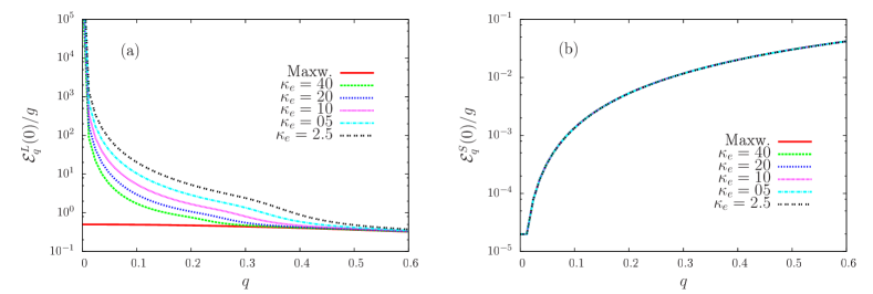
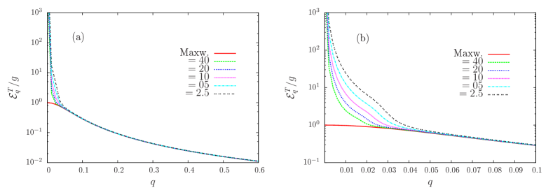
Figure 1: Initial spectrum of electrostatic waves divided by $g$, as a function of normalized wavenumber $q=kv_{e}/\omega_{pe}$, for several values of the index $\kappa_{e}$. The case of Maxwellian distribution, $n_{\kappa e}/n_{e}=0.0$, is also shown for reference. (a) $L$ waves; (b) $S$ waves. For $S$ waves all curves overlap. Electron distribution given by Eq. (2), with $\alpha_{e}=1$ and $u_{\beta,\kappa}^{2}=u_{\beta}^{2}(\kappa_{e}-3/2)/\kappa_{e}$, for $n_{\kappa e}/n_{e}=0.1$. The ion distribution is an isotropic Maxwellian, and $T_{e}/T_{i}=2$. The spectra of $L$ and $S$ waves are given by Eqs. (21) and (25).

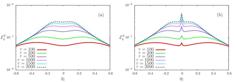
Figure 2: Asymptotic spectrum of $T$ waves, ${\cal E}_{\bf q}^{T}$, characterizing a state of “turbulent equilibrium”, vs normalized wavenumber $q$. (a) ${\cal E}_{\bf q}^{T}$, for $n_{\kappa e}/n_{e}=0.1$, and several values of $\kappa_{e}$. The case of Maxwellian distribution, $n_{\kappa e}/n_{e}=0.0$, is also shown for reference; (b) expanded view of the region of small values of $q$ in Figure 3(a). Other parameters and conditions are as in Figure 3.

Figure 3: (a) 1D spectrum of $T$ waves vs. $q_{\parallel}$, for several values of $\tau$, for $n_{\kappa e}/n_{e}=0.0$; (b) 1D spectrum of $T$ waves vs. $q_{\parallel}$, for several values of $\tau$, for $n_{\kappa e}/n_{e}=5.0\times 10^{-2}$ and $\kappa_{e}=5.0$. Other parameters and conditions are as in Figure 3.

In Figure 3 we show the initial spectrum of electrostatic waves divided by $g$, as a function of normalized wave-number $q=kv_{e}/\omega_{pe}$, for several values of the index $\kappa_{e}$. We assume that the electron population described by a Kappa distribution constitute $10\%$ of the electron population, i.e., $\delta_{e}=0.1$. Figure 3(a) and Figure 3(b) show the initial spectra of $L$ and $S$ waves, obtained using Eqs. (21) and (25), respectively. The spectra obtained in the case of purely Maxwellian distribution, with $n_{\kappa e}/n_{e}=0.0$, are also shown in Figs. 3(a) and 3(b), for reference. In Figs. 3(a) and 3(b) are shown the curves corresponding to several values of $\kappa_{e}$ ($\kappa_{e}=40$, 20, 10, 5, and 2.5).

Figure 3(a) shows that the value of ${\cal E}_{\bf q}^{L}(0)$ in the case of the presence of Kappa population is higher than the value obtained in the case of a purely Maxwellian distribution, with a difference which is already noticeable in the scale of the figure even for the upper limit shown, $q=0.6$, and increases for smaller values of $q$, featuring a peak which diverges for $q\to 0$. For larger values of $\kappa_{e}$, the shape of the $L$ spectrum is similar to the shape exhibited in the case of small values of $\kappa_{e}$, but the magnitude of the spectrum at a given value of $q$ is smaller for increasing values of $\kappa_{e}$. It is noticed, however, that the peak at $q\to 0$ is present even for large values of $\kappa_{e}$.

The presence of the peak in the $L$ spectrum, for $q\to 0$, can be understood by analysis of Eq. (21). In the presence of a population of kappa electrons, even for small value of $n_{\kappa e}/n_{e}$, it is seen that for sufficiently small value of $q$ the contribution due to the Maxwellian population vanishes, due to the factor $\exp\left(-(z_{q}^{L}/q)^{2}/u_{e}^{2}\right)$. For the region of $q$ values where this occurs, the contribution of the Kappa population is dominant, and the equilibrium spectrum can be given by the approximated expression,

$${\cal E}_{\bf q}^{\sigma L}\simeq\frac{g}{2(z_{\bf q}^{L})^{2}}\frac{u_{e,\kappa}^{2}}{u_{e}^{2}}\left(1+\frac{(z_{q}^{L}/q)^{2}}{\kappa_{e}u_{e,\kappa_{e}}^{2}}\right)$$ (32)

In the case of $\kappa_{e}\to\infty$, this expression reduces to $g/(2(z_{\bf q}^{L})^{2}$, which is the expression obtained in the Maxwellian case, as expected. However, for finite values of $\kappa_{e}$, no matter how large, Eq. (32) is seen to diverge at $q\to 0$. The explanation for this is as follows: For large values of $\kappa_{e}$, the Kappa distribution coincides with a Maxwellian distribution, in the region of velocity space with significant electron population. However, the initial spectra of waves is obtained from Eq. (17), which for equilibrium requires balance between the term associated to spontaneous fluctuations, which is proportional to the distribution function, and the term associated to induced emission, which is proportional to the velocity derivative of the distribution function and to the value of the wave spectra at the resonant velocity. For $q\to 0$, the resonant velocity becomes progressively larger. Since for very large velocities the derivative of the Kappa distribution is smaller than the derivative of the Maxwellian distribution, the wave spectra for small $q$ has to be higher in the case of Kappa distribution than in the case of Maxwellian distribution, in order to satisfy the equilibrium condition.

Figure 3(b) shows the values of ${\cal E}_{\bf q}^{S}(0)/g$ vs. $q=kv_{e}/\omega_{pe}$. In fact, the figure shows the values of ${\cal E}_{\bf q}^{S}(0)$ multiplied by $\mu_{\bf q}^{S}$, but we continue to denote the quantity as ${\cal E}_{\bf q}^{S}(0)$, for simplicity. The figure displays the results obtained for several values of $\kappa_{e}$, but the different curves can not be distinguished in the scale of the figure. It is seen that the kappa index of the Kappa distribution is not relevant for the initial spectrum of $S$ waves, while it was seen to be relevant for the initial spectrum of $L$ waves.

We have also obtained the initial spectrum of electrostatic waves by assuming fixed value of the index $\kappa_{e}$ and considering different values of the relative number density of the Kappa population, $n_{\kappa e}/n_{e}$. The results obtained, both for large and small values of $\kappa_{e}$, show that the spectra obtained for $L$ and $S$ waves are almost independent of the value of the number density of the Kappa population, as long it is not zero. These results are not shown here for the sake of economy of space, since the curves obtained for different values of $n_{\kappa e}/n_{e}$ are basically the same as the curves shown in Figure 3, for each value of $\kappa_{e}$. The important point to be emphasized is that the presence of a small population of electrons described by a Kappa population is sufficient to affect significantly the equilibrium spectrum of $L$ waves in the region of small wave numbers, leading to the formation of the peaked feature at $q\simeq 0$.

Figure 3 is dedicated to display the asymptotic spectrum of $T$ waves, obtained using Eq. (31). Figure 3(a) shows ${\cal E}_{\bf q}^{T}/g$ as a function of normalized wavenumber, for $n_{\kappa_{e}}/n_{e}=0.1$, and several values of $\kappa_{e}$, and also present a curve obtained considering a purely Maxwellian electron distribution, obtained with $n_{\kappa e}/n_{e}=0$. The conditions and parameters are the same used to obtain the spectrum of $L$ waves in Figure 3. Let us first comment on the result obtained considering $n_{\kappa_{e}}/n_{e}=0$, given by the red line in Figure 3(a). This result is explained by analysis of Eq (31), which shows that the spectrum of $T$ waves is proportional to the spectrum of $L$ waves, given by Eq. (21), evaluated at $q=q_{m}$. If the Kappa population is vanishing, $n_{\kappa_{e}}/n_{e}=0$, the Kappa contributions vanishes in Eq. (21), and the contributions due to the Maxwellian population in the numerator and in the denominator cancel out, and the spectrum turns out to be given by

$${\cal E}_{\bf q}^{\sigma T}\simeq 2\frac{g}{2(z_{{\bf q}_{m}}^{L})^{2}}=\frac{g}{2+3q_{m}^{2}}.$$

At $q=0$, the amplitude of the spectrum of $T$ waves in the case of Maxwellian electron distribution is therefore twice the magnitude of the spectrum of $L$ waves, but decays faster for larger values of $q$, since $q_{m}>>q$. With the presence of a population described by a Kappa distribution, Figure 3(a) shows that the spectrum of $T$ waves is modified in the region of small wave numbers, in comparison with the spectrum obtained in the Maxwellian case. In the scale of the figure, the modification is noticeable for normalized wave-number $q<0.1$, with a difference that increases with the decrease of the $\kappa_{e}$ index, i.e., increases with the increase of the non-thermal character of the electron distribution. The spectrum features divergent behavior for $q\to 0$, as already noticed for the $L$ waves in Figure 3.

Figure 3(b) shows an expanded view of the region of small values of $q$, for the conditions which have been discussed in Figure 3(a). The expanded view clearly shows the increase of the magnitude of the $T$ wave spectrum at small values of $q$. For instance, it is seen that for $q\simeq 0.02$ the intensity of the spectrum of $T$ waves in the case of $\kappa_{e}=2.5$ is about one order of magnitude above the intensity displayed in the case of $\kappa_{e}=40$.

We have also investigated the dependence of the $T$ spectrum on the relative number density $n_{\kappa e}/n_{e}$, for a fixed value of $\kappa_{e}$. The results obtained have shown that the $T$ wave spectrum obtained in the presence of a Kappa distribution is almost independent of the number density of the Kappa population. The only noticeable feature in the spectra is the presence of the peak around $q=0$, which occurs for any finite value of $n_{\kappa e}/n_{e}$, and vanishes in the purely Maxwellian case ($n_{\kappa e}/n_{e}=0$).

In addition to these results concerning the initial spectra of electrostatic waves and the asymptotic spectrum of transverse waves, we also present some results which show the time evolution of the wave-particle system, comparing a situation in which the background electron velocity distribution is a Maxwellian distribution with a situation in which an “halo” population described by as isotropic Kappa distribution is also present.

For the study of the time evolution of the system, we utilize the set of weak turbulence equations, with some additional approximations. Regarding to the plasma particles, we assume that the ion velocity distribution remains constant along the evolution, and that in the case of the equation for the electron distribution the quasilinear diffusion due to $S$ waves can be neglected in comparison with the diffusion caused by the $L$ waves. Regarding the waves, we describe the evolution of the $L$ waves by including the spontaneous and induced emission processes, the three-wave decay processes involving $L$ and $S$ waves, and the scattering process involving two $L$ waves and the particles. Nonlinear interaction involving $T$ waves are neglected in the equation for the time evolution of the $L$ waves, for simplicity, which is common practice in the literature. The evolution of $S$ waves is described in the present analysis by taking into account the emission terms and the three-wave decay term involving $L$ and $S$ waves, and neglecting the effect of the decay term involving $S$, $L$ and $T$ waves, and also the scattering term. In the equation for the $T$ waves, however, which contains only nonlinear effects, we keep all the terms which have already been described in the introduction section, namely, the decay involving a $T$ wave and two $L$ waves, the decay involving a $T$ wave, a $L$ wave and a $S$ wave, the decay involving two $T$ waves and a $L$ wave, and the scattering term.

We utilize a two-dimensional approximation (2D), considering a grid of 51$\times$ 101 points in ($u_{\perp},u_{z}$) space, with $0\leq u_{\perp}\leq 12$ and $-12\leq u_{z}\leq 12$, a grid of $51\times 51$ points in $(q_{\perp},q_{z})$ space for $L$ and $S$ waves, and a grid of $71\times 71$ points in $(q_{\perp},q_{z}$) space for the $T$ waves, which develop fine features which require better resolution than the $L$ and $S$ waves, considering for all waves the evolution in the interval $0\leq q_{\perp}\leq 0.6$ and $0\leq q_{z}\leq 0.6$. The normalized time step has been adopted as $\Delta\tau=0.1$, and the equations were solved using a fourth-order Runge-Kutta procedure for the wave equations and the splitting method for the equation describing the time evolution of the electrons.

As starting conditions, we assume that the background electron population is described by distribution function (2), with the 2D versions of Eqs. (4) and (4), with the Kappa distribution defined using $\alpha=1$ and $u_{e,\kappa}^{2}=u_{e}^{2}(\kappa_{e}-1)/\kappa_{e}$, which is the proper value of $u_{e,\kappa}^{2}$ for 2D distributions. We assume that the ion distribution is described by an isotropic Maxwellian distribution, with $T_{e}/T_{i}=2$. We also assume that the plasma parameter is $(n\lambda_{D}^{3})^{-1}=5.0\times 10^{-3}$, and $v_{e}^{2}/c^{2}=4.0\times 10^{-3}$, values which have already been used in analyses of the plasma emission without taking into account the presence of a Kappa distribution Ziebell et al. (2014b, c).

A further approximation is made for the numerical analysis, regarding the initial wave spectra. As already discussed in the initial paragraphs of this section on numerical results (see equation (32) and the accompanying comments), in the presence of a Kappa distribution the initial spectrum of $L$ diverges for $q\to 0$. This divergence, although consistent with the non-relativistic approach, is not appropriate for the numerical analysis. In our numerical implementation of the formalism, the initial spectrum of $L$ waves is given by equation (21) down to the value of $q$ such the resonant velocity becomes equal to $c$, i.e., the value of $q$ for which $z_{q}^{L}/q=c/v_{e}$. It is assumed that for values of $q$ smaller than this value, the initial $L$ wave spectrum is given by the same value obtained at the limit value of the resonant $q$. With such approximation, when a Kappa distribution is assumed to be present, the initial spectrum of $L$ has significant growth in the region of small values of $q$, in comparison with the spectrum in the case of a Maxwellian plasma background, but the divergence is avoided. The initial spectrum of $L$ waves is therefore given by equation (21), with an approximation in the region of small values of $q$, and the spectrum of $S$ is given by equation (25). The $T$ waves are assumed not present at initial time.

Figure 3 shows one dimensional (1D) representations of the spectrum of $T$ waves, i.e., obtained after integration of ${\cal E}_{\bf q}^{T}$ along the perpendicular component of normalized wavenumber, $q_{\perp}$. The spectra are shown for different values of $\tau$, and show the evolution of the $T$ wave spectrum. Figure 3(a) displays the wave spectra obtained in the case of purely Maxwellian electron distribution, i.e., $n_{\kappa e}/n_{e}=0.0$. Figure 3(b) depicts the wave spectra obtained when the electron distribution contains a Kappa population, with $n_{\kappa e}/n_{e}=5.0\times 10^{-2}$, and $\kappa_{e}=5.0$. In panel (a), it is seem that the amplitude of the waves increases for all values of $q_{z}$, and gradually evolves toward the asymptotic solution described by equation (31) in the case of $n_{\kappa e}=0.0$, and which appears as the red lines in Figure 3. The situation depicted in Figure 3(a) corresponds to the initial stages of the evolution, which is displayed up to longer time in Figure 2 of Ref. Ziebell et al. (2014b). In the presence of a small Kappa population, the spectrum of $T$ waves evolves as shown in Figure 3(b). The spectrum grows for all values of $q_{z}$, much as seen in Figure 3(a), but there is difference. A peak is seen to appear near $q_{z}=0$, and grows in time. What is seen is Figure 3(b) are some steps in the time evolution of the spectrum which is asymptotically given by equation (31), and represented in Figure 3. It must be noticed that the peak near $q_{z}=0$ in Figure 3(b) has a finite height. It does not diverge as the peaks appearing in Figure 3, because for the numerical analysis of the equation which describe the time evolution we have assumed that the $L$ wave spectrum saturates for sufficiently small value of $q$, instead of growing infinitely for $q\to 0$.

The growth of the peak near $q=0$ in the $T$ wave spectrum can be explained as follows. The dominant process for the formation of background spectrum of $T$ is the scattering involving $L$ waves. The scattering effect is maximum for wave lengths which satisfy $z_{q}^{T}=z_{q^{\prime}}^{L}$, which means $q^{\prime}=q_{m}$, where $q_{m}$ is defined by equation (31). As seen in Figure 3(a), in the case of a small population described by a Kappa distribution the spectrum of $L$ waves is above the spectra obtained in the purely Maxwellian case for $q^{\prime}\leq 0.2$. The scattering process is therefore most effective to generate $T$ waves with $q\leq 0.02$, for the value of $v_{e}/c$ which we have assumed. The scattering of $L$ waves is the main responsible for the formation of the spectrum of $T$ waves, and the peak for large wavelengths which is seen in the $L$ wave spectrum which occurs in the presence of Kappa distributed electrons is the cause for the growth of the peak for large wavelength in the $T$ wave spectrum.

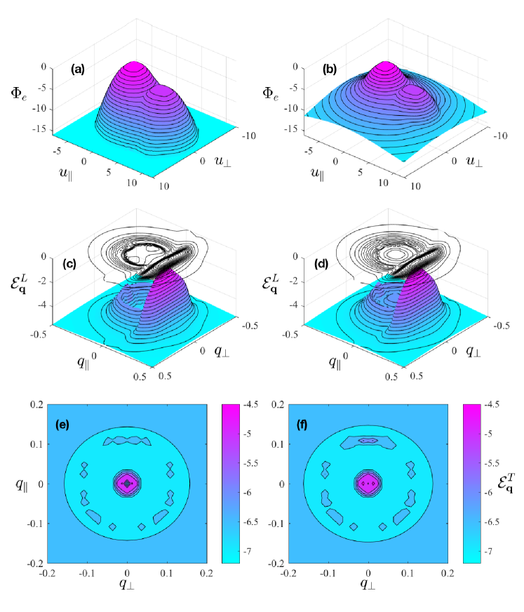
Figure 4: (a) Electron distribution function at $\tau=500$, vs. $u_{\parallel}$ and $u_{\perp}$, for $n_{\kappa e}/n_{e}=0.0$; (b) Electron distribution function at $\tau=500$, vs. $u_{\parallel}$ and $u_{\perp}$, for $n_{\kappa e}/n_{e}=5.0\times 10^{-2}$; (c) Spectrum of $L$ waves at $\tau=500$, vs. $q_{\parallel}$ and $q_{\perp}$, for $n_{\kappa e}/n_{e}=0.0$; (d) Spectrum of $L$ waves at $\tau=500$, vs. $q_{\parallel}$ and $q_{\perp}$, for $n_{\kappa e}/n_{e}=5.0\times 10^{-2}$; (e) Spectrum of $T$ waves at $\tau=500$, vs. $q_{\parallel}$ and $q_{\perp}$, for $n_{\kappa e}/n_{e}=0.0$; (f) Spectrum of $T$ waves at $\tau=500$, vs. $q_{\parallel}$ and $q_{\perp}$, for $n_{\kappa e}/n_{e}=5.0\times 10^{-2}$. Input parameters are as follows: $T_{e}/T_{i}=2.0$, $T_{b}/T_{e}=1.0$, $n_{b}/n_{e}=1.0\times 10^{-3}$, $v_{b}/v_{e}=6.0$, $g=5.0\times 10^{-3}$, $\kappa_{e}=5.0$.

In what follows, we investigate the time evolution of the beam-plasma instability, comparing the situation in which the background electron distribution is purely Maxwellian with a case in which there is also an “halo” population described by a Kappa distribution. We assume a beam population described by a displaced Maxwellian distribution, with normalized beam velocity $u_{b}=6.0$, number density given by $n_{b}/n_{e}=1.0\times 10^{-3}$, and temperature $T_{b}=T_{e}$, Figure 4 shows 2D plots of the electron velocity distribution. Due to the presence of the beam, the background electron distribution is slightly displaced in velocity space, so that the average velocity of the complete electron velocity distribution is zero.

Figure 4 shows 2D plots of the electron velocity distribution, the spectrum of $L$ waves, and the spectrum of $T$ waves, at $\tau=500$. The spectrum of $S$ waves remain very similar to the initial shape, and is not shown. The three panels at the left column were obtained considering that the background electron distribution is a Maxwellian distribution, i.e., considering $n_{\kappa e}/n_{e}=0.0$, and the panels at the right column were obtained assuming $n_{\kappa e}/n_{e}=0.05$, with $\kappa_{e}=5.0$. For the parameters chosen, at such a point in the time evolution the quasilinear process has already transferred to waves a significant part of the energy available in the beam, creating a peak in the spectrum of $L$ waves. The nonlinear processes are already operative, creating a ring-like structure in the spectrum of $L$ waves, creating a spectrum of $T$ waves over the whole grid of $q$ values, and creating some peaked features for the $T$ waves, in the region of small values of $q$. The situations depicted in Figures 4(a), (c) and (e) correspond to those appearing in Figures 1(b), 2(b) and 4(b) of Ref. Ziebell et al. (2015), which is dedicated to the study of emission by nonlinear processes in a plasma with Maxwellian background distributions. It can be noticed in Figures 4(a) and 4(b) that the region between the core of the velocity distribution and the peak of the beam distribution is already quite flattened, corresponding to the formation of the peak in the $L$ spectrum which is centered at $(q_{\perp},q_{z})\simeq(0,0.2)$ in Figures 4(c) and 4(d).

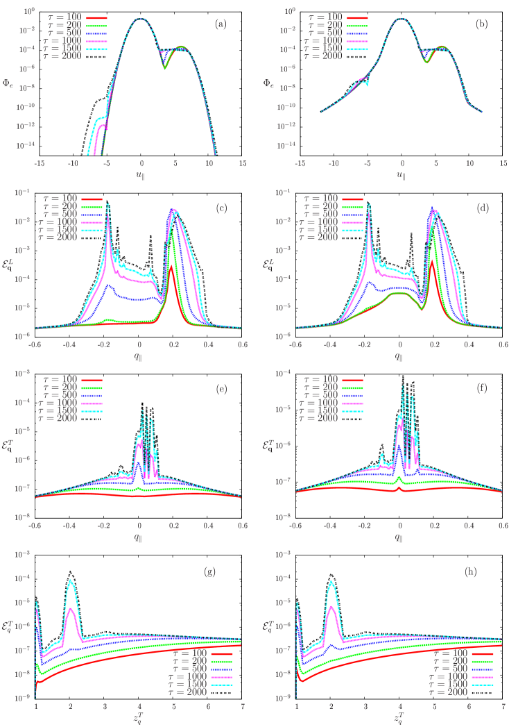
Figure 5: (a) 1D electron distribution function vs. $u_{\parallel}$, for several values of $\tau$, for $n_{\kappa e}/n_{e}=0.0$; (b) 1D electron distribution function vs. $u_{\parallel}$. for several values of $\tau=500$, for $n_{\kappa e}/n_{e}=5.0\times 10^{-2}$; (c) 1D spectrum of $L$ waves vs. $q_{\parallel}$, for several values of $\tau$, for $n_{\kappa e}/n_{e}=0.0$; (d) 1D spectrum of $L$ waves vs. $q_{\parallel}$, for several values of $\tau$, for $n_{\kappa e}/n_{e}=5.0\times 10^{-2}$; (e) 1D spectrum of $T$ waves vs. $q_{\parallel}$, for several values of $\tau$, for $n_{\kappa e}/n_{e}=0.0$; (f) 1D spectrum of $T$ waves vs. $q_{\parallel}$, for several values of $\tau$, for $n_{\kappa e}/n_{e}=5.0\times 10^{-2}$. (g) Spectrum of $T$ waves vs. $q$, for several values of $\tau$, for $n_{\kappa e}/n_{e}=0.0$; (h) Spectrum of $T$ waves vs. $q$, for several values of $\tau$, for $n_{\kappa e}/n_{e}=5.0\times 10^{-2}$. The parameters are the same used in Figure 4.

The results appearing in Figure 4 can be considered as representative of the time evolution of the wave-particle system. For further analysis of the time evolution, we show in Figure 5 1D representations of the electron distribution and of the wave spectra, obtained after integration of the 2D quantities, along $u_{\perp}$ in the case of the velocity distribution and along $q_{\perp}$ in the case of the wave spectra. As in Figure 4, the left column displays results obtained assuming $n_{\kappa e}/n_{e}=0.0$, and the right column shows results obtained assuming $n_{\kappa e}/n_{e}=0.05$, with $\kappa_{e}=5.0$. The electron distribution function in each case is shown in Figures 5(a) and 5(b), respectively, for several values of $\tau$, between $\tau=100$ and $\tau=2000$. In both panels, it can be noticed the gradual flattening of the peak of the beam distribution, and the formation of a plateau in the region of velocities between the beam and the core distribution. In Figure 5(a), it is also noticed the appearing of a small population of backscattered electrons, which start to become distinguishable at $\tau\simeq 1000$. In panel 5(b), these backscattered electrons are not noticeable in the scale of the figure, because the Kappa distribution already had a sizeable population at that region of velocity space.

Figures 5(c) and 5(d) show a 1D projection of the $L$ wave spectrum. In panel (c), one notices that at $\tau=100$ the only distinctive feature in the spectrum is the primary peak generated at $q_{z}\simeq 0.2$, at the spectral region where the waves are in resonance with electrons in the region of positive velocity in the velocity distribution. At $\tau=200$, there is already a hint of a backward peak, at $q_{z}\simeq-0.2$. At $\tau=500$, and beyond that, the backward peak appears well developed, and there is a profile in the wave spectrum, continuous between the forward peak and the backward peak. This is only a 1D projection of the ring formed by scattering and decay, which is seen in the 2D representation appearing in Figure 4(c). On the other hand, when the electron distribution function features the presence of a Kappa distribution, the $L$ wave spectrum at $\tau=100$ features the peak generated by quasilinear effect at $q_{z}\simeq 0.2$, and also the peak around $q=0$, characteristic of the spectrum at equilibrium in the presence of a Kappa distribution. Due to the approximation which we have adopted, of a limiting resonant velocity, the spectrum at $q=0$ is finite instead of divergent. The 1D projection at Figure 5(d) shows at $\tau=200$ already a hint of the backward peak. At $\tau=500$, and beyond, the 1D spectrum of Figure 5(d) becomes similar to that appearing at Figure 5(c), but this is only the effect of the 1D projection. The actual spectrum in the case of Figure 5(d) is constituted by the primary and the back-scattered peaks, by the peak around $q=0$, and by the ring structure formed by nonlinear effects, as seen in Figure 4(d).

The 1D projection of the spectrum of $T$ waves appears depicted in Figures 5(e) and 5(f), for several values of $\tau$. In both panels the sequence of lines show initially the formation of a background spectrum of $T$ waves, added of the growth of a wave peak around $q_{z}=0$. Between $\tau=500$ and $\tau=1000$, other peaked structures appear in the 1D representations of Figures 5(e,f), which are projections of the narrow ring structure seen in Figures 4(e) and 4(f). The 1D representations in Figure 5, as well as the 2D representations in Figure 4, show that the $T$ wave spectrum obtained in the case of Maxwellian electron distribution is very similar to the $T$ wave spectrum obtained in the case of the presence of a “halo” described by a Kappa distribution. The only noticeable difference is that the peaks appearing in the $T$ wave spectrum are slightly higher in the case of $n_{\kappa e}\neq 0$, panel (e), than in the case of $n_{\kappa e}=0$, panel (f), for the same value of $\tau$.

Another representation of the $T$ wave spectrum appears in Figures 5(g) and 5(h), which display the spectrum of $T$ waves after integration along pitch angle. That is, Figures 5(g) and 5(h) show the quantity

$${\cal E}_{q}=\int_{0}^{2\pi}d\theta\;q{\cal E}_{\bf q}^{T}$$

as a function of the normalized wave frequency. This representation clearly shows the early formation of the $T$ wave background, then the onset of the primary peak of fundamental emission, with frequency equal to the electron plasma frequency, and later on the onset of harmonic emission, with the peak of emission at $2\omega_{pe}$ clearly emerging between $\tau=500$ and $\tau=1000$. The comparison between Figure 5(h) and Figure 5(g) show that the curves obtained in both cases are qualitatively the same, with the sole difference that the peaks are slightly higher in the case of $n_{\kappa e}\neq 0$, shown in Figure 5(h).

VI Final remarks

In the present paper we have discussed the spectra of electrostatic and electromagnetic waves which may be present at quiescent situation in plasmas whose particles have velocity distribution functions which are a combination of a thermal background and an energetic “halo” distribution. The motivation for the study has been the abundance of measurements made in the solar wind environment, by satellites at different orbits, which show the occurrence of particle distribution functions with these characteristics. For the analysis presented in the paper, the electron velocity distribution has been represented as a summation of a Maxwellian distribution function and an isotropic Kappa distribution, with the fraction of population having the Kappa populations assumed as a free parameter.

The investigation has been conducted using the theoretical framework of weak turbulence theory. We have briefly discussed basic features of the equations of weak turbulence theory, and we have initially used these equations to obtain expressions for the spectra of electrostatic waves, obtained as the outcome of the balance between spontaneous fluctuations and induced emission. These equilibrium spectra, for high frequency Langmuir waves ($L$) and for low frequency ion-acoustic waves ($S$), have been routinely discussed in the literature for the case of Maxwellian plasmas, but the present paper presents as a novel feature a description of the effects of the presence of a population of particles described by a Kappa velocity distribution. Theoretical expressions for the spectra of L and S waves have been obtained considering that both ions and electrons can be described by a combination of Maxwellian and Kappa distribution. Some numerical results have also been presented, considering the case of Maxwellian distribution for the ions and the combined distribution for electrons, and considering different values of the $\kappa_{e}$ index. These results show that the effect of the presence of the Kappa distribution is noticeable in the spectrum of $L$ waves in the region of large wavelengths, with difference relative to the spectrum obtained in the case of purely Maxwellian distribution which increases for decreasing values of the index $\kappa_{e}$ in the energetic population. The distinctive feature, which exists even for very tenuous Kappa population, is the presence of a peak of wave intensity for very large wavelengths (wave-number $k\to 0$).

We have also discussed the characteristics of the spectrum of electromagnetic waves ($T$), which shall be present in the plasma as the outcome of nonlinear processes involving $L$ and $S$ waves, and particles. These spectra can be characterized as a state of “turbulent equilibrium”. The turbulent equilibrium spectra have already been discussed for the case of Maxwellian velocity distributions, and the present paper extends the discussion for the case in which an energetic “halo” described as a Kappa distribution is also present in the plasma. The results obtained show that the spectrum of $T$ waves has the general features similar to those obtained in the case of Maxwellian distributions, with the effect of the presence of the Kappa population appearing as a peak of $T$ waves in the large wavelength region, much narrower than the peak obtained in the spectrum of the $L$ waves.

In addition to the results concerning the equilibrium spectra, we have also presented some results which show the time evolution of the spectra of $L$ and $T$ waves, and the time evolution of the electron distribution function, as a result of the presence of a tenuous electron beam travelling in the plasma. We have followed the time evolution of the wave-particle system up to the formation of the plateau in the electron distribution function which indicates the saturation of the induced processes described by quasilinear theory. The results which were shown in the paper compare the results obtained in the case in which the background electron population is described by a Maxwellian distribution, with results obtained in the case of a background distribution described as a core population with Maxwellian distribution and a tenuous population with isotropic Kappa distribution. It was shown that the time evolution of the spectrum of $L$ waves obtained in the presence of the “halo” distribution is qualitatively very similar to the spectrum obtained in the case of thermal background distribution, except for the occurrence of the enhanced wave intensity for $k\to 0$, characteristic of the presence of a Kappa population of particles. The spectra obtained for the $T$ waves along the time evolution, in the two situations which have been considered, are also qualitatively very similar, with the difference that the peak corresponding to the harmonic emission is slightly more pronounced in the presence of a tenuous Kappa distribution, in comparison with harmonic emission obtained in the case of Maxwellian background population.