Heavy quark radiation in NLO+PS POWHEG generators

Abstract

In this paper we deal with radiation from heavy quarks in the context of next-to-leading order calculations matched to parton shower generators. A new algorithm for radiation from massive quarks is presented that has considerable advantages over the one previously employed. We implement the algorithm in the framework of the POWHEG-BOX, and compare it with the previous one in the case of the hvq generator for bottom production in hadronic collisions, and in the case of the bb4l generator for top production and decay.

1 Introduction

The production and detection of bottom quarks play an important rôle in various contexts in LHC physics. Letting aside the very abundant direct production, that is exploited for flavour physics studies, bottom is used to identify top particles and to study their properties. Furthermore, it is the dominant decay mode of the Higgs boson, that can be used to study processes as the associate $HV$ production Aaboud:2017xsd ; CMS:2017tkf and the large transverse momentum production CMS:2017cbv . In searches for physics beyond the Standard Model, bottom also appears often produced in association with new-physics objects.

Having a mass much larger than the typical hadronic scales, bottom quark production is calculable in perturbative QCD. In cases when the transverse momentum involved in the production is large compared to its mass, as, for example, in high-energy $e^{+}e^{-}$ annihilation, or in production at large transverse momentum in hadronic collisions, bottom can behave as a light parton, and give rise to a hadronic jet. Techniques for dealing with these regimes have been developed in the past Cacciari:1998it , and have been applied to the LHC case Cacciari:2012ny . They allow for the computation of the transverse momentum spectrum of promptly produced $b$ quarks at next-to-leading order in QCD, including the resummation of large logarithms of the ratio of the transverse momentum over the bottom mass up to next-to-leading-logarithmic accuracy. These large logarithms can arise both from initial state radiation, when, for instance, an incoming gluon splits into a $b\bar{b}$ pair, with one of the $b$ undergoing a large-momentum-transfer collision with a parton from the target, and from final state radiation. In the last case, an outgoing gluon can split into a $b\bar{b}$ pair, or a directly produced $b$ quark can emit a collinear gluon.

The large transverse momentum regime is treated consistently at the leading logarithmic level in parton shower generators. At the most basic level, heavy flavours are treated as light flavours, but with a shower cut-off scale of the order of the heavy quark mass. However, considerable work has been performed to better account for mass effects. In some generators, this is achieved by suitable modifications of the splitting kinematics and splitting kernels Sjostrand:2014zea ; Bellm:2017bvx . The Sherpa dipole shower Schumann:2007mg makes use of the Catani-Seymour dipoles for massive quarks Catani:2002hc . The Catani-Seymour formalism is also used in the DIRE shower Hoche:2015sya . In ref. GehrmannDeRidder:2011dm a final state dipole-antenna shower for massive fermions is proposed, based upon the corresponding antenna subtraction formalism of ref. GehrmannDeRidder:2009fz .

In next-to-leading order (NLO) calculations matched to Shower generators (NLO+PS) for heavy flavour production Frixione:2003ei ; Frixione:2007nw , one generally treats the heavy flavour as being very heavy. The heavy quark mass thus acts as a cut-off on collinear singularities, that are thus not resummed. This approach has in fact proven to be quite viable in heavy flavour production even at relatively large momentum transfer Cacciari:2012ny . Consider, for example, heavy quark pair production in a POWHEG framework. By neglecting collinear singularities from heavy quarks, the only singular region that we have to consider has to do with initial state radiation involving only light partons. Since the POWHEG procedure guarantees that the matrix elements are given correctly for up to one hard radiation, gluon splitting, flavour excitation and radiation from the heavy flavour are included, so that the logarithmically enhanced terms are correctly reproduced at first order. Higher order leading logarithms, however, are not treated correctly. In particular, there are reasons to give an adequate treatment to final state radiation from a high transverse momentum bottom quark. In fact, this radiation process is intimately related to the physics of the bottom fragmentation function, and may have important effects in processes of considerable interest, like for example in top decay.

In the POWHEG-BOX framework, a facility for the treatment of collinear radiation from a heavy particle was set up in ref. Barze:2012tt , in the framework of electroweak corrections to $W$ production. In that context, the purpose was to deal with mass effects in the final state radiation of photon from the lepton in $W$ decays. The same framework is also appropriate for describing radiation from heavy quarks. In particular, it was adopted in refs. Campbell:2014kua , where the ttb_NLO_dec generator was introduced, and in refs. Jezo:2016ujg for the b_bbar_4l generator, for dealing with radiation from bottom quarks in top decays.

The purpose of the present paper is twofold: we present a new algorithm for radiation from a heavy quark, that has proven superior to the old one; furthermore we perform a thorough investigation of the behaviour of this component of the POWHEG generator, also by comparing the two methods, both in the framework of bottom quarks generated in top decay, and in inclusive bottom quark pair production. In the last case, such a study was never carried out.

The paper is organized as follows: in section 2 we describe the new algorithm, in section 3 we illustrate our phenomenological studies, and in section 4 we give our conclusions.

2 Description of the new algorithm

2.1 The POWHEG mapping for the massive emitter case

Let us assume for definiteness to deal with a scattering process involving $n$ partons in the final state at lowest order in perturbation theory. The generic point in the corresponding Born phase space, referred also as Born configuration, will be denoted with barred momenta

$$\overline{\Phi}_{n}=\{\overline{k}_{1},\dots,\overline{k}_{n}\}.$$ (1)

The corresponding phase space volume element is given by

$$\mathrm{d}\overline{\Phi}_{n}=\prod_{i=1}^{n}\frac{\mathrm{d}^{3}\vec{\overline{k}}_{i}}{(2\pi)^{3}2\overline{k}_{i}^{0}}(2\pi)^{4}\delta^{(4)}\left(q-\sum_{i=1}^{n}\overline{k}_{i}\right),$$ (2)

where $q$ is the total incoming 4-momentum. At Next-to-Leading order (NLO), one must also include processes of emission of one more real massless extra parton, resulting in a $n+1$-body kinematics which we will denote as

$$\Phi_{n}=\{k_{1},\dots,k_{n+1}\}.$$ (3)

The singular regions of the real phase space are separated by means of suitable projection operators; in each of them, the radiated parton phase space is parametrised in terms of the FKS variables Frixione:1995ms (the notations $\vec{p}$ and $\underline{p}$ for a generic momentum $p$ denote the tri-impulse and its modulus respectively)

$$\xi=\frac{2\underline{k}_{n+1}}{q^{0}},\quad y=\frac{\vec{k}_{n}\cdot\vec{k}_{n+1}}{\underline{k}_{n}\underline{k}_{n+1}},$$ (4)

as shown in Fig. 1, where we have assumed that the emitter and the FKS partons are respectively the $n$-th and the $n+1$-th parton. The rescaled energy $\xi$ is related to the soft limit ($\xi\to 0$), and the variable $y$ to the collinear one ($y\to\pm 1$). The definition of the azimuthal angle $\phi$, in the POWHEG framework, departs from the standard FKS definition. It is taken as the polar angle of the splitting around the axis parallel to the momentum of the recoil system, in the rest frame where $q=(q^{0},\vec{0})$.

Figure 1: Kinematics for a real configuration: $k_{n}$ is the massive emitter, $k_{n+1}$ is the radiated parton. $y$ denotes the cosine of the angle between the two tri-vectors.

In what follows, we will construct a one-to-one map from a real configuration with radiation variables $(\xi,y,\phi)$ into a Born one. This leads to a factorisation of the real phase space in term of Born and radiation variables.

The mapping can be reduced to the case of the map from a 3-body phase space into a 2-body one. Inserting into the $(n+1)$-body phase space volume element the identities

$$1=\int\mathrm{d}^{4}k_{\text{rec}}\delta^{(4)}\left(k_{\text{rec}}-\sum_{i=1}^{n-1}k_{i}\right)$$ (5)

and

$$1=\int\mathrm{d}M^{2}_{\text{rec}}\delta(M^{2}_{\text{rec}}-k_{rec}^{2}),$$ (6)

the phase space is decomposed into a chain of two consecutive processes. With reference to Fig. 1, they are: the decay of a particle with momentum $q$ into the 3-body system formed by the emitter $k_{n}$, the FKS-parton $k_{n+1}$ and the “recoil” system, with momentum and invariant mass

$$k_{\text{rec}}=\sum_{i=1}^{n-1}k_{i}=q-k_{n}-k_{n+1},\quad M_{\text{rec}}^{2}=k_{\text{rec}}^{2},$$ (7)

followed by the decay of the latter into the other $n-1$ particles. In formula, we have

$$\mathrm{d}\Phi_{n+1}=\mathrm{d}\Phi_{3}\mathrm{d}\Phi_{\text{rec}},$$ (8)

where

$$\begin{split}\mathrm{d}\Phi_{3}=&\frac{\mathrm{d}M^{2}_{\text{rec}}}{2\pi}\frac{\mathrm{d}^{3}\vec{k}_{n}}{2k^{0}_{n}(2\pi)^{3}}\frac{\mathrm{d}^{3}\vec{k}_{n+1}}{2k^{0}_{n+1}(2\pi)^{3}}\frac{\mathrm{d}^{3}\vec{k}_{\text{rec}}}{2k^{0}_{\text{rec}}(2\pi)^{3}}\\ &\times(2\pi)^{4}\delta^{(4)}(q-k_{n}-k_{n+1}-k_{\text{rec}}),\end{split}$$ (9)

$$\mathrm{d}\Phi_{\text{rec}}=\prod_{i=1}^{n-1}\frac{\mathrm{d}^{3}\vec{k}_{i}}{2k_{i}^{0}(2\pi)^{3}}(2\pi)^{4}\delta^{(4)}\left(k_{\text{rec}}-\sum_{i=1}^{n-1}k_{i}\right).$$ (10)

We now focus on the 3-body process; under the action of the mapping, the $k_{n}$ and $k_{n+1}$ partons will be replaced by a single parton with mass $m$ and momentum $\overline{k}_{n}$. We define

$$k\equiv k_{n}+k_{n+1},$$ (11)

so that

$$k_{\text{rec}}=q-k\implies k^{0}_{\text{rec}}=q^{0}-k^{0},\vec{k}_{\text{rec}}=-\vec{k}.$$ (12)

We fix the transformation by demanding $\vec{\overline{k}}_{n}\parallel\vec{k}$. Care must be taken to ensure the conservation of energy-momentum also for the resulting Born configuration. This is accomplished by performing a boost $\Lambda$ in the direction $\vec{k}$ and defining

$$\overline{k}_{n}=q-\Lambda k_{\text{rec}},$$ (13)

We determine the velocity parameter $\beta$ of the boost transformation from the mass-shell condition

$$\overline{k}_{n}^{2}=(q-\Lambda k_{\text{rec}})^{2}=m^{2}.$$ (14)

We get

$$\begin{split}\beta&=\frac{-4\underline{k}_{\text{rec}}k^{0}_{\text{rec}}q^{2}}{(q^{2}-m^{2}+M_{\text{rec}}^{2})^{2}+4\underline{k}_{\text{rec}}^{2}q^{2}}\\ &\hskip 14.22636pt+\frac{(q^{2}-m^{2}+M_{\text{rec}}^{2})\sqrt{(q^{2}-m^{2}+M_{\text{rec}}^{2})^{2}-4M_{\text{rec}}^{2}q^{2}}}{(q^{2}-m^{2}+M_{\text{rec}}^{2})^{2}+4\underline{k}_{\text{rec}}^{2}q^{2}}.\end{split}$$ (15)

We define the other barred variables as

$$\overline{k}_{i}=\Lambda k_{i},\quad i=1,\dots,n-1.$$ (16)

Their mass relations are preserved by the boost transformation and, furthermore, we have

$$\begin{split}\sum_{i=1}^{n}\overline{k}_{i}&=\sum_{i=1}^{n-1}\overline{k}_{i}+\overline{k}_{n}=q+\sum_{i=1}^{n-1}\Lambda k_{i}-\Lambda k_{\text{rec}}\\ &=q+\Lambda\bigg{(}\sum_{i}^{n-1}k_{i}-k_{\text{rec}}\bigg{)}=q,\end{split}$$ (17)

which is the energy-momentum conservation for the Born configuration.

2.2 Inverse map

We now detail the construction of the inverse map, which is what is actually needed in the applications. Suppose that a Born event has been generated, i.e. the barred variables $\overline{k}_{i}$ ($i=1,\cdots,n$) are given. Then, $M_{\text{rec}}^{2}$ is obtained inverting eq. (13):

$$M_{\text{rec}}^{2}=(\Lambda k_{\text{rec}})^{2}=(q-\overline{k}_{n})^{2}=q^{2}+m^{2}-2q^{0}\overline{k}_{n}^{0}.$$ (18)

We want to attach to it a radiation described by the radiation variables $\xi$, $y$ and $\phi$. For future convenience we introduce the largest allowed value for $\xi$

$$\xi_{\rm max}\equiv 1-\frac{(m+M_{\rm rec})^{2}}{q^{2}}.$$ (19)

The energy of the radiated parton is

$$k^{0}_{n+1}=\underline{k}_{n+1}=\frac{q^{0}}{2}\xi.$$ (20)

Energy conservation requires that

$$q^{0}=k^{0}_{n+1}+\sqrt{\underline{k}_{n}^{2}+m^{2}}+\sqrt{\underline{k}_{\rm rec}^{2}+M_{\text{rec}}^{2}},$$ (21)

where

$$\underline{k}_{\rm rec}^{2}=\underline{k}_{n}^{2}+\underline{k}_{n+1}^{2}+2\underline{k}_{n}\underline{k}_{n+1}y.$$ (22)

We can solve equation (21) for $\underline{k}_{n}$ in a standard way, by bringing in turn each single square root on one side of the equation and squaring both sides. By doing this we actually find the solutions of all of the following equations

$$q^{0}=k^{0}_{n+1}\pm\sqrt{\underline{k}_{n}^{2}+m^{2}}\pm\sqrt{\underline{k}_{\rm rec}^{2}+M_{\text{rec}}^{2}},$$ (23)

for all possible combinations of the signs in front of the square root. The solutions are given by

$$\begin{split}\underline{k}_{n}^{(\pm)}&=\frac{-(2\overline{k}_{n}^{0}-q^{0}\xi)\xi y}{(2-\xi)^{2}-\xi^{2}y^{2}}\\ &\pm\frac{(2-\xi)\sqrt{(2\overline{k}_{n}^{0}-q^{0}\xi)^{2}-m^{2}\xi^{2}(1-y^{2})-4m^{2}(1-\xi)}}{(2-\xi)^{2}-\xi^{2}y^{2}}.\end{split}$$ (24)

In order for them to exist, the argument of the square root must be positive. This leads to the bound

$$(q^{2}-m^{2}+m^{2}y^{2})\xi^{2}-4(q^{0}\overline{k}_{n}^{0}-m^{2})\xi+4\overline{\underline{k}}_{n}^{2}>0,$$ (25)

with $\overline{\underline{k}}_{n}^{2}=(\overline{k}_{n}^{0})^{2}-m^{2}$. Eq.(25) is satisfied if either $\xi>\xi^{(+)}(y)$ or $\xi<\xi^{(-)}(y)$, with

$$\xi^{(\pm)}(y) = 2\frac{\overline{k}_{n}^{0}q^{0}-m^{2}\pm m\sqrt{(q^{0}-\overline{k}_{n}^{0})^{2}-\overline{\underline{k}}_{n}^{2}y^{2}}}{q^{2}-m^{2}+m^{2}y^{2}},$$ (26)

$$= \frac{q^{2}-m^{2}-M_{\rm rec}^{2}\pm 2m\sqrt{M_{\rm rec}^{2}+\overline{\underline{k}}_{n}^{2}(1-y^{2})}}{q^{2}-m^{2}+m^{2}y^{2}}$$

$$= \frac{4\overline{\underline{k}}_{n}^{2}}{q^{2}-m^{2}-M_{\rm rec}^{2}\mp 2m\sqrt{M_{\rm rec}^{2}+\overline{\underline{k}}_{n}^{2}(1-y^{2})}}.$$

The last equality follows from the fact that

$$\xi^{(+)}\xi^{(-)}=\frac{4\overline{\underline{k}}_{n}^{2}}{q^{2}-m^{2}+m^{2}y^{2}}.$$ (27)

We see that $\xi^{(+)}$ is a decreasing function of $y^{2}$. Thus

$$\xi^{(+)}(y)>\xi^{(+)}(1)=1-\frac{(m-M_{\rm rec})^{2}}{q^{2}}>\xi_{\rm max}.$$ (28)

that is larger than the maximum value allowed by energy conservation. Thus, the corresponding $\underline{k}_{n}^{(\pm)}$ values should be the solutions of one among equations (23) where some minus signs appear. On the other hand, $\xi^{(-)}(y)$ is an increasing function of $y^{2}$, so

$$\xi^{(-)}(y)<\xi^{(-)}(1)=1-\frac{(m+M_{\rm rec})^{2}}{q^{2}},$$ (29)

that is perfectly acceptable. Furthermore, in the $\xi<\xi^{(-)}(y)$ case the value $\xi=0$ is allowed, that lead to the solutions $\underline{k}_{n}^{(\pm)}=\pm\overline{k}_{n}^{0}$ satisfying eq. (21) with the correct signs of the square roots. Since the $\underline{k}_{n}^{(\pm)}$ must always satisfy one of the equations (23), and since they are smooth function of both $\xi$ and $y$ in their allowed range (that includes the $\xi=0$ point), we infer by continuity that they satisfy equation (23).

Up to now we have not imposed the positivity of $\underline{k}_{n}$. On the other hand, negative $\underline{k}_{n}$ values still have a physical interpretation, as illustrated in fig. 2.

Figure 2: Kinematic reconstruction of the real emission kinematics with positive (left) and negative $\underline{k}_{n}$ values. The angle $\theta$ is fixed by $y=\cos\theta$.

Thus, provided we interpret negative values of $\underline{k}_{n}$ according to the construction of fig. 2, we have two solutions of equation (21). They are however related, since

$$\underline{k}_{n}^{(+)}(\xi,y)=-\underline{k}_{n}^{(-)}(\xi,-y).$$ (30)

If we pick just one of them, we have a single-value map from the underlying Born configuration and the radiation variables $\xi$, $y$ and $\phi$ to a real emission configuration. We pick the solution $\underline{k}_{n}^{(+)}(\xi,y)$, since for $m=0$ it corresponds to the usual solution in the massless case. Unlike in the massless case, however, $\underline{k}_{n}^{(+)}(\xi,y)$ is not always positive: it is negative in the region

$$y>0\,,\quad\xi>\xi^{(-)}(0)=2\frac{\overline{k}^{0}_{n}-m}{q-m}=\frac{(q^{0}-m)^{2}-M_{rec}^{2}}{q^{0}\,(q^{0}-m)}.$$ (31)

For continuity, $\underline{k}_{n}^{(+)}(\xi,y)$ vanishes on the boundary line $y>0,\;\xi=\xi^{(-)}(0)$ separating the positive and negative regions. The points lying on this curve are degenerate and correspond to the same real configuration with the emitter at rest in the partonic centre-of-mass frame. Apart from them, that constitute a set of zero measure, the map is well defined and bijective. The inverse map is well defined also on the boundary line $y>0,\,\xi=\xi^{(-)}(0)$. This means that the corresponding jacobian vanishes on that curve. Then, the inverse map can be safely used both for the integration of the real differential cross section and for the generation of radiation.
In fig. 3

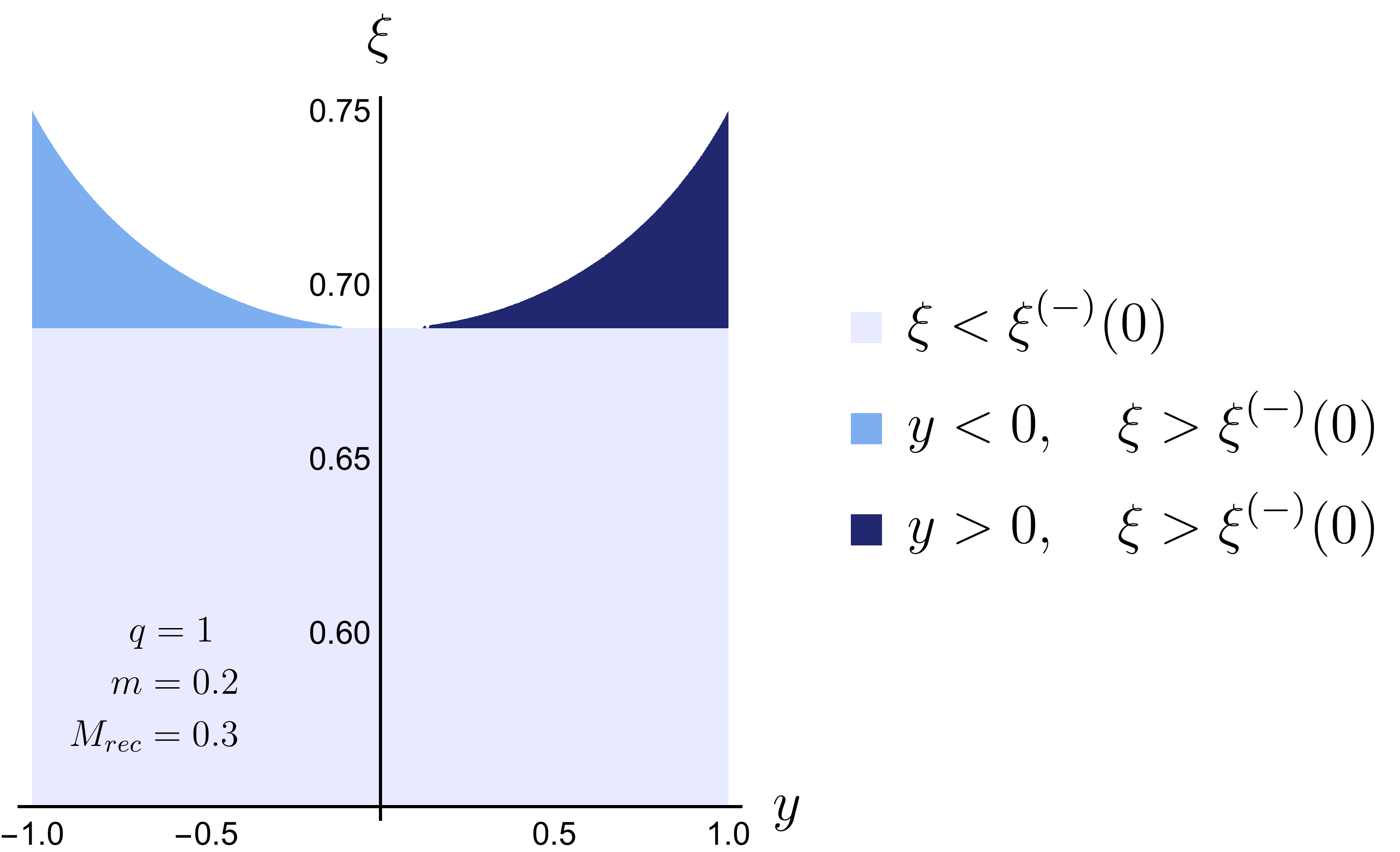
Figure 3: Plot of the physical region in the $\xi y$ plane. The shaded orange region is where $\underline{k}_{n}^{(+)}(\xi,y)$ is negative. It is physically equivalent to the (positive) $\underline{k}_{n}^{(-)}(\xi,-y)$ solution in the dark blue region. If we insisted upon considering only positive $\underline{k}_{n}$ solutions, the blue region would be doubly covered, and the dark blue one would not be there.

we display the $\xi,y$ kinematic region. We remark that the negative $\underline{k}_{n}^{(+)}(\xi,y)$ region includes neither soft nor collinear singularities, since $\xi$ is large, and since the angular separation of the quark and the radiated gluon is larger than $\pi/2$. From now on we will drop the suffix $(-)$ and will use $\xi(y)$ and $\xi(0)$ instead of $\xi^{(-)}(y)$ and $\xi^{(-)}(0)$.

In fig. 4 we show the partition o the kinematic region represented in the more familiar Dalitz plane.

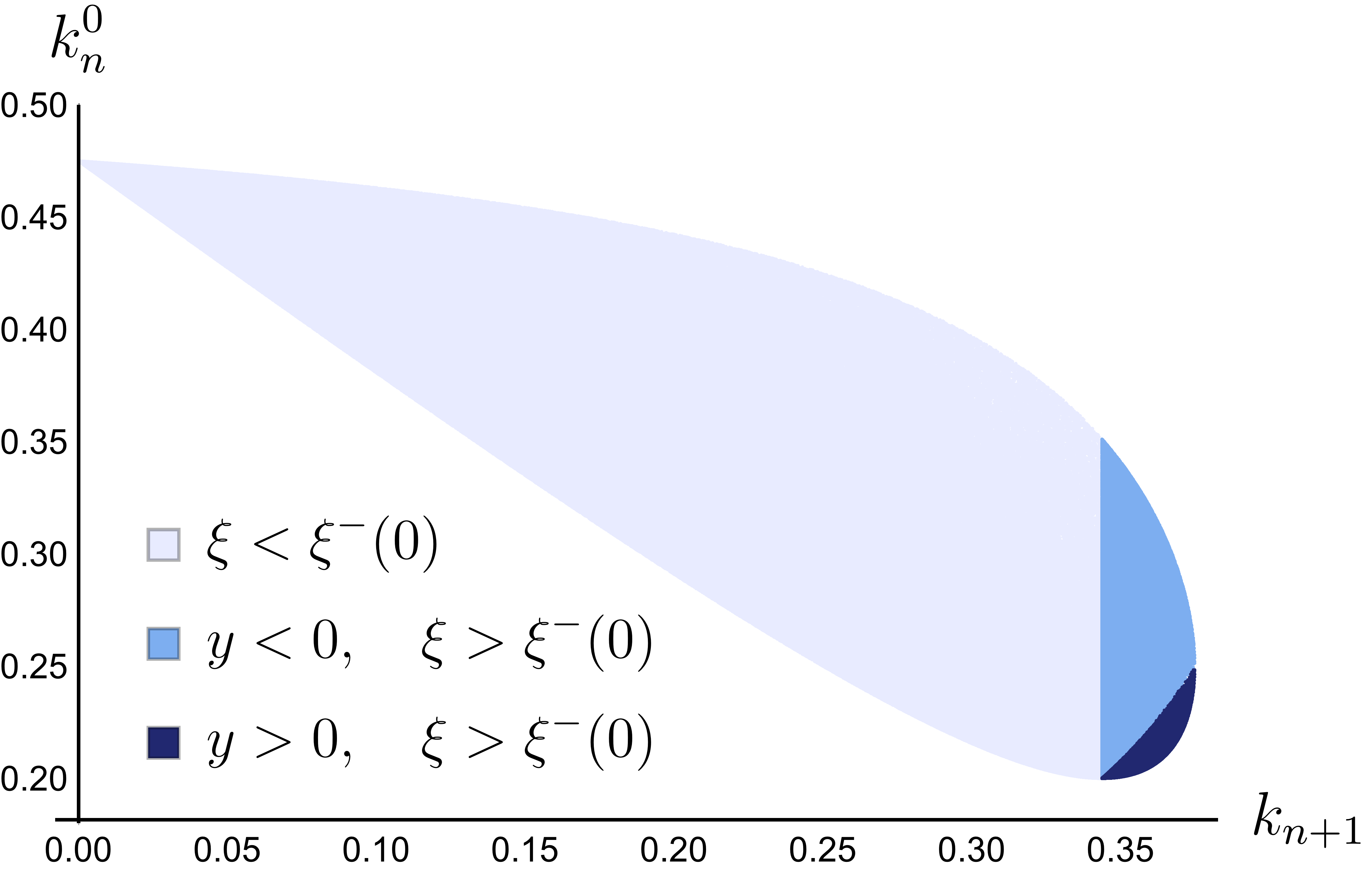
Figure 4: Dalitz plot for the three-body phase space of the system comprising the heavy flavour, the radiated gluon and the recoiling system.

Notice that in the massless limit the physical region in the Dalitz plot develops an acute angle in the lower right, corner corresponding to the gluon being anticollinear with the $b$ quark. Thus, the problematic region $\xi>\xi(0)$ is not a singular one.

2.3 Full kinematic reconstruction of the real emission

So far, we have got the length of the tri-vectors $\vec{k}_{n}$ and $\vec{k}_{n+1}$. It is a standard kinematical problem to determine their directions in such a way that their sum $\vec{k}$ is parallel to $\vec{\overline{k}}_{n}$. We do not enter in further details about it.

The last step is to calculate the $\beta$ parameter of the boost transformation $\Lambda$, eq. (15), and to boost “back” the other barred momenta in the real event

$$k_{i}=\Lambda^{-1}\overline{k}_{i},\quad i=1,\cdots,n-1.$$ (32)

The above mapping allows us to write the $(n+1)$-body phase space element in the factorized form

$$\mathrm{d}\Phi_{n+1}=\mathrm{d}\Phi_{\text{rad}}\mathrm{d}\overline{\Phi}_{n}=J(\xi,y,\phi)\mathrm{d}\xi\mathrm{d}y\mathrm{d}\phi\mathrm{d}\overline{\Phi}_{n},$$ (33)

where we have expressed the radiation phase space in terms of the FKS variables with the jacobian function $J(\xi,y,\phi)$ taking into account the change of variables involved in the transformation. In order to extract the jacobian, we have to manipulate and compare the l.h.s and the r.h.s of eq. (33). Recalling eq. (8), we perform the change of variables

$$\vec{k}_{n}\to\vec{k}-\vec{k}_{n+1}$$ (34)

in the three-body phase space, eq. (9),

$$\begin{split}\mathrm{d}\Phi_{3}&=\frac{\mathrm{d}M^{2}_{\text{rec}}}{2\pi}\frac{\mathrm{d}^{3}\vec{k}}{2k^{0}_{n}(2\pi)^{3}}\frac{\mathrm{d}^{3}\vec{k}_{n+1}}{2k^{0}_{n+1}(2\pi)^{3}}\frac{\mathrm{d}^{3}\vec{k}_{\text{rec}}}{2k^{0}_{\text{rec}}(2\pi)^{3}}\\ &\hskip 14.22636pt\times(2\pi)^{4}\delta^{(4)}(q-k-k_{\text{rec}})\,.\end{split}$$ (35)

In polar coordinates, we have

$$\mathrm{d}^{3}\vec{k}=\underline{k}^{2}\mathrm{d}\underline{k}\mathrm{d}\Omega$$ (36)

and, using as reference direction that of $\vec{k}$,

$$\frac{\mathrm{d}^{3}\vec{k}_{n+1}}{2k^{0}_{n+1}(2\pi)^{3}}=\frac{q^{2}}{(4\pi)^{3}}\xi\mathrm{d}\xi\mathrm{d}\cos{\alpha}\mathrm{d}\phi\,,$$ (37)

where $\alpha$ is the angle between $\vec{k}_{n+1}$ and $\vec{k}$ and $\phi$ is the azimuthal angle taking $\vec{k}$ as the reference direction. Hence

$$\begin{split}\mathrm{d}\Phi_{n+1}&=\frac{q^{2}}{(4\pi)^{3}}\xi\mathrm{d}\xi\mathrm{d}\cos{\alpha}\mathrm{d}\phi\frac{\underline{k}^{2}\mathrm{d}\underline{k}\mathrm{d}\Omega}{2k^{0}_{n}(2\pi)^{3}}\frac{\mathrm{d}M^{2}_{\text{rec}}}{2\pi}\\ &\hskip 14.22636pt\times\frac{\mathrm{d}^{3}k_{\text{rec}}}{2k^{0}_{\text{rec}}(2\pi)^{3}}(2\pi)^{4}\delta^{(4)}(q-k-k_{\text{rec}})\mathrm{d}\Phi_{\text{rec}}.\end{split}$$ (38)

On the other hand, following the same arguments that led to eq. (8), we can split the barred Born phase space into a two-body phase space and the phase space of the system recoiling against the emitting parton

$$\begin{split}\mathrm{d}\overline{\Phi}_{n}&=\frac{\mathrm{d}\overline{M}^{2}_{\text{rec}}}{2\pi}\frac{\mathrm{d}^{3}\overline{\vec{k}}_{n}}{2\overline{k}^{0}_{n}(2\pi)^{3}}\frac{\mathrm{d}^{3}\overline{\vec{k}}_{\text{rec}}}{2\overline{k}^{0}_{\text{rec}}(2\pi)^{3}}\\ &\hskip 14.22636pt\times(2\pi)^{4}\delta^{(4)}(q-\overline{k}_{n}-\overline{k}_{\text{rec}})\mathrm{d}\overline{\Phi}_{rec}.\end{split}$$ (39)

Since $\overline{k}_{n}=q-\Lambda k_{\text{rec}}$, the delta function in eq. (39) constrains the value of $\overline{k}_{\text{rec}}$ to be

$$\overline{k}_{\text{rec}}=\Lambda k_{\text{rec}}.$$ (40)

Then, exploiting the Lorentz invariance of the phase space element, we have

$$\begin{split}&\frac{\mathrm{d}M^{2}_{\text{rec}}}{2\pi}\frac{\mathrm{d}^{3}\vec{k}_{\text{rec}}}{2k^{0}_{\text{rec}}(2\pi)^{3}}(2\pi)^{4}\delta^{(4)}(q-k-k_{\text{rec}})\mathrm{d}\Phi_{\text{rec}}=\\ &\phantom{aaaa}\frac{\mathrm{d}\overline{M}^{2}_{\text{rec}}}{2\pi}\frac{\mathrm{d}^{3}\overline{\vec{k}}_{\text{rec}}}{2\overline{k}^{0}_{\text{rec}}(2\pi)^{3}}(2\pi)^{4}\delta^{(4)}(q-\overline{k}_{n}-\overline{k}_{\text{rec}})\mathrm{d}\overline{\Phi}_{\rm rec},\end{split}$$ (41)

where the r.h.s and the l.h.s are related by the boost transformation $\Lambda$. In particular, we observe that

$$\Lambda(q-k)=\Lambda k_{\text{rec}}=q-\overline{k}_{n},$$ (42)

so that the boost maps the argument of the delta function in the r.h.s into that of the delta function in the l.h.s. Inserting eq.(38) and eq.(39) into eq.(33) and using eq.(41), we get

$$\begin{split}&\frac{q^{2}}{(4\pi)^{3}}\xi\mathrm{d}\xi\,\mathrm{d}\cos{\alpha}\,\mathrm{d}\phi\frac{\underline{k}^{2}\mathrm{d}\underline{k}\mathrm{d}\Omega}{2k^{0}_{n}(2\pi)^{3}}=\\ &\phantom{aaaaaaaaaaaaaaaaaaa}J(\xi,y,\phi)\mathrm{d}\xi\,\mathrm{d}y\,\mathrm{d}\phi\frac{\mathrm{d}^{3}\overline{k}_{n}}{2\overline{k}^{0}_{n}(2\pi)^{3}}.\end{split}$$ (43)

By virtue of the mapping, the vectors $\vec{k}$ and $\vec{\overline{k}}_{n}$ are parallel so that in polar coordinates their angular elements are equal, $d\Omega=d\overline{\Omega}_{n}$. Then, from eq. (43) we have

$$\frac{q^{2}}{(4\pi)^{3}}\xi\frac{\underline{k}^{2}}{k_{n}^{0}}\mathrm{d}\cos{\alpha}\,\mathrm{d}\underline{k}=J(\xi,y,\phi)\frac{\overline{\underline{k}}_{n}^{2}}{\overline{k}_{n}^{0}}\,\mathrm{d}y\,\mathrm{d}\overline{\underline{k}}_{n}.$$ (44)

and we are left with the computation of the jacobian of the two-variable-transformation

$$J^{(2)}=\begin{vmatrix}\dfrac{\partial\overline{\underline{k}}_{n}}{\partial\underline{k}}&\dfrac{\partial y}{\partial\underline{k}}\\[10.00002pt] \dfrac{\partial\overline{\underline{k}}_{n}}{\partial\cos\alpha}&\dfrac{\partial y}{\partial\cos\alpha}\end{vmatrix}.$$ (45)

This transformation is implicitly defined by the relations

$$\begin{split}\underline{k}_{n}&=\sqrt{\underline{k}^{2}+\underline{k}^{2}_{n+1}-2\underline{k}\,\underline{k}_{n+1}\cos\alpha},\quad y=\frac{\underline{k}^{2}-\underline{k}_{n}^{2}-\underline{k}_{n+1}^{2}}{2\underline{k}_{n}\,\underline{k}_{n+1}},\\ M^{2}_{\text{rec}}&=(q^{0}-k_{n}^{0}-\underline{k}_{n+1})^{2}-\underline{k}^{2},\hskip 14.22636pt\overline{\underline{k}}_{n}=\frac{\lambda^{{1}/{2}}(q^{2},M_{\text{rec}}^{2},m^{2})}{2q^{0}},\end{split}$$ (46)

where $\lambda$ is the kinematical Kallen function:

$$\lambda(x,y,z)=x^{2}+y^{2}+z^{2}-2xy-2xz-2yz.$$ (47)

Applying the chain-rule for the derivative, it is straightforward to compute the jacobian. We get

$$J^{(2)}=\frac{1}{\underline{k}_{n}^{3}}\frac{\underline{k}^{2}}{\overline{\underline{k}}_{n}}\frac{\overline{k}_{n}^{0}}{k_{n}^{0}}\big{[}k_{n}^{0}(\overline{k}_{n}^{0}-\underline{k}_{n+1})-m^{2}(1-{\underline{k}_{n+1}}/{q^{0}})\big{]}$$ (48)

The final expression for the full jacobian $J$ is thus

$$\begin{split}J(\xi,y,\phi)&=\frac{q^{2}}{(4\pi)^{3}}\xi\frac{\underline{k}_{n}^{3}}{\overline{\underline{k}}_{n}}\frac{1}{k_{n}^{0}(\overline{k}_{n}^{0}-\underline{k}_{n+1})-m^{2}(1-{\underline{k}_{n+1}}/{q^{0}})}\\ &=\frac{q^{2}}{(4\pi)^{3}}\xi\frac{\underline{k}_{n}^{3}}{\overline{\underline{k}}_{n}}\frac{2}{k_{n}^{0}(2\overline{k}_{n}^{0}-q^{0}\xi)-m^{2}(2-\xi)}\end{split}$$ (49)

Note that the denominator of $J$ vanishes in two regions:

• when approaching the curve $\xi=\xi(0)$ for $y>0$, behaving as $\xi(0)-\xi$

• when approaching the curve $\xi=\xi(y)$, as $\sqrt{\xi(y)-\xi}$.

In the first case, the $k_{n}^{3}$ term in the numerator vanishes simultaneously as $(\xi(0)-\xi)^{3}$. It follows that the jacobian vanishes as $J\sim(\xi(0)-\xi)^{2}$ for $\xi\to\xi(0)$ at fixed $y>0$. This result is coherent with what has been argued above regarding the degenerate points corresponding to the configuration with the emitter parton at rest in the partonic centre-of-mass frame. In the second region, the jacobian develops an integrable singularity, that can be dealt with by importance sampling techniques in Monte Carlo integration.

2.4 Generation of radiation

The POWHEG master formula for the generation of radiation Frixione:2007vw ; Alioli:2010xd is

$$\begin{split}&d\sigma_{\text{NLO}}=\overline{B}(\Phi_{n})d\Phi_{n}\bigg{[}\Delta_{\text{NLO}}(\Phi_{n},t_{\rm min})+\\ &\sum_{\alpha}\frac{\left[d\Phi_{\text{rad}}\Delta_{\text{NLO}}(\Phi_{n},K_{\perp}(\Phi_{n+1}))R(\Phi_{n+1})\right]_{\alpha}^{\overline{\Phi}^{\alpha}_{n}=\Phi_{n}}}{B(\Phi_{n})}\bigg{]},\end{split}$$ (50)

where $t_{\rm min}$ is an infrared cutoff, and the NLO Sudakov form factor is given by

$$\begin{split}&\Delta_{\text{NLO}}(\Phi_{n},p_{T})=\theta(p_{T}-t_{\rm min})\\ &\exp{\left[-\sum_{\alpha}\int\frac{\left[d\Phi_{\text{rad}}R(\Phi_{n+1})\Theta(K_{\perp}(\Phi_{n+1})-p_{T})\right]_{\alpha}^{\overline{\Phi}^{\alpha}_{n}=\Phi_{n}}}{B(\Phi_{n})}\right]}.\end{split}$$ (51)

In the case of a massless emitter, $K_{\perp}$ is a smooth function of the radiation variables, which is required to reduce to the transverse momentum in approaching the soft and collinear limits. For the massive case, in ref. Barze:2012tt the following definition was proposed

$$K_{\perp}^{2}=2\frac{k^{0}}{p^{0}}p\cdot k=\frac{q^{2}}{2}\xi^{2}(1-\beta y_{\text{phy}}).$$ (52)

$y_{\text{phy}}$ denotes the cosine of the physical angle between the emitter and the emitted parton. Eq. (52) has the remarkable property of reducing continuously to the transverse momentum in the massless limit. We assume it as our default scale choice.

According to the standard veto method, we look for a suitable upper bound function $U$ of the integrand in the NLO Sudakov form factor, namely

$$U(\xi,y)d\xi dy\geq\frac{R}{B}J(\xi,y)d\xi dy.$$ (53)

For the sake of simplicity, we have omitted the integration on the azimuthal angle $d\phi$, which results in a constant $2\pi$ factor.
We model the upper bound function on the asymptotic singular behavior of the real matrix element near the soft and collinear singularities. We recall that the jacobian of the mapping has a divergent behaviour near the curve $\xi=\xi(y)$. The upper bound function should have a behaviour not weaker than the Jacobian near the singular regions, and furthermore, it should be simple enough to allow us to perform an analytical integration in the constrained radiation phase space given by the cut $K_{T}^{2}>t$.
It is convenient to perform a change of integration variables from $\xi,\,y$ to $\xi,\,K_{T}^{2}$. Indeed, it turns out that $K_{T}^{2}$ is a monotonic decreasing function of $y$ at fixed $\xi$, i.e. ${\partial K_{T}^{2}}/{\partial y}<0$.
The inversion of this mapping is too complex to be performed analytically, but easy to perform numerically. We find that the associated jacobian ${\partial K_{T}^{2}}/{\partial y}$ has a behaviour similar to that of the jacobian of the mapping $J$:

$$\sim \frac{1}{\sqrt{\xi(y)-\xi}}\;\;\mbox{when}\;\;\xi\rightarrow\xi(y);$$ (54)

$$\sim (\xi(0)-\xi)^{2}\;\;\mbox{when}\;\;\xi\rightarrow\xi(0)\;\;\mbox{for}\;\;y\geq 0.$$ (55)

We now write

$$U=\frac{\partial K_{T}^{2}}{\partial y}U^{\prime},$$ (56)

so that in the new integration variables the integrand becomes $U^{\prime}$

$$\int d\xi\,dy\,\Theta(K_{T}^{2}-t)U=\int d\xi dK_{T}^{2}\Theta(K_{T}^{2}-t)U^{\prime}.$$ (57)

$U^{\prime}$ must have a simple form, and must have the appropriate behaviour to act as an upper bound for the soft and collinear singularities of the real matrix element.

2.4.1 Upper bound function

The singular behaviour of the real matrix element squared is universal and can be extracted in a straightforward manner by means of the eikonal approximation. In terms of the radiation variables, we get

$$\frac{R}{B}\sim\frac{N}{\xi^{2}(1-\beta y_{\text{phy}})}=\frac{N}{K_{T}^{2}},$$ (58)

with $N$ a suitable normalization constant. On the other hand, in the soft limit, the jacobian of the mapping behaves as

$$J(\xi,y)\sim N^{\prime}\xi.$$ (59)

We must also take into account the behaviour in the soft limit of the jacobian term factorized in $U$:

$$\frac{\partial K_{T}^{2}}{\partial y}\sim N^{\prime\prime}\xi^{2}.$$ (60)

Putting all the three contributions together, we obtain the following expression of the upper bound function $U^{\prime}$

$$U^{\prime}(\xi,K_{T}^{2})=\frac{1}{K_{T}^{2}}\times\xi\times\frac{1}{\xi^{2}}=\frac{1}{\xi K_{T}^{2}}.$$ (61)

A more complete analysis shows that mapping $J$ is enhanced (although not divergent) at large $\xi$ for $y\to-1$. In order to get a more efficient upper bound, we add the factor $\frac{1}{1-{K_{T}^{2}}/{q^{2}}}$ to the previous expression. Hence, our final choice for the upper bound function $U^{\prime}$ is

$$U^{\prime}(\xi,K_{T}^{2})=\frac{1}{\xi K_{T}^{2}(1-{K_{T}^{2}}/{q^{2}})}.$$ (62)

2.4.2 Integral of the upper bound function

In order to integrate the upper bound function analytically, its domain of integration has to be suitably enlarged. This can be done by interpreting the $R/B$ expression as being defined in the larger domain, but as vanishing outside of the physical domain. Since the veto procedure prescribes that a point generated according to the upper bound function should be accepted with a probability proportional to the value of the radiation function divided by the upper bound function, points generated outside the physical domain should always be vetoed according to the above interpretation. From eq. (52), we find the upper bound

$$K_{T}^{2}<K_{\text{max}}^{2}\equiv\frac{q^{2}}{2}\xi_{\rm max}^{2}(1+\beta_{0}),$$ (63)

where $\beta_{0}$ is the velocity of the emitter in the underlying Born configuration (this follows from the fact that we always have $\beta\leq\beta_{0}$), and we also find

$$\frac{2K_{T}^{2}}{(1+\beta_{0})}<\xi^{2}<\frac{2K_{T}^{2}}{(1-\beta_{0})},$$ (64)

We thus take as our domain of integration the region in $K_{T}$ and $\xi$ such that eqs. (63) and (64) are satisfied. We notice that in this way $\xi$ can even become larger than 1. In practice, however, adding also the $\xi<1$ or $\xi<\xi_{\rm max}$ limit would render the integration more difficult, so we prefer to deal with it by vetoing. Defining

$$\xi_{\,\stackrel{{\scriptstyle M}}{{m}}{}}(K_{t}^{2})\equiv\sqrt{\frac{2K_{T}^{2}}{q^{2}(1\mp\beta_{0})}},$$ (65)

the integral of the upper bound function is then

$$\begin{split}I(t)&=\int_{t}^{K_{\rm max}^{2}}\frac{dK_{T}^{2}}{K_{T}^{2}(1-{K_{T}^{2}}/{q^{2}})}\int_{\xi_{m}(K_{t}^{2})}^{\xi_{M}(K_{t}^{2})}\frac{d\xi}{\xi}\\ &=\ln\left[\frac{K_{\rm max}^{2}}{q^{2}-K_{\rm max}^{2}}\frac{q^{2}-t}{t}\right]\,y_{0},\end{split}$$ (66)

where $y_{0}\equiv(1/2)\ln[(1+\beta_{0})/(1-\beta_{0})]$ is the rapidity of the emitter in the underlying Born configuration. Given a number $0<r<1$, the $t$ value generated by solving the equation $r=\exp[-2\pi NI(t)]$ is

$$t=\frac{A}{1+A}q^{2},\quad A=\frac{K_{\rm max}^{2}}{q^{2}-K_{\rm max}^{2}}\exp\left[\frac{\log{r}}{2\pi Ny_{0}}\right].$$ (67)

2.4.3 Generation of radiation kinematics

The algorithm for generating the radiation variables proceeds as follows:

1. We set the initial scale $t_{0}=K^{2}_{\rm max}$.

2. We generate a uniform random number

   $$0<r<\exp[-2\pi NI(t_{0})],$$

   and get $t$ from eq. (67). If $t$ is below $t_{\rm min}$, no radiation is generated, and the event is emitted as is.

3. We pick a new uniform random number $0<r^{\prime}<1$ and we generate a value for $\xi$ as

   $$\xi=\xi_{\text{m}}(t)\exp(y_{0}r^{\prime}).$$ (68)

   This is consistent with the distribution of $\xi$ at fixed $K_{T}^{2}$ according to eq. (66).

4. If $\xi>\xi_{\text{max}}$, we set $t_{0}=t$, and go back to the step 2.

5. If the veto condition is passed, given $t$ and $\xi$, we solve numerically for $y$ the implicit equation

   $$K_{T}^{2}(\xi,y)=t.$$ (69)

   If a solution does not exist, we set $t=t_{0}$ and go back to step 2.

6. Now that $\xi$ and $y$ are available, we generate a random $\phi$, and compute the ratio $R=[R/BJ(\xi,y)]/U(\xi,y)]$, with $U$ given in terms of $U^{\prime}$ in eq. (56), and generate a new random number $0<r^{\prime\prime\prime}<1$. If $r^{\prime\prime\prime}>R$ we set $t_{0}=t$ and go back to the step 2. Otherwise, the event is accepted.

3 Phenomenology

3.1 comparison in the bb4l case

We have compared results obtained with the new method presented here, with those obtained with the default POWHEG settings for the bb4l generator of ref. Jezo:2016ujg . We found remarkable agreement between the two results for all the distributions that we have examined. Here we show only two of them, to convey the idea of the quality of the agreement. These results were obtained for the 8TeV LHC collider, using the MSTW2008 PDF Martin:2009iq set for reference only (other sets could be used as well Nadolsky:2008zw ; Ball:2014uwa ). In our simulations we make the $B$ hadrons stable. Jets are reconstructed using the Fastjet Cacciari:2011ma implementation of the anti-$k_{\rm\mathchoice{\displaystyle}{\scriptstyle}{\scriptscriptstyle}{\scriptscriptstyle}T}$ algorithm Cacciari:2008gp with $R=0.5$. We denote as $B$ (${\bar{B}}$) the hardest (i.e. largest $p_{\rm T}$) $b$ ($\bar{b}$) flavoured hadron. The $B$ ($\bar{B}$) jet ${j_{\rm\mathchoice{\displaystyle}{\scriptstyle}{\scriptscriptstyle}{\scriptscriptstyle}B}}$ ($j_{\rm\mathchoice{\displaystyle}{\scriptstyle}{\scriptscriptstyle}{\scriptscriptstyle}{\bar{B}}}$) is defined to be the jet that contains the hardest $B$ ($\bar{B}$). We discard events where the ${j_{\rm\mathchoice{\displaystyle}{\scriptstyle}{\scriptscriptstyle}{\scriptscriptstyle}B}}$ and $j_{\rm\mathchoice{\displaystyle}{\scriptstyle}{\scriptscriptstyle}{\scriptscriptstyle}{\bar{B}}}$ coincide. The hardest $e^{+}$ ($\mu^{-}$) and the hardest $\nu_{e}$ ($\bar{\nu}_{\mu}$) are paired to reconstruct the $W^{+}$ ($W^{-}$). The reconstructed top (antitop) quark is identified with the corresponding $W^{+}j_{B}$ ($W^{-}j_{\bar{B}}$) pair. We show the invariant mass of the $W-b$-jet system (fig. 5)

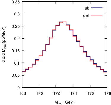
Figure 5: Invariant mass distribution of the reconstructed top quark mass, defined as the mass of the $W^{+}j_{B}$ or $W^{-}j_{\bar{B}}$ system, produced with the bb4l generator, at the 8 TeV LHC. The two distributions are obtained with the default implementation of radiation from $b$ quarks (def), and with the new implementation presented here (alt).

and the $B$ fragmentation function in top decay (Fig. 6),

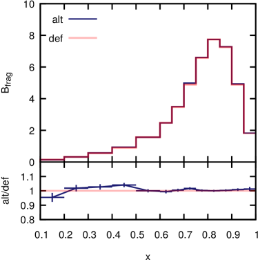
Figure 6: $B$ fragmentation function in top quark decay as defined in ref. Jezo:2016ujg , produced with the bb4l generator for the 8 TeV LHC. The default and alternative implementation of radiation from $b$ quarks are compared.

as defined in ref. Jezo:2016ujg , i.e. the the $B$ energy in the reconstructed top rest frame normalized to the maximum value that it can attain at the given top virtuality. In the curves, the alt (for “alternative”) label stands for our new implementation, while def (for “default”) is the current POWHEG default. As one can see, the agreement is very good. This also shows that details in the implementation of radiation from the $b$ quark in top decays do not seem to have important impact on physical observables.

We found that the efficiency and the generation rate of the new implementation are comparable with those of the POWHEG default.

3.2 $b$ production in hadronic collisions

In this section we study the available POWHEG implementations of radiation from massive quarks for the hvq generator Frixione:2007nw , i.e. the default POWHEG implementation and our new one. In spite of the fact that the default formalism has been available for quite some time Barze:2012tt , no such study has been performed so far. We thus discuss it in this work, where we can also compare with our new implementation.

The hvq generator has been available for quite some time as a tool to generate top, bottom and charm pairs in hadronic collisions. It is designed to simulate correctly the production of a heavy flavour pair when the logarithm of the ratio of the transverse momentum of the heavy quark divided by its mass is not too large. This limitation arises because there are three mechanisms, depicted in figure 7,

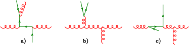
Figure 7: Example diagrams for the three mechanism that give rise to log-enhanced contributions in heavy flavour production: a) final state radiation from a quark; b) gluon splitting; c) flavour excitation.

involving radiation from the final state quark, production of a heavy quark-antiquark pair via final state gluon splitting and the splitting of an initial state gluon into a heavy quark-antiquark pair (where one of the two quarks is scattered at large transverse momentum), that can generate large logarithms involving the mass of the heavy quark. In the inclusive cross section for the production of a heavy quark with a given $p_{T}$, for example, they generate logarithms of $p_{T}/m$ (see ref. Nason:1989zy , eq. (5.1)). The last two mechanisms are commonly referred to as gluon splitting and flavour excitation. In spite of this, the hvq generator has also been used to model relatively large transverse momentum production of heavy flavours, as in ref. Cacciari:2012ny . There, the transverse momentum distribution of the heavy flavoured hadron in hvq was compared with the more accurate (but less exclusive) FONLL prediction Cacciari:1998it . It was found to be in rather good agreement. However, the large uncertainties related to the non-perturbative fragmentation of the heavy quark leads to the suspect that such agreement is at least in part accidental.

We will now compare the results obtained with the default hvq generator, that we will label nol (for “no light”, meaning that the heavy quark is treated as very heavy), that treats as singular regions only the radiation from massless partons (i.e. initial state radiation); hvq with the inclusion of the radiation from the heavy quark as a singular region will be labeled asl (for “as light”, meaning that the heavy quark is treated as a light parton). Furthermore, the default treatment of the heavy quark radiation region will be denoted as def, while the new implementation presented here will be called alt. In figs. 8, 9 and 10

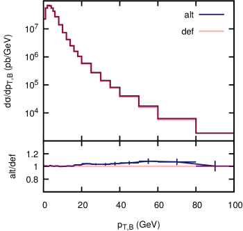
Figure 8: Comparison of alt and def for the transverse momentum distribution of the $B$ hadron at the 8TeV LHC.

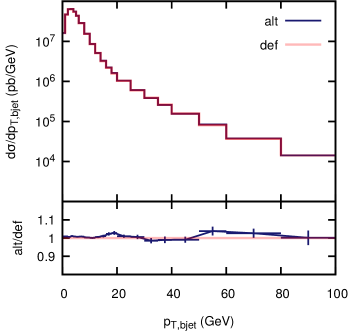
Figure 9: Comparison of alt and def for the transverse momentum distribution of the $b$-jet at the 8TeV LHC.

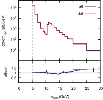
Figure 10: Comparison of alt and def for the $b$-jet mass.

we show a comparison of def and alt. We can immediately see that we do not find important differences between the two methods, consistently with what was found in the bb4l case. The settings are similar to the bb4l case: we make the $B$ hadrons stable, and define the $b$ (${\bar{b}}$) jets as the jets containing the hardest $b$ (${\bar{b}}$) flavoured hadron, with the jets defined as in the bb4l case. However, we do not exclude the case when both hardest $b$-flavoured hadrons are in the same jet. We perform the calculation for the LHC at 8 TeV, using NNPDF30_nlo_as_0118 pdf set Ball:2014uwa . As one can see, the two implementations are in excellent agreement. Observe the jump at 10 GeV in the ${j_{\rm\mathchoice{\displaystyle}{\scriptstyle}{\scriptscriptstyle}{\scriptscriptstyle}B}}$ mass. It is due to the case in which the $b$ and ${\bar{b}}$ flavoured hadrons are both in the jet cone. From figure 10 we also see that for jet masses above 10 GeV the gluon splitting configuration dominates.

We found that the new implementation has a generation efficiency, which is estimated from the numbers of vetoes in FSR generation, three times greater than the default one. This leads to a generation rate of 1316 events per minute, against the 298 events per minute of the POWHEG default, which corresponds to a gain more than a factor of 4.

We now show in the left panels of Figs. 11, 12 and 13

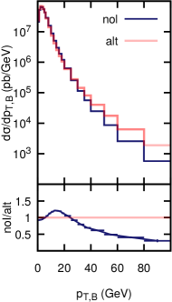
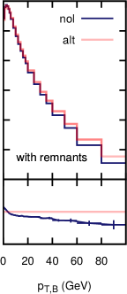
Figure 11: Left panel: comparison of alt and nol for the transverse momentum distribution of the $B$ hadron 8TeV LHC. Right panel: same comparison with the treatment of the enhanced regions using remnants, as discussed in the text.

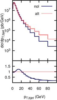
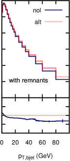
Figure 12: Same as in fig. 11 for the $p_{T}$ of the $b$-jet.

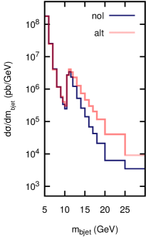
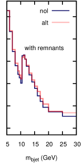
Figure 13: Same as in fig. 11 for the $b$-jet mass.

the comparison among the alt and nol. Here we see considerable differences, especially in the large-momentum tail of the $B$ and ${j_{\rm\mathchoice{\displaystyle}{\scriptstyle}{\scriptscriptstyle}{\scriptscriptstyle}B}}$ transverse momentum distribution, the alt ones being much harder. The mass of the $b$ jet is also remarkably different. The large difference above 10 GeV hints to the fact that heavy quark pair production via the splitting of a large transverse momentum gluon is treated in a very different way in the two cases, and that this difference may be the cause of the large discrepancy in the transverse momentum distribution of the $b$ hadron.

The difference between the alt and nol cases should not come as a surprise. The generation of radiation is performed in the nol case according to the formula

$$\mathrm{d}\sigma = \mathrm{d}\Phi_{B}\tilde{B}(\Phi_{B})\exp\left[\int\frac{R(\Phi_{B},\Phi^{\prime}_{\rm rad})}{B(\Phi_{B})}\theta(k_{t}^{\prime}-k_{t})\mathrm{d}\Phi^{\prime}_{\rm rad}\right]$$ (70)

$$\times \frac{R(\Phi_{B},\Phi_{\rm rad})}{B(\Phi_{B})}\mathrm{d}\Phi_{\rm rad}\,,$$

where $k_{t}$ is the transverse momentum of the emitted gluon with respect to the beam axis, since the only singular regions that are considered there are the initial-state radiation (ISR) ones. The strong coupling constant and the parton densities are evaluated by default at a scale equal to the transverse mass of the heavy quark at the level of the underlying Born kinematics

$$\mu_{f}=\mu_{r}=\sqrt{k_{t,q}^{2}+m_{q}^{2}}$$ (71)

in the $\tilde{B}$ function, while they are evaluated at a scale $k_{t}$ (or $k^{\prime}_{t}$) in the $R/B$ ratios appearing in formula (71). Since $\tilde{B}$ and $B$ are of order $\alpha_{\mathchoice{\displaystyle}{\scriptstyle}{\scriptscriptstyle}{\scriptscriptstyle}\rm S}^{2}$, while $R$ is of order $\alpha_{\mathchoice{\displaystyle}{\scriptstyle}{\scriptscriptstyle}{\scriptscriptstyle}\rm S}^{3}$, this means that in practice two powers of the strong coupling are evaluated at the scale of eq. (71), while one power is evaluated at a scale $k_{t}$. The mismatch in the scale used in $\tilde{B}$ and in the $B$ appearing in the ratios, combined with the exponential, leads as usual to the correct Sudakov form factor for initial state emission.

3.2.1 Problematic regions

In case the transverse momentum of the gluon is small, the scale assignments and the Sudakov form factor describe the process appropriately. It can happen however, that the real emission kinematics is near the gluon splitting, flavour excitation or quark radiation regimes. In these cases the gluon transverse momentum is not small. Furthermore, the numerator $R$ in the integrand may be enhanced with respect to the denominator, thus yielding a damping of the real cross section that is not justified. Also the scale choices are not appropriate. For example, in the case of production of a high transverse momentum heavy quark pair according to the gluon splitting mechanism, the appropriate scale should correspond to two powers of $\alpha_{\mathchoice{\displaystyle}{\scriptstyle}{\scriptscriptstyle}{\scriptscriptstyle}\rm S}$ evaluated at the gluon transverse momentum, and one power of $\alpha_{\mathchoice{\displaystyle}{\scriptstyle}{\scriptscriptstyle}{\scriptscriptstyle}\rm S}$ evaluated at the scale of the order of the invariant mass of the heavy quark pair.

The adoption of the methods illustrated in ref. Barze:2012tt and in the present work for dealing with radiation from a heavy quark leads to the correct treatment of the radiation from the heavy, quark provided all remaining regions are treated correctly. This is in fact what happens in the case of the bb4l generator, where there is only one enhanced region, but it is not the case for the asl generator, that does not treat in a proper way the two regions of gluon splitting and flavour excitation. Thus, the nol and the asl generators will end up treating the enhanced regions in different (and in both cases incorrect) ways. In fact, while in the nol case the enhanced regions will all be treated as if they were ISR processes, in the asl case they will be split, and treated in part as ISR processes, and in part as radiation from the heavy quarks. In order to test this hypothesis, and in order to explore possible strategies to deal with this problem, we proceed as follows. It is possible in POWHEG to further separate out the real cross section into two terms, such that only one term has singular behaviour, while the remaining term, being finite, can be integrated independently. In the hvq case, this means

$$R=R^{(s)}+R^{(r)}\,.$$ (72)

Eq. (70) is then replaced by

$$\mathrm{d}\sigma=\mathrm{d}\Phi_{B}\tilde{B}^{(s)}(\Phi_{B})\exp\left[\int\frac{R^{(s)}(\Phi_{B},\Phi^{\prime}_{\rm rad})}{B(\Phi_{B})}\theta(k_{t}^{\prime}-k_{t})\mathrm{d}\Phi^{\prime}_{\rm rad}\right]$$

$$\times\frac{R^{(s)}(\Phi_{B},\Phi_{\rm rad})}{B(\Phi_{B})}\mathrm{d}\Phi_{\rm rad}+\int\mathrm{d}\Phi_{B}\mathrm{d}\Phi_{\rm rad}R^{(r)}(\Phi_{B},\Phi_{\rm rad})\,.$$ (73)

We can exploit this mechanism in order to separate out the enhanced regions, in such a way that we can treat them in a more uniform way with our generators. In particular, we separate out the gluon splitting and flavour excitation processes in all cases. In the nol case we also separate out the regions of radiation from the heavy quarks, in such a way that they are treated in a more transparent way. Observe that in performing this separation we rely upon the fact that the three enhanced region are not really singular, since the quark mass cuts off the collinear singularities, and thus the remnant term is actually finite.

We define the distance of a real configuration from a given enhanced region as follows

$$\begin{array}[]{lll}d_{\rm isr}&=k_{t}^{2},\phantom{aaaaaaaaaaaaaa}d_{\rm glsp}&=2k_{q}\cdot k_{\bar{q}}\frac{k_{q}^{0}k_{\bar{q}}^{0}}{(k_{q}^{0}+k_{\bar{q}}^{0})^{2}},\\ d_{q}&=2k_{q}\cdot k\frac{k^{0}}{k_{q}^{0}}+m_{q}^{2},\hfill\hfill d_{\bar{q}}&=2k_{\bar{q}}\cdot k\frac{k^{0}}{k_{\bar{q}}^{0}}+m_{q}^{2},\\ d_{q,{\rm flex}}&=k_{{\bar{q}},\perp}^{2}+m_{q}^{2},\hfill\hfill d_{{\bar{q}},{\rm flex}}&=k_{q,\perp}^{2}+m_{q}^{2},\end{array}$$ (74)

where in the first line the distances for ISR and gluon splitting are given, in the second line those for radiation from the heavy quarks, and in the last line the ones for flavour excitation. We then define, for the nol generator

$$D = \frac{d_{\rm isr}^{-1}}{d_{\rm isr}^{-1}+d_{\rm glsp}^{-1}+d_{q}^{-1}+d_{\bar{q}}^{-1}+d_{q,{\rm flex}}^{-1}+d_{{\bar{q}},{\rm flex}}^{-1}},$$

$$R^{(s)} = RD,\qquad R^{(r)}=R(1-D)\,.$$ (75)

For the alt and def generators, we define

$$D = \frac{d_{\rm isr}^{-1}+d_{q}^{-1}+d_{\bar{q}}^{-1}}{d_{\rm isr}^{-1}+d_{\rm glsp}^{-1}+d_{q}^{-1}+d_{\bar{q}}^{-1}+d_{q,{\rm flex}}^{-1}+d_{{\bar{q}},{\rm flex}}^{-1}}$$ (76)

$$R_{i}^{(s)} = R_{i}D,\qquad R_{i}^{(r)}=R_{i}(1-D)\,,$$ (77)

where the index $i$ labels the three singular regions that POWHEG is handling. In this case, the cross section is damped if the kinematics is near a singular region that is nether ISR nor FSR, i.e. only gluon splitting and flavour excitation kinematics are separated into the $(r)$ component.

There is one more issue that needs to be considered when using a damping factor in POWHEG. By default, when evaluating the $R^{(r)}$ component (called “real remnant”), the scale choice is the same as for $\tilde{B}$, i.e. it is eq. (71) applied to the underlying Born kinematics, that depends upon the considered singular region. This would lead to a different scale choice for the remnants in nol and asl. In order to avoid that, we should set the scale on the basis of the real kinematics. This can be done in POWHEG by setting appropriate flags and by modifying the code that computes the scales for the process. Our scale choice is

$$\mu_{f}=\mu_{r}=\frac{1}{2}\left[\sqrt{k_{t,q}^{2}+m_{q}^{2}}+\sqrt{k_{t,{\bar{q}}}^{2}+m_{q}^{2}}+k_{t}\right]\,,$$ (78)

that has the correct limit to the underlying Born scale both in the ISR and in the FSR case.

The result of this procedure is shown in the right panels of Figs. 11, 12 and 13. We notice a remarkable improvement in the agreement, although some important differences do remain. This is not unexpected, since in the two cases radiation from the heavy quark is treated in a very different way. It is interesting to notice that the $B$ and the ${j_{\rm\mathchoice{\displaystyle}{\scriptstyle}{\scriptscriptstyle}{\scriptscriptstyle}B}}$ spectra computed with the nol without remnants (which is the default in the standard hvq generator), is in fair agreement with the alt one when the enhanced regions are separated using the remnants. Since the default hvq program gives a description of the transverse momentum distribution of $B$ hadrons that is in fair agreement with the FONLL calculation, we infer that also the alt prediction will display a similar agreement, provided the gluon splitting and flavour excitation region are treated separately as remnants.

The alt (or equivalently the def generator), with the remnant separation discussed above, seems to be at this point the generator that may give the best description of $b$ production data at hadron collider. We should not forget, however, that some flexibility still remains in the treatment of the remnant (in this work we have made a definite scale choice for the remnants in order to have a clearer comparison with the nol generator). We also notice from figs. 11 and 12 that after the remnants are introduced, the $B$-hadron and $b$-jet $p_{T}$ spectra become softer. This seems to be in contrast with the discussion at the beginning of sec. 3.2.1. On the other hand, this result may be due to the particular scale choice that we have performed for the real graphs, and that POWHEG applies automatically also to the remnants. This scale turns out to be higher than the typical scale involved in the region discussed at the beginning of sec. 3.2.1. A better approach would be to introduce the possibility of alternative scale choices in the remnants, including the possibility of performing a different scale choice depending upon which enhanced region one is considering. We refrain here from carrying out such study, since we believe that comparison with data on single inclusive $b$-hadron and $b$-jet production (see ref. Khachatryan:2011mk ; Aad:2012jga ; Acosta:2004yw and references therein) and on correlations of $b\bar{b}$ pairs Abbott:1999se ; Khachatryan:2011wq , would be needed in order to make progress in this direction, and this is beyond the scope of the present work. Such study would however be very valuable, and not only for the purpose of testing QCD in bottom production. The production of top pairs is one of the most important background process at the LHC, including also its future high luminosity and eventually high energy developments. An accurate simulation of the $t\bar{t}$ background would be very valuable for the LHC experimental collaborations, and it is quite clear that a model of $b$ production yielding a good description of the data from low to high transverse momenta should be also well suited to describe top production in all the needed phase space. Furthermore, these studies could lead to an improved description of top production at large transverse momentum, that, as reported currently by CMS and ATLAS (see Sirunyan:2017mzl ; Aaboud:2016iot and references therein) seems to be not well described by theoretical models.

4 Conclusions

In this paper we have presented a method for implementing radiation from a heavy quark in the POWHEG framework. This method is considerably simpler and more transparent than the one presented in ref. Barze:2012tt , and it has a much better numerical performance. The present method overcomes a problem related to the fact that the most natural map from an underlying Born configuration and a set of FKS-like radiation variables for radiation from a massive quark does not have a unique inverse in the whole kinematic region. The POWHEG inverse map has thus two solutions in some region of phase space, and in the present work it is shown how, by giving up the physical connection of the $y$ variable to the gluon emission angle in a very limited region of phase space one can pick one of the two solutions in such a way that we still have a single valued inverse mapping. We have examined the output of the new method in the framework of the generators of ref. Jezo:2016ujg and Frixione:2007nw . We found that the new method yields results that are very consistent with the previous one, that is at this moment the POWHEG default. This is reassuring, since it shows that details of the implementation do not impact in a visible way the physics result, and also it shows that the previous implementation, in spite of being quite contrived, is in fact correct.

In this work we have also examined for the first time the impact of the inclusion of the singular region associated with radiation from the heavy quark in the case of the hvq generator. We have shown that, unless one separates the enhanced gluon splitting and flavour excitation contribution from the real contribution that are dealt with by the POWHEG radiation formula, and treats them as remnants, one finds results that are in considerable disagreement with the traditional hvq implementation. On the other hand, it seems that performing this separation is the appropriate thing to do for a consistent modeling of the process. We notice that such modeling would be of great interest also for its potential application to top pair production, that is a very important background to many LHC physics studies.

- (1) ATLAS Collaboration, M. Aaboud et al., Evidence for the decay with the ATLAS detector, arXiv:1708.03299.
- (2) CMS Collaboration, C. Collaboration, Evidence for the decay of the Higgs Boson to Bottom Quarks, .
- (3) CMS Collaboration, C. Collaboration, Inclusive search for the standard model Higgs boson produced in pp collisions at using H decays, .
- (4) M. Cacciari, M. Greco, and P. Nason, The P(T) spectrum in heavy flavor hadroproduction, JHEP 05 (1998) 007, [hep-ph/9803400].
- (5) M. Cacciari, S. Frixione, N. Houdeau, M. L. Mangano, P. Nason, and G. Ridolfi, Theoretical predictions for charm and bottom production at the LHC, JHEP 10 (2012) 137, [arXiv:1205.6344].
- (6) T. Sjöstrand, S. Ask, J. R. Christiansen, R. Corke, N. Desai, P. Ilten, S. Mrenna, S. Prestel, C. O. Rasmussen, and P. Z. Skands, An Introduction to PYTHIA 8.2, Comput. Phys. Commun. 191 (2015) 159–177, [arXiv:1410.3012].
- (7) J. Bellm et al., Herwig 7.1 Release Note, arXiv:1705.06919.
- (8) S. Schumann and F. Krauss, A Parton shower algorithm based on Catani-Seymour dipole factorisation, JHEP 03 (2008) 038, [arXiv:0709.1027].
- (9) S. Catani, S. Dittmaier, M. H. Seymour, and Z. Trocsanyi, The Dipole formalism for next-to-leading order QCD calculations with massive partons, Nucl. Phys. B627 (2002) 189–265, [hep-ph/0201036].
- (10) S. Höche and S. Prestel, The midpoint between dipole and parton showers, Eur. Phys. J. C75 (2015), no. 9 461, [arXiv:1506.05057].
- (11) A. Gehrmann-De Ridder, M. Ritzmann, and P. Z. Skands, Timelike Dipole-Antenna Showers with Massive Fermions, Phys. Rev. D85 (2012) 014013, [arXiv:1108.6172].
- (12) A. Gehrmann-De Ridder and M. Ritzmann, NLO Antenna Subtraction with Massive Fermions, JHEP 07 (2009) 041, [arXiv:0904.3297].
- (13) S. Frixione, P. Nason, and B. R. Webber, Matching NLO QCD and parton showers in heavy flavor production, JHEP 08 (2003) 007, [hep-ph/0305252].
- (14) S. Frixione, P. Nason, and G. Ridolfi, A Positive-weight next-to-leading-order Monte Carlo for heavy flavour hadroproduction, JHEP 09 (2007) 126, [arXiv:0707.3088].
- (15) L. Barze, G. Montagna, P. Nason, O. Nicrosini, and F. Piccinini, Implementation of electroweak corrections in the POWHEG BOX: single W production, JHEP 04 (2012) 037, [arXiv:1202.0465].
- (16) J. M. Campbell, R. K. Ellis, P. Nason, and E. Re, Top-pair production and decay at NLO matched with parton showers, JHEP 04 (2015) 114, [arXiv:1412.1828].
- (17) T. Ježo, J. M. Lindert, P. Nason, C. Oleari, and S. Pozzorini, An NLO+PS generator for and production and decay including non-resonant and interference effects, Eur. Phys. J. C76 (2016), no. 12 691, [arXiv:1607.04538].
- (18) S. Frixione, Z. Kunszt, and A. Signer, Three jet cross-sections to next-to-leading order, Nucl. Phys. B467 (1996) 399–442, [hep-ph/9512328].
- (19) S. Frixione, P. Nason, and C. Oleari, Matching NLO QCD computations with Parton Shower simulations: the POWHEG method, JHEP 11 (2007) 070, [arXiv:0709.2092].
- (20) S. Alioli, P. Nason, C. Oleari, and E. Re, A general framework for implementing NLO calculations in shower Monte Carlo programs: the POWHEG BOX, JHEP 06 (2010) 043, [arXiv:1002.2581].
- (21) A. D. Martin, W. J. Stirling, R. S. Thorne, and G. Watt, Parton distributions for the LHC, Eur. Phys. J. C63 (2009) 189–285, [arXiv:0901.0002].
- (22) P. M. Nadolsky, H.-L. Lai, Q.-H. Cao, J. Huston, J. Pumplin, D. Stump, W.-K. Tung, and C. P. Yuan, Implications of CTEQ global analysis for collider observables, Phys. Rev. D78 (2008) 013004, [arXiv:0802.0007].
- (23) NNPDF Collaboration, R. D. Ball et al., Parton distributions for the LHC Run II, JHEP 04 (2015) 040, [arXiv:1410.8849].
- (24) M. Cacciari, G. P. Salam, and G. Soyez, FastJet User Manual, Eur. Phys. J. C72 (2012) 1896, [arXiv:1111.6097].
- (25) M. Cacciari, G. P. Salam, and G. Soyez, The Anti-k(t) jet clustering algorithm, JHEP 04 (2008) 063, [arXiv:0802.1189].
- (26) P. Nason, S. Dawson, and R. K. Ellis, The One Particle Inclusive Differential Cross-Section for Heavy Quark Production in Hadronic Collisions, Nucl. Phys. B327 (1989) 49–92. [Erratum: Nucl. Phys.B335,260(1990)].
- (27) CMS Collaboration, V. Khachatryan et al., Measurement of the Production Cross Section in pp Collisions at TeV, Phys. Rev. Lett. 106 (2011) 112001, [arXiv:1101.0131].
- (28) ATLAS Collaboration, G. Aad et al., Measurement of the b-hadron production cross section using decays to final states in pp collisions at sqrt(s) = 7 TeV with the ATLAS detector, Nucl. Phys. B864 (2012) 341–381, [arXiv:1206.3122].
- (29) CDF Collaboration, D. Acosta et al., Measurement of the meson and hadron production cross sections in collisions at GeV, Phys. Rev. D71 (2005) 032001, [hep-ex/0412071].
- (30) D0 Collaboration, B. Abbott et al., The production cross section and angular correlations in collisions at TeV, Phys. Lett. B487 (2000) 264–272, [hep-ex/9905024].
- (31) CMS Collaboration, V. Khachatryan et al., Measurement of Angular Correlations based on Secondary Vertex Reconstruction at TeV, JHEP 03 (2011) 136, [arXiv:1102.3194].
- (32) CMS Collaboration, A. M. Sirunyan et al., Measurement of normalized differential t-tbar cross sections in the dilepton channel from pp collisions at sqrt(s) = 13 TeV, arXiv:1708.07638.
- (33) ATLAS Collaboration, M. Aaboud et al., Measurement of top quark pair differential cross-sections in the dilepton channel in collisions at = 7 and 8 TeV with ATLAS, Phys. Rev. D94 (2016), no. 9 092003, [arXiv:1607.07281].