Spectral analysis of jet turbulence

Abstract

Informed by LES data and resolvent analysis of the mean flow, we examine the structure of turbulence in jets in the subsonic, transonic, and supersonic regimes. Spectral (frequency-space) proper orthogonal decomposition is used to extract energy spectra and decompose the flow into energy-ranked coherent structures. The educed structures are generally well predicted by the resolvent analysis. Over a range of low frequencies and the first few azimuthal mode numbers, these jets exhibit a low-rank response characterized by Kelvin-Helmholtz (KH) type wavepackets associated with the annular shear layer up to the end of the potential core and that are excited by forcing in the very-near-nozzle shear layer. These modes too the have been experimentally observed before and predicted by quasi-parallel stability theory and other approximations–they comprise a considerable portion of the total turbulent energy. At still lower frequencies, particularly for the axisymmetric mode, and again at high frequencies for all azimuthal wavenumbers, the response is not low rank, but consists of a family of similarly amplified modes. These modes, which are primarily active downstream of the potential core, are associated with the Orr mechanism. They occur also as sub-dominant modes in the range of frequencies dominated by the KH response. Our global analysis helps tie together previous observations based on local spatial stability theory, and explains why quasi-parallel predictions were successful at some frequencies and azimuthal wavenumbers, but failed at others.

1 Introduction

Large-scale coherent structures in the form of wavepackets play an important role in the dynamics and acoustics of turbulent jets. In particular, their spatial coherence makes wavepackets efficient sources of sound (Crighton & Huerre, 1990; Jordan & Colonius, 2013). They are most easily observed in forced experiments, where periodic exertion establishes a phase-reference. The measurements of a periodically forced turbulent jet by Crow & Champagne (1971) served as a reference case for wavepacket models. Early examples of such models include the studies by Michalke (1971) and Crighton & Gaster (1976), who established the idea that the coherent structures can be interpreted as linear instability waves evolving around the turbulent mean flow.

Wavepackets in unforced jets exhibit intermittent behavior (Cavalieri et al., 2011) and as a result are best understood as statistical objects that emerge from the stochastic turbulent flow. We use spectral proper orthogonal decomposition (Lumley, 1970; Towne et al., 2017c) to extract these structures from the turbulent flow. SPOD has been applied to a range of jets using data from both experimental (Glauser et al., 1987; Arndt et al., 1997; Citriniti & George, 2000; Suzuki & Colonius, 2006; Gudmundsson & Colonius, 2011), and numerical studies (Sinha et al., 2014; Towne et al., 2015; Schmidt et al., 2017).

Wavepackets have been extensively studied, mainly because of their prominent role in the production of jet noise, and models based on the parabolized stability equations (PSE) have proven to be successful at modeling them (Gudmundsson & Colonius, 2011; Cavalieri et al., 2013; Sinha et al., 2014). This agreement between SPOD modes and PSE solution breaks down at low frequencies and for some azimuthal wavenumbers, and in general downstream of the potential core. In the present study, we show that the SPOD eigenspectra unveil low-rank dynamics, and we inspect the corresponding modes and compare them with predictions based on resolvent analysis. The results show that two different mechanisms are active in turbulent jets, and they explain the success and failure of linear and PSE models.

Resolvent analysis of the turbulent mean flow field seeks sets of forcing and response modes that are optimal with respect to the energetic gain between them. When applied to the mean of a fully turbulent flow, the resolvent forcing modes can be associated with nonlinear modal interactions (McKeon & Sharma, 2010) as well as stochastic inputs to the flow, for example the turbulent boundary layer in the nozzle that feeds the jet. Garnaud et al. (2013) interpreted the results of their resolvent analysis of a turbulent jet in the light of experimental studies of forced jets by Moore (1977) and Crow & Champagne (1971). They found that the frequency of the largest gain approximately corresponds to what the experimentalists referred to as the preferred frequency, i.e. the frequency where external harmonic forcing in the experiments triggered the largest response. In the context of jet aeroacoustics, Jeun et al. (2016) restricted the optimal forcing to vortical perturbations close to the jet axis, and the optimal responses to the far-field pressure. Their results show that suboptimal modes have to be considered in resolvent-based jet noise models.

In this paper, we use resolvent analysis to model and explain the low-rank behavior of turbulent jets revealed by SPOD. Recent theoretical connections between SPOD and resolvent analysis (Towne et al., 2015; Semeraro et al., 2016; Towne et al., 2017c) make the latter a natural tool for this endeavor and provide a framework for interpreting our results.

The remainder of the paper is organized as follows. The three large-eddy simulation databases used to study different Mach number regimes are introduced in §2. At first, the focus is on the lowest Mach number case in §§3-5. We start by analyzing the data of this case using (mainly) SPOD in §3, followed by the resolvent analysis in §4. The results of the SPOD and the resolvent model are compared in §5. §6 addresses Mach number effects observed in the remaining two cases representing the transonic and the supersonic regime. Finally, the results are discussed in §7. For completeness, we report in appendix A all results for the higher Mach number cases that were omitted in §6 for brevity.

2 Large eddy simulation

The unstructured flow solver “Charles” (Brès et al., 2017b) is used to perform large-eddy simulations of three turbulent jets at Mach numbers $M_{j}=U_{j}/a_{j}$ of 0.4, 0.9, and 1.5. All jets are isothermal and the supersonic jet is ideally expanded. The nozzle geometry is included in the computational domain, and synthetic turbulence combined with a wall model is applied inside the nozzle to obtain a fully turbulent boundary layer inside the nozzle. The jets are further characterized by their Reynolds numbers $\Rey=\rho_{j}U_{j}D/\mu_{j}$, which correspond approximately to the laboratory values in a set of companion experiments. The reader is referred to Brès et al. (2017b) for further details on the numerical method, meshing strategy and subgrid-scale model. A detailed validation of the $M_{j}=0.9$ jet including the nozzle-interior turbulence modeling (i.e., synthetic turbulence, wall model) can be found in Brès et al. (2017a). The subscripts $j$ and $\infty$ refer to jet and free-stream conditions, $a$ is the speed of sound, $\rho$ density, $D$ nozzle diameter, $\mu$ dynamic viscosity, $T$ temperature, and $U_{j}$ to the axial jet velocity on the centerline of the nozzle exit, respectively. Throughout this paper, the flow is non-dimensionalized by its nozzle exit values, pressure by $\rho_{j}U_{j}^{2}$, lengths by $D$, and time by $D/U_{j}$. Frequencies are reported in terms of the Strouhal number $\mbox{{St}}=\omega/(2\pi M_{j})$, where $\omega$ is the non-dimensional angular frequency.

case	$M_{j}$	$\Rey$	$\frac{p_{0}}{p_{\infty}}$	$\frac{T_{0}}{T_{\infty}}$	$n_{\text{cells}}$	$\frac{\differential tc_{\infty}}{D}$	$\frac{t_{\text{sim}}c_{\infty}}{D}$
subsonic	0.4	$0.45\cdot 10^{6}$	1.117	1.03	$15.9\cdot 10^{6}$	$1\cdot 10^{-3}$	2000
transsonic	0.9	$1.01\cdot 10^{6}$	1.7	1.15	$15.9\cdot 10^{6}$	$1\cdot 10^{-3}$	2000
supersonic	1.5	$1.76\cdot 10^{6}$	3.67	1.45	$31\cdot 10^{6}$	$2.5\cdot 10^{-4}$	500

Table 1: Parameters of the large-eddy simulations.

The parameters of the three simulations are listed in table 1: ${p_{0}}/{p_{\infty}}$ is the nozzle pressure ratio, ${T_{0}}/{T_{\infty}}$ the nozzle temperature ratio, $n_{\text{cells}}$ the number of control volumes, ${\differential tc_{\infty}}/{D}$ the computational time step, and ${t_{\text{sim}}/c_{\infty}}{D}$ the total simulation time after the flow became stationary, i.e. without initial transients.

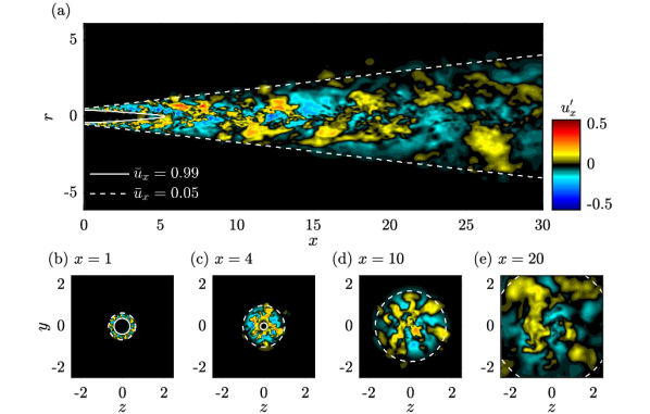
Figure 1: Instantaneous flow field of the subsonic jet: (a) streamwise cross-section along the jet axis; (b-e) transverse planes at different streamwise locations $x$. The streamwise velocity fluctuation ${u}^{\prime}_{x}$ is shown. The potential core and the jet width are indicated as lines of constant $\bar{u}_{x}$ at 99% and 5% of the jet velocity $U_{j}$, respectively.

The unstructured LES data is first interpolated onto a $n_{x}\times n_{r}\times n_{\theta}$ structured cylindrical grid spanning $x,r,\theta\in[0,\,30]\times[0,\,6]\times[0,\,2\pi]$. Snapshots are saved with a temporal separation ${\Delta tc_{\infty}}/{D}$ (in acoustical units). For both the spectral analysis in §3, and the resolvent model in §4, we Reynolds decompose a flow quantity $q$ into the long-time mean denoted by $\overline{(\cdot)}$ and the fluctuating part ${(\cdot)^{\prime}}$ as

$$q(x,r,\theta,t)=\overline{q}(x,r,\theta)+q^{\prime}(x,r,\theta,t).$$ (1)

A visualization of the subsonic jet is shown in figure 1. Only the domain of interest for this study is shown (the full LES domain is much larger and includes flow within the nozzle as well as far-field sponge regions).

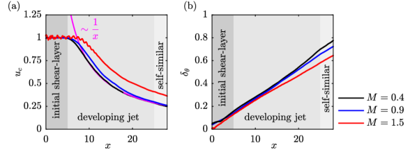
Figure 2: Mean flow characteristics for the three jets: (a) centerline velocity $u_{c}=\overline{u}_{x}(x,r=0)$; (b) momentum thickness $\delta_{\theta}=\int_{0}^{r_{1}}\frac{\bar{\rho}\bar{u}_{x}}{\rho_{c}u_{c}}\left(1-\frac{\bar{u}_{x}}{u_{c}}\right)\differential r$, where the integral is taken from the centerline to $r_{1}$ defined as $\bar{u}_{x}(r_{1})=\bar{u}_{\infty}+0.01\bar{u}_{j}$ (the $\bar{u}_{\infty}$ term is included to account for a small coflow included in the simulations). The centerline velocity becomes inversely proportional to the axial distance shortly after the potential core, and the momentum thickness increases approximately linearly.

The mean centerline velocity of the three jets is compared in figure 2(a). The plateau close to the nozzle characterizes the potential core, whose length increases with Mach number. A weak residual shock pattern is observed for $x\lesssim 10$ in the supersonic case. The streamwise development of turbulent jets is usually described in terms of an initial development region ($0\lesssim x/D\lesssim 25$), and a self-similar region ($x/D\gtrsim 25$), see e.g. Pope (2000). In the latter, the jet is fully described by a self-similar velocity profile, and a constant spreading and velocity-decay rate. For a dynamical description of the flow, we further divide the initial development region into two parts. The initial shear-layer region extends up to the end of the potential core ($0\lesssim x/D\lesssim 5$ for $M=0.4$) and is characterized by a constant velocity jump over the shear-layer, and a linearly increasing shear-layer thickness. The developing jet region lies between the end of the potential core and the start of the self-similar region ($5\lesssim x/D\lesssim 25$). In this region, the centerline velocity transitions rapidly to its asymptotic decaying behavior. The mean radial velocity profile, on the other hand, has not yet converged to its self-similar downstream solution. The $1/x$-scaling of the centerline velocity with streamwise distance (Pope, 2000) is indicated for the subsonic case. The momentum thickness shown in figure 2(b) increases approximately linear in all three regions in all cases. These characteristic velocities and length scales in each region imply different frequency scalings that will become important later.

Interpolated database								SPOD
case	$\frac{\Delta tc_{\infty}}{D}$	$n_{x}$	$n_{r}$	$n_{\theta}$	$x_{1}$	$r_{1}$	$n_{t}$	$n_{\text{freq}}$	$n_{\text{ovlp}}$	$n_{\text{blk}}$
subsonic	0.2	656	138	128	30	6	10,000	256	128	78
transsonic	0.2	656	138	128	30	6	10,000	256	128	78
supersonic	0.1	698	136	128	30	6	5,000	256	128	39

Table 2: Parameters of the structured cylindrical grid of the interpolated database (left), and the SPOD parameters (right).

In §§3-5, we will focus on the $M=0.4$ jet as the main conclusions are similar for all three Mach number regimes, and we address Mach number effects in detail in §6.

3 Spectral analysis of the LES data

In this section, we use spectral proper orthogonal decomposition (SPOD) to identify coherent structures within the three turbulent jets. This form of proper orthogonal decomposition (POD) identifies energy-ranked modes that each oscillate at a single frequency, are orthogonal to other modes at the same frequency, and, as a set, optimally represent the space-time flow statistics. SPOD was introduced by Lumley (1967, 1970) but has been used sparingly compared to the common spatial form of POD (Sirovich, 1987; Aubry, 1991) and dynamic mode decomposition (Schmid, 2010). However, recent work by Towne et al. (2017c) showed that SPOD combines the advantages of these other two methods–SPOD modes represent coherent structures that are dynamically significant and optimally account for the random nature of turbulent flows. This makes SPOD an ideal tool for identifying coherent structures within the turbulent jets considered in this paper.

We seek modes that are orthogonal in the inner product

$$\left<\boldsymbol{q}_{1},\boldsymbol{q}_{2}\right>_{E}=\iiint\boldsymbol{q}_{1}^{*}\mathrm{diag}\left(\frac{\overline{T}}{\gamma\overline{\rho}M^{2}},\overline{\rho},\overline{\rho},\overline{\rho},\frac{\overline{\rho}}{\gamma(\gamma-1)\overline{T}M^{2}}\right)\boldsymbol{q}_{2}r\differential x\differential r\differential\theta,$$ (2)

which are optimal in an induced compressible energy norm $\left<\cdot,\cdot\right>_{E}$ (Chu, 1965). The energy weights are defined for the state vector $\boldsymbol{q}=[\rho,u_{x},u_{r},u_{\theta},T]^{T}(x,r,\theta,t)$ of primitive variables density $\rho$, cylindrical velocity components $u_{x}$, $u_{r}$ and $u_{\theta}$, and temperature $T$. The notation $(\cdot)^{*}$ indicates the Hermitian transpose. We discretize the inner product defined by equation (2) as

$$\left<\boldsymbol{q}_{1},\boldsymbol{q}_{2}\right>_{E}=\boldsymbol{q}_{1}^{*}\mathsfbi{W}\boldsymbol{q}_{2},$$ (3)

where the weight matrix $\mathsfbi{W}$ accounts for both numerical quadrature weights and the energy weights. Since the jet is stationary and symmetric with respect to rotation about the jet axis, it can be decomposed into azimuthal Fourier modes $\hat{(\cdot)}_{m}$ of azimuthal wavenumber $m$, temporal Fourier modes $\hat{(\cdot)}_{\omega}$ of angular frequency $\omega$, or combined spatio-temporal Fourier modes Fourier modes $\hat{(\cdot)}_{m\omega}$ as

$$\boldsymbol{q}(x,r,\theta,t)=\sum_{m}\hat{\boldsymbol{q}}_{m}(x,r,t)\mathrm{e}^{\mathrm{i}m\theta}=\sum_{\omega}\hat{\boldsymbol{q}}_{\omega}(x,r,\theta)\mathrm{e}^{\mathrm{i}\omega t}=\sum_{m}\sum_{\omega}\tilde{\boldsymbol{q}}_{m\omega}(x,r)\mathrm{e}^{\mathrm{i}m\theta}\mathrm{e}^{\mathrm{i}\omega t}.$$ (4)

To calculate the SPOD, the data is first segmented into sequences $\boldsymbol{Q}=\left[\boldsymbol{q}^{(1)}\;\boldsymbol{q}^{(2)}\cdots\boldsymbol{q}^{(n_{\text{freq}})}\right]$ each containing $n_{\text{freq}}$ instantaneous snapshots of $\boldsymbol{q}$ which are considered to be statistically independent realizations of the flow under the ergodic hypothesis. Details on the interpolated databases and spectral estimation parameters are listed in table 2. The spatio-temporal Fourier transform of the $l$-th block yields $\hat{\boldsymbol{Q}}_{m\omega_{k}}^{(l)}=\left[\hat{\boldsymbol{q}}_{m\omega_{1}}^{(l)}\;\hat{\boldsymbol{q}}_{m\omega_{2}}^{(l)}\cdots\hat{\boldsymbol{q}}_{m\omega_{n_{\text{freq}}}}^{(l)}\right]$, where $\hat{\boldsymbol{q}}_{m\omega_{k}}^{(l)}$ is the $l$-th realization of the Fourier transform at the $k$-th discrete frequency. A periodic Hann window is used to minimize spectral leakage. The ensemble of $n_{\text{blk}}$ Fourier realizations of the flow at a given frequency $\omega_{k}$ and azimuthal wavenumber $m$ are now collected into a data matrix $\hat{\boldsymbol{Q}}_{m\omega_{k}}=\left[\hat{\boldsymbol{q}}_{m\omega_{k}}^{(1)}\;\hat{\boldsymbol{q}}_{m\omega_{k}}^{(2)}\cdots\hat{\boldsymbol{q}}_{m\omega_{k}}^{(n_{\text{blk}})}\right]$. For a particular $m$ and $\omega_{k}$, the SPOD modes are found as the eigenvectors $\boldsymbol{\Psi}_{m\omega_{k}}=\left[{\boldsymbol{\psi}}_{m\omega_{k}}^{(1)}\;{\boldsymbol{\psi}}_{m\omega_{k}}^{(2)}\cdots{\boldsymbol{\psi}}_{m\omega_{l}}^{(n_{\text{blk}})}\right]$, and the modal energy as the corresponding eigenvalues $\boldsymbol{\Lambda}_{m\omega_{k}}=\text{diag}\left(\lambda_{m\omega_{k}}^{(1)},\lambda_{m\omega_{k}}^{(2)},\cdots,\lambda_{m\omega_{k}}^{(n_{\text{blk}})}\right)$ of the weighted cross-spectral density matrix $\hat{\boldsymbol{S}}_{m\omega_{k}}=\hat{\boldsymbol{Q}}_{m\omega_{k}}\hat{\boldsymbol{Q}}_{m\omega_{k}}^{*}$ as

$$\hat{\boldsymbol{S}}_{m\omega_{k}}\boldsymbol{W}\boldsymbol{\Psi}_{m\omega_{k}}=\boldsymbol{\Psi}_{m\omega_{k}}\boldsymbol{\Lambda}_{m\omega_{k}}.$$ (5)

The modes are sorted by decreasing energy, i.e. $\lambda_{m\omega_{k}}^{(1)}\geq\lambda_{m\omega_{k}}^{(2)}\geq\cdots\geq\lambda_{m\omega_{k}}^{(n_{\text{blk}})}$. This formulation guarantees that the SPOD modes have the desired orthonormality property $\left<\boldsymbol{\psi}_{m\omega_{k}}^{(i)},\boldsymbol{\psi}_{m\omega_{k}}^{(j)}\right>_{E}=\delta_{ij}$, where $\delta_{ij}$ is the Kronecker delta function, and are optimal in terms of modal energy in the norm induced by equation (3). For brevity, we denote the $l$-th eigenvalue and the pressure component of the corresponding eigenmode as $\lambda_{l}$ and $\psi_{p}^{(l)}$, respectively. The dependence on a specific azimuthal wavenumber and frequency is implied and given in the description. Since the SPOD modes are optimal in terms of energy, we sometimes refer to the first SPOD mode as the leading or optimal mode and to the subsequent lower-energy modes as suboptimal modes.

Since we wish to express the data in terms of modes that oscillate at real and positive frequencies, we take the temporal Fourier transform in equation (4) first. Statistical homogeneity in $\theta$ implies that averaged quantities are the same for any $\pm m$. After verifying statistical convergence, we add the contributions of positive and negative $m$.

The distribution of power into the frequency components a signal is comprised of is referred to as its power spectrum. Power spectra are commonly expressed in terms of the power spectral density (PSD), which we will introduce later in equation (6). In the context of SPOD, we are interested in finding a graphical representation that can be interpreted in a similar way. In each frequency bin, the discrete SPOD spectrum is represented by the decreasing energy levels of the corresponding set of eigenfunctions. There is no obvious continuity in the modal structure of the most energetic mode (or any other) from one frequency bin to the next. Nevertheless, it is instructive to examine how the modal energy changes as a function of frequency, so that in what follows we plot the SPOD eigenvalues for each mode $l$ as functions $\lambda_{l}(\mbox{{St}})$ of frequency and refer to the resulting set of curves as the SPOD eigenvalue spectrum.

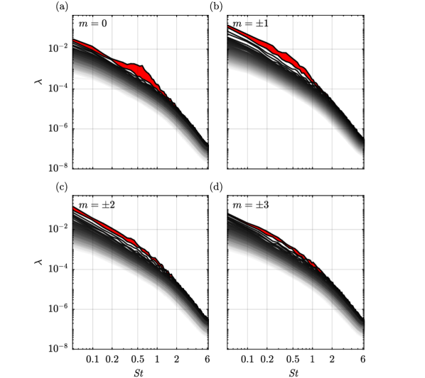
Figure 3: SPOD eigenvalue spectra ($\blacksquare\!{\color[rgb]{0.5,0.5,0.5}\blacksquare}\!\square$, $\lambda_{1}\!>\!\lambda_{2}\!>\!\cdots\!>\!\lambda_{N}$) for the subsonic jet: (a) $m=0$; (b) $m=1$; (c) $m=2$; (d) $m=3$. For, $m>0$, the positive and negative azimuthal wavenumber components are summed. Red shaded areas (${\color[rgb]{1,0,0}\blacksquare}$) highlight the separation between the first and second modes.

The SPOD eigenvalue spectrum of the axisymmetric component of the subsonic jet is shown in figure 3(a). The red shaded area highlights the separation between the first and second modes. A large separation indicates that the leading mode is significantly more energetic than the others. When this occurs, the physical mechanism associated with the first mode is prevalent, and we say that the flow exhibits low-rank behavior.

The low-rank behavior is apparent over the frequency band $0.2\lesssim\mbox{{St}}\lesssim 2$, and peaks at $\mbox{{St}}\approx 0.6$. It is most pronounced for $m=0$ and $m=1$, shown in panel 3(a) and 3(b), respectively. With increasing azimuthal wavenumber, the low-rank behaviour becomes less and less pronounced. For $m=1$, the dominance of the optimal gain persists to low frequencies, whereas it cuts off below $\mbox{{St}}\approx 0.2$ for $m=0$. For $m=2$ in figure 3(c), even though the eigenvalue separation is not very large, it is clear that the first resolvent mode at $St=0.2$ is a continuation of the same mode at higher frequencies. In contrast, the leading $m=0$ mode at $St=0.2$ appears to be a continuation of underlying band of the subpotimal SPOD modes. Since a global integral energy norm is used, it is important to note that the structure of the modes and their truncation by the domain unavoidably factor into the form of the energy spectra. These results should be compared with the optimal gain spectra shown in figure 8. The corresponding spectra for the transsonic and supersonic cases are reported in appendix A (figures 18 and 20).

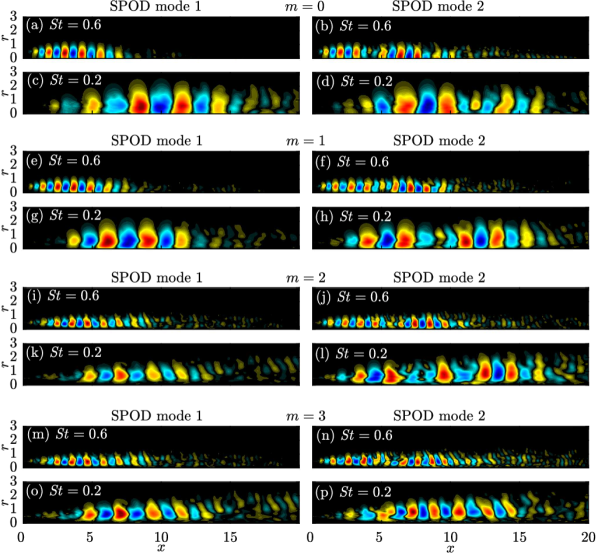
Figure 4: Comparison between SPOD mode 1 (left) and SPOD mode 2 (right) at two representative frequencies for the subsonic jet: (a-d) $m=0$; (e-h) $m=1$; (i-l) $m=2$; (m-p) $m=3$. The normalized pressure component (${\color[rgb]{1,0,0}\blacksquare}\!{\color[rgb]{0,0,0}\blacksquare}\!{\color[rgb]{0,0,1}\blacksquare}$, $-1<\psi_{p}/\|\psi_{p}\|_{\infty}<1$) is shown in $x,r\in[0\;20]\times[0\;3]$.

Figure 4 shows the first (left column) and the second (right column) SPOD modes at two representative frequencies and for $m=0,\dots,3$. The most energetic mode at $m=0$ and $\mbox{{St}}=0.6$ is shown in figure 4(a). These parameters correspond approximately to the point of maximum separation between the first and second mode in figure 3(a). The pressure field takes the form of a compact wavepacket in the initial shear-layer region of the jet (see figure 2). Its structure is reminiscent of the Kelvin-Helmholtz shear-layer instability of the mean flow (Suzuki & Colonius, 2006; Gudmundsson & Colonius, 2011; Jordan & Colonius, 2013). Crighton & Gaster (1976) argued that the mean flow can be regarded as an equivalent laminar flow, and found that it is convectively unstable (in the local weakly non-parallel sense) in the initial shear-layer region. Following their interpretation of this structure as a modal spatial instability wave, we refer to it as a KH-type wavepacket. The suboptimal SPOD mode shown in 4(b) has a double-wavepacket structure with an upstream wavepacket similar to the KH-type and a second wavepacket further downstream. This double-wavepacket structure is similarly observed at other frequencies and azimuthal wavenumbers, most prominently in figure 4(b,f,h,j,n). The turbulent mean flow in this region is convectively stable–it does not support spatial modal growth. Tissot et al. (2017) argue that the presence of large-scale structures in this region can be explained in terms of non-modal growth through the Orr mechanism. Our resolvent model presented in §4 supports this idea, and we therefore term these downstream or Orr-type wavepackets. Large parts of this paper are dedicated to establish a clear separation and explanation of these two distinct mechanisms.

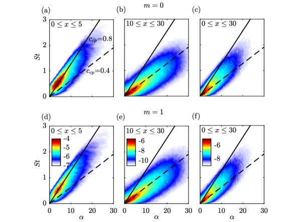
Figure 5: Frequency-wavenumber diagrams ($\square\!{\color[rgb]{0,1,1}\blacksquare}\!{\color[rgb]{1,0,0}\blacksquare}$, $\log_{10}(\bar{P}_{pp})$) of the subsonic simulation along the lip-line ($r=0.5$) over axial sections representative of the potential core (left column), downstream of the potential core (center column), and the entire jet (right column). The behaviors for $m=0$ (top row) and $m=1$ (bottom row) are similar. Two lines of constant phase speed ( , $c_{cp}=0.8$) and (     , $c_{cp}=0.4$) are shown as a reference. Rows share the same contour levels.

In order to further isolate mechanisms associated with different regions of the jet, we construct empirical frequency-wavenumber diagrams by taking the Fourier transform in the streamwise direction of the LES pressure along the lip line ($r=0.5$). We compute the spatio-temporal PSD as

$$\bar{P}_{qq}=\frac{1}{n_{\text{blk}}}\sum_{l=1}^{n_{\text{blk}}}\left|\hat{q}^{(l)}_{m\omega\alpha}\right|^{2},$$ (6)

where $\hat{(\cdot)}_{\alpha}$ is the Fourier transform in the axial direction and $\alpha$ the axial wavenumber. In figure 5, the PSD is plotted, and compared to the PSD computed with different window functions constraining the signal to specific regions along the streamwise axis, specifically $0\leq x\leq 5$, representing the annular shear layer, and $10\leq x<30$, the developing jet.

Qualitatively similar results are found for $m=0$ (top row) and $m=1$ (bottom row). In the initial shear layer region investigated in figure 5a and 5d, the pressure PSD follows the line of constant phase speed $c_{ph}=0.8$ and peaks at $\mbox{{St}}\approx 0.5$ for $m=0$, and a slightly lower frequency for $m=1$. This phase speed is typical for KH-type shear-layer instability waves, and the peak frequencies are close to the ones where the low-rank behavior is most pronounced in figure 3a and 3b, respectively. In the developing jet region in figure 5b and 5e, waves propagate with about half of the phase speed observed in the initial shear-layer, and the PSD peaks at the lowest resolved frequency. The PSD for the entire domain shown in figure 5c and 5f, by construction, combines these effects.

4 Resolvent model

A key concept that emerged from the early studies of transient growth (Farrell & Ioannou, 1993; Trefethen et al., 1993; Reddy et al., 1993; Reddy & Henningson, 1993) is that of the resolvent operator. The resolvent operator is derived from the forced linearized equations of motion and constitutes a transfer function between body forces and corresponding responses. It has been used to study the linear response to external forcing of a range of laminar flows including channel flow (Jovanović & Bamieh, 2005; Moarref & Jovanović, 2012), boundary layers (Monokrousos et al., 2010; Sipp & Marquet, 2013) and the flow over a backward-facing step (Dergham et al., 2013).

When the resolvent is computed for the turbulent mean flow, the forcing can be identified with the nonlinear effects, namely the triadic interactions that conspire to force a response at a given frequency and azimuthal wavenumber (McKeon & Sharma, 2010). Previous resolvent analyses of turbulent jets include those of jets Garnaud et al. (2013), Jeun et al. (2016) and Semeraro et al. (2016).

The use of a resolvent model is motivated by recent findings that connect SPOD and resolvent analysis (Towne et al., 2015; Semeraro et al., 2016; Towne et al., 2017c). Specifically, SPOD and resolvent modes are identical when the SPOD expansion coefficients are uncorrelated, which is typically associated with white-noise forcing.

4.1 Methodology

We start by writing the forced linear governing equations, here the compressible Navier-Stokes equations, as an input-output system in the frequency domain

$$\left(-\mathrm{i}\omega\mathsfbi{I}-\mathsfbi{A}_{m}\right)\hat{\boldsymbol{q}}_{m\omega} = \mathsfbi{B}\hat{\boldsymbol{f}}_{m\omega},$$ (7)

$$\hat{\boldsymbol{y}}_{m\omega} = \mathsfbi{C}\hat{\boldsymbol{q}}_{m\omega},$$ (8)

where $\mathsfbi{A}_{m}$ is the linearized compressible Navier-Stokes operator, $\hat{\boldsymbol{q}}_{m\omega}$ is the state vector as before, and $\hat{\boldsymbol{f}}_{m\omega}$ the (for now unspecified) forcing. Equation (8) defines the output, or response, $\hat{\boldsymbol{y}}_{m\omega}$ as the product of an output matrix $\mathsfbi{C}$ with the state. Analogously, a input matrix $\mathsfbi{B}$ is introduced in (7). Without forcing, the right hand side of equation (7) is zero, and the global linear stability eigenvalue problem for $\hat{\boldsymbol{q}}_{m\omega}$ and $\omega$ is recovered. We use the same discretization scheme as in Schmidt et al. (2017) and refer to that paper for details on the numerical method.

Equations (7) allow us to express a direct relation between inputs and outputs,

$$\hat{\boldsymbol{y}}_{m\omega}=\mathsfbi{H}_{m\omega}\hat{\boldsymbol{f}}_{m\omega},$$ (9)

by defining the resolvent operator

$$\mathsfbi{H}_{m\omega}=\mathsfbi{C}\left(-\mathrm{i}\omega\mathsfbi{I}-\mathsfbi{A}_{m}\right)^{-1}\mathsfbi{B}$$ (10)

as the transfer function between them. We further define the modified, or weighted, resolvent operator

$$\mathsfbi{R}_{m\omega}=\mathsfbi{W_{y}}^{\frac{1}{2}}\mathsfbi{H}_{m\omega}\mathsfbi{W_{f}}^{-\frac{1}{2}}=\tilde{\mathsfbi{Y}}\boldsymbol{\Sigma}\tilde{\mathsfbi{F}}^{*}$$ (11)

that account for arbitrary inner products on the input and output spaces that are defined shortly. In the last equality of equation (11), we anticipated the result that the optimal responses $\tilde{\mathsfbi{Y}}=[\tilde{\boldsymbol{y}}_{m\omega}^{(1)}\;\tilde{\boldsymbol{y}}_{m\omega}^{(2)}\cdots\tilde{\boldsymbol{y}}_{m\omega}^{(N)}]$, forcings $\tilde{\mathsfbi{F}}=[\tilde{\boldsymbol{f}}_{m\omega}^{(1)}\;\tilde{\boldsymbol{f}}_{m\omega}^{(2)}\cdots\tilde{\boldsymbol{f}}_{m\omega}^{(N)}]$, and amplidude gains $\boldsymbol{\Sigma}=\text{diag}\left(\sigma_{1},\sigma_{2},\cdots,\sigma_{N}\right)$ can be found from the singular value decomposition (SVD) of the modified resolvent operator. By $\tilde{(\cdot)}$ we denote singular or eigenvectors. The modified resolvent operator in equation (11) is weighted such that the orthonormality properties

$$\left<\tilde{\boldsymbol{y}}_{m\omega}^{(i)},\tilde{\boldsymbol{y}}_{m\omega}^{(j)}\right>_{y} = \tilde{\boldsymbol{y}}_{m\omega}^{(i)^{*}}\mathsfbi{W_{y}}\tilde{\boldsymbol{y}}_{m\omega}^{(j)}=\delta_{ij}\text{ and}$$ (12)

$$\left<\tilde{\boldsymbol{f}}_{m\omega}^{(i)},\tilde{\boldsymbol{f}}_{m\omega}^{(j)}\right>_{f} = \tilde{\boldsymbol{f}}_{m\omega}^{(i)^{*}}\mathsfbi{W_{f}}\tilde{\boldsymbol{f}}_{m\omega}^{(j)}=\delta_{ij}$$ (13)

hold for the optimal responses in the output norm $\left<\cdot,\cdot\right>_{y}$, and the forcings in the input norm $\left<\cdot,\cdot\right>_{f}$, respectively. The optimal forcings and responses are found from the definition of the optimal energetic gain

$$G^{2}_{max}(\hat{\boldsymbol{f}}_{m\omega})=\max_{\|\hat{\boldsymbol{f}}_{m\omega}\|^{2}_{f}=1}\frac{\big{<}\hat{\boldsymbol{y}}_{m\omega},\hat{\boldsymbol{y}}_{m\omega}\big{>}_{y}}{\big{<}\hat{\boldsymbol{f}}_{m\omega},\hat{\boldsymbol{f}}_{m\omega}\big{>}_{f}}=\frac{\big{<}\tilde{\boldsymbol{y}}_{m\omega},\tilde{\boldsymbol{y}}_{m\omega}\big{>}_{y}}{\big{<}\tilde{\boldsymbol{f}}_{m\omega},\tilde{\boldsymbol{f}}_{m\omega}\big{>}_{f}}=G^{2}(\tilde{\boldsymbol{f}}_{m\omega}^{(1)})=\sigma_{1}^{2}$$ (14)

between inputs and outputs (see Schmid & Henningson, 2001). By writing the energetic gain in form of a generalized Rayleigh quotient and inserting equations (9) and (10), it is found that the orthogonal basis of forcings optimally ranked by energetic gain can be found from the eigenvalue problem

$$\mathsfbi{W_{f}}^{-1}\mathsfbi{B}^{H}\left(-\mathrm{i}\omega\mathsfbi{I}-\mathsfbi{A}_{m}\right)^{-H}\mathsfbi{C}^{H}\mathsfbi{W_{y}}\mathsfbi{C}\left(-\mathrm{i}\omega\mathsfbi{I}-\mathsfbi{A}_{m}\right)^{-1}\mathsfbi{B}\tilde{\boldsymbol{f}}_{m\omega}^{(i)}=\sigma^{2}_{i}\tilde{\boldsymbol{f}}_{m\omega}^{(i)}.$$ (15)

Equation (17) is solved by first factoring $\left(-\mathrm{i}\omega\mathsfbi{I}-\mathsfbi{A}_{m}\right)=\mathsfbi{L}\mathsfbi{U}$ (Sipp & Marquet, 2013) and then solving the eigenvalue problem

$$\mathsfbi{W_{f}}^{-1}\mathsfbi{B}^{H}\mathsfbi{U}^{-H}\mathsfbi{L}^{-H}\mathsfbi{C}^{H}\mathsfbi{W_{y}}\mathsfbi{C}\mathsfbi{U}^{-1}\mathsfbi{L}^{-1}\mathsfbi{B}\tilde{\mathsfbi{F}}=\tilde{\mathsfbi{F}}\boldsymbol{\Sigma}^{2}$$ (16)

for the largest eigenvalues using a standard Arnoldi method. The corresponding responses are readily obtained as

$$\tilde{\mathsfbi{Y}}=\mathsfbi{R}_{m\omega}\tilde{\mathsfbi{F}}=\mathsfbi{W_{y}}^{\frac{1}{2}}\mathsfbi{C}\mathsfbi{U}^{-1}\mathsfbi{L}^{-1}\mathsfbi{B}\mathsfbi{W_{f}}^{-\frac{1}{2}}\tilde{\mathsfbi{F}}.$$ (17)

In this study, we quantify both the energy of the input and the output in the compressible energy norm, as defined in equation (3), by setting $\mathsfbi{W_{y}}=\mathsfbi{W_{f}}=\mathsfbi{W}$. The matrices $\mathsfbi{B}$ and $\mathsfbi{C}$ we use for the sole purpose of restricting the analysis to the physical part of the computational domain by assigning zero weights to the sponge region. The physical domain corresponds to the domain of the LES data detailed in table 2. It is surrounded by a sponge region of width $D$, and discretized using $950\times 195$ points in the streamwise and radial direction, respectively. The streamwise extent of the domain sets a limit of $\mbox{{St}}\gtrsim 0.2$ on the lowest possible frequency. For lower frequencies, the response structures become so elongated that domain truncation affects the gain. An upper limit on St is imposed by the numerical discretization, i.e. the capability of the differentiation scheme to resolve the smallest structures in the response and forcing fields for the given resolution. This limit is $\mbox{{St}}\lesssim 2.5$ for the subsonic, $\mbox{{St}}\lesssim 1.5$ for the transsonic, and $\mbox{{St}}\lesssim 1$ for the supersonic case, respectively. A molecular Reynolds number of $\Rey=3\cdot 10^{4}$ is used for this study. We return to this issue later and discuss our rationale in §4.3.

4.2 Resolvent spectra and modes

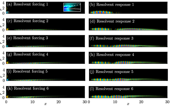
Figure 6: Optimal and suboptimal resolvent forcings (left) and corresponding responses (right) of the subsonic jet for $St=0.6$ and $m=0$. The pressure field (${\color[rgb]{1,0,0}\blacksquare}\!{\color[rgb]{0,0,0}\blacksquare}\!{\color[rgb]{0,0,1}\blacksquare}$) is normalized with respect to its maximum absolute value. The optimal response mode in (a) is of KH type, whereas all suboptimal modes combine the KH and Orr-type waves. The inset in panel (a) shows the forcing structure close to the nozzle. The shear-layer and the potential core are outlined as in figure 1.

Figure 6 shows the optimal and the five leading suboptimal forcings and responses for $St=0.6$ and $m=0$. The leading mode in figure 6(b) resembles a KH-type instability wavepacket that is confined to the initial shear-layer region. The corresponding optimal forcing in figure 6(a) is confined close to the nozzle. The insert in figure 6(a) reveals that the KH-type wavepacket is most efficiently forced by a structure that is oriented against the mean-shear in the vicinity of the lip-line. This is a typical manifestation of the Orr-mechanism and has similarly been observed in resolvent models of other flows (in Garnaud et al., 2013; Dergham et al., 2013; Jeun et al., 2016; Semeraro et al., 2016; Tissot et al., 2017). The suboptimal modes in figure 6(d,f,h,j,l) contain two wavepackets: one in the initial shear layer region that is similar to the KH wavepackets in the optimal mode and a second further downstream in the developing jet region. With increasing mode number, the downstream wavepacket moves upstream and becomes more spatially confined. It is optimally forced downstream of the inlet and over an axial distance comparable to the length of the response. Following the same arguments as for the suboptimal SPOD modes presented in figure 4, we term the downstream wavepackets Orr-type wavepackets. Both the KH-type and the Orr-type wavepackets are optimally exerted via the Orr-mechanism. From a local stability theory point of view, the two mechanisms are distinguished by their modal and non-modal nature, see Jordan et al. (2017) and Tissot et al. (2017)).

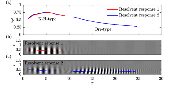
Figure 7: The critical layer effect in the subsonic jet for $St=0.6$ and $m=0$: (a) estimated phase velocity (  first mode;   second mode); (b,c) normalized pressure of the first and second mode ($\blacksquare\!{\color[rgb]{0.5,0.5,0.5}\blacksquare}\!\square$), and critical layer location where $c_{ph}=\bar{u}_{x}$. The KH and Orr wavepackets clearly follow the critical layer.

Tissot et al. (2017) found that the critical layer, defined where the phase speed of the wavepacket is equal to the local mean velocity, plays an important role in the forced linear dynamics of jets. In accordance with our interpretation, their results suggests that the Orr-mechanism is active downstream of the potential core. Figure 7(a) shows the phase velocity of the leading and first suboptimal resolvent response for $m=0$ and $\mbox{{St}}=0.6$. The phase velocity is approximated as $c_{ph}\approx\omega/\frac{\partial\theta_{p}}{\partial x}$, where $\theta_{p}=\arg(\phi_{p})$ is the local phase of the pressure along $r=0.5$. The phase velocity is plotted for the regions where the pressure exceeds 25% of its global absolute maximum value. The phase velocity of the upstream wavepacket in the initial shear-layer is almost identical for the first and second response mode. Besides their similar structure, this also suggests that the primary wavepacket of the suboptimal mode is of KH-type. The phase velocity of the downstream wavepacket decreases with axial distance in accordance with the jet’s velocity-decay rate. Panels 7(b,c) show that the first and second wavepackets closely follow the critical layer. The variation of the phase speed with axial distance explains why the KH and Orr wavepackets are characterized by broad bands in frequency-wavenumber space, see figure 5.

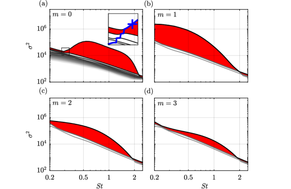
Figure 8: Optimal energetic gain spectra ($\blacksquare\!{\color[rgb]{0.5,0.5,0.5}\blacksquare}\!\square$, $\sigma_{1}\!>\!\sigma_{2}\!>\!\cdots\!>\!\sigma_{N}$) for the subsonic jet: (a) $m=0$; (b) $m=1$; (c) $m=2$; (d) $m=3$. The difference between the optimal and the first suboptimal mode (${\color[rgb]{1,0,0}\blacksquare}$) highlights the low-rank behavior. The thirty largest singular values were computed for $m=0$, and the three largest for $m>0$. In the inset in panel (a), the KH-type mode is tracked ( ) into the frequency range where it becomes suboptimal. The leading mode at $\mbox{{St}}=0.33$ (${\color[rgb]{0,0,1}\boldsymbol{+}}$) serves reference and the scalar projection $\langle\boldsymbol{q}^{(i)},\boldsymbol{q}^{(1)}_{\text{ref}}\rangle_{E}$ onto that mode is used for the tracking.

Resolvent gain spectra for the first four azimuthal wavenumbers are shown figure 8. As in figure 3, we highlight the difference between the leading and the first suboptimal gain to emphasize low-rank behavior. A pronounced low-rank behavior is evident for $0.3\lesssim\mbox{{St}}\lesssim 2$ for $m=0$ as can be seen in panel 8(a). The 20 leading modes were calculated for $m=0$, and the the three leading modes for $m>0$. The inset in panel 8(a) shows that the KH mechanism persists into lower frequencies as a suboptimal mode ( ). The reference mode is of pure KH-type, and it was confirmed by visual inspection of the mode shapes (not shown) that the KH signature indeed prevails in the suboptimal modes. The vertical line segments indicate where transitions to the next lower singular suboptimal. At high frequencies, the continuation is more obvious. For all four azimuthal wavenumbers, the curve associated with the KH wavepacket crosses the suboptimal gain curves at $\mbox{{St}}\approx 2$. This marks the end of the low-rank frequency band. For $m>0$, the low-rank band extends to lower frequencies. Panel 8(b) shows that a strong low-rank behavior is predicted for frequencies even lower that the minimum frequency $\mbox{{St}}<0.2$ for $m=1$. With increasing azimuthal wavenumber, the low-rank behavior becomes less and less pronounced. All these qualitative trends are reflected in the empirical SPOD energy spectra in figure 3. The direct comparison of the SOPD analysis with the resolvent model is the subject of §6.

4.3 Reynolds number effects

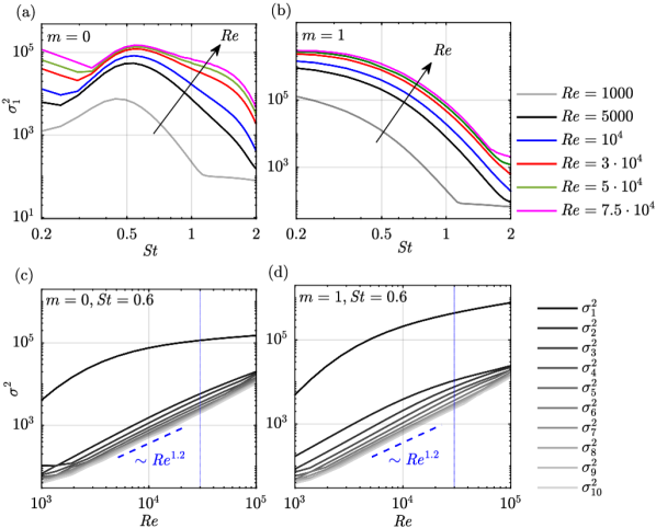
Figure 9: Reynolds number effect on the energetic gain of the subsonic jet: (a,b) optimal gain spectra for $m=0$ and $m=1$; (c,d) energetic gain at $\mbox{{St}}=0.6$ for $m=0$ and $m=1$. The blue dotted line (${\color[rgb]{0,0,1}\cdots}$) marks the Reynolds number $\Rey=3\cdot 10^{4}$ used for the present study.

The effect of the Reynolds number on the spectrum of the discretized linearized Navier-Stokes operator $\mathsfbi{A}_{m}$ is studied in Schmidt et al. (2017, appendix D). In figure 9, the effect of the Reynolds number on the resolvent gain is investigated. The optimal gain $\sigma_{1}^{2}$ for $m=0$ and $m=1$ shown in panels 9(a) and 9(b), respectively, increases with increasing Reynolds number over the entire frequency range. Above $\Rey\geq 3\cdot 10^{4}$, the gain does not show a pronounced dependency on the Reynolds number for all but the lowest frequencies for $m=0$. The gain of the leading ten modes at a fixed frequency of $\mbox{{St}}=0.6$ is shown below in 9(c,d). At this particular frequency, the optimal gain is significantly higher that the suboptimal gains, which are all of comparable magnitude. Similar to the modal energy gap in the SPOD analysis, this reflects the low-rank behavior of the jet in the resolvent model. The suboptimal gains follow an approximate power law behavior over the range of Reynolds number studied. The different behavior of the optimal and the suboptimal gains highlights the disparate physical nature of the two mechanisms. Their different scalings highlight the importance of a proper choice of Reynolds number for mean-flow-based resolvent models. In particular, the model Reynolds number determines which of the two mechanisms dominates at a certain frequency. This becomes apparent, for example, for $m=0$ at low frequencies: the kink in the gain curves in figure 9(a), which marks the transition from one scaling to another, shifts to higher frequencies with increasing Reynolds number. For $\Rey=7.5\cdot 10^{4}$, the exchange of optimal mechanisms occurs at $\mbox{{St}}\approx 0.35$, whereas it occurs at $\mbox{{St}}\approx 0.25$ for $\Rey=7.5\cdot 10^{4}$. We chose a Reynolds number of $\Rey=3\cdot 10^{4}$ for the present study. This choice is motivated by the good correspondence with the LES, as discussed in the next section. For now, and in absence of a proper model for the effective Reynolds number, the Reynolds number has to be understood as a free model parameter. Mettot et al. (2014), for example, demonstrate that resolvent analyses based on the linearized Reynolds-averaged Navier-Stokes (RANS) equations with modeled turbulence do not necessarily give superior results to our ad-hoc approach.

5 Comparison of the SPOD and resolvent models

In this section, we make comparisons between the high-energy SPOD modes and the high-gain resolvent modes. This comparison is facilitated by recently established theoretical connections between the two methods (Towne et al., 2015; Semeraro et al., 2016; Towne et al., 2017c). Specifically, the resolvent operator relates the cross-spectral density of the nonlinear forcing to the cross-spectral density of the response. IF the forcing were uncorrelated in space and time with equal amplitude everywhere, i.e., unit-variance white noise, then the SPOD and resolvent modes would be identical. This result is conceptually intuitive–when there is no bias in the forcing, the modes with highest gain are also the most energetic.

The nonlinear forcing terms in real turbulent flows are, of course, not white. Zare et al. (2017) showed that it is necessary to account for correlated forcing in order to reconstruct the flow statistics of a turbulent channel flow using a linear model. Of particular relevance to our study, Towne et al. (2017a) investigated the statistical properties of the nonlinear forcing terms in a turbulent jet. They found limited correlation in the near-nozzle shear-layer but significant correlation further downstream, especially near and beyond the end of the potential core.

Correlated nonlinear forcing leads to differences between SPOD and resolvent modes. Precisely, the correlation causes a bias in the forcing that preferentially excites certain resolvent modes and mixes them together via correlations between different modes (Towne et al., 2017c). As a result, multiple resolvent modes are required to reconstruct each SPOD mode. Accordingly, we do not expect a one-to-one correspondence between the SPOD and resolvent modes of the jet. Rather, we are looking for the signatures of the high-gain resolvent modes within the high-energy SPOD modes. That is, we seek evidence that the mechanisms identified in the resolvent modes are active in the real flow and responsible for the most energetic coherent structures.

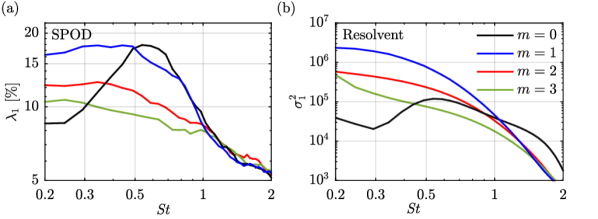
Figure 10: First SPOD mode energy spectra (a) and optimal resolvent gain (b) for $0\leq m\leq 3$ for the subsonic jet. A five-point moving average filter was used to increase the clarity of the SPOD spectrum.

The leading mode SPOD energy spectra (see figure 3) and optimal resolvent gain curves (see figure 8) for $m=0,\cdots,3$ are compared in figure 10. In panel 10(a), we show the relative energy of the leading mode in percentages of the total energy at each frequency. We choose this quantity as a qualitative surrogate for the gain, which is not defined for the LES data. The resolvent gain curves capture the trends of the SPOD eigen-spectra remarkably well. The peak in relative energy of the leading $m=0$ SPOD mode in figure 10(a) clearly indicates low-rank behavior. At low frequencies, the ordering of the resolvent gains is directly reflected in the relative importance of the corresponding SPOD modes.

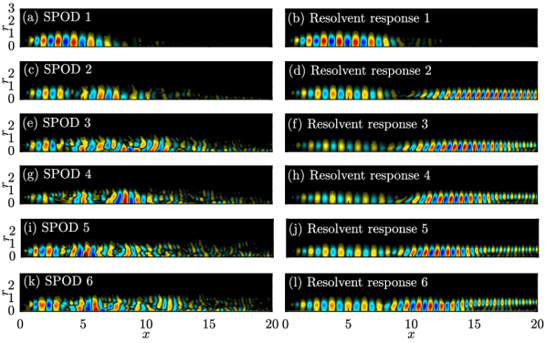
Figure 11: Empirical SPOD modes (left) and optimal resolvent response modes (right) for $St=0.6$ and $m=0$ for the subsonic jet. The normalized pressure is shown. The leading resolvent response in (b) accurately models leading SPOD mode in (a).

A comparison of the six leading resolvent and SPOD modes for $m=0$ and $\mbox{{St}}=0.6$ is shown in figure 11. The KH-type wavepacket of the first SPOD mode in 11(a) closely resembles the optimal resolvent mode in figure 11(b). Unlike the resolvent responses (as discussed in the context of figure 6), the subdominant SPOD modes do not follow an immediately obvious hierarchy. Similar to the resolvent modes, they exhibit a multi-lobe structure and peak downstream or at the end of the potential core. Close to the nozzle, their structure resembles the KH-type waveform of the first mode. Their highly distorted structure suggests that their statistics may not be as well converged as the leading mode. The first three modes are characterized by an increasing integer number of lobes or successive wavepackets (this becomes much more evident in figure 14 below).

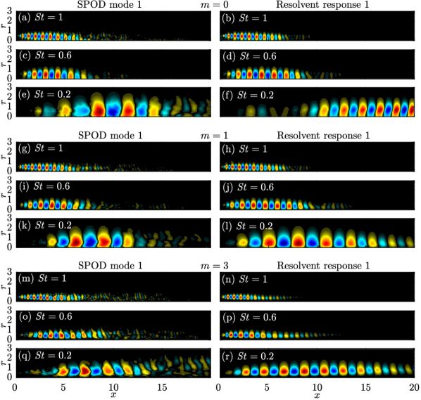
Figure 12: Comparison between leading empirical SPOD modes (left) and optimal resolvent response modes (right) at three representative frequencies for the subsonic jet: (a-f) $m=0$; (g-l) $m=1$; (m-r) $m=3$. The normalized pressure is shown. The leading modes compare favorably with the exception of the low frequency case for $m=0$ shown in (e,f), where the SPOD mode is of KH type, whereas the optimal response mode is of Orr type. Only part of the computational domain is shown for clarity.

Figure 12 makes direct comparisons between the leading SPOD and resolvent modes for different frequencies ($\mbox{{St}}=1.0,0.6,0.2$) and azimuthal wavenumbers ($m=0,1,3$). In general, the modes compare well for frequency-azimuthal wavenumber combinations that exhibit low-rank behavior according to the SPOD and resolvent gain spectra in figures 3 and 8, respectively. For example, good agreement is obtained for $\mbox{{St}}=0.6$ and $\mbox{{St}}=1.0$ for $m=0$ and $m=1$, i.e. figure 12(a-d,g-j). In figure 12(e,f), the leading resolvent mode is an Orr-type wavepacket far downstream of the potential core, whereas the SPOD mode peaks further upstream and has a larger axial wavelength. For $m=3$ in figure 12(m-q) and higher azimuthal wavenumbers, the SPOD modes appear to be less well converged as compared to their low $m$ counterparts. This is, again, explained by the observation that the low-rank behavior decreases as $m$ increases.

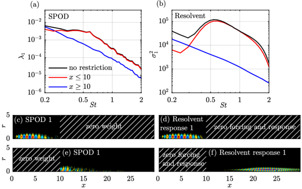
Figure 13: Isolation of the mechanisms for spatial modal growth in the initial shear layer, and non-modal spatial growth further downstream for the subsonic jet: (a) SPOD spectra; (b) optimal resolvent gain spectra; (c-f) normalized pressure field for $St=0.6$. For the SPOD, the restriction is realized via the weight matrix and the non-zero weighted regions are shown. For the resolvent analysis, the forcing and response are restricted via the input and output matrices.

Both the SPOD and resolvent methodologies allow us to isolate the characteristics of the KH-type wavepackets near the nozzle and the downstream Orr-type wavepackets through their different spatial support. In the SPOD analysis, we utilize the weight matrix $\mathsfbi{W}$ to assign zero weight to the region we wish to exclude, e.g. $x>10$, to focus on the initial shear-layer region and vice versa for the developing jet region. The resulting energy spectra and modes are depicted in figure 13(a,c,e). For the resolvent analysis, we restrict both the forcing and the response to the region of interest through the input and output matrices $\mathsfbi{B}$ and $\mathsfbi{C}$. The resulting gain spectra and modes are shown in figure 13(b,d,f). The SPOD and gain spectra consistently separate the two mechanisms. In both cases, the spectra obtained without spatial restriction are a superposition of the spectra of the two isolated physical mechanisms. The different spatial support of the restricted SPOD (panel 13(e)) and resolvent (panel 13(f)) modes emphasizes that the forcing of the subdominant mode is clearly not white, though there are obvious similarities in the wavepacket shape indicating a similar mechanism.

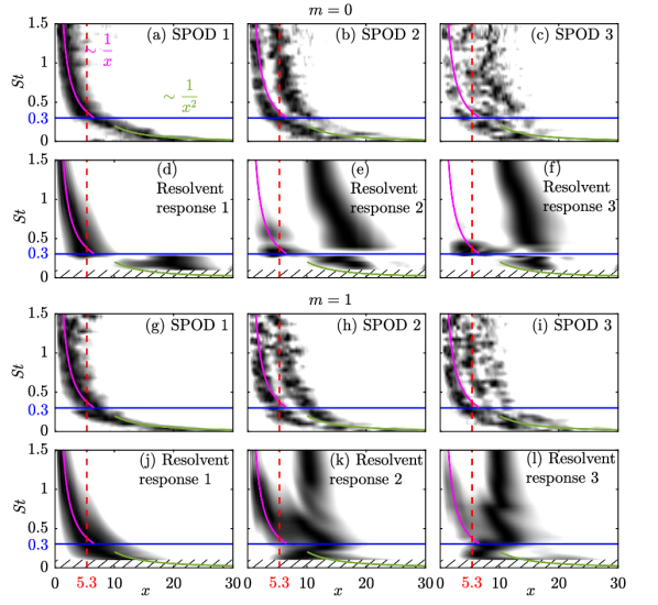
Figure 14: Frequency-axial distance diagrams ($\blacksquare\!{\color[rgb]{0.5,0.5,0.5}\blacksquare}\!\square$,$\tilde{P}_{pp}$) along the lip-line ($r_{0}=0.5$) for $m=0$ (top half) and $m=1$ (bottom half) for the subsonic jet. The three leading SPOD and resolvent modes are compared. The estimated pressure PSD, $\bar{P}_{pp}$, is normalized by its maximum value at each frequency. The end of the potential core (      , $x=5.3$), and a Strouhal number of $\mbox{{St}}=0.3$ (  ) differentiate shear-layer from developing jet behavior. The different frequency scalings of shear-layer (  , $\mbox{{St}}\sim\frac{1}{x}$) and jet wavepackets (  , $\mbox{{St}}\sim\frac{1}{x^{2}}$) are indicated.

Plotting the temporal and azimuthal PSD

$$\tilde{P}_{qq}=\frac{1}{n_{\text{blk}}}\sum_{l=1}^{n_{\text{blk}}}\left|\hat{q}^{(l)}_{m\omega}(x,r=r_{0})\right|^{2}$$ (18)

as a function of $x$ along a line of constant distance $r_{0}$ from the axis allows us to locate the wavepackets in space. The resulting frequency-axial distance diagrams are shown in figure 14 for $m=0$ and $m=1$. The results for the SPOD and the resolvent response modes are directly compared. This form of visualization of the SPOD modes brings to light the hierarchal structure of the SPOD modes more clearly. From figure 12a-c for $m=0$, and 12g-i for $m=1$, respectively, it becomes apparent that the higher order modes are characterized by an increasing number of subsequent wavepackets in the streamwise direction.

The change from KH-type shear-layer instability to Orr-type wavepackets in the developing jet is apparent from the change of the slope of the PSD at $(x,\mbox{{St}})\approx(6,0.3)$. Different frequency scalings in the two regions explain this sudden change. They can be directly deduced from the varying characteristic velocity and length scales of each region as shown in figure 2. The initial shear-layer grows linearly while the characteristic velocity stays constant. The frequency of the high-frequency wavepackets therefore scales with $1/x$. In the developing and self-similar jet regions, the jet width increases linearly, but the centerline velocity decays inversely proportional to the axial distance. The frequency in that region consequentl y scales with $1/x^{2}$. The different frequency-scalings in the two regions of the jet are apparent in other studies on wavepacket modeling (Cavalieri et al., 2016; Sasaki et al., 2017), and on acoustic-source localization (Bishop et al., 1971; Schlinker et al., 2009).

The optimal response modes in figure 14(d) and 14(j) accurately predict the wavepacket location in the initial shear-layer region in the leading SPOD modes. For $m=1$ in figure 14(j), the low-rank behavior of the jet permits accurate predictions at low frequencies. For $m=0$ (panel 14(d)), on the contrary, the non-low-rank behavior at low frequencies hinders a rank-one resolvent-mode representation of the leading SPOD mode. Similarly, the subdominant SPOD modes shown in panels 14(b,c) and 14(h,i) cannot be represented by a single suboptimal resolvent mode.

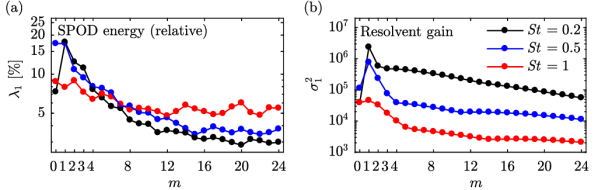
Figure 15: Azimuthal wavenumber dependence of the relative modal energy of the SPOD (a), and the optimal resolvent gain (b) for three representative frequencies fir the subsonic jet.

The azimuthal wavenumber dependence of the SPOD energy and the resolvent gain is investigated in figure 15. As in figure, 10, we show the percentage of the energy of the first SPOD mode to highlight low-rank behavior. The falloff of the SPOD energy spectra seen in panel 15(a) implies that the low-rank behavior is more pronounced at low azimuthal wavenumbers and lower frequencies. For higher frequencies such as $\mbox{{St}}=1$, the relative energy of the first SPOD mode is not a strong function of the azimuthal wavenumber. At higher azimuthal wavenumbers $m\gtrsim 10$, its relative energy content stays at $\approx 5\%$, which is above the levels of the two lower frequency cases. Similar trends are observed for the resolvent gain shown in panel 15(b). The maximum gain, for example, is attained for $m=1$, and the gain curve for the highest frequency is a much weaker function of the azimuthal wavenumber than in the case of two lower frequencies. For higher azimuthal wavenumbers, the gain falls off almost monotonically.

6 Effect of the Mach number

In the following, we addresses the effect of compressibility on the low-rank behavior. SPOD and resolvent analyses are conducted for the other two LES cases with $M_{j}=0.9$ and $M_{j}=1.5$, respectively (see table 1). The main conclusions drawn from the analysis of the subsonic case in §§3-4 regarding the behavior of the KH- and Orr-type wavepackets apply to the other regimes as well. We therefore catalogue the complete results for the two additional higher Mach number cases in appendix A, and focus on specific Mach number dependent physical effects in this section.

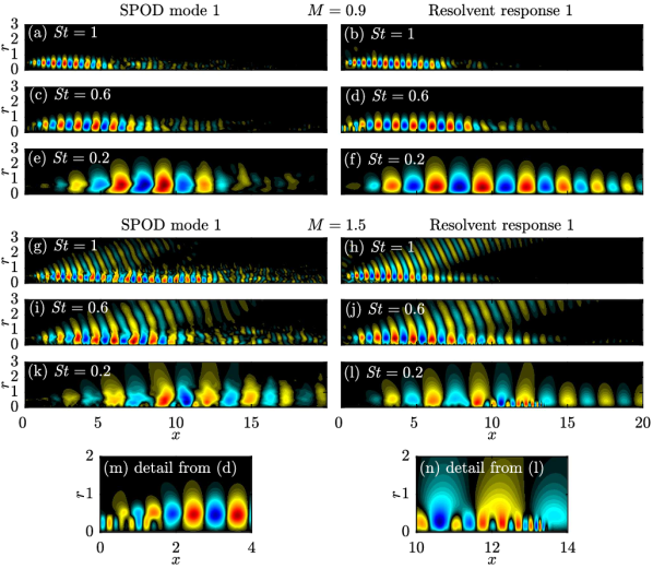
Figure 16: Comparison between leading empirical SPOD modes and optimal resolvent response modes at three representative frequencies for $m=1$ for the transsonic (a-f) and the supersonic jet (g-l). Panels (m) and (n) zoom in on a trapped acoustic mode (Towne et al., 2017b; Schmidt et al., 2017) in the transonic jet, and an upstream-propagating subsonic mode (Tam & Hu, 1989) in the supersonic jet, respectively. The normalized pressure is shown.

Figure 16 shows a side-by-side comparison of SPOD and resolvent modes for the transsonic and the supersonic jet. The leading modes are shown for three frequencies. Similar to the subsonic case in figure 12, favorable agreement between the empirical modes and the model is found. Significant discrepancies in terms of the length of the wavepackets and their radial structure is only observed for the transsonic jet at the lowest frequency, as shown in panels 16(e,f). In panels 16(g-j), it can be seen that the resolvent model accurately predicts the super-directive Mach wave radiation of the supersonic jet. Sinha et al. (2014) found similarly good agreement with their PSE model.

Besides the KH and Orr-type wavepackets, which are vortical, jets also support different types of frequency-dependent acoustic waves. The transsonic jet, for example, supports trapped acoustic waves within the potential core (Towne et al., 2017b; Schmidt et al., 2017). Such a trapped acoustic wave can be seen close to the nozzle in the detail shown in panel 16(m). In the supersonic jet, a closely related mechanism (Tam & Hu, 1989; Towne et al., 2017b) is visible further downstream in panel 16(n). The reader is referred to (Towne et al., 2017b) for details. In the present context, it suffices to recapitulate that the trapped waves are the result of an acoustic resonance in the transsonic jet regime $0.82<M_{j}<1$. More important than their physical nature for the present study is the observation that the resolvent analysis emphasized this type of intrinsic mechanism. This becomes clear from a closer inspection of figure 16(c,d) and 16(k,l), respectively. The acoustic wave phenomena are evident in the SPOD modes, but are more pronounced in the resolvent modes. Two factors contribute to this fact. First, the frequency and Reynolds number scaling of the various physical effects is different, which leads to the same modeling challenges as for the KH and Orr-type modes discussed in the context of figure 9 (see also appendix A, figure 21). Second, efficient means of forcing, such as resonances, are optimally exploited by the resolvent model, whereas they might not be forced as efficiently in the real flow. A method to single out the trapped acoustic wave components in the transonic jet is presented in Schmidt et al. (2017).

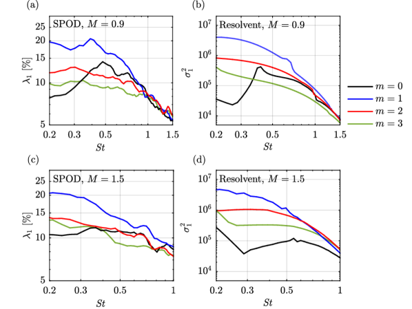
Figure 17: SPOD energy spectra (a,c) and optimal resolvent gains (b,d) as in figure 10, but for the transsonic (a,b) and the supersonic (c,d) jet.

Figure 17 shows the leading SPOD mode energy and the optimal resolvent gain for the transsonic (top) and supersonic (bottom) cases. As in figure 10, spectra for the first four azimuthal wavenumbers are reported. Like in the subsonic case, favorable agreement of the qualitative trends is found between the SPOD analysis and the resolvent model. The presence of the acoustic resonance mechanism associated with the trapped modes is apparent in the gains. The peaks seen in figure 10(a), for example at $(\mbox{{St}},m)\approx(0.4,0)$ and $(\mbox{{St}},m)\approx(0.7,1)$, coincide with the frequencies of branches of trapped acoustic modes. The associated eigenvalues are only marginally damped in the global spectra of the same operator (Schmidt et al., 2017). This proximity of the eigenvalues to the real axis explains the peaks in the gain curves as a pseudo-resonance. The acoustic branch locations are marked in the resolvent gain spectra shown in figure 19 (appendix A).

7 Summary and conclusions

Large-scale structures taking the form of spatially modulated wavepackets have long been observed in turbulent jets and past attempts to model them using linear theory have met partial success (Jordan & Colonius, 2013). In this paper, we use SPOD to distill these wavepackets from a high-fidelity numerical simulation and demonstrate that a resolvent mean flow model predicts them in great detail. Both approaches paint a consistent picture of two coexisting mechanisms. The KH-type instability is active, over a range of frequencies and azimuthal wavenumbers, in the initial shear-layer whereas the region downstream of the close of the potential core is dominated by Orr-type waves. Moreover, in the initial shear layer region, Orr-type waves are also present but not readily observed as they are swamped by the high-gain KH waves. We quantified both types of structures over a range of frequencies and azimuthal wavenumbers. In addition to their differing spatial regions of dominance, they are distinguished by their spatial support, phase speed and frequency scaling. KH-type wavepackets can be regarded as local spatial instabilities. They convect with a phase velocity of $c_{ph}\approx 0.8U_{j}$ and are triggered by fluctuations close to the nozzle. This spatial separation between optimal forcing and response characterizes a convective non-normality (Marquet et al., 2009) in the presence of a spatial instability mechanism (Alizard et al., 2009; Dergham et al., 2013; Beneddine et al., 2016). By contrast, Orr-type waves convect at a lower speed in accordance with the jet’s velocity-decay rate, and are most effectively sustained by distributed forcing. Both the KH and Orr waves peak at the hight of the critical layer in the radial directions and are optimally forced by the Orr-mechanism.

In the LES data analysis, frequencies at which the KH-mechanism dominates are identified by a separation between the first and second eigenvalues in the SPOD spectrum, and the resolvent gain reliably predicts this low-rank behavior. Although this low-rank behavior can in principal be inferred from the success of past studies based on spatial linear stability theory (e.g. Michalke, 1971), it is most compellingly revealed in the SPOD and resolvent spectra. Equally important to its presence is its absence. For $m=0$ at very low frequencies, for example, the KH-mechanism is absent as the initial shear-layer becomes short as compared to the perturbation wavelength. Here, the jet exhibits non-low-rank behavior and both the SPOD and the resolvent model predict the coexistence of Orr-type waves of similar energy. For $m=1$, on the contrary, the KH-mechanism persists to very low frequencies.

The non-low-rank behavior explains why wavepacket models based on PSE such as the ones by Gudmundsson & Colonius (2011), Cavalieri et al. (2013) and Sinha et al. (2014) fail at these the very low frequencies for $m=0$. For example, the PSE method is initialized with the locally most unstable spatial wave, which is then propagated downstream by space-marching. In the non-low-rank regime, this mode does not optimally trigger transient growth and appears as a sub-dominant resolvent mode. Furthermore, as volumetric forcing by the turbulence is not accounted for, PSE cannot support the dominant Orr-type waves. With the goal in mind to further improve its predictive capabilities, in particular at low frequencies, we plan to model the second-order statistics of the forcing and incorporate them into a resolvent-based jet noise model in future work.

Appendix

Appendix A Spectral analysis and resolvent model for the transonic and supersonic jets

This appendix reports the additional results for the SPOD and resolvent analyses of the $M=0.9$ and $M=1.5$ jets, that were omitted in §6 for brevity. The resolvent gain spectra for the transonic and supersonic jets are reported in figures 19 and 21, and the SPOD energy spectra in figures 18 and 20, respectively. The azimuthal wavenumber dependence of the optimal gain and SPOD energy is studied in figure 22 for both jet configurations.

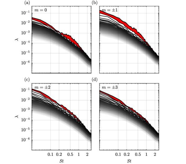
Figure 18: SPOD eigenvalue spectra ($\blacksquare\!{\color[rgb]{0.5,0.5,0.5}\blacksquare}\!\square$, $\lambda_{1}\!>\!\lambda_{2}\!>\!\cdots\!>\!\lambda_{N}$) as in figure 3, but for the $M=0.9$ transsonic jet: (a) $m=0$; (b) $m=1$; (c) $m=2$; (d) $m=3$.

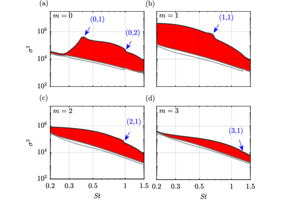
Figure 19: Optimal energetic gain spectra ( , $\sigma_{1-3}$) as in figure 8 but for the transonic $M=0.9$ jet: (a) $m=0$; (b) $m=1$; (c) $m=2$; (d) $m=3$. The locations of the branches of trapped acoustic modes are indicated by the doublets $(m,n_{r})$, where $n_{r}$ is their radial order and $m$ the azimuthal wavenumber, as before. See (Towne et al., 2017b; Schmidt et al., 2017) for details.

In figure 19, the locations of the branches of trapped acoustic modes (Schmidt et al., 2017) are indicated, and their effect on the resolvent gain becomes apparent.

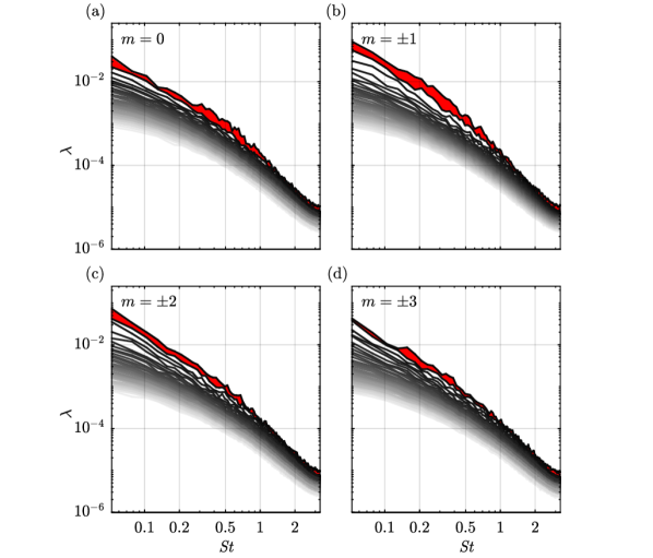
Figure 20: SPOD eigenvalue spectra ($\blacksquare\!{\color[rgb]{0.5,0.5,0.5}\blacksquare}\!\square$, $\lambda_{1}\!>\!\lambda_{2}\!>\!\cdots\!>\!\lambda_{N}$) as in figure 3, but for the $M=1.5$ supersonic jet: (a) $m=0$; (b) $m=1$; (c) $m=2$; (d) $m=3$.

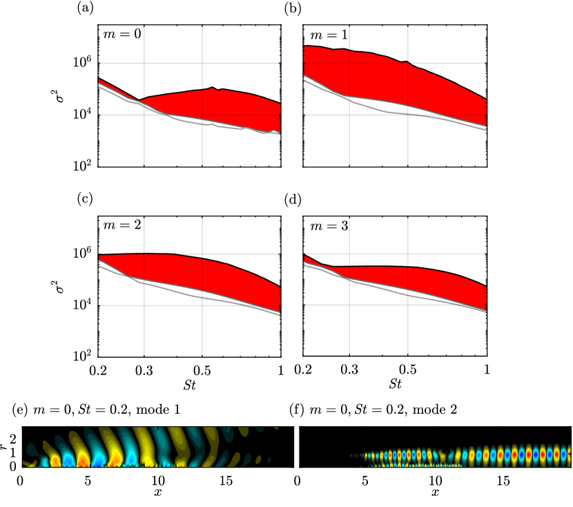
Figure 21: Optimal energetic gain spectra ( , $\sigma_{1-3}$) as in figure 8 but for the supersonic $M=1.5$ jet: (a) $m=0$; (b) $m=1$; (c) $m=2$; (d) $m=3$. The pressure of the leading and first suboptimal modes at $(m,\mbox{{St}})=(0,0.2)$ are shown in (e) and (f), respectively.

For the supersonic jet shown in figure 21, a sudden change of slope is observed in the suboptimal gain curves. An inspection of the modal structures confirms that this change is associated with the presence of upstream-propagating subsonic waves (Tam & Hu, 1989), as previously discussed in the context of figure 16. In panels 21(e,f), the dominant and the first suboptimal mode for $(m,\mbox{{St}})=(0,0.2)$ are compared. At this frequency, the leading mode is of KH-type, whereas the second mode is of mixed Orr/acoustic type. In the second mode in panel 21(f), the acoustic wave component appears isolated in the stretch $6\lesssim x\lesssim 12$ along the axis. The trapped acoustic waves in the transonic jet and the upstream-propagating subsonic waves in the supersonic jet have a direct effect on the resolvent gain, as can be seen in figures 19 and 21, respectively. It is a remarkable property of the resolvent analysis that it is able to isolate these physical phenomena. Both types of waves are also apparent in the SPOD modes. However, they appear much less pronounces in the latter. This discrepancy is also reflected in the SPOD energy spectra in figures 18(a) and 20(b), respectively. In the SPOD spectra, the effect of these special waves is not apparent. This observation further highlights the importance of the second-order forcing statistics. Other factors are the Reynolds number dependance and the choice of norm.

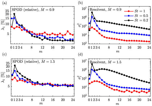
Figure 22: Azimuthal wavenumber dependence of the relative modal energy of the SPOD (a,c), and the optimal resolvent gains (b,d) as in figure 15, but for the transsonic (a,b), and supersonic jet (c,d).

References

- Alizard et al. (2009) Alizard, F., Cherubini, S. & Robinet, J.-C. 2009 Sensitivity and optimal forcing response in separated boundary layer flows. Physics of Fluids 21.
- Arndt et al. (1997) Arndt, R. E. A., Long, D. F. & Glauser, M. N. 1997 The proper orthogonal decomposition of pressure fluctuations surrounding a turbulent jet. Journal of Fluid Mechanics 340, 1–33.
- Aubry (1991) Aubry, N. 1991 On the hidden beauty of the proper orthogonal decomposition. Theoretical and Computational Fluid Dynamics 2 (5), 339–352.
- Beneddine et al. (2016) Beneddine, S., Sipp, D., Arnault, A., Dandois, J. & Lesshafft, L. 2016 Conditions for validity of mean flow stability analysis. Journal of Fluid Mechanics 798, 485–504.
- Bishop et al. (1971) Bishop, K. A., Ffowcs Williams, J. E. & Smith, W. 1971 On the noise sources of the unsuppressed high-speed jet. Journal of Fluid Mechanics 50 (1), 21–31.
- Brès et al. (2017a) Brès, G., Jordan, P., Le Rallic, M., Jaunet, V., Cavalieri, A. V. G, Towne, A., Lele, S., Colonius, T. & Schmidt, O. T. 2017a Importance of the nozzle-exit boundary-layer state in subsonic turbulent jets. submitted to Journal of Fluid Mechanics .
- Brès et al. (2017b) Brès, G. A., Ham, F. E., Nichols, J. W. & Lele, S. K. 2017b Unstructured large-eddy simulations of supersonic jets. AIAA Journal 55 (4), 1164–1184.
- Cavalieri et al. (2011) Cavalieri, A. V. G., Jordan, P., Agarwal, A. & Gervais, Y. 2011 Jittering wave-packet models for subsonic jet noise. Journal of Sound and Vibration 330 (18), 4474–4492.
- Cavalieri et al. (2013) Cavalieri, A. V. G, Rodríguez, D., Jordan, P., Colonius, T. & Gervais, Y. 2013 Wavepackets in the velocity field of turbulent jets. Journal of Fluid Mechanics 730, 559–592.
- Cavalieri et al. (2016) Cavalieri, A. V. G., Sasaki, K., Jordan, P., Schmidt, O. T., Colonius, T. & Br s, G. A. 2016 High-frequency wavepackets in turbulent jets. In 22nd AIAA/CEAS Aeroacoustics Conference. American Institute of Aeronautics and Astronautics (AIAA).
- Chu (1965) Chu, B.-T. 1965 On the energy transfer to small disturbances in fluid flow (Part I). Acta Mechanica 1 (3), 215–234.
- Citriniti & George (2000) Citriniti, J. H. & George, W. K. 2000 Reconstruction of the global velocity field in the axisymmetric mixing layer utilizing the proper orthogonal decomposition. Journal of Fluid Mechanics 418, 137–166.
- Crighton & Gaster (1976) Crighton, D. G. & Gaster, M. 1976 Stability of slowly diverging jet flow. Journal of Fluid Mechanics 77 (02), 397–413.
- Crighton & Huerre (1990) Crighton, D. G. & Huerre, P. 1990 Shear-layer pressure fluctuations and superdirective acoustic sources. Journal of Fluid Mechanics 220, 355–368.
- Crow & Champagne (1971) Crow, S. C. & Champagne, F. H. 1971 Orderly structure in jet turbulence. Journal of Fluid Mechanics 48 (03), 547–591.
- Dergham et al. (2013) Dergham, G., Sipp, D. & Robinet, J-C. 2013 Stochastic dynamics and model reduction of amplifier flows: the backward facing step flow. Journal of Fluid Mechanics 719, 406–430.
- Farrell & Ioannou (1993) Farrell, B. F. & Ioannou, P. J. 1993 Stochastic forcing of the linearized navier–stokes equations. Physics of Fluids A: Fluid Dynamics (1989-1993) 5 (11), 2600–2609.
- Garnaud et al. (2013) Garnaud, X., Lesshafft, L., Schmid, P. J. & Huerre, P. 2013 The preferred mode of incompressible jets: linear frequency response analysis. Journal of Fluid Mechanics 716, 189–202.
- Glauser et al. (1987) Glauser, M. N., Leib, S. J. & George, W. K. 1987 Coherent structures in the axisymmetric turbulent jet mixing layer. Turbulent shear flows 5, 134–145.
- Gudmundsson & Colonius (2011) Gudmundsson, K. & Colonius, T. 2011 Instability wave models for the near-field fluctuations of turbulent jets. Journal of Fluid Mechanics 689, 97–128.
- Jeun et al. (2016) Jeun, J., Nichols, J. W. & Jovanović, M. R. 2016 Input-output analysis of high-speed axisymmetric isothermal jet noise. Physics of Fluids (1994-present) 28 (4), 047101.
- Jordan & Colonius (2013) Jordan, P. & Colonius, T. 2013 Wave packets and turbulent jet noise. Annual Review of Fluid Mechanics 45, 173–195.
- Jordan et al. (2017) Jordan, P., Zhang, M., Lehnasch, G. & Cavalieri, A. V. G. 2017 Modal and non-modal linear wavepacket dynamics in turbulent jets. In 23rd AIAA/CEAS Aeroacoustics Conference, p. 3379.
- Jovanović & Bamieh (2005) Jovanović, M. R. & Bamieh, B. 2005 Componentwise energy amplification in channel flows. Journal of Fluid Mechanics 534, 145–183.
- Lumley (1967) Lumley, J. L. 1967 The structure of inhomogeneous turbulent flows. In Atmospheric turbulence and radio propagation (ed. A. M. Yaglom & V. I. Tatarski), pp. 166–178. Moscow: Nauka.
- Lumley (1970) Lumley, J. L. 1970 Stochastic tools in turbulence. New York: Academic Press.
- Marquet et al. (2009) Marquet, O., Lombardi, M., Chomaz, J.-M., Sipp, D. & Jacquin, L. 2009 Direct and adjoint global modes of a recirculation bubble: lift-up and convective non-normalities. Journal of Fluid Mechanics 622, 1–21.
- McKeon & Sharma (2010) McKeon, B. J. & Sharma, A. S. 2010 A critical-layer framework for turbulent pipe flow. Journal of Fluid Mechanics 658, 336–382.
- Mettot et al. (2014) Mettot, C., Sipp, D. & Bézard, H. 2014 Quasi-laminar stability and sensitivity analyses for turbulent flows: Prediction of low-frequency unsteadiness and passive control. Physics of Fluids (1994-present) 26 (4), 045112.
- Michalke (1971) Michalke, A. 1971 Instability of a compressible circular free jet with consideration of the influence of the jet boundary layer thickness. Z. für Flugwissenschaften 19 (8), 319–328.
- Moarref & Jovanović (2012) Moarref, R. & Jovanović, M. R. 2012 Model-based design of transverse wall oscillations for turbulent drag reduction. Journal of Fluid Mechanics 707, 205–240.
- Monokrousos et al. (2010) Monokrousos, A., Åkervik, E., Brandt, L. & Henningson, D. S. 2010 Global three-dimensional optimal disturbances in the blasius boundary-layer flow using time-steppers. Journal of Fluid Mechanics 650, 181–214.
- Moore (1977) Moore, C. J. 1977 The role of shear-layer instability waves in jet exhaust noise. Journal of Fluid Mechanics 80 (02), 321–367.
- Pope (2000) Pope, S. B. 2000 Turbulent Flows, 1st edn. Cambridge University Press.
- Reddy & Henningson (1993) Reddy, S. C. & Henningson, D. S. 1993 Energy growth in viscous channel flows. Journal of Fluid Mechanics 252 (1), 209–238.
- Reddy et al. (1993) Reddy, S. C., Schmid, P. J. & Henningson, D. S. 1993 Pseudospectra of the Orr-Sommerfeld operator. SIAM Journal on Applied Mathematics 53 (1), 15–47.
- Sasaki et al. (2017) Sasaki, K., Cavalieri, A. V. G., Jordan, P., Schmidt, O. T., Colonius, T. & Brès, G. A. 2017 High-frequency wavepackets in turbulent jets. Journal of Fluid Mechanics 830, R2.
- Schlinker et al. (2009) Schlinker, R. H., Simonich, J. C., Shannon, D. W., Reba, R. A., Colonius, T., Gudmundsson, K. & Ladeinde, F. 2009 Supersonic jet noise from round and chevron nozzles: experimental studies. AIAA paper 3257, 2009.
- Schmid & Henningson (2001) Schmid, P.J. & Henningson, D. S. 2001 Stability and Transition in Shear Flows, 1st edn. Springer-Verlag New York.
- Schmid (2010) Schmid, P. J. 2010 Dynamic mode decomposition of numerical and experimental data. Journal of Fluid Mechanics 656, 5–28.
- Schmidt et al. (2017) Schmidt, O. T., Towne, A., Colonius, T., Cavalieri, A. V. G., Jordan, P. & Brès, G. A. 2017 Wavepackets and trapped acoustic modes in a turbulent jet: coherent structure eduction and global stability. Journal of Fluid Mechanics 825, 1153–1181.
- Semeraro et al. (2016) Semeraro, O., Lesshafft, L., Jaunet, V. & Jordan, P. 2016 Modeling of coherent structures in a turbulent jet as global linear instability wavepackets: Theory and experiment. International Journal of Heat and Fluid Flow 62, 24–32.
- Sinha et al. (2014) Sinha, A., Rodríguez, D., Brès, G. A. & Colonius, T. 2014 Wavepacket models for supersonic jet noise. Journal of Fluid Mechanics 742, 71–95.
- Sipp & Marquet (2013) Sipp, D. & Marquet, O. 2013 Characterization of noise amplifiers with global singular modes: the case of the leading-edge flat-plate boundary layer. Theoretical and Computational Fluid Dynamics 27 (5), 617–635.
- Sirovich (1987) Sirovich, L. 1987 Turbulence and the dynamics of coherent structures. Quarterly of applied mathematics 45 (3), 561–571.
- Suzuki & Colonius (2006) Suzuki, T. & Colonius, T. 2006 Instability waves in a subsonic round jet detected using a near-field phased microphone array. Journal of Fluid Mechanics 565 (1), 197–226.
- Tam & Hu (1989) Tam, C. K. W. & Hu, F. Q. 1989 On the three families of instability waves of high-speed jets. Journal of Fluid Mechanics 201, 447–483.
- Tissot et al. (2017) Tissot, G., Zhang, M., Lajús, F. C., Cavalieri, A. V. G. & Jordan, P. 2017 Sensitivity of wavepackets in jets to nonlinear effects: the role of the critical layer. Journal of Fluid Mechanics 811, 95–137.
- Towne et al. (2017a) Towne, A., Brès, G. A. & Lele, S. K. 2017a A statistical jet-noise model based on the resolvent framework. AIAA Paper 2017-3406 .
- Towne et al. (2017b) Towne, A., Cavalieri, A. V. G., Jordan, P., Colonius, T., Schmidt, O. T., Jaunet, V. & Brès, G. A. 2017b Acoustic resonance in the potential core of subsonic jets. Journal of Fluid Mechanics 825, 1113–1152.
- Towne et al. (2015) Towne, A., Colonius, T., Jordan, P., Cavalieri A. V. G. & Brès, G. A. 2015 Stochastic and nonlinear forcing of wavepackets in a mach 0.9 jet. In 21st AIAA/CEAS Aeroacoustics Conference, p. 2217.
- Towne et al. (2017c) Towne, A., Schmidt, O. T. & Colonius, T. 2017c Spectral proper orthogonal decomposition and its relationship to dynamic mode decomposition and resolvent analysis. arXiv preprint arXiv:1708.04393 .
- Trefethen et al. (1993) Trefethen, L. N., Trefethen, A. E., Reddy, S. C. & Driscoll, T. A. 1993 Hydrodynamic stability without eigenvalues. Science 261 (5121), 578–584.
- Zare et al. (2017) Zare, A., Jovanović, M. R. & Georgiou, T. T. 2017 Colour of turbulence. Journal of Fluid Mechanics 812, 636–680.