Local Density of the Bose Glass Phase

Abstract

We study the Bose-Hubbard model in the presence of on-site disorder in the canonical ensemble and conclude that the local density of the Bose glass phase behaves differently at incommensurate filling than it does at commensurate one. Scaling of the superfluid density at incommensurate filling of $\rho=1.1$ and on-site interaction $U=80t$ predicts a superfluid-Bose glass transition at disorder strength of $\Delta_{c}\approx 30t$. At this filling the local density distribution shows skew behavior with increasing disorder strength. Multifractal analysis also suggests a multifractal behavior resembling that of the Anderson localization. Percolation analysis points to a phase transition of percolating non-integer filled sites around the same value of disorder. Our findings support the scenario of percolating superfluid clusters enhancing Anderson localization near the superfluid-Bose glass transition. On the other hand, the behavior of the commensurate filled system is rather different. Close to the tip of the Mott lobe ($\rho=1,U=22t$) we find a Mott insulator-Bose glass transition at disorder strength of $\Delta_{c}\approx 16t$. An analysis of the local density distribution shows Gaussian like behavior for a wide range of disorders above and below the transition. The behaviors of the superfluid-Bose glass transition call for a thorough finite size scaling analysis of percolation and multifractality to understand the universality of the transition.

I Introduction

The Bose-Hubbard model Gersch was originally proposed to demonstrate the existence of a macroscopically occupied state under a repulsive interaction. By introducing quenched disorder Gimarchi ; Fisher this model exhibits a complex phase diagram. Many theoretical investigations of disordered interacting bosonic models followed DFisher ; Fisher ; Freericks ; Scalettar ; Krauth ; Kisker ; Kisker2 ; Carusotto ; Amico ; Semerjian ; Anders ; Rancon ; Yokoyama ; Pai ; Dawson ; Lacki ; Hettiarachchilage ; Zhang ; Sheshadri ; Priyadarshee ; Gurarie ; Yao ; Meier ; Soyler ; Zuniga ; Thomson ; Ng ; Hitchcock ; Singh ; Oosten ; Capogrosso-Sansone ; Lin ; Niederle ; Batrouni ; Hu ; Pollet early experiments on ⁴He films absorbed on porous media Finotello ; Angolet ; Bishop ; Crowell ; Csathy . More recently, due to advances on optical lattice experiments, the Bose-Hubbard model has also become relevant in the reign of atomic physics Jaksch ; Bloch ; Greiner . Indeed, it quickly becomes the most important venue for the physical realization of the Bose-Hubbard model Greiner .

In the absence of disorder the Bose-Hubbard model is rather well understood, but the physics of the disordered model has shown to be much complicated. An outstanding controversial issue is related to the quantum phase transition at commensurate filling. Early studies suggested that a direct superfluid Mott insulator transition was unlikely though not fundamentally impossibleFisher . A third phase, the compressible and gapless Bose glass, intervenes between the superfluid and Mott insulator. Recent arguments justified the existence of the Bose glass upon the destruction of the Mott insulator based on the appearance of rare but compressible superfluid clusters Pollet ; Griffiths ; Gurarie . Observation of a superfluid-Bose glass transition has been reported in recent cold atoms experimentsPasienski .

While the phase diagram of the disordered Bose-Hubbard model has been extensively studied, the nature of the Bose glass has not received that much attention. A real space renormalization group study has claimed that the local density is not self averaging for the Bose glass phase Hegg . It has further been proposed that replica symmetry is broken at higher than two dimensions Thomson . There are reports which suggest that the Bose glass phase can be understood as a system of non-percolating superfluid clusters Niederle . But, a recent Quantum Monte Carlo study on the related hard core Bose model suggests that the transition is not due to percolationPablo .

A simple physical interpretation of the Bose glass phase, borrowed from Anderson localization, is that the virtually free bosons in the presence of a sufficiently strong disorder potential localize Weichman . The wavefunction of the Anderson model has been studied in great detail in recent years Rodriguez ; Ujfalusi ; Castellani ; Wegner1979 ; Wegner1980 ; Yakubo ; Lindinger . A prominent feature of the localized phase is the skew distribution of its local density Schubert . More interestingly, around the critical point between the metallic and the localized phase the wavefunction exhibits multifractal behavior Rodriguez ; Ujfalusi ; Moore . If the Bose glass can be interpreted as an Anderson localized phase, a natural question is whether some of those behaviors can be rediscovered in the Bose-Hubbard model.

In this paper, we focus on the nature of the Bose glass and its transition to the superfluid phase. In particular, we investigate the behavior of the local density distribution at a commensurate, $\rho=1$, and an incommensurate filling, $\rho=1.1$. We find the local density distribution broadens as the disorder increases, but there are substantial difference between the systems at and away from the commensurate filling. We perform multifractal and percolation analyses and find rather strong evidences that multifractal behavior exists near the Bose glass superfluid transition, where the percolation clusters formed by the non-integer filled sites can also be observed.

The paper is organized as follows. In Section II we introduce the model and the parameters for our study. In Section III we discuss the effects of disorder on the incommensurate superfluid phase. In Section IV we present the effect of disorder on the commensurate Mott phase and highlight the difference in the local density distribution for the two fillings. We conclude in Section V. In the Appendix, we provide additional details of the percolation analysis.

II Model

The Hamiltonian for the disorder Bose-Hubbard model on a two-dimensional square lattice takes the form:

$$\hat{\mathcal{H}} = -t\sum_{\langle i,j\rangle}\Big{(}a_{i}^{\dagger}a_{j}^{\phantom{\dagger}}+H.c.\Big{)}$$ (1)

$$+\frac{U}{2}\sum_{i}\hat{n}_{i}\Big{(}\hat{n}_{i}-1\Big{)}+{\Delta\sum_{i}\epsilon_{i}\hat{n}_{i}},$$

where $a_{i}^{\dagger}$ ($a_{i}$) is the creation (annihilation) operator of a soft-core boson at lattice site $i$ with number operator $n_{i}=a_{i}^{\dagger}a_{i}^{\phantom{\dagger}}$. The sum $\sum\limits_{\langle i,j\rangle}$ runs over all distinct pairs of first neighboring sites $i$ and $j$, $t=1$ is the hopping integral between neighboring sites, $U$ is the strength of the on-site interaction, $\epsilon_{i}$ is a uniformly distributed random variable in the interval $[-\frac{1}{2},+\frac{1}{2}[$, and $\Delta$ is the disorder strength. The inverse temperature is set at $\beta=L$ unless otherwise stated.

We perform a quantum Monte Carlo study of this model within the canonical ensemble using the Stochastic Green Function algorithm SGF ; DirectedSGF with global space-time updates SpaceTime . As only a rather small system size (256 lattice sites) can be studied, the choice of ensemble may affect the data. As we are particularly interested in the differences between commensurate and incommensurate fillings, we use the canonical ensemble in which the number of particles is fixed during the entire sampling process. Unlike most of the Quantum Monte Carlo methods the Stochastic Green Function algorithm allows to set the canonical ensemble rather easily SGF ; DirectedSGF ; SpaceTime .

III Introducing Disorder into the Superfluid Phase

We consider a system with incommensurate filling factor or average density $\rho=1.1$, which in the absence of disorder shows superfluid behavior. Then, we introduce disorder and identify the critical point of the transition to a disordered phase. Our choice of the value $\rho=1.1$ does not have any intrinsic physical meaning. We expect similar results for other values close-by. However, we do not attempt to choose a value too close to $\rho=1$ due to the anticipated difficulties to locate the superfluid-Bose glass transition point numerically.

III.1 Superfluid Density

We follow the standard procedure to detect a transition between superfluid and non-superfluid phases by monitoring the superfluid density, $\rho_{s}$. The Hamiltonian (1) satisfies the conditions needed for using the conventional formula which relates the winding number to the superfluid density  Superfluid . Then, the superfluid density, $\rho_{s}$, can be calculated via the winding number, $W$, as $\displaystyle\rho_{s}=\frac{\langle W^{2}\rangle}{4t\beta}$ where $\beta$ is the inverse temperature Pollock .

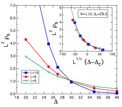
Figure 1: (Color online) $L^{2}\rho_{s}$ versus disorder strength, $\Delta$, for different system sizes ($L=6,8,16$), density $\rho=1.1$, and on-site interaction $U=80t$. The scaling analysis shows that the three curves cross at the critical disorder strength, $\Delta_{c}\approx 30t$. The data points are based on averaging the data from simulations of 1,000 disorder realizations.

Fig. 1 displays $\rho_{s}L^{2}$ as a function of disorder strength $\Delta$ for three different system sizes: $L=6,8,$ and $16$. In the neighborhood of the critical disorder strength $\Delta_{c}$, the superfluid density follows the scaling ansatz $\rho_{s}\sim L^{-z}g(L^{\frac{1}{\nu}}(\Delta-\Delta_{c}))$, where $z$ is the dynamical critical exponent, $\nu$ the correlation length exponent, and $g(...)$ a universal scaling function Wang . We based our finite size scaling on the assumption that $z=2$, the spatial dimension Fisher . We locate the critical disorder at $\Delta_{c}=29.5t$ and the correlation length exponent $\nu=1.15$.

Our intent is not to pinpoint the critical point and its associated exponents with a very high precision, but to roughly locate the critical disorder and analyze the local density distribution for disorder strength close to the critical value. High precision calculations of the critical exponents of related models have been attempted in recent studies Ng ; Meier ; Pablo ; Wang . For a more precise analysis one has to consider the scaling correction, and the goodness of fit, which could be rather challenging for the Bose-Hubbard model Ng ; Pablo ; Ujfalusi ; Rodriguez ; Moore ; Wang . We note that the value of $\nu=1.15$ we obtain is close to the latest estimates Ng ; Pablo ; Meier .

III.2 Local Density Distribution

After we established the critical strength from scaling the superfluid density, we focus on the local density. Fig. 2 displays local density histograms for system size $L=16$, density $\rho=1.1$, interaction $U=80t$ for several disorder strengths. Each calculation includes 1,000 disorder realizations. The inset shows the same quantities in a semi-logarithmic scale.

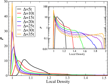
Figure 2: (Color online) Histograms of the probability, $P$, versus local density for system size $L=16$, density $\rho=1.1$, interaction $U=80t$, and disorder strength between $\Delta=5t$ and $\Delta=35t$. Each calculation includes 1,000 disorder realizations. The inset shows the same quantities in semi-log scale.

Fig. 2 shows that while the behavior of the local density distribution is close to Gaussian at small disorder, it is already visibly deviates from Gaussian at the $\Delta=5t$, it becomes skew with a typical value very close to $\rho=1$ and a long tail, cut off around 2.0, for large values of the disorder strength. For

The skewness and long tail of the density distribution is the hallmark of the localized phase in the single particle Anderson model MacKinnon ; Schubert ; Moore ; Anderson . However, a true long tail distribution with no upper bound does not exist in the present model, as the local density is always cutoff at integer filling, most probably due to the Hubbard energy penalty. We emphasize that the model we study is the standard Bose-Hubbard model without hardcore constraint. Therefore these finding suggest that even in the Bose glass phase the long tailed distribution does not extent all the way to infinity, but it is truncated due to the energy penalty for multiple occupation of a local site.

We corroborate these observations by calculating the skewness, kurtosis and mode of the local density distribution as function of disorder strength. These measurements quantify the broadening of the distribution as the disorder increases. Fig. 3 shows that both the skewness and kurtosis grow with disorder strength to reach an apparent plateau for large disorder values. The local density distribution for large disorder has kurtosis close to $8$ which is far from that the kurtosis of $3$ of a Gaussian. According to the typical medium theory for Anderson localization, the localized phase is signal by a typical local density equal to zero Ekuma ; Dobrosavljevic ; Janssen , we also plot the mode of the distributions in Fig. 3, bottom panel. We clearly see the mode of the distribution shifting from $1.1$ to $1$ as the disorder increases and settling at $1$ for disorder $\Delta$ larger than $20t$.

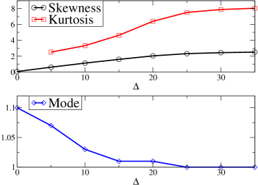
Figure 3: (Color online) The skewness and kurtosis (upper panel), and mode (lower panel) of the local density distribution as a function of disorder strength for system size $L=16$, density $\rho=1.1$, and interaction $U=80t$ as a function of disorder $\Delta$. The distribution for $\Delta=0$ is very narrow and its kurtosis cannot be calculated with enough precision. Mode is estimated from the histogram of the local density distribution with bin size $0.01$.

III.3 Multifractal Analysis

For $\rho=1.1$ the Bose glass can be considered as a diluted particles phase on a Mott insulating background where, in first approximation, the bosons exceeding integer occupation behave as independent particles in a random potential where each local site is already occupied by one particle. The quasiparticles in a two-dimensional random potential lattice localize unconditionally for the AI class Anderson ; MacKinnon ; Atland ; Evers . Since Figs. 2 and 3 support this point of view, we perform a multifractal analysis to look for similarities with the Anderson model Wegner1979 ; Wegner1980 ; Castellani ; Rodriguez ; Ujfalusi ; Moore .

The multifractal analysis is based on the basic idea that the moments of a distribution cannot be described by a single exponent, but they are a continuous function of the order of the moment. Calculations are performed by dividing the system into different box sizes and calculating the moment for each box size. The moment is defined as:

$$Z_{q}(l)=\sum_{i}^{N_{l}}(m_{i}(l))^{q},$$ (2)

where $m_{i}(l)$ is the local quantity (mass by convention) for the $i^{th}$ box, $N_{l}$ is the total number of boxes of linear size $l$, and $q$ is any real number. For our data with system size $L=16$, we choose $l=L/2,L/4$, and $L/8$. The multifractal dimension can be defined as the limit of the ratio of the logarithm of the moment to the logarithmic of the box size divide by $(q-1)$,

$$D_{q}=\frac{1}{q-1}\lim_{l\to 0}\frac{\log(Z_{q}(l))}{\log l}.$$ (3)

In practice, the limit of $l\to 0$ is estimated by linear extrapolation of $\log(Z_{q}(l))$ vs $\log l$.

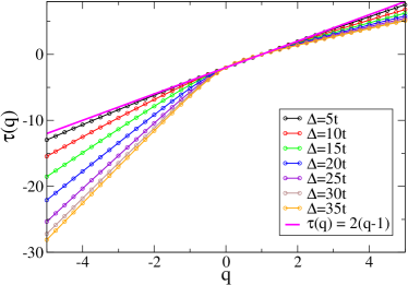
Figure 4: (Color online) Mass exponents of local density averaged over $1000$ disorder realizations. Local density measured for system size $L=16$, density $\rho=1.1$, and interaction $U=80t$ for disorder strengths $\Delta=5t,10t,15t,20t,25t,30t,$ and $35t$. The mass exponent of a non-fractal system is included ($\tau(q)=2(q-1)$) for comparison.

One can also define the mass exponent,

$$\tau(q)=(q-1)D_{q}.$$ (4)

There are two special points in the mass exponents: $q=1$ and $q=0$. For $q=1$, the mass exponent is always equal to zero provided that the input $m_{i}(L)$ is normalized. For $q=0$, the mass exponent is equal to the negative of the dimension of the support, in this case the support is a square lattice, therefore $\tau(q=0)=-2$. A multifractal distribution is defined as a distribution which possesses a nonlinear dependence between the mass exponent $\tau$ and the order of the moment $q$Nakayama ; Stanley ; Salat . For non-fractal systems, their mass exponent is simply given as $\tau(q)=2(q-1)$ for a system with support on a square lattice.

For the Bose-Hubbard model at incommensurate filling, we choose the mass as the deviation of the local density from an integer value: $m_{i}(L)=|\rho_{i}-1|$. This quantity is normalized for each disorder realization before performing the multifractal analysis. Then $\tau(q)$ is calculated for each realization separately, and averaged over 1,000 realizations for each disorder strength, $\Delta$. Three different box sizes are used, $l=8,4$ and $2$, and $41$ different moments between $q=-5$ and $q=5$. We use the package mfSBA for the analysis Saravia_2012 ; Saravia_2014 . Fig. 4 displays the mass exponent for different disorder strengths between $5t$ and $35t$. For system which does not exhibit multifractality, the mass exponent is a linear function, $\tau(q)=2(q-1)$, also included in Fig. 4. Note that for small values of the disorder $\tau(q)$ is very close to the non-fractal limit. As the disorder increases the $\tau(q)$ curves bend further from the straight line, in particular for negative values of the moment. This is a typical signal of multifractality Chhabra ; Halsey .

Another common measure of multifractality is the singularity spectrum $f(\alpha)$. For each value of $q$, we can define the Hausdorff dimension as

$$f(q)=\lim_{l\to 0}\frac{1}{\log\ell}\sum_{i}^{N_{l}}M_{i}(l,q)\log M_{i}(l,q),$$ (5)

where $M_{i}(l,q)=(m_{i}(l))^{q}/\sum_{j}^{N_{l}}(m_{j}(l))^{q}$. Similarly, for each value of $q$, we can define the average value of the singularity (distribution) strength as

$$\alpha(q)=\lim_{l\to 0}\frac{1}{\log\ell}\sum_{i}^{N_{l}}M_{i}(l,q)\log m_{i}(l).$$ (6)

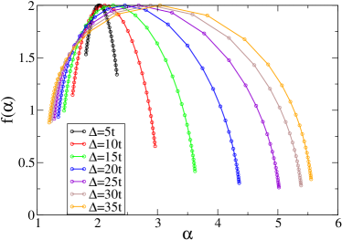
Figure 5: (Color online) Singularity spectrum of the local density averaged over 1000 disorder realizations. Local density measured for system size $L=16$, density $\rho=1.1$, and interaction $U=80t$ for the disorder strength values of $\Delta=5t,10t,15t,20t,25t,30t,$ and $35t$.

The above equations set up an implicit relation between $f$ and $\alpha$ Chhabra ; Halsey . For systems which are non-fractal, the singularity spectrum is concentrated around the point $(d,d)$, where $d$ is the system dimensionality, $d=2$ in our case. On the contrary, for monofractal or multifractal systems, an inverted curve with maximum at $(\alpha(q=0),f(q=0))$ is obtained, where $f(q=0)$ is the Hausdorff dimension of the support. Therefore for a square lattice $f(q=0)=2$ Halsey . The width of the singularity spectrum is a measure of the degree of multifractality. A monofractal distribution has a very narrow spectrum while a strongly multifractal quantity displays a wide singularity spectrum.

To calculate $f(\alpha)$ we use the same set of $q$ values we employ in the calculation of $\tau(q)$. Fig. 5 displays $f(\alpha)$ for several disorder strengths. For weak disorder within the superfluid phase the singularity spectrum shows a rather sharp peak close to $(2,2)$. As the disorder increases $\alpha(q=0)$ increases from around 2 to a value close to 3 for the largest disorder we explore. At the same time the singularity spectrum widens with increasing disorder.

We quantify the width of the distribution by fitting $f(\alpha)$ and then solving for the two solutions when $f(\alpha)=0$ to obtain $\alpha_{min}$ and $\alpha_{max}$. The width of the singularity spectrum can be defined as $W=\alpha_{max}-\alpha_{min}$ Stosic ; Zhao . Fig. 6 displays $W$ as an increasing function of the disorder strength. This widening increases faster between $\Delta=10t$ and $\Delta=25t$. For $\Delta>25t$ the width of the spectrum still increases but at a smaller rate.

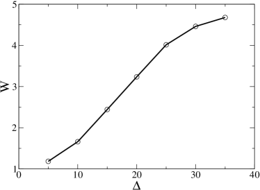
Figure 6: (Color online) Width ($W=\alpha_{max}-\alpha_{min}$) of the singularity spectrum of the local density averaged over 1000 disorder realizations for $L=16$, $\rho=1.1$, and $U=80t$.

Notice that the discussion and data presented in this section are not a multifractal finite size scaling analysis as has been done recently for the non-interacting models which possess Anderson localization transition Rodriguez ; Ujfalusi ; Moore ; Lindinger . The $\tau$, $\alpha$, and $f$ are estimated by using Eq. (2) to (6) for a system of size $L=16$. The notion of multifractality describes a system with scale invariant fluctuations which cannot be reduced to a single exponent. In general, scale invariance exists only at a second order transition point, which presumably is the superfluid-Bose glass transition within our model. For this very reason, one should only expect multifractality at exactly the critical value of disorder. The present analysis does not verify the scale invariance and it cannot pinpoint the value of the critical disorder based on multifractal finite size scaling analysis. Our data for the mass exponents and the singularity spectrum provide good evidence of multifractal behavior but it is not a definite proof.

III.4 Percolation Analysis

Since the early studies of the disordered Bose-Hubbard model, percolation has been considered as a mechanism to understand the superfluid to Bose glass transition Gao ; Sheshadri_1995 ; Niederle ; DellAnna ; Buonsante ; Barman . However, there are some difficulties in using percolation as a criterion to identify the transition. First, the choice of the local physical quantity is important. In this study we focus on the local density, but it is not entirely clear whether it is unique or even a proper choice. Second, regardless the method, local mean field or quantum Monte Carlo, the precision of the measured local quantity is limited.

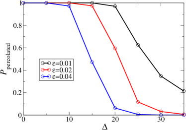
Figure 7: (Color online) The probability of finding a percolating cluster of non-integer filling. Three cutoffs for integer filling are shown, $\epsilon=0.01,0.02,$ and $0.04$ for the black, red, and blue lines, respectively. A local site is consider with integer occupation number if $|\rho_{i}-1|<\epsilon$. We define the probability of a percolating realization as $P_{\text{percolated}}=N_{\text{percolated}}/N$. $N_{\rm{percolated}}$ is the number of realizations with at least one percolated non-integer filling cluster. $N=1000$ independent realizations are used for each data point.

In our approach we need to choose a cutoff which discerns the sites with integer local occupation number from those with non-integer occupation. If a local site meets the criteria $|\rho_{i}-1|<\epsilon$, it is considered having an integer occupation number. The cutoff is clearly influenced by the precision of the measured quantity. We thus choose three different cutoffs, $\epsilon=0.01,0.02,$ and $0.04$; where $\epsilon=0.01$ is a realistic estimate for the smallest cutoff. We do not attempt to choose a smaller cutoff, as it would be too close to the Monte Carlo sampling error. Since, the local density is not an averaged quantity over the lattice, its measurement is generally more prone to carry a large statistical error. Fig. 7 shows the probability of a system with a non-integer percolating cluster as a function of disorder for these three different cutoffs. $P_{\rm percolated}=N_{\rm percolated}/N$, where $N_{\rm percolated}$ is the number of realizations with at least one percolated cluster of non-integer filled sites out of a total of $N$ realizations. See the appendix for the definition of percolation and examples of randomly chosen realizations for several values of disorder strength.

With the cutoff $\epsilon=0.01$, the probability of a percolating cluster becomes $50\%$ for $\Delta\simeq 27t$, which is slightly smaller than the critical disorder strength of $29.5t$ we found scaling the superfluid density. Most percolation transitions are second order, therefore one can attempt to perform a finite size scaling to locate the critical point and its exponents Kirkpatrick ; Shante . Given the available system sizes, we do not attempt to perform a more detail finite size scaling.

IV Introducing Disorder into the Mott-insulating Phase

In the absence of disorder the Bose-Hubbard model at integer fillings is well understood. For strong interaction the ground state is a Mott insulator. According to previous studies, the Bose glass phase can appear from very weak disorder Soyler . We note that a recent study suggests the Bose glass phase at weak disorder is anomalous Wang_MG . We are mostly interested in the local density distribution near the Mott insulator to a gapless Bose glass. As we did for the case of $\rho=1.1$ in the previous section, we first established the critical value of disorder at a fixed interaction. Since the tip of the Mott insulator lobe occurs at $U_{c}\approx 16.7t$ Soyler , we decide to introduce disorder at a slightly large value of $U=22t$.

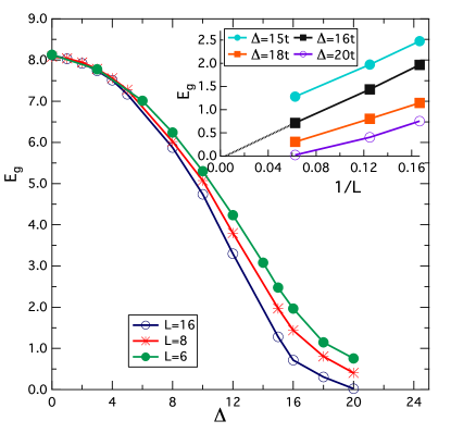
Figure 8: (Color online) Mott insulator gap $E_{g}$ versus disorder strength, $\Delta$, for different system sizes, $L=6,8,$ and $16$ at interaction $U=22t$. Data from $100$ disorder realizations are averaged for each data point. The inset displays $E_{g}$ for several values of $\Delta$ as a function of $1/L$. By extending those curves, we find $\Delta_{c}\approx 16t$. The corresponding inverse temperatures for the linear system sizes are $\beta t=12$ for $L=6$, $\beta t=16$ for $L=8$, and $\beta t=32$ for $L=16$. Data points are simulation results, lines are guides to the eye.

First, we look at the excitation gap. It has been suggested that there is no direct Mott insulator-superfluid transition Soyler ; Gurarie ; Pollet , thus the vanishing of the particle excitation gap corresponds to the Mott insulator-Bose glass transition. The Mott gap is calculated as follow. We obtain the chemical potential by adding a particle to the system as, $\mu_{1}=E(N+1)-E(N)$ and also by removing a particle from the system as $\mu_{2}=E(N)-E(N-1)$. The Mott gap is given as $E_{g}=\mu_{1}-\mu_{2}$. Fig. 8 displays the change of the energy gap, $E_{g}$, with increasing values of $\Delta$ for three different system sizes, $L=6,8,16$ at $U=22t$ for $100$ disorder realizations. Since we are dealing with finite systems we find a finite gap for each $\Delta$ we consider and we need to do a finite size scaling to infer the value of the gap. The inset in Fig. 8 shows $E_{g}$ as a function of $1/L$ for $\Delta=15t,16t,18t$ and $20t$. By extrapolating $E_{g}$ versus $1/L$ for different values of $\Delta$  we extract a value of the critical disorder of $\Delta_{c}\approx 15.7t$.

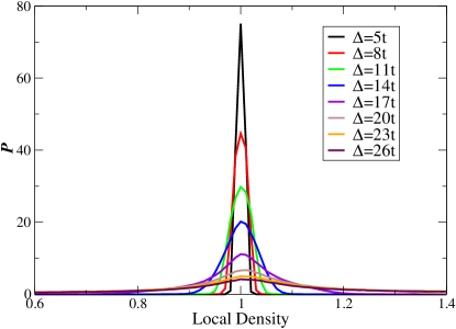
Figure 9: (Color online) Histograms of the probability, P, versus local density for disorder strength of $\Delta=5t,8t,11t,14t,17t,20t,23t$, and $26t$. The system size is $L=16$, the density is $\rho=1.0$, and the interaction is $U=22t$. $1600$ disorder realizations are calculated for each vale of disorder strength.

Fig. 9 displays the histogram of the local density for $1600$ disorder realizations, system size $L=16$, $\rho=1.0$, $\beta t=16$, and $U=22t$ for disorder strength, $\Delta$, between $5t$ and $26t$. The probability distribution of the local density for systems with weak disorder is Gaussian like; the distribution does spread out with increasing disorder but, unlike the $\rho=1.1$ case, its skewness is small and the local density spreads over both sides of the peak. This remains the case even for large values of disorder when the system is far from the Mott insulator phase ($\Delta_{c}\approx 15.7t$).

We further corroborate these observations by calculating the skewness, kurtosis, and mode of the distribution as a function of disorder. Fig. 10 shows those quantities and confirms our findings. Both the skewness and kurtosis are greatly reduced compared with the values for $\rho=1.1$. In particular the kurtosis, which can be interpreted as a measure of the density of outliers, is fairly close to $3$ even for rather strong disorder far away from the Mott insulator phase. In contrast with the case of $\rho=1.1$ the mode is fixed at a constant value $\sim 1$.

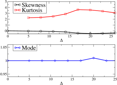
Figure 10: (Color online) The skewness and kurtosis (upper panel), and mode (lower panel) of the local density distribution as a function of disorder strength for system size $L=16$, density $\rho=1.0$, and interaction $U=22t$. The distribution for $\Delta=0$ is very narrow and its kurtosis cannot be calculated with enough precision. Mode is estimated from the histogram of the local density distribution with bin size $0.01$.

We conclude that for $\rho=1$ the validity of the analogy with Anderson localization is obscure since the picture of single particle in a disorder potential may not be valid. A many particle picture might be needed to explain the Bose glass phase at integer fillings.

V Conclusion

We study the spatial structure of the disordered Bose glass phase at both incommensurate and commensurate filling. We analyze our results at incommensurate filling based on a simple picture of the single particle Anderson localization. Given this picture, we test some of the characteristics of Anderson localization, such as the skewness of the distribution and multifractality. We find that for incommensurate filling ($\rho=1.1$), the local particle density has a skew distribution, and the multifractal analysis shows resemblance to that of the single particle Anderson localization. We also perform a percolation analysis to find that the probability of non-integer filling cluster does show a qualitative change near the transition between Bose glass and superfluid. The difficulty in precisely defining integer filling and the limitation in the available system size remain hindrances for a definite answer. If the transition is simply a standard classical percolation transition, then multifractality should not exist. A plausible scenario to reconcile multifractal and percolation behavior is that almost percolating clusters enhance Anderson localization. It is worthwhile to mention that the notion of percolation in the local superfluid amplitude, $\psi_{i}=<a_{i}>$, enhancing the superfluid to Bose glass transition due to localization has been proposed before Sheshadri_1995 . This picture does not preclude multifractality due to localization at the critical point. On the other hand, the commensurate ($\rho=1$) case shows very different behavior. The skewness and the moment of the local density distribution are greatly reduced when compared with the values obtained at incommensurate filling even when the system is far away from the Mott insulating phase. Clearly the local density distribution of the Bose glass at commensurate and incommensurate fillings cannot be described using the same picture. In particular, the single particle picture as that in the Anderson localization should fail.

VI Acknowledgment

This work was supported by NSF OISE-0952300 (KH, VGR and JM). Additional support was provided by the NSF EPSCoR Cooperative Agreement No. EPS-1003897 with additional support from the Louisiana Board of Regents (CM, KMT and MJ). Additional support (MJ) was provided by NSF Materials Theory grant DMR1728457. This work used the Extreme Science and Engineering Discovery Environment (XSEDE), which is supported by the National Science Foundation grant number ACI-1053575, and the high performance computational resources provided by the Louisiana Optical Network Initiative (http://www.loni.org).

*

Appendix A Patterns of Percolating Clusters

We discuss the percolation of non-integer filling clusters in Section III. In this appendix we randomly pick 32 realizations from four disorder strengths ($\Delta=15t,25t,30t,35t$) to illustrate the change of the number of percolating clusters as a function of disorder. The cutoff criteria for a local site with integer filling is defined as $|\rho_{i}-1|<\epsilon$. Figures below are for $\epsilon=0.01$. Each realization contains $16\times 16$ sites. The black and white squares represent sites with integer and non-integer occupation numbers, respectively. The blue area represents the cluster formed by the non-integer occupied sites. The cluster is defined starting at the top and contains all the sites with non-integer occupation which are connected. The realization is considered as percolated if there is one non-integer filling cluster which spans from the top to the bottom of the lattice. Since periodic boundary conditions are used in the calculation, this definition may underestimate the value of the disorder strength for the percolating cluster. For weak disorder, deep in the superfluid phase $\Delta=15t$, all the realizations are percolated. As the disorder increases, more and more realizations break into isolated fragments of non-integer filling sites.

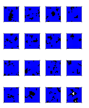
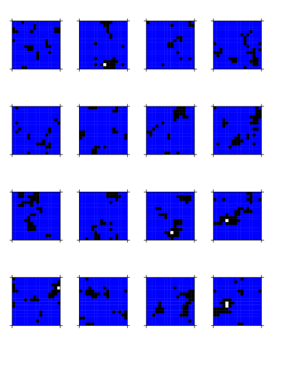
Figure 11: (Color online) Examples of the percolation pattern of local density for 32 different realizations with disorder strength $\Delta=15t$. All the clusters are percolated in this case. Clusters of size $L=16$, density $\rho=1.1$, and interaction $U=80t$.

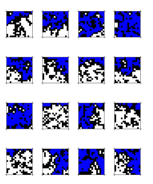
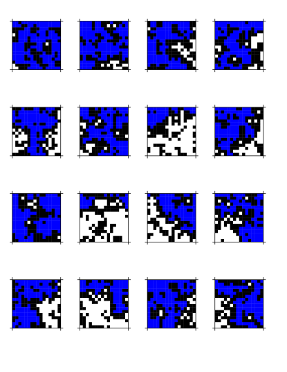
Figure 12: (Color online) Examples of the percolation pattern of local density for 32 different realizations with disorder strength $\Delta=25t$. 19 of the clusters are percolated. Clusters of size $L=16$, density $\rho=1.1$, and interaction $U=80t$.

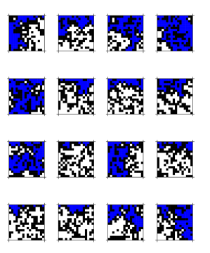
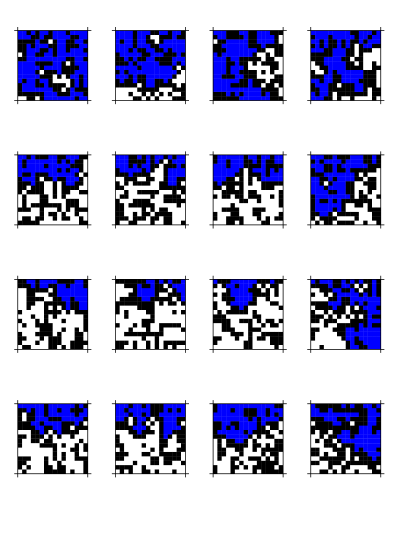
Figure 13: (Color online) Examples of the percolation pattern of local density for 32 different realizations with disorder strength $\Delta=30t$. 10 of the clusters are percolated. Clusters of size $L=16$, density $\rho=1.1$, and interaction $U=80t$.

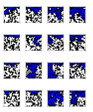
Figure 14: (Color online) Examples of the percolation pattern of local density for 32 different realizations with disorder strength $\Delta=35t$. 6 of the clusters are percolated. Clusters of size $L=16$, density $\rho=1.1$, and interaction $U=80t$.

References

- (1) H. A. Gersch and G. C. Knollman, Phys. Rev. 129, 959 (1963).
- (2) T. Giamarchi and H. J. Schulz, Phys. Rev. B 37, 325 (1988).
- (3) M. P. A. Fisher, P. B. Weichman, G. Grinstein, and D. S. Fisher, Phys. Rev. B 40, 546 (1989).
- (4) J. K. Freericks and H. Monien, Europhys. Lett. 26, 545 (1994).
- (5) R. T. Scalettar, G. G. Batrouni, and G. T. Zimanyi, Phys. Rev. Lett. 66, 3144 (1991).
- (6) W. Krauth, N. Trivedi, and D. Ceperley, Phys. Rev. Lett. 67, 2307 (1991).
- (7) S. Zhang, N. Kawashima, J. Carlson, and J. E. Gubernatis, Phys. Rev. Lett. 74, 1500 (1995).
- (8) L. Amico and V. Penna, Phys. Rev. Lett. 80, 2189 (1998).
- (9) I. Carusotto and Y. Castin, New J. Phys. 5, 91 (2003).
- (10) A. Priyadarshee, S. Chandrasekharan, J.-W. Lee, and H. U. Baranger, Phys. Rev. Lett. 97, 115703 (2006).
- (11) P. Hitchcock and E. S. Sørensen, Phys. Rev. B 73, 174523 (2006).
- (12) G. G. Batrouni, H. R. Krishnamurthy, K. W. Mahmud, V. G. Rousseau, and R. T. Scalettar, Phys. Rev. A 78, 023627 (2008).
- (13) G. Semerjian, M. Tarzia, and F. Zamponi, Phys. Rev. B 80, 014524 (2009).
- (14) W.-J. Hu and N.-H. Tong, Phys. Rev. B 80, 245110 (2009).
- (15) P. Anders, E. Gull, L. Pollet, M. Troyer, and P. Werner, Phys. Rev. Lett. 105, 096402 (2010).
- (16) A. Rançon and N. Dupuis, Phys. Rev. B 83, 172501 (2011).
- (17) H. Yokoyama, T. Miyagawa, and M. Ogata, J. Phys. Soc. Jpn. 80, 084607 (2011).
- (18) J. Kisker and H. Rieger, Phys. Rev. B 55, R11981(R) (1997).
- (19) J. Kisker and H. Rieger, Physica A 246, 348 (1997).
- (20) K. Sheshadri, H. R. Krishnamurty, R. Pandit, and T. V. Ramakrishnan, Europhys. Lett. 22, 257 (1993).
- (21) K. Hettiarachchilage, V. G. Rousseau, K.-M. Tam, M. Jarrell, and J. Moreno, Phys. Rev. A 87, 051607(R) (2013).
- (22) J. F. Dawson, F. Cooper, C.-C. Chien, and B. Mihaila, Phys. Rev. A 88, 023607 (2013).
- (23) M. Lacki, B. Damski, and J. Zakrzewski, Sci. Rep. 6, 38340 (2016).
- (24) S. G. Söyler, M. Kiselev, N. V. Prokof’ev, and B. V. Svistunov, Phys. Rev. Lett. 107, 185301 (2011).
- (25) H. Meier and M. Wallin, Phys. Rev. Lett. 108, 055701 (2012).
- (26) R. V. Pai, J. M. Kurdestany, K. Sheshadri, and R. Pandit, Phys. Rev. B 85, 214524 (2012).
- (27) Z. Yao, K. P. C. da Costa, M. Kiselev, and N. Prokof’ev Phys. Rev. Lett. 112, 225301 (2014).
- (28) K. G. Singh and D. S. Rokhsar, Phys. Rev. B 46, 3002 (1992).
- (29) J. P. Álvarez Zún̈iga and N. Laflorencie, Phys. Rev. Lett. 111, 160403 (2013).
- (30) D. van Oosten, P. van der Straten, and H. T. C. Stoof, Phys. Rev. A 63, 053601 (2001).
- (31) B. Capogrosso-Sansone, N. V. Prokof’ev, and B. V. Svistunov, Phys. Rev. B 75, 134302 (2007).
- (32) S. J. Thomson and F. Krüger, Europhys. Lett. 108, 300002 (2014).
- (33) R. Ng and E. S. Sørensen, Phys. Rev. Lett. 114, 255701 (2015).
- (34) A. E. Niederle and H. Rieger, New J. Phys. 15, 075029(2013).
- (35) F. Lin, E. S. Sørensen, and D. M. Ceperley, Phys. Rev. B 84, 094507 (2011).
- (36) L. Pollet, N.V. Prokof’ev, B. V. Svistunov, and M. Troyer, Phys. Rev. Lett. 103, 140402 (2009).
- (37) V. Gurarie, L. Pollet, N. V. Prokof’ev, B. V. Svistunov, and M. Troyer, Phys. Rev. B 80, 214519 (2009).
- (38) D. S. Fisher and M. P. A. Fisher, Phys. Rev. Lett. 61, 1847 (1988).
- (39) D. Finotello, K. A. Gillis, A. Wong, and M. H. W. Chan, Phys. Rev. Lett. 61, 1954 (1988).
- (40) P. A. Crowell, F. W. Van Keuls, and J. D. Reppy, Phys. Rev. B 55, 12620 (1997).
- (41) G. A. Csáthy, J. D. Reppy, and M. H. W. Chan, Phys. Rev. Lett. 91, 235301 (2003).
- (42) G. Agnolet, D. F. McQueeney, and J. D. Reppy, Phys. Rev. B 39, 8934 (1989).
- (43) D. J. Bishop and J. D. Reppy, Phys. Rev. Lett. 40, 1727 (1978).
- (44) I. Bloch, J. Dalibard, and W. Zwerger, Rev. Mod. Phys. 80, 885 (2008).
- (45) M. Greiner, O. Mandel, T. Esslinger, T. W. Hänsch, and I. Bloch, Nature 415, 39 (2002).
- (46) D. Jaksch, C. Bruder, J.I. Cirac, C.W. Gardiner, and P. Zoller, Phys. Rev. Lett. 81, 3108 (1998).
- (47) R. B. Griffiths, Phys. Rev. Lett. 23, 17 (1969).
- (48) M. Pasienski, D. McKay, M. White, and B. DeMarco, Nat. Phys. 6, 677 (2011).
- (49) A. Hegg, F. Krüger, and P. W. Phillips, Phys. Rev. B 88, 134206 (2013).
- (50) J. P. Álvarez Zúñiga, D. J. Luitz, G. Lemarié, and N. Laflorencie, Phys. Rev. Lett. 114, 155301 (2015).
- (51) P. B. Weichman and R. Mukhopadhyay, Phys. Rev. B 77, 214516 (2008).
- (52) A. Rodriguez, L. J. Vasquez, K. Slevin, and R. A. Römer, Phys. Rev. Lett. 105, 046403 (2010).
- (53) J. Lindinger and A. Rodríguez Phys. Rev. B 96, 134202 (2017).
- (54) K. Yakubo and M. Ono, Phys. Rev. B 58, 9767 (1998).
- (55) L. Ujfalusi and I. Varga, Phys. Rev. B 91, 184206 (2015).
- (56) C. Castellani, C. Di Castro, and L. Peliti, J. Phys. A 19, L1099 (1986).
- (57) F. Wegner, Z. Phys. B 35, 207 (1979).
- (58) F. Wegner, Z. Phys. B 36, 209 (1980).
- (59) G. Schubert, J. Schleede, K. Byczuk, H. Fehske, and D. Vollhardt, Phys. Rev. B 81, 155106 (2010).
- (60) C. W. Moore, K.-M. Tam, Y. Zhang, and M. Jarrell, arxiv:1707.04597.
- (61) V. G. Rousseau, Phys. Rev. E 77, 056705 (2008).
- (62) V. G. Rousseau, Phys. Rev. E 78, 056707 (2008).
- (63) V. G. Rousseau and D. Galanakis, arXiv:1209.0946 (2012).
- (64) V. G. Rousseau, Phys. Rev. B 90, 134503 (2014).
- (65) E. L. Pollock and D. M. Ceperley, Phys. Rev. B 36, 8343 (1987).
- (66) L. Wang, K. S. D. Beach, and A. W. Sandvik, Phys. Rev. B 73, 014431 (2006).
- (67) P. W. Anderson, Phys. Rev. 109, 1492 (1958).
- (68) A. MacKinnon, Rep. Prog. Phys. 56, 1469 (1993).
- (69) V. Dobrosavljević, A. A. Pastor, and B. K. Nikolić, Europhys. Lett. 62, 76 (2003).
- (70) C. E. Ekuma, H. Terletska, K.-M. Tam, Z.-Y. Meng, J. Moreno, and M. Jarrell, Phys. Rev. B 89, 081107 (2014).
- (71) M. Janssen, Phys. Rep. 295, 1 (1998).
- (72) A. Altland and M. R. Zirnbauer, Phys. Rev. B 55, 1142 (1997).
- (73) F. Evers and A. D. Mirlin, Rev. Mod. Phys. 80, 1355 (2008).
- (74) T. Nakayama, K. Yakubo, Fractal Concepts in Condensed Matter Physics, Springer, New York (2003).
- (75) H. E. Stanley and P. Meakin, Nature. 335, 405 (1988).
- (76) H. Salat, R. Murcio, and E. Arcaute, Physica A 473, 467 (2017).
- (77) L. A. Saravia, F1000Research 3:14 (2014).
- (78) L. A. Saravia, A. Giorgi, and F. Momo, Oikos 121, 1810 (2012).
- (79) A. Chhabra and R. V. Jensen, Phys. Rev. Lett. 62, 1327 (1989).
- (80) T. C. Halsey, M. H. Jensen, L. P. Kadanoff, I. Procaccia, and B. I. Shraiman, Phys. Rev. A 33, 1141 (1986).
- (81) D. Stošić, T. Stošić, and H. E. Stanley, Physica A, 428, 13 (2005).
- (82) L. Zhao, W. Li , C. Yang, J. Han, Z. Su, and Y. Zhou, PLOS ONE 12(1): e0170467 (2017).
- (83) P. Buonsante, F. Massel, V. Penna, and A. Vezzani, Phys. Rev. A 79, 013623 (2009).
- (84) L. Dell’Anna and M. Fabrizio, J. Stat. Mech. 11, P08004 (2011).
- (85) K. Sheshadri, H. R. Krishnamurthy, R. Pandit, and T. V. Ramakrishnan, Phys. Rev. Lett. 75, 4075 (1995).
- (86) A. Barman, S. Dutta, A. Khan, and S. Basu, Eur. Phys. J. B, 86, 308 (2013).
- (87) J.-M. Gao, R.-A. Tang, and J.-K. Xue, Europhys. Lett. 117, 60007 (2017).
- (88) S. Kirkpatrick, Rev. Mod. Phys. 45, 574 (1973).
- (89) V. K. S. Shante and S. Kirkpatrick, Adv. Phys. 20, 325 (1971).
- (90) Y. Wang, W. Guo, and A. W. Sandvik, Phys. Rev. Lett. 114, 105303 (2015).