A worldwide model for boundaries of urban settlements

Abstract

The shape of urban settlements plays a fundamental role in their sustainable planning. Properly defining the boundaries of cities is challenging and remains an open problem in the Science of Cities. Here, we propose a worldwide model to define urban settlements beyond their administrative boundaries through a bottom-up approach that takes into account geographical biases intrinsically associated with most societies around the world, and reflected in their different regional growing dynamics. The generality of the model allows to study the scaling laws of cities at all geographical levels: countries, continents, and the entire world. Our definition of cities is robust and holds to one of the most famous results in Social Sciences: Zipf’s law. According to our results, the largest cities in the world are not in line with what was recently reported by the United Nations. For example, we find that the largest city in the world is an agglomeration of several small settlements close to each other, connecting three large settlements: Alexandria, Cairo, and Luxor. Our definition of cities opens the doors to the study of the economy of cities in a systematic way independently of arbitrary definitions that employ administrative boundaries.

I Introduction

What are cities? In The Death and Life of the Great American Cities, Jacobs argues that human relations can be seen as a proxy for places within cities jacobs1961 . A modern view of cities establishes that they can be defined by the interactions among several types of networks batty2013 ; west2017 , from infrastructure networks to social networks. In recent years, an increasing number of studies have been proposed to define cities through consistent mathematical models makse1995 ; makse1998 ; rozenfeld2008 ; rozenfeld2011 ; rybski2013 ; murcio2013 ; hernando2014 ; frasco2014 ; arcaute2014 ; masucci2015 ; arcaute2016 ; fluschnik2016 and to investigate urban indicators at inter- and intra-city scales, in order to shed some light on problems faced by decision makers bettencourt2007 ; arbesman2009 ; bettencourt2010a ; bettencourt2010b ; gomez-lievano2012 ; gallos2012a ; bettencourt2013 ; fragkias2013 ; oliveira2014 ; melo2014 ; louf2014 ; alves2015 ; li2015 ; hanley2016 ; caminha2017 ; operti2017 . Despite the efforts of such studies, to properly defining the boundaries of urban settlements remains an open problem in the Science of Cities. A minimum criterion of acceptability for any model of cities seems to be the one that retrieves a conspicuous scaling law found for United States (US), United Kingdom (UK), and other countries, known as Zipf’s law rozenfeld2008 ; rozenfeld2011 ; gabaix1999a ; gabaix1999b ; ioannides2003 ; cordoba2008 ; giesen2010 ; giesen2011 ; jiang2011 ; giesen2012 ; ioannides2013 ; duraton2014 ; watanabe2015 .

In 1949, Zipf zipf1949 observed that the frequency of words used in the English language obeys a natural and robust power law behavior, i.e. a few words are used many times, while many words are used just a few times. Zipf’s law can be represented generically by the following relation between the size $S$ of objects from a given set and its rank $R$:

$$R\propto S^{-\zeta},$$ (1)

where $\zeta=1$ is Zipf’s exponent. The size of objects is, in the original context, the frequency of used words. On the other hand, if such objects are cities, then the sizes stand for the population of each city, taking into account Zipf’s law and reflecting the fact that there are more small towns than metropolises in the world. We emphasize that it is not straightforward that the Zipf’s law, despite its robustness, should hold independently of the city definition, since other scaling relations are not, such as the allometric exponents for CO₂ emissions and light pollution oliveira2014 ; operti2017 . Many other man-made and natural phenomena also exhibit the same persistent result, e.g. earthquakes and incomes sornette1996 ; okuyama1999 .

Here, we propose a worldwide model to define urban settlements beyond their usual administrative boundaries through a bottom-up approach that takes into account cultural, political, and geographical biases naturally embedded in the population distribution of continental areas. After all, it is not surprising that two regions, e.g. one in western Europe and another one in eastern Asia, spatially contiguous in population or in commuting level have different cultural, political or geographical characteristics. Thus, it is also not surprising that such issues yield different stages of the same mechanics of growth. The main goal of our model is to be successful in defining cities even in large regions. Our conjecture is straightforward: there are hierarchical mechanisms, similar to those present in previous studies of cities in the UK arcaute2016 and brain networks gallos2012b , behind the growth and innovation of urban settlements. These mechanisms are ruled by a combination of general measures, such as the population and the area of each city, and intrinsic factors which are specific to each region, e.g. topographical heterogeneity, political and economic issues, and cultural customs and traditions. In other words, if political turmoil or economic recession plagues a metropolis for a long time, all of its satellites are affected too, i.e. the entire region ruled by the metropolis will be negatively impacted.

II The models

II.1 City Clustering Algorithm (CCA)

In 2008, Rozenfeld et al. rozenfeld2008 proposed a model to define cities beyond their usual administrative boundaries using a notion of spatial continuity of urban settlements, called the City Clustering Algorithm (CCA) rozenfeld2008 ; rozenfeld2011 ; rybski2013 ; oliveira2014 ; frasco2014 ; fluschnik2016 ; caminha2017 ; operti2017 . The CCA is defined for discrete or continuous landscapes rozenfeld2011 by two parameters: a population density threshold $D^{*}$ and a distance threshold $\ell$. These parameters describe the populated areas and the commuting distance between areas, respectively. Here, we adopt the following strategy to improve the discrete CCA performance: (i) Supposing a regular rectangular lattice $L_{x}\times L_{y}$ of sites where the population density of the $k$-th site is $D_{k}$, we perform an initial agglomeration by $D^{*}$ to identify all clusters. If $D_{k}>D^{*}$, then the $k$-th site is populated and we aggregate it with its populated nearest neighbors. Otherwise, the $k$-th site is unpopulated. (ii) For each populated cluster, we define its shell sites, i.e. sites in the interface between populated and unpopulated areas. (iii) Lastly, we perform a final agglomeration by $\ell$, taking into account only the shell sites. If $d_{ij}<\ell$, where $d_{ij}$ is the distance between the $i$-th and $j$-th shell sites, and if they belong to different clusters, then the $i$-th and $j$-th sites belong to the same CCA cluster, even with spatial discontinuity. Otherwise, they indeed belong to different CCA clusters. This simple strategy improves the algorithm’s computational performance because the number of shell sites is proportional to $L$, where $L=L_{x}\approx L_{y}$ is a linear measure of the lattice.

II.2 City Local Clustering Algorithm (CLCA)

We propose a worldwide model based on the CCA, called the City Local Clustering Algorithm (CLCA), not only to define cities beyond their usual administrative boundaries, but also to take into account the intrinsic cultural, political and geographical biases associated with most societies and reflected in their particular growing dynamics. The traditional CCA, with fixed $\ell$ and $D^{*}$, when applied to a large population density map, can introduce biases defining a lot of clusters in some regions, while in others just a few. We present the CLCA with the aim of defining cities even in large regions in order to overcome such CCA weakness. Hence, it is possible that other models, such as the models based on street networks proposed by Masucci et al. masucci2015 and Arcaute et al. arcaute2016 , carry the same CCA burden and that local adaptations are necessary for their applications into large regions.

The main idea of ​​our model is to analyze the change of the CCA clusters through the variation of $D^{*}$ under the perspective of different regions. First, we define a regular rectangular lattice $L_{x}\times L_{y}$ of sites, where the population density of the $k$-th site is $D_{k}$. We sort all the sites in a list according to the population density, in descending order. Therefore, the site with the greatest population density is the first entry in this list, which we call the first reference site. The reference site can be considered as the current core of the analyzed region. Second, we apply the CCA to the lattice, keeping a fixed value of $\ell$, for a range of $D^{*}$ decreasing from a maximum value $D^{(max)}$ to a minimum value $D^{(min)}$ with a decrement $\delta$. During the decreasing of $D^{*}$, clusters are formed and they spread out to all regions of the lattice. Eventually, the cluster that contains the reference site (from now on the reference cluster), together with one or more of the other clusters, will merge from $D^{(i)}$ to $D^{(i+1)}$, where $D^{(i+1)}=D^{(i)}-\delta$. In order to accept or deny the merging of these clusters, we introduce three conditions:

1. If the area $A_{r}(D^{(i)})$ of the reference cluster $r$, i.e. the cluster that contains the $r$-th reference site at $D^{(i)}$, obeys

   $$A_{r}(D^{(i)})<A^{*},$$ (2)

   then the reference cluster $r$ always merges with other clusters, because it is still considered very small. In this context, the area $A^{*}$ can be understood as the minimal area of a metropolis.

2. If the difference between the areas of the reference cluster $r$ at $D^{(i+1)}$ and $D^{(i)}$ obeys

   $$A_{r}(D^{(i+1)})-A_{r}(D^{(i)})>H^{*}A_{r}(D^{(i)}),$$ (3)

   then the reference cluster $r$ has grown without merging (Fig.1a) or there is a merging of at least two large clusters (Fig.1b). In the last case, we emphasize that if there are more than two clusters involved in the merging process, the reference cluster $r$ may not be one of the largest. As the first case is not desirable, we can avoid it by reducing the value of $\delta$ and keeping the value of $H^{*}$ relatively high. The parameter $H^{*}$ can be understood as the percentage of the area of the reference cluster $r$ at $D^{(i)}$. If the second case happens, we consider the entire region inside of the reference cluster $r$ at $D^{(i+1)}$, but the clusters of this region (which we call the usual clusters) are defined by those at $D^{(i)}$. The usual clusters are the CCA clusters at the imminence of the merging process between $D^{(i)}$ and $D^{(i+1)}$. This includes the reference cluster $r$ itself and one or more of the other clusters before the merging (Fig.1b). Furthermore, all of the sites of the reference cluster $r$ at $D^{(i+1)}$ are removed from the initial list of reference sites. This condition is necessary because we should not merge two large metropolises.

3. In condition (ii), when a reference cluster $r$ is merging with another cluster that covers one or more regions already defined by previous reference clusters at different values of $D^{*}$, there is a strong likelihood of the emergence of a forbidden region within that cluster. In this case, we force the region already defined by the largest value of $D^{*}$ to grow to the limits of the forbidden region (Fig.1c). The forbidden regions are the complementary areas of the reference clusters already defined within the usual clusters. As a consequence of this procedure, some CCA clusters that were hidden after the analysis of the previous reference cluster arise in this forbidden region. We justify this condition by the idea that a metropolis rules the growth of its satellites, since it plays a fundamental role in their socioeconomic relations.

We apply the same procedure to the second reference cluster, to the third reference cluster, and so on. Finally, we also define the isolated clusters with the minimum value of $D^{*}$ for all the cases accepted in condition (ii). In order to make our model clearer, we chose the descending order to sort the population density for one reason: To favor the merging process of the high density clusters that rose from the decreasing of the $D^{*}$. In practice, we run our revised discrete CCA just once for the entire range of input parameters and store all of the outputs in order to improve the performance of the model. The apparent simplicity of this task hides a RAM memory management problem of storing all of the outputs in a medium-performance computer. We overcome such a barrier through the zram module zram2017 , available in the newest linux kernels. The zram module creates blocks which compress and store information dynamically in the RAM memory itself, at the cost of processing time.

III The dataset

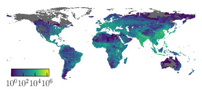
Figure 2: (Color online) The Global Rural-Urban Mapping Project (GRUMPv1) dataset. The population map of the entire world from the GRUMPv1 dataset in logarithmic scale.

We use the Global Rural-Urban Mapping Project (GRUMPv1) grump2011 , available from the Socioeconomic Data and Applications Center (SEDAC) at Columbia University, to apply the CLCA to a single global dataset. The GRUMPv1 dataset is composed of georeferenced rectangular population grids for 232 countries around the world in the year 2000 (Fig. 2). Such a dataset is a compilation of gridded census and satellite data for the populations of urban and rural areas. These data are provided at a high resolution of $30\;\text{arc-seconds}$, equivalent to $30/3600\;\text{degrees}$ or a grid of $0.926\;km\times 0.926\;km$ at the Equator. We note that despite of the heterogeneous population distributions that built the GRUMPv1, its overall resolution is tolerable to the CLCA, since we can identify well-defined clusters around all continents in the raw data.

We calculate the area of ​​each site by the composition of two spherical triangles snyder1987 . The area of a spherical triangle with edges $a$, $b$ and $c$ is given by

$$A=4R_{e}^{2}\tan^{-1}\left[\tan\left(\frac{s}{2}\right)\tan\left(\frac{s_{a}}{2}\right)\tan\left(\frac{s_{b}}{2}\right)\tan\left(\frac{s_{c}}{2}\right)\right]^{1/2},$$ (4)

where $s=(a/R_{e}+b/R_{e}+c/R_{e})/2$, $s_{a}=s-a/R_{e}$, $s_{b}=s-b/R_{e}$, and $s_{c}=s-c/R_{e}$. In this formalism, $R_{e}=6,378.137\;km$ is the Earth’s radius and the edge lengths are calculated by the great circle (geodesic) distance between two points $i$ and $j$ on the Earth’s surface:

$$d_{ij}=R_{e}\cos^{-1}[\sin(\phi_{i})\sin(\phi_{j})+\cos(\phi_{i})\cos(\phi_{j})\cos(\lambda_{j}-\lambda_{i})].$$ (5)

The values of $\lambda_{i}$ ($\lambda_{j}$) and $\phi_{i}$ ($\phi_{j})$, measured in radians, are the longitude and latitude, respectively, of the point $i$ ($j$). Thus, we are able to define the population density for each site of the lattice, since its population and area are known.

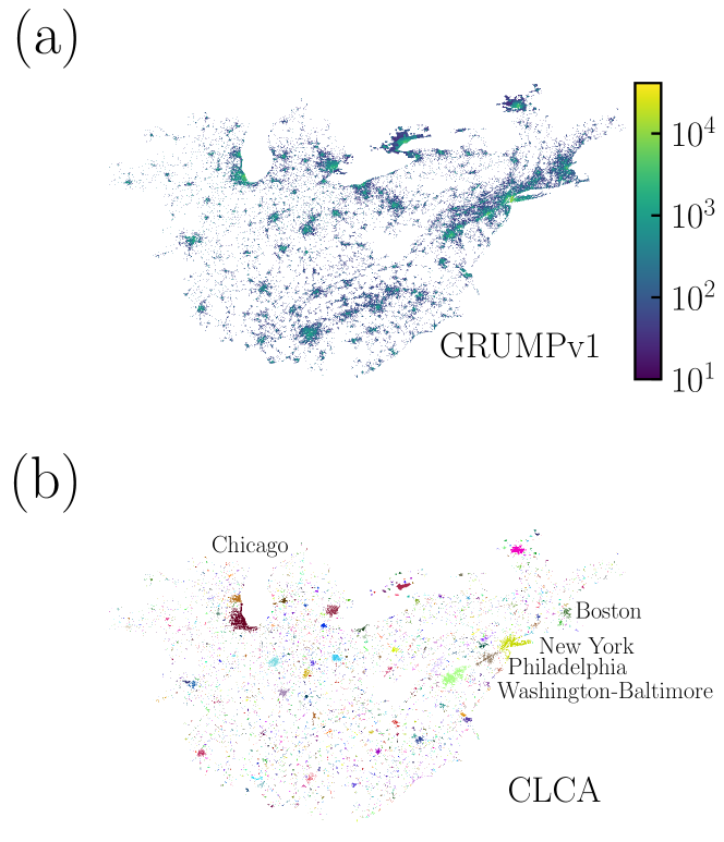
Figure 3: (Color online) The largest cluster of regions for the United States (US). (a) The single population density cluster from the Eastern US is defined by the City Clustering Algorithm (CCA) with lower and upper bound parameters $D^{*}=50\;\text{people}/km^{2}$ and $\ell=10\;km$, respectively. The population, provided by the Global Rural-Urban Mapping Project (GRUMPv1) dataset, is shown in logarithmic scale within each populated area. (b) Application of the City Local Clustering Algorithm (CLCA) for the cluster of regions of the Eastern US. The CLCA cities are represented in several colors, e.g. New York in mustard, Philadelphia in light brown, Washington-Baltimore in light green, Boston in green and Chicago in red. The CLCA parameters used were $D^{(min)}=100\;\text{people}/km^{2}$, $D^{(max)}=1000\;\text{people}/km^{2}$, $\delta=10\;\text{people}/km^{2}$, $\ell=3\;km$, $A^{*}=50\;km^{2}$, and $H^{*}=0.05$.

We also pre-process the GRUMPv1 dataset, dividing all countries and continents — and even the entire world — into large regions which we call clusters of regions, to apply our model in a feasible computational time using medium-performance computers. These regions are defined by the CCA with lower and upper bound parameters $D^{*}=50\;\text{people}/km^{2}$ and $\ell=10\;km$, respectively. We believe that such large clusters can hold the socioeconomic and cultural relations among different urban settlements of a territory. Fig. 3a shows the largest clusters of regions in the US; as we can see, all of the Eastern US is considered a single cluster.

IV Results

To show the relevance of our model, we apply the CLCA to the GRUMPv1 dataset at three different geographic levels: countries, continents and the entire world. For each case, we consider only a single set of CLCA parameters. We justify our choices with the following assumptions: (i) $D^{(min)}=100\;\text{people}/km^{2}$, a value slightly greater than the lower bound CCA parameter ($D^{*}=50\;\text{people}/km^{2}$) used to define the regions of clusters; (ii) $D^{(max)}=1000\;\text{people}/km^{2}$, a loosened value of $D^{(max)}=\infty$; (iii) $\delta=10\;\text{people}/km^{2}$, a small enough value to avoid the reference clusters growing without merging; (iv) $\ell=3\;km$, the critical distance threshold, already extensively analyzed by previous CCA studies rozenfeld2008 ; rozenfeld2011 ; oliveira2014 ; (v) $A^{*}=50\;km^{2}$, the minimum area of a metropolis, as it is required that $A^{*}$ be reasonably greater than the minimum unit of area from the dataset and smaller than a metropolis’ area; and (vi) $H^{*}=0.05$, a large enough value to favor the merging of clusters which are similar in size. The Fig. 3b shows the CLCA cities defined by the single set of CLCA parameters. For other regions, see the Supplementary Information (SI).

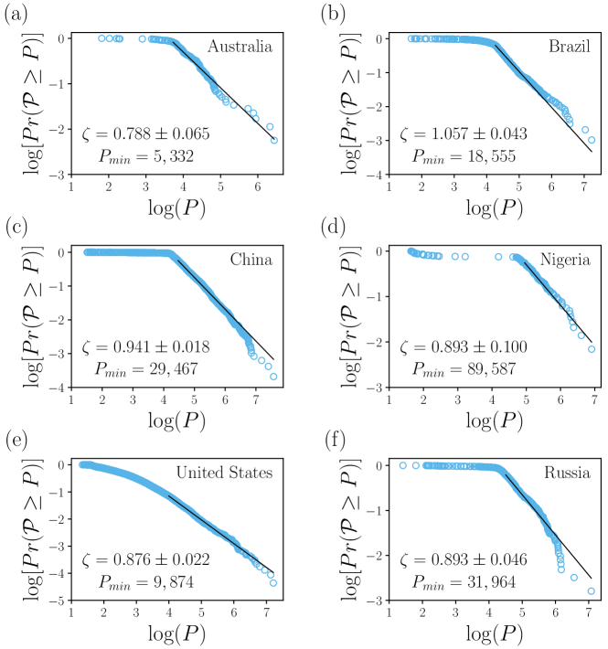
Figure 4: (Color online) Cumulative Distribution Function (CDF) $Pr(\mathcal{P}\geq P)$ versus population $P$, in log-log scale, for the countries with the highest number of cities in each continent (for other countries, see the SI). (a)-(f) Cities proposed by the City Local Clustering Algorithm (CLCA) are represented by light blue circles. The solid black line is the maximum likelihood power-law fit defined by the Maximum Likelihood Estimator (MLE) clauset2009 . The value of the lower bound $P_{min}$ and the exponent $\zeta$ are also shown. The CLCA parameters used were $D^{(min)}=100\;\text{people}/km^{2}$, $D^{(max)}=1000\;\text{people}/km^{2}$, $\delta=10\;\text{people}/km^{2}$, $\ell=3\;km$, $A^{*}=50\;km^{2}$ and $H^{*}=0.05$.

We study the population distribution using the Maximum Likelihood Estimator (MLE) proposed by Clauset et al. clauset2009 . Their approach combines maximum-likelihood fitting methods with goodness-of-fit tests based on Kolmogorov-Smirnov (KS) statistic. The Fig. 4 shows the log-log behavior of the Cumulative Distribution Function (CDF) for the population of the CLCA cities, considering only the countries with the highest number of CLCA cities for each continent (for other countries, see the SI). The $Pr(\mathcal{P}\geq P)$ represents the probability that a random population $\mathcal{P}$ takes on a value greater or equal to the population $P$. In all CDF plots, we also show the maximum likelihood power-law fit, as well as, the value of the exponent $\zeta=\alpha-1$, where $\alpha$ is the MLE exponent, and the value of $P_{min}$, the lower bound of the MLE.

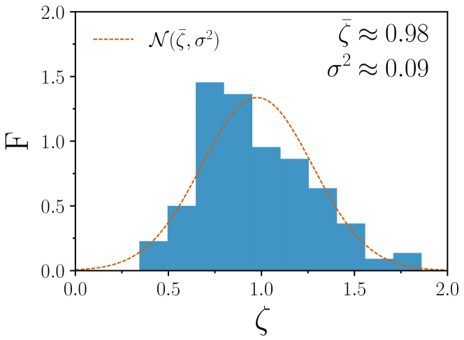
Figure 5: (Color online) Normalized histogram, with frequency $F$, of the $\zeta$ exponent at the country level. The plot shows those countries (145 out of 232) with at least 10 cities defined by the City Local Clustering Algorithm (CLCA) in the region covered by the maximum likelihood power-law fit. We find the mean value of the Zipf’s exponents $\bar{\zeta}=0.98$ and its variance $\sigma^{2}=0.09$. The dashed red line stands for the normal distribution $\mathcal{N}(\bar{\zeta},\sigma^{2})$. Therefore, Zipf’s law holds for the most countries.

In Fig. 5, we show a normalized histogram, with frequency $F$, of the $\zeta$ exponents for all countries ( 145 out of 232) with at least 10 CLCA cities in the region covered by the maximum likelihood power-law fit. The mean value of the $\zeta$ exponents is $\bar{\zeta}=0.98$, with variance $\sigma^{2}=0.09$. The dashed red line stands for the normal distribution $\mathcal{N}(\bar{\zeta},\sigma^{2})$. In spite of the $\zeta$ exponent heterogeneity illustrated by Fig. 5, Zipf’s law holds for most countries around the globe. We emphasize that such results corroborate with previous studies performed for one country or a small number of countries rozenfeld2008 ; rozenfeld2011 ; gabaix1999a ; gabaix1999b ; ioannides2003 ; cordoba2008 ; giesen2010 ; giesen2011 ; jiang2011 ; giesen2012 ; ioannides2013 ; duraton2014 ; watanabe2015 . In special, the Fig. 5 also endorses an astute meta-analysis performed by Cottineau cottineau2017 . Cottineau provided a comparison among the Zipf’s law exponents found in 86 studies. Our results strongly corroborate those presented in such study, except that our exponents are ranged between 0 and 2.

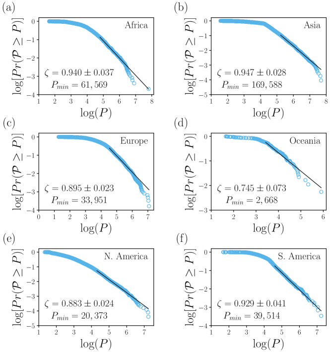
Figure 6: (Color online) Cumulative Distribution Function (CDF) $Pr(\mathcal{P}\geq P)$ versus population $P$, in log-log scale, for the continents. (a)-(f) Cities proposed by the City Local Clustering Algorithm (CLCA) are represented by light blue circles. The solid black line is the maximum likelihood power-law fit defined by the Maximum Likelihood Estimator (MLE) clauset2009 . The value of the lower bound $P_{min}$ and the exponent $\zeta$ are also shown. The CLCA parameters used were $D^{(min)}=100\;\text{people}/km^{2}$, $D^{(max)}=1000\;\text{people}/km^{2}$, $\delta=10\;\text{people}/km^{2}$, $\ell=3\;km$, $A^{*}=50\;km^{2}$ and $H^{*}=0.05$.

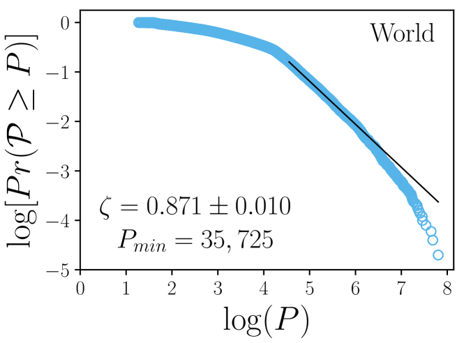
Figure 7: (Color online) Cumulative Distribution Function (CDF) $Pr(\mathcal{P}\geq P)$ versus population $P$, in log-log scale, for the entire world. (a)-(f) Cities proposed by the City Local Clustering Algorithm (CLCA) are represented by light blue circles. The solid black line is the maximum likelihood power-law fit defined by the Maximum Likelihood Estimator (MLE) clauset2009 . The value of the lower bound $P_{min}$ and the exponent $\zeta$ are also shown. The CLCA parameters used were $D^{(min)}=100\;\text{people}/km^{2}$, $D^{(max)}=1000\;\text{people}/km^{2}$, $\delta=10\;\text{people}/km^{2}$, $\ell=3\;km$, $A^{*}=50\;km^{2}$ and $H^{*}=0.05$.

Furthermore, we challenge the robustness of our model at higher geographic levels: continents and the entire world. We performed the same analyses and find that our results persist on both scales, i.e. the CLCA cities follows Zipf’s law for continents and the entire world, as illustrated in Figs. 6 and 7.

We summarize our results in a set of 7 tables: Tables LABEL:t_countries_af, LABEL:t_countries_as, LABEL:t_countries_eu, LABEL:t_countries_na , LABEL:t_countries_oc, and LABEL:t_countries_sa, for countries from Africa; Asia; Europe; North America; Oceania; and South America, respectively. Table LABEL:t_continents_world contains similar information for all continents and the entire world. In all cases, we show the name of the considered region (country, continent or globe), the ISO 3166-1 alpha-3 code associated (only for countries), the number of cities obtained by the CLCA and those covered by the MLE, the lower bound $P_{min}$, and the Zipf’s exponent $\zeta$.

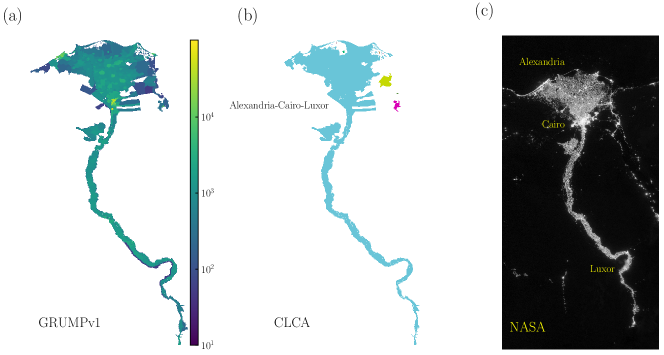
Figure 8: (Color online) Northeastern region of Egypt. (a) The cluster of regions defined by the pre-processing of the GRUMPv1 dataset for the Northeastern region of Egypt. (b) The largest city defined by the City Local Clustering Algorithm (CLCA) in the entire world is formed by several cities, including Alexandria, Cairo, and Luxor. (c) Night-time lights of the Northeast of Egypt provided by National Aeronautics and Space Administration (NASA). The CLCA cities found exhibit a remarkable similarity with the lights across the Nile.

It is remarkable that the top CLCA city, with a population of 63,585,039 people, is composed of three large urban settlements (Alexandria, Cairo, and Luxor) connected by several small ones. Figs. 8a, 8b, and 8c show the largest cluster of regions in Egypt for the GRUMPv1 dataset; CLCA cities; and night-time lights from the National Aeronautics and Space Administration (NASA) nasa2016 , respectively. We believe the main reason for this finding has been present in the Northeast of Africa since before the beginning of ancient civilization — namely, the Nile river. Actually, it is well known that almost the entire Egypt population lives in a strip along the Nile river, in the Nile delta, and in the Suez canal on 4% of the total country area ($~{}10^{6}\;km^{2}$), where there are arable lands to produce food gehad2003 . The river and delta regions are composed by some large cities and a lot of small villages, making them extremely dense. Therefore, our results raise the hypothesis that the cities and villages across the Nile can be seen as a kind of “megacity”, despite spatially non-contiguous, due to the socioeconomic relation, reflected on the high commuting levels, among close subregions.

The Table LABEL:t_world shows the top 25 CLCA cities in the entire world by population, and their associated areas. After the top CLCA city, Alexandria-Cairo-Luxor, we emphasize that the 13 next-largest CLCA cities are in Asia. Indeed, we can see that the shape of the tail end of the entire world population distribution (in Fig. 7) is roughly ruled by the greater CLCA city in Africa and several CLCA cities in Asia.

These facts are not in line with what was recently reported by the United Nations (UN) un2016 , e.g. the largest CLCA city, Alexandria-Cairo-Luxor, is just the 9th largest city according to the UN, and the largest UN city, Tokyo, is just the 4th largest according to our analyses.

V Conclusions

We propose a model to define urban settlements through a bottom-up approach beyond their usual administrative boundaries, and moreover to account for the intrinsic cultural, political, and geographical biases associated with most societies and reflected in their particular growing dynamics. We claim that such a property qualifies our model to be applied worldwide, without any regional restrictions. We also propose an alternative strategy to improve the computational performance of the discrete CCA. We emphasize that the CCA can still be used to define cities; however, it depends upon a different tuning of its parameters for each large region without direct socioeconomic and political relations. Furthermore, we show that the definition of cities proposed by our approach is robust and holds to one of the most famous results in Social Science, Zipf’s law, not only for previously studied countries, e.g. the US, the UK, or China, but for all countries (145 from 232 provided by GRUMPv1) around the world. We also find that Zipf’s law emerges at different geographic levels, such as continents and the entire world. Another highlight of our study is the fact that our model is applied upon one single dataset to define all cities. Furthermore, we find that the most populated cities are not the major players in the global economy (such as New York City, London, or Tokyo). The largest CLCA city, with a population of 63,585,039 people, is an agglomeration of several small cities close to each other which connects three large cities: Alexandria, Cairo, and Luxor. Finally, after the top CLCA city of Alexandria-Cairo-Luxor, we find that the next-largest 13 CLCA cities are in Asia. These facts are not in full agreement with a recent UN report un2016 . According to our results, the largest CLCA city, Alexandria-Cairo-Luxor, is just the 9th largest city according to the UN, while the largest UN city, Tokyo, is just the 4th largest according to our analyses.

VI Data Accessibility

The dataset supporting this article are available at http://sedac.ciesin.columbia.edu/data/collection/grump-v1. More specifically, the reader can click on “Data sets” and, after that, on “Population Count Grid, v1 (1990,1995,2000)”. We also provide the codes for the proposed model that are available at https://doi.org/10.5061/dryad.968nq8n.

VII Competing Interests

We have no competing interests.

VIII Author’s Contributions

EAO performed the data analysis, the algorithm of the proposed model, and the statistical analysis. He also participated in the design of the study and drafted the manuscript. VF carried out the funding acquisition and helped draft the manuscript. JSA participated in the design of the study, carried out the funding acquisition, and helped draft the manuscript. HAM conceived, designed, and coordinated the research, as well as, carried out the funding acquisition and helped draft the manuscript. All authors approved the manuscript.

IX Acknowledgements

We thank the Global Rural-Urban Mapping Project (GRUMPv1) team for the dataset provided. Furthermore, we would like to thank X. Gabaix for helpful comments and discussions.

X Funding

We gratefully acknowledge funding by CNPq, CAPES, FUNCAP, NSF, and ARL Cooperative Agreement Number W911NF-09-2-0053 (the ARL Network Science CTA).

Figure 1: (Color online) City Local Clustering Algorithm (CLCA): Representation of the conditions (ii) and (iii). (a) The growth of the reference cluster without the merging process. (b) The rising of the usual clusters. The usual clusters are the CCA clusters at the imminence of the merging process between $D^{(i)}$ and $D^{(i+1)}$. (c) For $t$-th, $s$-th, and $r$-th reference clusters ($t$-th is prior to $s$-th which is prior to $r$-th), the merging processes are performed as described in (b), even though there are clusters already defined close to and within the current analysed region in the second and third case, respectively. In the latter, there is the emergence of a forbidden region. The forbidden regions are the complementary areas of the reference clusters already defined within the usual clusters. In order to define the clusters inside those areas, we force the region defined by the largest value of $D^{*}$ to grow to the limits of the forbidden region. Here, we suppose that $D^{(j)}>D^{(k)}$. The filled dots stand for the reference sites.

Table 1: African countries. We show the name, the ISO 3166-1 alpha-3 code, the number of cities obtained by the City Local Clustering Algorithm (CLCA) and the number of those covered by the maximum likelihood power-law fit defined by the Maximum Likelihood Estimator (MLE) clauset2009 (represented by $\dagger$), the lower bound $P_{min}$, and the Zipf’s exponent $\zeta$.

Country	ISO	CLCA cities	CLCA cities†	$P_{min}$	$\zeta$
Angola	AGO	20	16	43,937	0.780 $\pm$ 0.195
Benin	BEN	40	30	12,607	0.780 $\pm$ 0.142
Burkina Faso	BFA	139	78	12,314	1.256 $\pm$ 0.142
Botswana	BWA	79	58	1,674	0.785 $\pm$ 0.103
Central African Republic	CAF	37	11	14,868	1.230 $\pm$ 0.371
Ivory Coast	CIV	83	47	18,400	0.962 $\pm$ 0.140
Cameroon	CMR	143	93	7,478	0.711 $\pm$ 0.074
Democratic Republic of the Congo	COD	191	47	25,996	0.764 $\pm$ 0.111
Congo	COG	21	18	17,673	1.050 $\pm$ 0.248
Comoros	COM	16	15	4,167	0.922 $\pm$ 0.238
Cape Verde	CPV	16	11	5,205	1.083 $\pm$ 0.327
Algeria	DZA	273	112	24,192	0.910 $\pm$ 0.086
Egypt	EGY	19	12	11,967	0.511 $\pm$ 0.147
Eritrea	ERI	27	12	6,559	0.730 $\pm$ 0.211
Ethiopia	ETH	244	147	6,638	0.688 $\pm$ 0.057
Gabon	GAB	33	27	3,108	0.844 $\pm$ 0.162
Ghana	GHA	95	25	54,662	1.145 $\pm$ 0.229
Guinea	GIN	34	13	40,118	1.234 $\pm$ 0.342
Gambia	GMB	35	33	1,186	0.610 $\pm$ 0.106
Guinea-Bissau	GNB	26	14	9,148	1.139 $\pm$ 0.305
Kenya	KEN	179	20	72,756	1.383 $\pm$ 0.309
Liberia	LBR	42	19	6,468	0.604 $\pm$ 0.139
Libyan Arab Jamahiriya	LBY	30	18	40,273	1.180 $\pm$ 0.278
Lesotho	LSO	14	11	1,999	0.651 $\pm$ 0.196
Morocco (includes Western Sahara)	MAR	58	50	26,325	0.763 $\pm$ 0.108
Madagascar	MDG	138	74	14,867	1.340 $\pm$ 0.156
Mali	MLI	152	146	4,463	1.161 $\pm$ 0.096
Mozambique	MOZ	127	14	128,214	1.861 $\pm$ 0.497
Malawi	MWI	179	72	4,194	0.779 $\pm$ 0.092
Namibia	NAM	31	17	12,467	1.637 $\pm$ 0.397
Niger	NER	58	36	10,717	0.753 $\pm$ 0.126
Nigeria	NGA	144	80	89,587	0.893 $\pm$ 0.100
Sudan	SDN	77	56	39,764	1.031 $\pm$ 0.138
Senegal	SEN	42	34	13,475	0.798 $\pm$ 0.137
Sierra Leone	SLE	62	52	1,899	0.612 $\pm$ 0.085
Chad	TCD	75	14	19,574	1.086 $\pm$ 0.290
Togo	TGO	54	11	82,964	1.667 $\pm$ 0.503
Tunisia	TUN	46	36	16,130	1.014 $\pm$ 0.169
United Republic of Tanzania	TZA	114	33	73,621	0.936 $\pm$ 0.163
Uganda	UGA	155	33	30,587	1.386 $\pm$ 0.241
South Africa	ZAF	1,915	97	53,320	1.270 $\pm$ 0.129
Zambia	ZMB	55	34	7,118	0.666 $\pm$ 0.114
Zimbabwe	ZWE	28	24	13,411	0.746 $\pm$ 0.152

Table 2: Asian countries. We show the name, the ISO 3166-1 alpha-3 code, the number of cities obtained by the City Local Clustering Algorithm (CLCA) and the number of those covered by the maximum likelihood power-law fit defined by the Maximum Likelihood Estimator (MLE) clauset2009 (represented by $\dagger$), the lower bound $P_{min}$, and the Zipf’s exponent $\zeta$.

Country	ISO	CLCA cities	CLCA cities†	$P_{min}$	$\zeta$
Afghanistan	AFG	95	38	29,242	0.809 $\pm$ 0.131
Armenia	ARM	41	19	17,088	1.256 $\pm$ 0.288
Azerbaijan	AZE	34	21	17,169	0.776 $\pm$ 0.169
Bangladesh	BGD	103	58	26,586	0.581 $\pm$ 0.076
Bhutan	BTN	19	15	893	0.469 $\pm$ 0.121
China	CHN	4,782	2,706	29,467	0.941 $\pm$ 0.018
Cyprus	CYP	17	15	626	0.486 $\pm$ 0.126
Georgia	GEO	52	38	6,526	0.765 $\pm$ 0.124
Indonesia	IDN	2,416	542	12,876	0.894 $\pm$ 0.038
India	IND	1,040	299	94,976	0.786 $\pm$ 0.045
Iran	IRN	169	56	100,763	1.194 $\pm$ 0.160
Israel	ISR	24	20	877	0.448 $\pm$ 0.100
Jordan	JOR	13	11	15,253	0.803 $\pm$ 0.242
Japan	JPN	270	33	289,039	1.011 $\pm$ 0.176
Kazakhstan	KAZ	77	22	103,289	1.505 $\pm$ 0.321
Kyrgyz Republic	KGZ	134	37	9,117	0.991 $\pm$ 0.163
Cambodia	KHM	84	24	34,495	1.735 $\pm$ 0.354
Korea	KOR	131	23	126,819	0.750 $\pm$ 0.156
Lao Peoples Democratic Republic	LAO	35	20	12,595	0.958 $\pm$ 0.214
Sri Lanka	LKA	23	20	8,573	0.466 $\pm$ 0.104
Maldives	MDV	149	40	1,498	1.799 $\pm$ 0.285
Myanmar	MMR	115	37	69,935	1.190 $\pm$ 0.196
Mongolia	MNG	24	19	13,179	1.419 $\pm$ 0.325
Malaysia	MYS	119	15	157,843	1.286 $\pm$ 0.332
Nepal	NPL	39	22	15,396	0.560 $\pm$ 0.119
Oman	OMN	28	12	34,956	1.519 $\pm$ 0.438
Pakistan	PAK	96	45	90,356	0.790 $\pm$ 0.118
Philippines	PHL	352	38	106,854	1.195 $\pm$ 0.194
Democratic Peoples Republic of Korea	PRK	53	20	174,121	1.502 $\pm$ 0.336
Saudi Arabia	SAU	57	15	156,672	0.861 $\pm$ 0.222
Syrian Arab Republic	SYR	39	20	29,908	0.647 $\pm$ 0.145
Thailand	THA	100	24	23,482	0.718 $\pm$ 0.147
Tajikistan	TJK	39	13	17,660	0.740 $\pm$ 0.205
Turkmenistan	TKM	30	14	26,319	0.883 $\pm$ 0.236
East Timor	TLS	23	15	1,220	0.547 $\pm$ 0.141
Turkey	TUR	338	244	18,389	0.926 $\pm$ 0.059
Taiwan	TWN	16	13	2,186	0.344 $\pm$ 0.095
Uzbekistan	UZB	56	36	15,865	0.574 $\pm$ 0.096
Viet Nam	VNM	345	72	35,980	0.876 $\pm$ 0.103
Yemen	YEM	46	22	38,276	1.059 $\pm$ 0.226

Table 3: European countries. We show the name, the ISO 3166-1 alpha-3 code, the number of cities obtained by the City Local Clustering Algorithm (CLCA) and the number of those covered by the maximum likelihood power-law fit defined by the Maximum Likelihood Estimator (MLE) clauset2009 (represented by $\dagger$), the lower bound $P_{min}$, and the Zipf’s exponent $\zeta$.

Country	ISO	CLCA cities	CLCA cities†	$P_{min}$	$\zeta$
Albania	ALB	46	32	6,030	0.783 $\pm$ 0.139
Austria	AUT	116	74	4,383	0.754 $\pm$ 0.088
Belgium	BEL	43	31	9,800	0.706 $\pm$ 0.127
Bulgaria	BGR	56	29	33,338	1.308 $\pm$ 0.243
Bosnia-Herzegovina	BIH	57	17	15,708	1.186 $\pm$ 0.288
Belarus	BLR	36	17	73,682	1.123 $\pm$ 0.272
Switzerland	CHE	71	15	55,878	1.167 $\pm$ 0.301
Czech Republic	CZE	206	33	41,254	1.393 $\pm$ 0.243
Germany	DEU	331	242	13,926	0.811 $\pm$ 0.052
Denmark	DNK	134	85	2,248	0.682 $\pm$ 0.074
Spain	ESP	358	36	133,759	1.192 $\pm$ 0.199
Estonia	EST	51	13	14,041	1.178 $\pm$ 0.327
Finland	FIN	72	22	27,831	1.444 $\pm$ 0.308
France	FRA	1,253	114	42,160	1.087 $\pm$ 0.102
United Kingdom	GBR	214	22	229,133	0.983 $\pm$ 0.210
Greece	GRC	320	93	7,639	0.930 $\pm$ 0.096
Croatia	HRV	88	40	9,672	1.085 $\pm$ 0.172
Hungary	HUN	143	25	34,474	1.189 $\pm$ 0.238
Ireland	IRL	189	62	4,775	1.093 $\pm$ 0.139
Iceland	ISL	15	12	708	0.560 $\pm$ 0.162
Italy	ITA	400	157	19,724	0.885 $\pm$ 0.071
Lithuania	LTU	76	32	10,654	1.007 $\pm$ 0.178
Latvia	LVA	75	28	9,276	1.107 $\pm$ 0.209
Republic of Moldova	MDA	31	23	6,609	0.570 $\pm$ 0.119
Macedonia	MKD	45	23	11,001	0.981 $\pm$ 0.205
Netherlands	NLD	69	16	112,058	1.288 $\pm$ 0.322
Norway	NOR	105	18	21,795	1.214 $\pm$ 0.286
Poland	POL	236	160	17,390	0.903 $\pm$ 0.071
Portugal	PRT	139	32	17,110	1.027 $\pm$ 0.182
Romania	ROU	522	385	3,129	0.740 $\pm$ 0.038
Russia	RUS	622	384	31,964	0.893 $\pm$ 0.046
Serbia and Montenegro	SCG	60	27	38,415	1.340 $\pm$ 0.258
Slovakia	SVK	88	20	35,068	1.468 $\pm$ 0.328
Slovenia	SVN	88	32	3,273	0.730 $\pm$ 0.129
Sweden	SWE	168	61	11,449	1.008 $\pm$ 0.129
Ukraine	UKR	164	107	36,515	0.833 $\pm$ 0.081

Table 4: North American countries. We show the name, the ISO 3166-1 alpha-3 code, the number of cities obtained by the City Local Clustering Algorithm (CLCA) and the number of those covered by the maximum likelihood power-law fit defined by the Maximum Likelihood Estimator (MLE) clauset2009 (represented by $\dagger$), the lower bound $P_{min}$, and the Zipf’s exponent $\zeta$.

Country	ISO	CLCA cities	CLCA cities†	$P_{min}$	$\zeta$
Canada	CAN	1,135	308	4,879	0.815 $\pm$ 0.046
Costa Rica	CRI	14	11	20,751	1.195 $\pm$ 0.360
Cuba	CUB	113	46	34,673	1.327 $\pm$ 0.196
Guatemala	GTM	25	14	28,353	0.948 $\pm$ 0.253
Honduras	HND	236	35	17,120	1.290 $\pm$ 0.218
Haiti	HTI	23	18	21,953	0.897 $\pm$ 0.211
Mexico	MEX	474	284	11,992	0.726 $\pm$ 0.043
Nicaragua	NIC	31	28	9,802	0.821 $\pm$ 0.155
Panama	PAN	40	12	17,717	1.089 $\pm$ 0.314
El Salvador	SLV	25	13	21,323	0.816 $\pm$ 0.226
United States	USA	22,893	1,624	9,874	0.876 $\pm$ 0.022

Table 5: Oceanian countries. We show the name, the ISO 3166-1 alpha-3 code, the number of cities obtained by the City Local Clustering Algorithm (CLCA) and the number of those covered by the maximum likelihood power-law fit defined by the Maximum Likelihood Estimator (MLE) clauset2009 (represented by $\dagger$), the lower bound $P_{min}$, and the Zipf’s exponent $\zeta$.

Country	ISO	CLCA cities	CLCA cities†	$P_{min}$	$\zeta$
Australia	AUS	177	145	5,332	0.788 $\pm$ 0.065
Fiji	FJI	15	14	936	0.807 $\pm$ 0.216
Marshall Islands	MHL	28	27	44	0.760 $\pm$ 0.146
New Zealand	NZL	108	79	3,077	0.776 $\pm$ 0.087
Papua New Guinea	PNG	30	13	13,828	1.479 $\pm$ 0.410

Table 6: South American countries. We show the name, the ISO 3166-1 alpha-3 code, the number of cities obtained by the City Local Clustering Algorithm (CLCA) and the number of those covered by the maximum likelihood power-law fit defined by the Maximum Likelihood Estimator (MLE) clauset2009 (represented by $\dagger$), the lower bound $P_{min}$, and the Zipf’s exponent $\zeta$.

Country	ISO	CLCA cities	CLCA cities†	$P_{min}$	$\zeta$
Argentina	ARG	749	227	10,880	0.994 $\pm$ 0.066
Bolivia	BOL	83	57	6,729	0.841 $\pm$ 0.111
Brazil	BRA	966	613	18,555	1.057 $\pm$ 0.043
Chile	CHL	59	19	93,915	1.422 $\pm$ 0.326
Colombia	COL	402	163	12,890	0.886 $\pm$ 0.069
Ecuador	ECU	94	54	12,717	0.832 $\pm$ 0.113
Peru	PER	417	153	8,279	0.867 $\pm$ 0.070
Paraguay	PRY	29	26	4,928	0.700 $\pm$ 0.137
Uruguay	URY	79	16	23,346	1.310 $\pm$ 0.327
Venezuela	VEN	81	28	82,323	1.254 $\pm$ 0.237

Table 7: Continents and the entire world. We show the name, the number of cities obtained by the City Local Clustering Algorithm (CLCA) and the number of those covered by the maximum likelihood power-law fit defined by the Maximum Likelihood Estimator (MLE) clauset2009 (represented by $\dagger$), the lower bound $P_{min}$, and the Zipf’s exponent $\zeta$.

Continent/Globe	CLCA cities	CLCA cities†	$P_{min}$	$\zeta$
Africa	4,860	660	61,569	0.940 $\pm$ 0.037
Asia	10,953	1,167	169,588	0.947 $\pm$ 0.028
Europe	6,118	1,489	33,951	0.895 $\pm$ 0.023
Oceania	180	103	2,668	0.745 $\pm$ 0.073
N. America	24,919	1,364	20,373	0.883 $\pm$ 0.024
S. America	2,934	522	39,514	0.929 $\pm$ 0.041
World (except Antarctica)	50,314	8,019	35,725	0.871 $\pm$ 0.010

Table 8: Top 25 cities, by population, in the world. We emphasize that, after the top CLCA city (Alexandria-Cairo-Luxor), the 13 next-largest CLCA cities are in Asia. The largest United Nation (UN) city, Tokyo, is just the 4th according to our analyses.

CLCA City	Country	CLCA population (people)	CLCA Area ($km^{2}$)
Alexandria-Cairo-Luxor	Egypt	63,585,039	34,434
Dhaka	Bangladesh	48,419,117	26,963
Guangzhou-Macau-Hong Kong	China	44,384,647	12,896
Tokyo	Japan	34,318,072	9,189
Kolkota	India	28,876,910	10,408
Patna	India	28,484,380	18,670
Xi’an	China	25,370,875	39,736
Jakarta-Bekasi-Banten	Indonesia	23,814,197	5,862
Hanoi-Hai Phong	Vietnam	22,480,083	19,128
New Delhi	India	22,136,675	6,914
Seoul	South Korea	20,318,881	3,610
Mumbai	India	18,431,960	2,443
Manila	Philippines	17,591,794	4,039
Mexico City	Mexico	17,190,725	2,845
São Paulo	Brazil	16,984,627	2,840
Kyoto-Osaka-Kobe	Japan	16,398,829	4,608
New York City	US	16,364,109	4,471
Shangai	China	15,291,143	2,529
Kochi-Kottayam-Kollam	India	14,551,809	8,091
Surabaya-Gresik-Malang	Indonesia	14,289,547	6,891
Los Angeles	US	13,615,610	5,167
Cirebon-Tegal-Kebumen	Indonesia	12,758,617	6,818
Semarang-Klaten-Surakarta	Indonesia	12,456,408	6,418
Moscow	Russia	11,894,034	1,448
Buenos Aires	Argentina	11,132,081	2,653

References

- (1) Jacobs J. 1961 The Death and Life of the Great American Cities. New York: Random House.
- (2) Batty M. 2013 The New Science of Cities. London: MIT Press.
- (3) West G. 2017 Scale: The Universal Laws of Growth, Innovation, Sustainability, and the Pace of Life in Organisms, Cities, Economies, and Companies. New York: Penguin Press.
- (4) Makse HA, Havlin S, Stanley H E. 1995 Modelling urban growth patterns. Nature 377, 608-612. (http://dx.doi.org/10.1038/377608a0)
- (5) Makse HA, Andrade Jr. JS, Batty M, Havlin S, Stanley HE. 1998 Modeling urban growth patterns with correlated percolation. Phys. Rev. E 58, 7054. (http://dx.doi.org/10.1103/PhysRevE.58.7054)
- (6) Rozenfeld HD, Rybski D, Andrade Jr. JS, Batty M, Stanley HE, Makse HA. 2008 Laws of population growth. Proc. Natl. Acad. Sci. USA 105, 18702-18707. (http://dx.doi.org/10.1073/pnas.0807435105)
- (7) Rozenfeld HD, Rybski D, Gabaix X, Makse HA. 2011 The area and population of cities: new insights from a different perspective on cities. Am. Econ. Rev. 101, 2205–2225. (http://dx.doi.org/10.1257/aer.101.5.2205)
- (8) Rybski D, García Cantú Ros A, Kropp JP. 2013 Distance-weighted city growth. Phys. Rev. E 87, 042114. (http://dx.doi.org/10.1103/PhysRevE.87.042114)
- (9) Murcio R, Sosa-Herrera A, Rodriguez-Romo S. 2013 Second-order metropolitan urban phase transitions. Chaos Solitons Fractals 48, 22-31. (http://dx.doi.org/10.1016/j.chaos.2013.01.001)
- (10) Hernando A, Hernando R, Plastino A. 2014 Space-time correlations in urban sprawl. J. R. Soc. Interface 11, 20130930. (http://dx.doi.org/10.1098/rsif.2013.0930)
- (11) Frasco GF, Sun J, Rozenfeld HD, ben Avraham D. 2014 Spatially distributed social complex networks. Phys. Rev. X 4, 011008. (http://dx.doi.org/10.1103/PhysRevX.4.011008)
- (12) Arcaute E, Hatna E, Fergunson P, Youn H, Johansson A, Batty M. 2014 Constructing cities, desconstructing scaling laws. J. R. Soc. Interface 12, 20140745. (http://dx.doi.org/10.1098/rsif.2014.0745)
- (13) Masucci AP, Arcaute E, Hatna E, Stanilov K, Batty M. 2015 On the problem of boundaries and scaling for urban street networks. J. R. Soc. Interface 12, 20150763. (http://dx.doi.org/10.1098/rsif.2015.0763)
- (14) Arcaute E, Molinero C, Hatna E, Murcio R, Vargas-Ruiz C, Masucci AP, Batty M. 2016 Cities and regions in Britain through hierarchical percolation. Open Science 3, 150691. (http://dx.doi.org/10.1098/rsos.150691)
- (15) Fluschnik T, Kriewald S, García Cantú Ros A, Zhou B, Reusser DE, Kropp JP, Rybski D. 2016 The Size Distribution, Scaling Properties and Spatial Organization of Urban Clusters: A Global and Regional Percolation Perspective. ISPRS Int J Geoinf 5, 110. (http://dx.doi.org/10.3390/ijgi5070110)
- (16) Bettencourt LM, Lobo J, Helbing D, Kühnert C, West GB. 2007 Growth, innovation, scaling, and the pace of life in cities. PNAS 104, 7301–7306. (http://dx.doi.org/10.1073/pnas.0610172104)
- (17) Arbesman S, Kleinberg JM, Strogatz SH. 2009 Superlinear scaling for innovation in cities. Phys. Rev. E 79, 016115. (http://dx.doi.org/10.1103/PhysRevE.79.016115)
- (18) Bettencourt LM, Lobo J, Strumsky D, West GB. 2010 Urban scaling and its deviations: Revealing the structure of wealth, innovation and crime across cities. PLoS ONE 11, e13541. (http://dx.doi.org/10.1371/journal.pone.0013541)
- (19) Bettencourt LM, West GB. 2010 A unified theory of urban living. Nature 467, 912-913. (http://dx.doi.org/10.1038/467912a)
- (20) Gomez-Lievano A, Youn H, Bettencourt LMA. 2012 The Statistics of Urban Scaling and Their Connection to Zipf’s Law. PLoS ONE 7, 0040393. (https://doi.org/10.1371/journal.pone.0040393)
- (21) Gallos LK, Barttfeld P, Havlin S, Sigman M, Makse HA. 2012 Collective behavior in the spatial spreading of obesity. Sci. Rep. 2, 454. (http://dx.doi.org/10.1038/srep00454)
- (22) Bettencourt LM. 2013 The Origins of Scaling in Cities. Science 340, 6139. (http://dx.doi.org/10.1126/science.1235823)
- (23) Fragkias M, Lobo J, Strumsky D, Seto KC. 2013 Does size matter? Scaling of CO2 emissions and U.S. urban areas. PLoS ONE 8, e64727. (http://dx.doi.org/10.1371/journal.pone.0064727)
- (24) Oliveira EA, Andrade Jr. JS, Makse HA. 2014 Large cities are less green. Sci. Rep. 4, 4235. (http://dx.doi.org/10.1038/srep04235)
- (25) Melo HPM, Moreira AA, Batista E, Makse HA, Andrade Jr. JS. 2014 Statistical Signs of Social Influence on Suicides. Sci. Rep. 4, 6239. (http://dx.doi.org/10.1038/srep06239)
- (26) Louf R, Barthelemy M. 2014 How congestion shapes cities: from mobility patterns to scaling. Sci. Rep. 4, 5561. (http://dx.doi.org/10.1038/srep05561)
- (27) Alves LGA, Mendes RS, Lenzi EK, Ribeiro HV. 2015 Scale-Adjusted Metrics for Predicting the Evolution of Urban Indicators and Quantifying the Performance of Cities. PLoS ONE 10, e0134862. (http://dx.doi.org/10.1371/journal.pone.0134862)
- (28) Li X, Wang X, Zhang J, Wu L. 2015 Allometric scaling, size distribution and pattern formation of natural cities. Palgrave Commun 1, 15017. (http://dx.doi.org/10.1057/palcomms.2015.17)
- (29) Hanley QS, Lewis D, Ribeiro HV. 2016 Rural to Urban Population Density Scaling of Crime and Property Transactions in English and Welsh Parliamentary Constituencies. PLoS ONE 11, e0149546. (http://dx.doi.org/10.1371/journal.pone.0149546)
- (30) Caminha C, Furtado V, Pequeno THC, Ponte C, Melo HPM, Oliveira EA, Andrade Jr. JS. 2017 Human mobility in large cities as a proxy for crime. PloS ONE 12, e0171609. (http://dx.doi.org/10.1371/journal.pone.0171609)
- (31) Operti FG, Oliveira EA, Carmona HA, Machado JC, Andrade Jr. JS. 2017 The light pollution as a surrogate for urban population of the US cities. arXiv 1706.05139.
- (32) Gabaix X. 1999 Zipf’s Law and the Growth of Cities. Am. Econ. Rev. 89, 129-132. (http://dx.doi.org/10.1257/aer.89.2.129)
- (33) Gabaix X. 1999 Zipf’s law for cities: An explanation. Q. J. Econ. 114, 738-767. (http://dx.doi.org/10.1162/003355399556133)
- (34) Ioannides YM, Overman HG. 2003 Zipf’s law for cities: An empirical examination. Reg. Sci. Urban. Econ. 33, 127-137. (http://dx.doi.org/10.1016/S0166-0462(02)00006-6)
- (35) Córdoba JC. 2008 On the distribution of city sizes. J. Urban Econ. 63, 177-197. (http://dx.doi.org/10.1016/j.jue.2007.01.005)
- (36) Giesen K, Zimmermann A, Südekum J. 2010 The size distribution across all cities Double Pareto lognormal strikes. J. Urban Econ 68, 129-137. (http://dx.doi.org/10.1016/j.jue.2010.03.007)
- (37) Giesen K, Südekum J. 2011 Zipf’s Law for Cities in the Regions and the Country. Econ. Geogr. 11, 667-686. (http://dx.doi.org/10.1093/jeg/lbq019)
- (38) Jiang B, Jia T. 2011 Zipf’s law for all the natural cities in the United States: a geospatial perspective. Int. J. Geogr. Inform. Sci. 25, 1269-1281. (http://dx.doi.org/10.1080/13658816.2010.510801)
- (39) Giesen K, Südekum J. 2012 The French overall city size distribution. Région et Développement 36, 107-126. (https://EconPapers.repec.org/RePEc:tou:journl:v:36:y:2012:p:107-126)
- (40) Ioannides Y, Skouras S. 2013 US city size distribution: Robustly Pareto, but only in the tail. J. Urban Econ. 73, 18-29. (http://dx.doi.org/10.1016/j.jue.2012.06.005)
- (41) Duranton G, Puga D. 2014 The Growth of Cities. Handbook of Economic Growth 2, 781-853.
- (42) Watanabe T, Uesugi I, Ono A. 2015 The economics of interfirm networks. Tokyo: Springer.
- (43) Zipf GK. 1949 Human behavior and the principle of least effort: an introduction to human ecology. Cambridge: Addison-Wesley.
- (44) Sornette D, Knopoff L, Kagan YY, Vanneste C. 1996 Rank-ordering statistics of extreme events: application to the distribution of large earthquakes. J. Geophys. Res. 101, 13883-13893. (http://dx.doi.org/10.1029/96JB00177)
- (45) Okuyama K, Takayasu M, Takayasu H. 1999 Zipf’s law in income distribution of companies. Physica A 269, 125-131. (http://dx.doi.org/10.1016/S0378-4371(99)00086-2)
- (46) Gallos LK, Makse HA, Sigman M. 2012 A small world of weak ties provides optimal global integration of self-similar modules in functional brain networks. PNAS 109, 2825-2830. (http://dx.doi.org/10.1073/pnas.1106612109)
- (47) Linux Kernel Organization. 2017 Zram: Compressed RAM based block devices. See https://www.kernel.org/doc/Documentation/blockdev/zram.txt (Accessed 01-08-2017).
- (48) Center for International Earth Science Information Network (CIESIN)/Columbia University, International Food Policy Research Institute (IFPRI), The World Bank, Centro Internacional de Agricultura Tropical (CIAT). 2011 Global Rural-Urban Mapping Project Version 1. See http://sedac.ciesin.columbia.edu/data/collection/grump-v1 (Accessed 01-08-2017).
- (49) Snyder JP. 1987 Map Projections - A Working Manual Washington: United States Government Printing Office.
- (50) Clauset A, Shalizi RC, Newman MEJ. 2009 Power-Law Distributions in Empirical Data. SIAM Review 51, 661-703. (https://dx.doi.org/10.1137/070710111)
- (51) Cottineau C. 2017 MetaZipf. A dynamic meta-analysis of city size distributions. PLoS ONE 12, e0183919. (https://doi.org/10.1371/journal.pone.0183919)
- (52) National Aeronautics and Space Administration (NASA). 2016 Visible Infrared Imaging Radiometer Suite (VIIRS). See http://npp.gsfc.nasa.gov/viirs.html (Accessed: 01-08-2017).
- (53) United Nations. 2016 The world’s cities in 2016. See http://www.un.org/en/development/desa/population/publications/pdf/urbanization/the_worlds_cities_in_2016_data_booklet.pdf (Accessed 01-08-2017).
- (54) Gehad A. 2003 Deteriorated Soils in Egypt: Management and Rehabilitation. See http://www.fao.org/tempref/agl/agll/ladadocs/detsoilsegypt.doc (Accessed 01-08-2017).