Entanglement contour perspective for strong area law violation in a disordered long-range hopping model

Abstract

We numerically investigate the link between the delocalization-localization transition and entanglement in a disordered long-range hopping model of spinless fermions by studying various static and dynamical quantities. This includes the inverse participation ratio, level-statistics, entanglement entropy and number fluctuations in the subsystem along with quench and wave-packet dynamics. Finite systems show delocalized, quasi-localized and localized phases. The delocalized phase shows strong area-law violation whereas the (quasi)localized phase adheres to (for large subsystems) the strict area law. The idea of ‘entanglement contour’ nicely explains the violation of area-law and its relationship with ‘fluctuation contour’ reveals a signature at the transition point. The relationship between entanglement entropy and number fluctuations in the subsystem also carries signatures for the transition in the model. Results from Aubry-Andre-Harper model are compared in this context. The propagation of charge and entanglement are contrasted by studying quench and wavepacket dynamics at the single-particle and many-particle levels.

I Introduction

Ground state wavefunctions of the vast majority of commonly encountered Hamiltonians are characterized by the so-called ‘area-law’ of entanglement Hastings (2007); Eisert et al. (2010); Laflorencie (2016). The entanglement entropy of a subsystem with respect to its complement, scales not as the volume of the subsystem in question, but rather as the surface area that links the subsystem to its environment. This is loosely justified on the grounds that since the couplings are local (for the most extensively studied Hamiltonians), quantum correlations in the ground state are also local in nature and therefore the contributions to the entanglement entropy come from correlations at the surface alone. Gapless models show a $\log L$-correction to the law Wolf (2006); Lai et al. (2013); Korepin (2004) - correlations here are stronger than area law because such ground states are at a critical point and quantum fluctuations induce long-range correlations whereby a region deep inside the subsystem offers a non-vanishing contribution to correlations with a region far outside it. Such mild area-law violations are also fairly extensively studied and accepted to be a consequence of the criticality of the model. Stronger violations of the area-law have also been reported Shiba and Takayanagi (2014); Vitagliano et al. (2010); Pouranvari and Yang (2014); Gori et al. (2015).

Long-range couplings are ubiquitous in real physical systems, quantum and classical Campa et al. (2014); Mukamel (2009). A wave of current interest exists in uncovering the novel physics that emerges when interactions are made long-range Latella et al. (2017); Mori (2013); Levin et al. (2014). Although the majority of such work is on classical systems, there is indeed plenty of interest and work on quantum systems. An inexhaustive list includes frustrated magnets Ruderman and Kittel (1954); Sandvik (2010), spin glasses Binder and Young (1986); Laumann et al. (2014) and various ultra-cold atomic Saffman et al. (2010); Islam et al. (2013); Yan et al. (2013) and optical systems Gopalakrishnan et al. (2011). One of the characteristics of long-range couplings is that, even one-dimensional models can give rise to higher-dimensional physics. In quantum models, one of the special consequences of this would be that by making the couplings to die sufficiently slowly, there ought to be stronger violations of the area-law than observed in gapless systems. With this hunch in mind, we make a detailed study of a long-range disordered hopping model in one dimension, where the strength of the couplings fall off with distance as a power-law with exponent $\sigma$.

In the power law model, by tuning the exponent $\sigma$, we are able to discern three distinct phases: one in which the ground state is delocalized and displays a strong area law violation, a second intermediate phase in which the ground state is quasi-localized and adheres to the area law for large subsystem sizes, and a third short range class where the ground state is localized and subscribes to the area-law. The much studied Aubry-Andre-Harper (AAH) model Aubry and André (1980); Harper (1955) is included for comparison and contrast. The AAH model has the well-known self-dual structure which gives a localization-delocalization transition, with the localized phase being characterized by an area-law abiding entanglement entropy. The quantum phase transition point has the well-known $\log{L}$ correction to the area-law entanglement entropy - we find that in fact, the entire delocalized phase carries the $\log{L}$ correction.

To characterize the phases, we employ several tools including inverse participation ratio (IPR), level spacing ratios, entanglement entropy, subsystem number fluctuations, and non-equilibrium wave-packet dynamics keeping track of the spatial distribution of the wave-packet. For free fermionic models, entanglement entropy has been argued to be closely connected to subsystem number fluctuationsKlich and Levitov (2009); Song et al. (2010, 2011, 2012); Calabrese et al. (2012); Thomas and Flindt (2015). We find evidence in support of this connection, both in the statics and the dynamics that we study in our model. In this context, we also study a recently introduced quantity called ‘entanglement contour’ which quantifies the contribution from each site in the subsystem to the entanglement. The advantage of this microscopic quantification is that features like area-law violation and central charge of the system can be obtained from a single subsystem calculation, without the need for any subsystem scaling as with other quantifiers of entanglement Chen and Vidal (2014). Also its relation with ‘fluctuation contour’ that originates from the number-fluctuations in the subsystem, is useful as a comparative tool Frérot and Roscilde (2015). Entanglement contour nicely captures the the area law and its violation in the disordered long-range hopping model. Also the relationship between the two contours shows striking behavior across the delocalization-localization transition point.

Non-equilibrium dynamics of a closed quantum system has become a topic of great interest in current research Eisert et al. (2015); Essler and Fagotti (2016); Mitra and references therein (2017). Nowadays one of the key perspectives for understanding different types of phases is the study of entanglement propagation in many-body systems. This can be probed by tracking quasi-particles in many cases Jurcevic et al. (2014); Calabrese and Cardy (2006). Also contrasting behavior of various types of transport such as the transport of charge, correlation and entanglement in quantum systems is being used to characterize phases in many-body systems. For example, both the Anderson localized and many-body localized phases show no charge transport Anderson (1958); Basko et al. (2006); in contrast, the former shows no growth of the bipartite entanglement entropy with time but the latter shows a logarithmic growth Bardarson et al. (2012); Serbyn et al. (2013). Recently charge transport and entanglement transport have been contrasted in bond-disordered short-range models Bera et al. (2015). We study nonequilibrium dynamics in our bond-disordered long-range model, finding evidence for the contrast between charge and entanglement propagation. Another aspect of study of long-range models is the generalization of Lieb-Robinson bounds which suggest that in short-range models Lieb and Robinson (1972), the velocity with which correlation spreads is bounded and hence results in a light-cone like spreading of correlation. This leads to a linear growth of entanglement entropy with time following a sudden global quench in short-range models as predicted by related CFTCalabrese and Cardy (2006). The light-cone picture can break down in long-range models; this has been seen theoretically and experimentally in ultracold ion traps for translationally invariant long-range modelsRicherme et al. (2014); Jurcevic et al. (2014); Storch et al. (2015); Buyskikh et al. (2016); Van Regemortel et al. (2016). We numerically test the break-down of the light-cone picture in our disordered long-range model and find different results in the delocalized, quasilocalized and localized regimes, which we will discuss later.

The paper is organized as follows. In section II, we discuss the delocalization-localization transition in the disordered long-range hopping model. In section III we explore the entanglement of free fermions in the model at the single-particle and many-particle levels. In subsection IIIA we talk about the single-particle entanglement in the model. In subsection IIIB we study entanglement of fermions and its connection to the number fluctuations in the subsystem. In subsection IIIC we implement the idea of the entanglement and fluctuation contours. In subsection IIID we compare our long-range model with the short-range AAH model. In section IV we investigate the non-equilibrium dynamics at the single-particle and many-particle levels and finally we summarize in section V.

II Random long-range hopping model

We consider a Hamiltonian of the following generic type:

$$\mathcal{H}=\sum\limits_{i\neq j}^{N}(t_{ij}c_{i}^{\dagger}c_{j}+h.c.)+\sum\limits_{i}^{N}v_{i}c_{i}^{\dagger}c_{i},$$ (1)

where $c_{i}^{\dagger}(c_{i})$ is the single fermion creation (annihilation) operator at the $i$th site. In the long-range random hopping model $t_{ij}=J\frac{u_{ij}}{{r_{ij}}^{\sigma}}$, is the strength of hopping and $v_{i}=0$. $u_{ij}$ is chosen from $[-1,1]$, a uniform distribution of random numbers and $r_{ij}=(N/\pi)\sin(\pi|i-j|/N)$, is the geometric chord distance between the $i^{th}$ and $j^{th}$ sites, when the sites are arranged in a periodic ring. Here $J$, the maximum magnitude of the hopping term, is the unit of energy, which we put to unity $J=1$. In a very similar model Lima et al. (2004, 2005), where $r_{ij}={|i-j|}$, $\sigma=1$ has been shown to be the delocalization-localization transition point, in close connection with the power law random banded matrix (PRBM) Mirlin et al. (1996); Cuevas et al. (2001); Mirlin and Evers (2000); Evers and Mirlin (2000) model. For $\sigma<1(\sigma\geq 1)$, all the eigenstates are delocalized (localized) Lima et al. (2004).

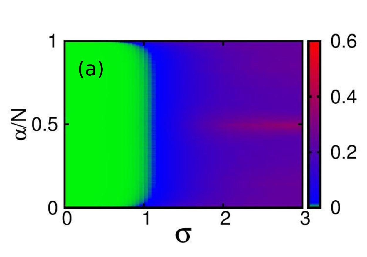
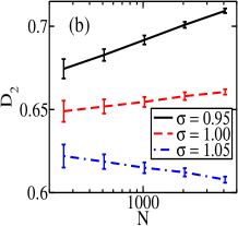
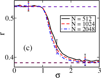
Figure 1: (a) Surface plot of IPR of the single particle eigenstates as a function of $\sigma$ for system size $N=4096$ and $100$ realizations of disorder. Here $\alpha$ stands for index of single particle eigenstates in ascending order of energy. The color ‘green’ lies right at the bottom of the bar legend, and is barely visible due to its very small value ($\sim 1/N$) - it corresponds to the $IPR$ of delocalized eigenstates. (b) Variation of $D_{2}$ with $N$ showing change of slope around $\sigma=1$. (c) The level-spacing ratio $r$ as a function of $\sigma$ for increasing system sizes $N$, averaged over $100$ realizations of disorder. The two dashed horizontal lines denote $r=0.529$ and $r=0.386$ respectively. Error bars are of the same order as the samples shown in the three regions; for other data points, error-bars are suppressed to enhance clarity.

To quantify the point of the localization transition, we compute the inverse participation ratio (IPR), which is defined as

$$I(\alpha)=\sum\limits_{i=1}^{N}{|\psi_{i}(\alpha)|}^{4},$$ (2)

where the coefficients are drawn from the $\alpha^{th}$ normalized single particle eigenfunction $\ket{\psi(\alpha)}=\sum\limits_{i}\psi_{i}(\alpha)\ket{i}$ expanded in the complete set of the Wannier basis $\ket{i}$, which represents the state of a single particle localized at the site $i$ of the lattice. IPR of all the eigenstates as a function of $\sigma$ is shown in the surface plot Fig. 1(a). We see the presence of localized states at the edges of the band near $\sigma=1$, which is essentially a finite size effect Lima et al. (2004).

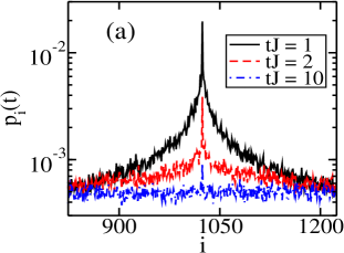
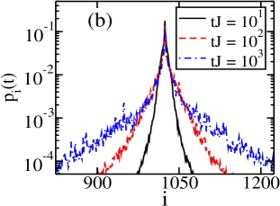
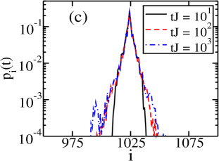
Figure 2: Probability distribution $p_{i}(t)$ for finding a single particle, initially at the middle of the lattice, at each site of the lattice for increasing values of time (in units of $J^{-1}$) (a) for $\sigma=0.5$ (delocalized phase); (b) for $\sigma=1.5$ (quasilocalized phase); and (c) for $\sigma=3.0$ (localized phase) respectively. For all the plots $N=2048$ and number of disorder realizations is $100$.

We also calculate the participation moments averaged over all the eigenstates. The $q^{th}$ participation moment is obtained by averaging over all the eigenstates and disorder configurations

$$P_{q}=\bigg{\langle}\frac{\sum\limits_{\alpha=1}^{N}{P_{q}}(\alpha)}{N}\bigg{\rangle},$$ (3)

where ${P_{q}}(\alpha)=1/\sum\limits_{i=1}^{N}|{\psi_{i}(\alpha)|}^{2q}$. However, $P_{q}\propto N^{D_{q}(q-1)}$. In a fully delocalized (localized) regime $D_{q}$ approaches unity (zero) as the thermodynamic limit is approached. It is evident that $\frac{\log P_{q}}{\log N}\propto D_{q}(q-1)$ and from the variation of $D_{q}$ with the system size, one can identify the point of transition in the thermodynamic limit. We choose $q=2$ and $D_{2}$ is plotted with the system size in Fig.1(b). The $D_{2}$ vs $N$ plot changes slope at $\sigma=1$, which is the point of the localization transition.

The mean of the ratio Oganesyan and Huse (2007); Atas et al. (2013) $r$ between adjacent gaps ($\delta$) in the spectrum can be used to identify a crossover from Wigner-Dyson statistics in the delocalized phase to Poisson statistics in the localized phase. Defining

$$r_{k}=\frac{\min(\delta_{k},\delta_{k+1})}{\max(\delta_{k},\delta_{k+1})},$$ (4)

where $\delta_{k}=\epsilon_{k+1}-\epsilon_{k}$ is the $k^{th}$ energy gap, the mean ratio is $r=\langle\overline{r}\rangle$, where the bar represents an average over the spectrum, and the angular brackets the average over disorder. It is known from random matrix theory that the mean ratio $r$ is approximately $0.529$ in the delocalized phase and $0.386$ in the localized phase Oganesyan and Huse (2007); Atas et al. (2013). Fig. 1(c), based on the finite sizes considered here, suggests that the system is in the ergodic phase in the region $0\leq\sigma\leq 1$. Then $r$ starts decreasing till it reaches the localized phase around $\sigma=2$. The intermediate phase showing intermediate distributions is discussed in the following analysis.

In order to better understand the presence of different phases in the system, we have considered a wavepacket initially localized at the middle site $i_{0}$ of the lattice i.e. $\psi_{i}(t=0)=\delta_{i,i_{0}}$ and calculated the evolution of the spatial distribution of the wavepacket with time. The probability of finding a particle at site $i$ at a given instant $t$ is given by $p_{i}(t)=|\psi_{i}(t)|^{2}$. The spatial dependence of the probability distribution for increasing time is shown in Fig.2. It is to be noted that in the quasilocalized phase (Fig.2(b)), the central part of the wavepacket rapidly drops down to a smaller value, which then barely changes with time whereas the tails of the wavepacket keep spreading with time. In the delocalized phase, the occupancy at the initial site along with all the other sites rapidly decreases and the wavepacket takes the form of a uniform distribution(Fig.2(a)) whereas in the localized phase, the dynamics of the wavepacket is almost absent and it becomes almost exponentially localized (Fig.2(c)). Fig. 2 thus shows that the quasi-localized phase is distinct from both the delocalized and localized phases, and yet carries some character of each of these phases.

III Entanglement in the model

Phase transitions in extended quantum systems are known to be captured by different measures of entanglement Horodecki et al. (2009); Amico et al. (2008); Eisert et al. (2010) such as concurrence, entanglement entropy etc. In the subsequent part of this section, we will calculate the von Neumann entanglement entropy between a suitable subsystem and its complement, both for single particle and many particle states. We will investigate if there is a violation of the ‘area law’ of the entanglement entropy and analyze our results on the basis of the localization transition. We will discuss local particle-number fluctuations and its relation with entanglement entropy in the context of the transition in our model. Also we discuss the ‘entanglement contour’ and ‘fluctuation contour’ in this context.

III.1 Single-particle entanglement

First we discuss single-particle entanglement entropy, which has been argued to be a useful resource for quantum information processing van Enk (2005); Dasenbrook et al. (2016). In order to calculate the entanglement entropy between two subsystems A and B for the normalized single particle states, one writes down a normalized single particle eigenstate in the following way

$$\ket{\psi}=\sum\limits_{i\in A}\psi_{i}{c_{i}}^{\dagger}\ket{0}_{A}\otimes\ket{0}_{B}+\sum\limits_{i\in B}\psi_{i}\ket{0}_{A}\otimes{c_{i}}^{\dagger}\ket{0}_{B},$$ (5)

where $\ket{0}_{A/B}$ is the vacuum state in the subsystem A/B. Then the reduced density matrix $\rho^{sp}_{A}=Tr_{B}(\ket{\psi}\bra{\psi})$ has two eigenvalues $p_{A}=\sum\limits_{i\in A}|\psi_{i}|^{2}$ and $p_{B}=1-p_{A}$Jia et al. (2008)(see Appendix A for more details). The single particle entanglement entropy is then given by

$$S^{sp}_{A}=-p_{A}\ln p_{A}-p_{B}\ln p_{B}.$$ (6)

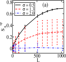
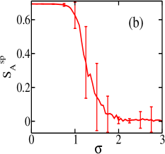
Figure 3: (a) Scaling of single-particle entanglement entropy $S^{sp}_{A}$ with subsystem size $L$ for different values of $\sigma$. (b) Variation of $S^{sp}_{A}$ with $\sigma$, where $L=N/2$. The system size $N=2048$ and number of disorder realizations is $100$ for both the plots.

This entropy is bounded between $\ln 2$ and $0$. In a delocalized eigenstate, $S^{sp}_{A}$ increases with $L$, the size of the subsystem A, as $p_{A}=L/N$ and reaches the maximum value $\ln 2$, when $L=N/2$. In a single site localized state $S^{sp}_{A}$ is $0$ as $p_{A}=1$ or $0$ and does not show any variation with the subsystem size. The variation of $S^{sp}_{A}$ with $L$ in different phases for our model is shown in Fig.3(a). In the quasi-localized phase, $S^{sp}_{A}$ varies with $L$ but its maximum value is less than $\ln 2$ and the maximum value decreases as $\sigma$ increases towards $\sigma=2$. The curves deviate more from the delocalized ones as $L$ increases towards $N/2$ because in the quasilocalized eigenstate the central part of the wavefunction is more localized compared to the tails. The variation of $S^{sp}_{A}$ with $\sigma$ can be seen from Fig.3(b). The delocalized $(\sigma<1)$, quasi-localized $(1<\sigma<2)$ and localized $(\sigma>2)$ phases are clearly seen from the plot. Also it is worth mentioning that the quasilocalized phase shows large intrinsic fluctuations in $S^{sp}_{A}$. This results in large error-bars that cannot be significantly reduced by increasing the number of disorder realizations. This is obvious because in the quasi-localized phase, for an eigenstate, the probability distribution for finding a single particle has multiple peaks and they can appear in random places in the lattice for different realizations of disorder (not shown here) thus making $p_{A}$ a highly fluctuating quantity. In the localized phase the probability distribution is more or less singly peaked hence $p_{A}$ is always close to $0$ or $1$ whereas in the delocalized phase the probability distribution has no peak and it is a uniform one, hence $p_{A}\sim L/N$ giving rise to smaller error-bars in $S^{sp}_{A}$.

III.2 Fermionic entanglement and fluctuations

In this subsection we consider noninteracting spinless fermions at half-filling in the system and investigate signatures of the localization transition via entanglement in many-body states. The connection between localization and entanglement is subtle. Intuitively, one would expect that the greater the delocalization, the more the entanglement and vice versa; however, this correlation is not absolute and counterexamples are availableKannawadi et al. (2016). We also discuss the relationship between subsystem number fluctuations and entanglement entropy in the model. We start with a brief discussion of the calculation of the entanglement entropy of fermions in the ground statePeschel (2003); Peschel and Eisler (2009); Peschel (2012)(see Appendix B for details). For the fermionic many-body ground state $\Ket{\Psi_{0}}$, the density matrix can be written as $\rho=\Ket{\Psi_{0}}\Bra{\Psi_{0}}$. The entanglement entropy between two subsystems is then given by $S_{A}=-Tr(\rho_{A}\log\rho_{A})$, where the reduced density matrix $\rho_{A}=Tr_{B}(\rho)$. However, for a single Slater determinant ground state, Wick’s theorem can be exploited to write the reduced density matrix as $\rho_{A}=\frac{e^{-H_{A}}}{Z}$, where $H_{A}=\sum\limits_{ij}H_{ij}^{A}c_{i}^{\dagger}c_{j}$ is called the entanglement Hamiltonian, and $Z$ is obtained from the condition $Tr(\rho_{A})=1$. The information contained in the reduced density matrix of size $2^{L}\times 2^{L}$ can be captured in terms of the correlation matrix $C$ of size $L\times L$Peschel (2003) within the subsystem A, where $C_{ij}=\left\langle c_{i}^{\dagger}c_{j}\right\rangle$. The correlation matrix and the entanglement Hamiltonian are related byPeschel (2003); Peschel and Eisler (2009); Peschel (2012):

$$C=\frac{1}{e^{H_{A}}+1}.$$ (7)

Using this relation, the entanglement entropy for free fermions is given byPeschel and Eisler (2009); Peschel (2012),

$$S_{A}=-\sum\limits_{m=1}^{L}[\lambda_{m}\log\lambda_{m}+(1-\lambda_{m})\log(1-\lambda_{m})],$$ (8)

where $\lambda_{m}$’s are the eigenvalues of the correlation matrix $C$.

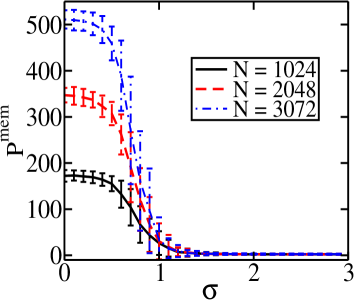
Figure 4: Participation ratio of MEM, denoted as $P^{mem}$, as a function of $\sigma$ for increasing system sizes $N$, averaged over $100$ disorder realizations. Subsystem size $L=N/2$ for fermions at half-filling.

It has been conjectured that the zero mode of the entanglement Hamiltonian has information about topological quantum phase transitions Li and Haldane (2008). The same conjecture can be extended to a non-topological system Pouranvari and Yang (2014). It follows from Eqn. 7 that the zero mode of the entanglement Hamiltonian would correspond to the eigenfunction of the correlation matrix, whose eigenvalue is equal (closest) to $0.5$ . As this eigenmode contributes the maximum to the entanglement entropy, it is called the maximally entangled mode (MEM). The participation ratio of the MEM reflects the localization transition at $\sigma=1$ [Fig. 4]. This is a nice example of detecting the localization transition from the entanglement spectra without having any prior knowledge about the original Hamiltonian.

Now we will discuss the scaling of the entanglement entropy with subsystem size. Typically, short range models of noninteracting fermions show logarithmic violation of the area law of entanglement entropy i.e. $S_{A}\sim L^{d-1}\log L$ in $d$ dimensions Swingle (2010). In our disordered long-range model we see super-logarithmic area law violation in the delocalized phase where $0<\sigma<1$. In fact it goes as $L^{\beta}$, where the exponent $\beta=1$ at $\sigma=0$ and $\beta$ decreases as $\sigma$ increases [Fig. 5](a). In the quasilocalized regime $1<\sigma<2$ it shows area law for larger subsystem sizes whereas in the localized phase $\sigma\geq 2$ it shows a strict area law.

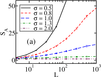
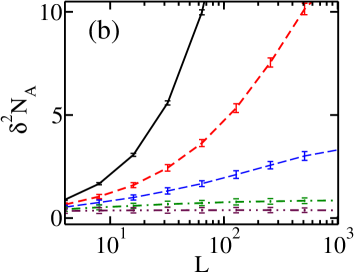
Figure 5: (a) A linear-log plot showing the scaling of the entanglement entropy $S_{A}$ with subsystem size $L$ for increasing $\sigma$ for fermions at half-filling. (b) Similar plot for the number fluctuation $\delta^{2}N_{A}$. For both the plots lattice size $N=2048$ and number of disorder realizations is $100$.

Next we discuss entanglement and its indirect experimental measurement. It has been argued Frérot and Roscilde (2015) that fluctuations of a globally conserved quantity inside a subsystem can measure entanglement entropy as the quantity shares eigenfunctions with the reduced density matrix $\rho_{A}$ and hence provides a good basis for Schmidt decomposition of the many-particle eigenstate (see Ref. Frérot and Roscilde, 2015 for a rigorous proof). In our canonical set-up, total particle number is conserved and we study fluctuations in the particle number inside the subsystem, which is also an experimentally measurable quantityAstrakharchik et al. (2007); Klawunn et al. (2011). The particle number fluctuations inside some subsystem $A$ can be defined as

$$\delta^{2}N_{A}=\sum_{i\in A}\langle n_{i}^{2}\rangle-\langle n_{i}\rangle^{2}.$$ (9)

A close connection exists between entanglement entropy and fluctuations in the local observables in the subsystem e.g. magnetization in a spin system or particle number in free fermionic systemsKlich and Levitov (2009); Song et al. (2010, 2011, 2012); Calabrese et al. (2012); Thomas and Flindt (2015). The relationship becomes a proportionality for certain gapless models, and the proportionality constant to leading order has also been obtained Calabrese et al. (2012).

We adopt this quantity to study our long-ranged model, and look at the scaling of the particle number fluctuations with the subsystem size. The number fluctuations in the subsystem can be calculated using the following relation:

$$\delta^{2}N_{A}=\sum\limits_{m=1}^{L}\lambda_{m}(1-\lambda_{m}).$$ (10)

Fig 5(b) reveals that this quantity shows exactly the same scaling as $S_{A}$, pointing to a proportionality between them, even in this long-range off-critical model. We will see that the proportionality constant offers a signature for the localization-delocalization transition in the model though. Likewise, the proportionality constant shows a sudden jump at the phase transition in the AAH model as well, as will be shown at the end of this section.

III.3 Entanglement contour and fluctuation contour

In this subsection, we will define and study the ‘entanglement contour’Chen and Vidal (2014) and the ‘fluctuation contour’Frérot and Roscilde (2015). These quantities contain microscopic details of entanglement and number fluctuations. Specifically, the contour keeps track of the contribution from each site within the subsystem, to the quantity under consideration. Entanglement contour is defined as the contribution ($C_{s}(i)\geq 0$) from the degrees of freedom at each site $i$ in subsystem A to the entanglement entropy $S_{A}$ such that $S_{A}=\sum\limits_{i\in A}C_{s}(i)$. One can calculate $C_{s}(i)$ using the following relationChen and Vidal (2014):

$$C_{s}(i)=\sum\limits_{m=1}^{L}g_{i}(m)S_{m},$$ (11)

where $S_{m}=-[\lambda_{m}\log\lambda_{m}+(1-\lambda_{m})\log(1-\lambda_{m})]$. Here $\lambda_{m}$’s are the eigenvalues of the correlation matrix $C$ or the entanglement spectra. $g_{i}(m)$ describes the spatial pattern of the $m^{th}$ normalized eigenstate $\ket{\phi(m)}$ of matrix $C$ and hence of the entanglement Hamiltonian $H_{A}$ i.e. $g_{i}(m)=|\phi_{i}(m)|^{2}$. Similarly, one can define the contour of subsystem particle-number fluctuations (also called as ‘fluctuation contour’) $C_{n}(i)=\langle\delta n_{i}\delta N_{A}\rangle$, which is an obvious decomposition of the particle-number fluctuations ($\delta^{2}N_{A}$) in $A$ such that $\delta^{2}N_{A}=\sum\limits_{i\in A}C_{n}(i)$. In the canonical ensemble $\delta N_{A}=-\delta N_{B}$. Then $C_{n}(i)=-\langle\delta n_{i}\delta N_{B}\rangle$. So one can interpret $C_{n}(i)$ as the correlation between number (density) fluctuations at site $i$ and those in the whole of subsystem $B$. It can also be defined asFrérot and Roscilde (2015)

$$C_{n}(i)=\sum\limits_{m=1}^{L}g_{i}(m)\lambda_{m}(1-\lambda_{m}),$$ (12)

where all the terms have the same meaning as defined previously.

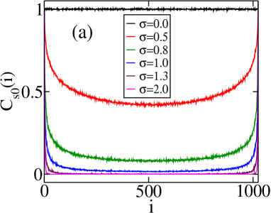
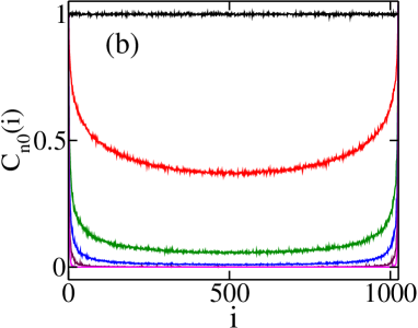
Figure 6: (a) Spatial distribution of the scaled entanglement contour $C_{s0}(i)$ in the subsystem for different $\sigma$. (b) The same for the fluctuation contour $C_{n0}(i)$ for increasing values of $\sigma$. For all the plots $N=2048$ and number of disorder realizations is $100$. Here $i$ is the site index in the subsystem and subsystem size $L=N/2$ for half-filled fermions.

It turns out that for free fermionic systems $C_{n}(i)$ and $C_{s}(i)$ show similar spatial dependence Frérot and Roscilde (2015). Spatial dependence of the $C_{s0}(i)=C_{s}(i)/C_{s}(1)$ entanglement contour and the scaled fluctuation contour $C_{n0}(i)=C_{n}(i)/C_{n}(1)$ of the random long-range hopping model are shown in Fig.6(a) and in Fig.6(b) respectively. Since there are two boundaries between two subsystems in a ring and because the entanglement and the number fluctuations decay as one moves away from the boundaries, contours are symmetric functions of sites with respect to the midpoint of subsystem $A$. We fit this decay with the function $1/x^{\gamma}$. Since the entanglement entropy is the sum of all the contributions of the entanglement contour, one may guess that the entanglement entropy dependence should be given by the integral $\int\frac{1}{x^{\gamma}}dx$, which in turn suggests that the exponent $\beta$ should be given by $\beta\approx 1-\gamma$. Indeed, we find evidence for this[Fig. 7], deep in the delocalized phase.

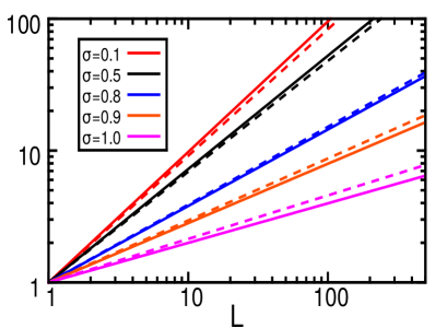
Figure 7: The exponent $\beta$ calculated from the subsystem scaling of the entanglement entropy and the other exponent $\gamma$ determined from the decay of the entanglement contour in the subsystem are compared. In this log-log plot $L^{\beta}$ (solid lines) and $L^{1-\gamma}$ (dashed lines) are plotted to establish the relation $\beta\approx 1-\gamma$ in the delocalized phase $\sigma<1$.

For a finer understanding of the entanglement contour at the boundaries and in the bulk of the subsystem, the histogram of $C_{s}(i)$ is plotted in Fig.8. In the delocalized regime, the entanglement contour has a finite value at all the sites and the histogram is a sharply peaked distribution whereas the distribution gets broadened and the peak shifts towards $0$ as one approaches the point of quasi-localization $\sigma=1$ [Fig.8(a)]. In the quasilocalized regime the entanglement contour deep in the bulk starts vanishing [Fig.8(b)], which explains the validity of the area law for larger subsystem size. In the localized regime the entanglement contour almost vanishes in the whole bulk region and one gets a strict area law in this regime. This is also evident from the histogram for $\sigma=2.0$ in Fig.8(b) which shows a sharp peak at $0$ with almost no broadening.

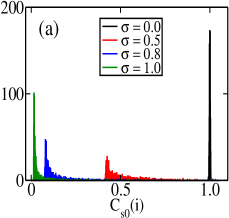
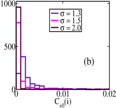
Figure 8: Histogram of the scaled entanglement contour $C_{s0}(i)$ (a) in the delocalized phase ($\sigma<1$); (b) in (quasi)localized phase ($\sigma>1$) respectively. For both the plots spinless fermions at half-filling are considered in a system of size $N=2048$. Here i indicates sites in the subsystem, whose size $L=N/2$ and number of disorder realizations is $100$.

The fluctuation contour also shows similar behavior as the entanglement contour (not shown here).

Since the entanglement entropy and local number fluctuations are intimately related, it is useful to study this relationship at a microscopic level by calculating the ratio of the two contours of the related quantities i.e. $K(i)=C_{s}(i)/C_{n}(i)$. This ratio for increasing values of $\sigma$ in the delocalized phase is shown in Fig.9(a). It reveals a uniform proportionality between the two contours in the deep delocalized regime. The proportionality becomes non-uniform as $\sigma$ approaches the transition point $\sigma_{c}=1$. In the (quasi)localized regime this non-uniformity becomes so much worse that we omit these data in the interest of clarity. A histogram in Fig.9(b) shows a peaked distribution of $K(i)$ for smaller $\sigma$ and the distribution gets broadened with almost vanishing peak for larger $\sigma$.

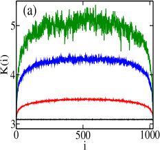
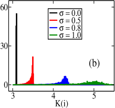
Figure 9: (a) Spatial distribution of the ratio of two kinds of contour $K(i)$ of half-filled fermions for increasing $\sigma$ in the delocalized phase. (b) The corresponding histogram of $K(i)$. Here lattice size $N=2048$ and $i$ is the site index within subsystem $L=N/2$ and number of disorder realizations is $100$.

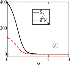
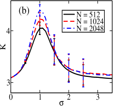
Figure 10: (a) Variation of the entanglement entropy $S_{A}$ and number fluctuation in the subsystem $\delta^{2}N_{A}$ of half-filled fermions with $\sigma$. Here the system size $N=2048$. (b) The ratio of the two quantities $K$ as a function of $\sigma$ for different system sizes $N$. In both the plots subsystem size $L=N/2$ and number of disorder realizations is $100$.

Next we study the proportionality constant $K$ of the relationship $S_{A}=K\delta^{2}N_{A}$ for free fermionic models. In a gapless system, $S_{A}\propto\log L$ and $K=\pi^{2}/3$ for a 1D Fermi gas as shown in a recent articleCalabrese et al. (2012). However, in a gapped system $K$ is not known in general; furthermore, $K$ is not believed to be a universal quantity. This motivates us to investigate $K$ in our long-range model. Though entanglement entropy and number fluctuations in the subsystem vary in a similar fashion with $\sigma$ [Fig.10(a)], near the transition they conspire in such a way that the ratio of them leaves a signature for the transition in the model [Fig.10(b)]. The proportionality constant $K$ shows a maximum at $\sigma_{c}=1$ and becomes almost constant in the localized phase $(\sigma>2)$. Large error bars in the (quasi)localized regime in Fig.10(b) are a reflection of the largely broadened distribution of $K(i)$ in the same regime.

III.4 Comparison with AAH model

In the following, we have done a similar study as above in the AAH model which is a short-range model that shows a sharp localization-delocalization transition at finite disorder.

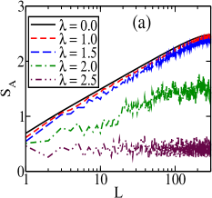
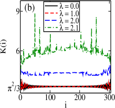
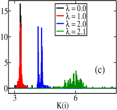
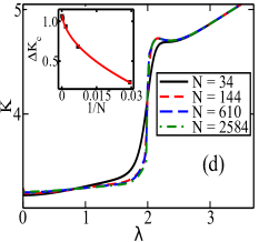
Figure 11: Results from the 1D AAH model. (a) Scaling of the entanglement entropy $S_{A}$ with the subsystem size $L$ for increasing $\lambda$. The x axis is plotted in log-scale. (b) The ratio of entanglement contour to fluctuation contour $K(i)$ in the subsystem for different $\lambda$. (c) The corresponding histogram of $K(i)$. For the plots((a)-(c) $N=610$ (d) Proportionality constant $K$ as a function of $\lambda$ for increasing $N$. The inset is a fit to the $\Delta K_{c}$ vs $1/N$ data points(black square), where $\Delta K_{c}=K(\lambda=2.025)-K(\lambda=1.975)$. The red curve represents the fitting curve given by $\Delta K_{c}=1.12-5.47/N^{0.51}$. For all the plots, the subsystem size $L=N/2$ (except for figure (a)) for fermions at half-filling.

The AAH model can be described by a Hamiltonian of the same form as Eqn.1 where $t_{ij}=\delta_{i,j+1}$ and $v_{i}=\lambda\cos(2\pi\eta i)$. Here $\eta$ is a ‘Diophantine number’ (e.g. $\frac{\sqrt{5}-1}{2}$, inverse of the ‘golden mean’) and $\lambda$ is the strength of the quasi-periodic disorderAubry and André (1980); Harper (1955). All the single particle eigenstates get localized at $\lambda_{c}=2$Jitomirskaya (1999).

Our results for the Harper model are summarized in Fig.11. In the tight binding model without any disorder $S_{A}\sim\log L$. As the quasi-periodic disorder is turned on, in the delocalized phase ($\lambda<2$) $S_{A}$ retains the factor of $\log L$ which is a modulated area-law behavior and in the localized phase ($\lambda\geq 2$) $S_{A}$ shows a strict area law, as shown in Fig.11(a). In the delocalized regime $K(i)$ is close to $\pi^{2}/3$ in the bulk whereas as one enters the localized regime it is no more a constant and starts fluctuating [Fig.11(b)]. This is also evident from the histogram of the same quantity. The distribution gets broadened and the peak almost disappears in the localized phase Fig.11(c). Also $K$ shows a jump at the transition point $\lambda_{c}=2$ [Fig.11(d)]. We define $\Delta K_{c}=K_{\lambda=2+\delta\lambda}-K_{\lambda=2-\delta\lambda}$ near the quantum critical point $\lambda_{c}=2$, the scaling of which with the system size $N$ is well fitted by the functional form $\Delta K_{c}=1.12-5.47/N^{0.51}$ for $\delta\lambda=0.025$ (the inset of Fig.11(d)). As $N\rightarrow\infty$, $\Delta K_{c}=1.12$. So when $\delta\lambda\rightarrow 0$, $dK/d\lambda$ will diverge to $\infty$ at $\lambda_{c}=2$ and hence the $K$ vs $\lambda$ plot will become vertical at $\lambda_{c}=2$ in the thermodynamic limit. The proportionality constant $K$ indeed captures transitions in the system although it changes differently in the two models studied here.

IV Non-equilibrium dynamics

Having studied the static quantities to analyze different phases, in this section we investigate the dynamical properties of the model. A non-equilibrium situation can be created by changing a parameter of the Hamiltonian, locally or globally, through adiabatic or sudden processes. Here we study the dynamics of entanglement entropy post a sudden global quench in the bond-disordered long-range model and compare the results with those of charge transport in the system. We also briefly discuss correlation transport in the system in the context of velocity bounds on transport and the related light-cone picture Lieb and Robinson (1972). We calculate the growth of bipartite entanglement entropy $S_{A}(t)=-Tr(\rho_{A}(t)\ln(\rho_{A}(t)))$, between two halves of the system A and B for our model at half-filling. The data we present are with an initial state of the density-wave(DW) type $\ket{\Psi}=\prod\limits_{i}{c_{2i}}^{\dagger}\ket{0}$, which is evolved under the Hamiltonian at a particular $\sigma$Chiara et al. (2006). The DW state can be achieved by turning on an additional strong repulsive nearest neighbor interaction and then suddenly turning it off. We have checked that qualitatively similar results are obtained when the initial state is the many-body ground state of half-filled fermions corresponding to the Hamiltonian at $\sigma=2.5$, with a quench carried out to various other values of $\sigma$. To calculate entanglement entropy, we use standard free fermion techniques Peschel (2003); Chiara et al. (2006)(see Appendix C for details). Variation of $S_{A}(t)$ with time for the DW type of initial state is shown in Fig.12(a). The entanglement entropy varies with time in faster-than-linear fashion for $\sigma<1$ before it saturates, indicating the existence of a non-equilibrium steady state. In the (quasi)localized regime ($\sigma>1$), after a super-ballistic transient $S_{A}(t)$ goes in a sub-linear fashion with time before reaching a saturating steady state. In the delocalized phase, the saturation value $S_{A}^{\infty}$ barely changes with $\sigma$; however in the quasi-localized phase, $S_{A}^{\infty}$ decreases with increasing $\sigma$. In the localized phase ($\sigma>2$) the entanglement growth becomes substantially suppressed as compared to the corresponding translationally invariant nearest neighbor model Calabrese and Cardy (2005), where the entanglement entropy reaches the saturation at a time $t_{sat}\sim L/2$. Also the saturation values of $S_{A}$ in the localized phase are negligibly small. The number fluctuations $\delta^{2}N_{A}$, which are essentially density-density correlations, reveal similar dynamics as $S_{A}(t)$ [Fig.12(b)].

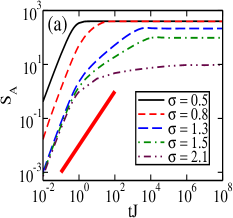
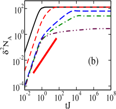
Figure 12: (a) Quench dynamics of the entanglement entropy $S_{A}$ of half-filled fermions with time (in units of $J^{-1}$) for increasing $\sigma$ from an initial DW type state. (b) Similar plot for subsystem number fluctuations $\delta^{2}N_{A}$. For both the log-log plots $N=2048$, $L=N/2$ and number of disorder realizations is $100$. The thick line segment shows linear dependence on time for comparison.

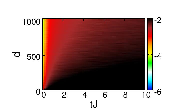
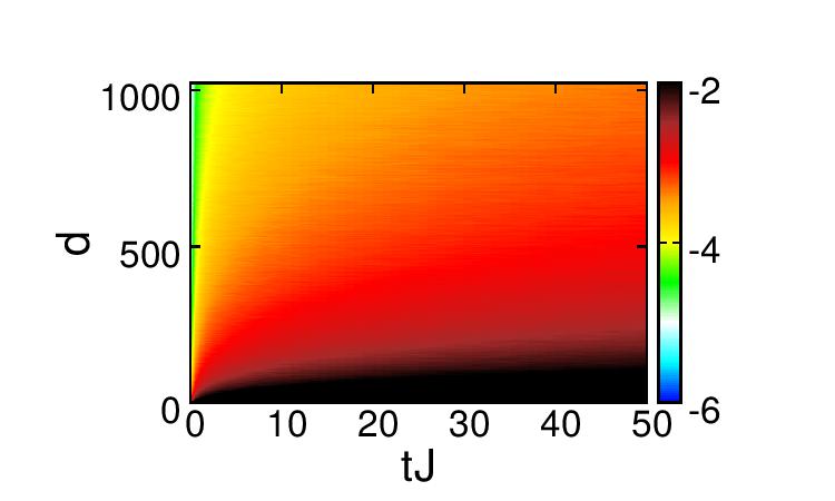
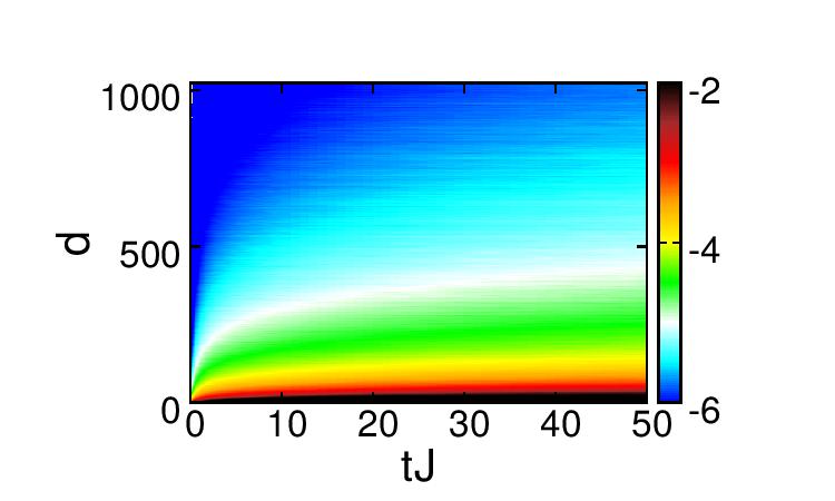
(a) (b) (c)

Figure 13: (a)-(c) Surface plot showing the spreading of the amount of correlation $\log_{10}|C_{d}(t)|$ in time (in units of $J^{-1}$) and the lattice distance $d$ for $\sigma=0.8,1.3,2.1$ respectively. Here $d=|i-j|$, is the lattice distance between sites $i$ and $j$. The colors represent different ranges of values of the correlation, indicated in the bar legend attached to each figure - the numbers mentioned in the bar legend are the powers to be which ten is raised. For all the plots half-filled fermions are studied with $N=2048$, $L=N/2$ and number of disorder realizations is $100$. The initial state is the DW state, described in the text.

In short-range models with translational invariance, following a global quench correlation transport happens with a constant velocity, defined as the Lieb-Robinson boundLieb and Robinson (1972), giving rise to a sharp causal light-cone like view of the correlation transport in space-time, outside of which correlations are exponentially suppressedCalabrese and Cardy (2006). This leads to linear growth of entanglement entropy in such modelsCalabrese and Cardy (2005). Breaking of translation invariance in short-range models can give rise to a much slower light cone, e.g. a logarithmic light-cone in the Anderson-localized phaseBurrell et al. (2009) and hence the entanglement entropy also shows a slow growth. More than a linear growth of the entanglement entropy with time indicates the violation of the picture based on Lieb-Robinson bounds, which also bound the rate of growth of the entanglement. This kind of violation has actually been seen very recently in ultracold ionic experiments with translationally invariant long-range interacting spin modelsRicherme et al. (2014); Jurcevic et al. (2014). Also theoretical investigations have been carried out for translationally invariant long-range free fermionic models in this contextStorch et al. (2015); Buyskikh et al. (2016); Van Regemortel et al. (2016). To test the validity of the light-cone picture for correlation transport in our long-range free fermionic model with disordered hopping, we calculate the two-point correlation function $C_{d}=\langle{c_{i}}^{\dagger}c_{j}\rangle$ as function of time ($tJ$) and distance ($d=|i-j|$) between the sites $i$ and $j$ inside the subsystem as depicted in the surface plot in Fig. 13. At time $tJ=0$ the correlation matrix is diagonal with zero off-diagonal elements due to the product state structure of the initial DW state and the entanglement entropy is zero. At later times, different sites at distance $d=|i-j|$ start getting correlated. The correlation transport is more than linear or super-ballistic in nature within very short time-scales $tJ\sim 1$, which shows up as a transient in the quasi-localized $(1<\sigma<2)$ and localized $(\sigma>2)$ phases whereas in the delocalized phase, super-ballistic part is predominant as the time-scale for entanglement growth till it reaches the saturation is shorter ($t_{sat}J\sim 1$) in this case. This explains the super-ballistic entanglement growth in the system and violation of the picture based on Lieb-Robinson bounds. However later time dynamics of the correlation reveals different behaviors of the light-cone picture in three different phases as we detail it in the following. As we can see from Fig. 13(a) for $\sigma=0.8$, one can still perceive sub-linear light-cones in the delocalized regime. Sub-linearity indicates a decreasing velocity of the correlation transport with time as opposed to a constant velocity in the linear light-cone picture. The light-cone becomes more prominent and more sub-linear in the quasi-localized regime as can be seen in Fig.13(b). Very sharp sub-linear light-cones are visible in the localized regime (Fig.13(c)), where velocities of the correlation transport depend on the threshold values of the correlation. Sub-linearity of light-cones is more in this regime and hence the growth of entanglement entropy is very slow in the same regime. Such a change in light-cone picture from less prominent to more prominent can be seen in the three regimes $(\sigma<1,1<\sigma<2$ and $\sigma>2)$ also for the corresponding translationally invariant long-range hopping model with initial DW stateStorch et al. (2015). In contrast to our model though, in the non-disordered model, all the light cones look linear and the related velocity bounds on the correlation transport decrease as $\sigma$ decreases.

Next we will compare entanglement transport with charge transport in the system at the single-particle and many-particle levels. Single-particle entanglement entropy $S^{sp}_{A}$ is calculated by choosing the subsystem $A$ such that it continues to be half the size of the total system, but it is now taken to be centered around the initial localized wavepacket in the middle of the lattice. The dynamics of $S^{sp}_{A}$ reveals super-ballistic nature in the delocalized phase but in the (quasi)localized phase the initial super-ballistic behavior is followed by a ballistic part before saturation [Fig. 14(a)]. Also the average width of the initially localized wavepacket is calculated, which is defined as

$$w^{sp}(t)=\sqrt{\sum\limits_{i}(i-i_{0})^{2}p_{i}(t)},$$ (13)

where $p_{i}(t)=|\psi_{i}(t)|^{2}$ as also mentioned earlier and $i_{0}$ is the center of the lattice. The dynamics of the width in different phases is shown in Fig.14(b). In the (quasi)localized phase, after a ballistic transient, $w^{sp}(t)$ goes sub-linearly before it reaches a saturation value and the exponent of the sub-linear variation decreases as $\sigma$ increases. This signals a sharp contrast between charge transport and entanglement dynamics even within the single-particle picture. Although both the quantities reach saturation at the same time, the saturation values decrease abruptly with $\sigma$ in the quasi-localized phase and becomes vanishingly small in the localized phase.

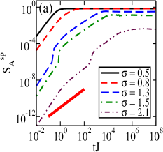
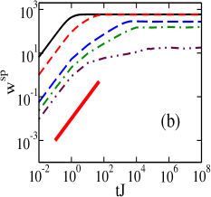
Figure 14: (a) The single-particle entropy $S^{sp}_{A}$ as a function of time (in units of $J^{-1}$) for increasing $\sigma$. (b) Similar plot for the width $w^{sp}$ of the single particle wavepacket. The thick solid line shows the linear dependence on time for comparison. For all the log-log plots $N=2048$, $L=N/2$ and number of disorder realizations is $100$.

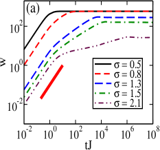
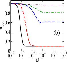
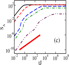
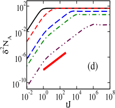
Figure 15: (a)-(b) Variation of width $w$ of the many-particle wavepacket and the occupation density of the initially occupied sites $n_{loc}$ respectively with time (in units of $J^{-1}$) for increasing $\sigma$. In the delocalized phase $n_{loc}$ is just the filling fraction in the long-time limit. (c)-(d) Variation of the entanglement entropy $S_{A}$ and number fluctuations in the subsystem $\delta^{2}N_{A}$ respectively with time(in units of $J^{-1}$) for increasing $\sigma$. The thick solid line shows linear dependence on time for comparison. For all the log-log plots $N=2048$, $L=N/2$ and number of disorder realizations is $100$ for fermions with filling fraction $0.1$ .

We also study the expansion dynamics of a cloud of fermions of a given filling and initial state in which fermions sit around the center of the lattice. This type of initial state can be prepared by switching on a trap potential and suddenly switching it off to study the evolution of the system under the quenched Hamiltonian. We calculate the expansion of the width of the many-particle cloud, which can be quantified bySchneider et al. (2012)

$$w(t)=\sqrt{\frac{1}{N_{p}}\sum\limits_{i}(i-i_{0})^{2}\langle n_{i}(t)\rangle-\frac{1}{N_{p}}\sum\limits_{i}(i-i_{0})^{2}\langle n_{i}(0)\rangle},$$ (14)

where $N_{p}$ is the total number of particles and $\langle n_{i}\rangle$ is the average occupation at site $i$ whereas $i_{0}$ is the center of the lattice. Simultaneously another quantity $n_{loc}$, which is the sum of the occupation densities at the initially occupied sites, is also investigated as a function of time. This quantity is defined asRibeiro et al. (2013):

$$n_{loc}(t)=\frac{1}{N_{p}}\sum\limits_{i}^{in.occ.}\langle n_{i}(t)\rangle.$$ (15)

The width of the many-particle wavepacket $w$ in different phases is shown in Fig.15(a) and it shows the same qualitative feature as $w^{sp}$. The variation of $n_{loc}$ with time nicely matches with the dynamics of $w$ [Fig.15(b)]. It decreases rapidly to the saturation value, which is filling fraction in the delocalized phase and barely changes in the localized phase. In the quasi-localized phase, it saturates to an intermediate value, which increases abruptly as $\sigma$ increases in the same phase. Also we calculate the entanglement entropy for the same initially localized many-particle state by choosing a subsystem of $L=\frac{N}{2}$ consecutive sites, whose center coincides with the center of the lattice. It shows the same qualitative feature as $S^{sp}_{A}$[compare Fig. 14(a) and Fig.15(c)]. Therefore, similar to the single-particle picture, there is a contrast between charge transport and entanglement propagation in the many-particle picture. The number fluctuations also show similar dependence on time but it is smoother than $S_{A}$ [Fig.15(d)]. The roughness of $S_{A}$ and $S^{sp}_{A}$ may be an artifact to the special choice of the subsystem. This whole analysis has been carried out at a filling of $0.1$; however, we have verified that there is no qualitative dependence of these results on the filling fraction since there is no mobility edge in the energy spectra.

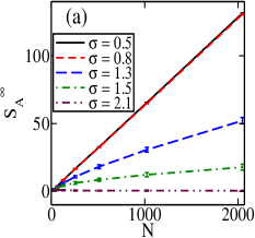
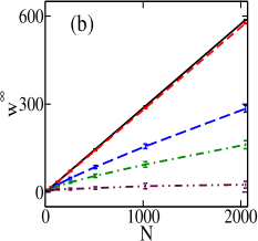
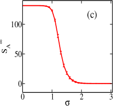
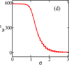
Figure 16: (a)-(b) Scaling of the saturation values of the entanglement entropy $S_{A}^{\infty}$ and width of the many-particle wave-packet $w^{\infty}$ respectively with the system size $N$. (c)-(d) Variation of $S_{A}^{\infty}$ and $w^{\infty}$ respectively with $\sigma$. For Fig.(c),(d) $N=2048$. For all the plots $L=N/2$ and number of disorder realizations is $100$ for fermions with filling fraction $0.1$ .

The saturation values of the many-particle entanglement entropy and the width of the wavepacket show similar variation with the system sizes $N$ [Fig.16(a-b)]. In the delocalized phase both the quantities go linearly with $N$ whereas in the quasi-localized phase the dependence is sub-linear and they become almost independent of $N$ in the localized phase. This is quite expected as it reflects the sensitivity of the three phases to the boundaries of the system. The variation of these two quantities with $\sigma$ is shown in [Fig.16(c-d)] and they show similar dependences. In the delocalized phase both the quantities have almost constant and very high values whereas in the quasi-localized phase their values decrease abruptly with $\sigma$ and for large $\sigma$ in the localized phase, become tiny and almost $\sigma$-independent.

V Conclusion

To summarize, in this paper we study many static and dynamical quantities to investigate the link between the delocalization-localization transition and entanglement of spinless fermions in a random long-range hopping model. Within the system sizes used for numerical analysis, the system shows a delocalized phase for $\sigma<1$ and a localized phase for $\sigma>2$. One also obtains a quasi-localized phase for $1<\sigma<2$, as reflected by the level-spacing ratio and wave-packet dynamics, but this phase may vanish in the thermodynamic limit as hinted in the plots of level-spacing ratio for different system sizes. Scaling of the entanglement entropy with subsystem size reveals strong area-law violation in the delocalized phase whereas the (quasi)localized phase seems to adhere (for larger subsystems) strictly to the area law. In addition to the eigenvalues of the entanglement Hamiltonian, the maximally entangled mode or the zero mode of the entanglement Hamiltonian, also captures the localization transition, despite it being a non-topological system. The entanglement contour, which is constructed out of both the eigenvalues and the eigenfunctions of the entanglement Hamiltonian, gives a picture of the spatial distribution of entanglement inside the subsystem and nicely explains the violation of the area-law in the system. Particle-number fluctuations in the subsystem have similar dependence on space and time as the entanglement entropy. The ratio of these two quantities shows a sharp signature at the point of the localization transition. However, the nature of this signature is dependent on the model in question as it is different in the AAH model from our long-range model. The distribution of the ratio of the entanglement contour to the fluctuation contour is sharply peaked in the delocalized phase but the peak starts vanishing as one goes into the (quasi)localized phase.

Also we study quench dynamics and wave-packet dynamics of fermions at the single-particle and many-particle levels. At both the levels the entanglement propagation and the charge transport show a sharp contrast. Entanglement entropy shows super-ballistic behavior both in the delocalized phase and the (quasi)localized phase, although this appears only as a transient in the latter. This super-ballistic behavior is attributed to the picture based on the Lieb-Robinson bounds for the spreading of correlation post a global quench. Contrastingly, the width of the wave-packet varies ballistically with time in the delocalized phase while in the (quasi)localized phase after ballistic transient it shows a sub-ballistic behavior with time before it saturates. In a short-range model with disorder, the light cone picture is valid, and therefore the time dependence of entanglement entropy is always sub-ballistic in general. However, in our model long-range couplings give rise to super-ballistic behavior. The saturation values of the width and entanglement entropy show similar dependence as a function of the system size and $\sigma$ reflecting the presence of three phases in finite systems.

In our study, we have been able to explain the strong area law violation in our long-range model by implementing the idea of entanglement contour and connect them to the delocalization-localization transition in the system by studying quench and wave-packet dynamics. We hope that our results regarding the relationship between entanglement entropy and number fluctuations will help boost the possibility of indirect measurement of entanglement in experiments. Also we have shown explicitly the contrast between charge and entanglement transport, which is one of the current topics of interest. As a future possibility, one can also look for many-body localized phases in an interacting version of this model. We hope that our work can trigger experimental studies of the disordered long-range model in ongoing ionic trap experiments.

Appendix

Here we provide a detailed discussion about the methodologies used in the paper to calculate, namely, the single particle entanglement entropy, the fermionic entanglement entropy and non-equilibrium dynamics of the entanglement entropy.

Appendix A Single particle Entanglement Entropy

A normalized single particle eigenstate $\ket{\psi}$ can be expressed as,

$$\ket{\psi}=\sum\limits_{i\in A}\psi_{i}{c_{i}}^{\dagger}\ket{0}_{A}\otimes\ket{0}_{B}+\sum\limits_{i\in B}\psi_{i}\ket{0}_{A}\otimes{c_{i}}^{\dagger}\ket{0}_{B},$$ (16)

where $\ket{0}_{A}=\underset{i\in{A}}{\otimes}\Ket{0}_{i}$ and $\ket{0}_{B}=\underset{i\in{B}}{\otimes}\Ket{0}_{i}$.

We define $\ket{1}_{A}=\frac{1}{\sqrt{p_{A}}}\sum\limits_{i\in{A}}\psi_{i}{c_{i}}^{\dagger}\ket{0}_{A}$ and $\ket{1}_{B}=\frac{1}{\sqrt{p_{B}}}\sum\limits_{i\in{B}}\psi_{i}{c_{i}}^{\dagger}\ket{0}_{B}$.

Here $p_{A}=\sum\limits_{i\in A}|\psi_{i}|^{2}$; $p_{B}=\sum\limits_{i\in B}|\psi_{i}|^{2}$ and $p_{A}+p_{B}=1$.

Notice that ${\langle 0|0\rangle}_{A}={\langle 0|0\rangle}_{B}=1$ and ${\langle 1|1\rangle}_{A}={\langle 1|1\rangle}_{B}=1$.

We can now write Eq.16 as,

$$\ket{\psi}=\sqrt{p_{A}}\ket{1}_{A}\otimes\ket{0}_{B}+\sqrt{p_{B}}\ket{0}_{A}\otimes\ket{1}_{B},$$ (17)

The density matrix of the full system $\rho^{sp}=\ket{\psi}\bra{\psi}$.

The reduced density matrix of subsystem A $\rho^{sp}_{A}=Tr_{B}[{\rho^{sp}}]$, which is given by,

$$\rho^{sp}_{A}=p_{A}\ket{1}_{A}\bra{1}_{A}+p_{B}\ket{0}_{A}\bra{0}_{A},$$ (18)

Single particle entanglement entropy $S^{sp}_{A}=-Tr[\rho^{sp}_{A}\ln(\rho^{sp}_{A})]$, which can be written as,

$$S^{sp}_{A}=-{p_{A}}\ln{p_{A}}-{p_{B}}\ln{p_{B}}.$$ (19)

Appendix B Fermionic Entanglement Entropy

In the following, we explain the methodology to calculate entanglement entropy of $N_{p}$ non-interacting spinless fermions in the ground state of a 1D lattice of $N$ sites under periodic boundary condition. The generic Hamiltonian is given by,

$$H_{1}=\sum\limits_{i,j=1}^{N}t_{ij}c_{i}^{\dagger}c_{j}+h.c.$$ (20)

The diagonal form of the Hamiltonian is given by,

$$H_{1}=\sum\limits_{k=1}^{N}\epsilon_{k}b_{k}^{\dagger}b_{k},$$ (21)

where $b_{k}=\sum\limits_{j=1}^{N}\psi_{j}(k)c_{j}$.
We calculate the entanglement entropy for the fermionic ground state, which is defined as,

$$\ket{\Psi_{0}}=\prod_{k=1}^{N_{p}}b_{k}^{\dagger}\ket{0}$$ (22)

Due to Slater determinant structure of $\ket{\Psi_{0}}$, all higher correlations can be obtained by two point correlation $C_{ij}=\langle c_{i}^{\dagger}c_{j}\rangle$Peschel (2003); Peschel and Eisler (2009); Peschel (2012). The density matrix of the full system $\rho=\ket{\Psi_{0}}\bra{\Psi_{0}}$ and the reduced density matrix of subsystem A $\rho_{A}=Tr_{B}(\rho)$. By definition a one particle function, in this case two-point correlation in the subsystem, can be written as,

$$C_{ij}=Tr[\rho_{A}c_{i}^{\dagger}c_{j}]$$ (23)

However, this is possible according to Wick’s theorem only when the reduced density matrix is the exponential of free fermionic operatorPeschel (2003),

$$\rho_{A}=\frac{e^{-H_{A}}}{Z},$$ (24)

where $H_{A}=\sum\limits_{i,j=1}^{L}H_{ij}^{A}c_{i}^{\dagger}c_{j}$ is called the entanglement Hamiltonian, and $Z$ is obtained to satisfy the condition $Tr[\rho_{A}]=1$.
The entanglement Hamiltonian can be written in the diagonal form as,

$$H_{A}=\sum\limits_{k=1}^{L}h_{k}a_{k}^{\dagger}a_{k},$$ (25)

where $a_{k}=\sum_{j=1}^{L}\phi_{j}(k)c_{j}$. The reduced density matrix is then given by,

$$\rho_{A}=\frac{exp[-\sum\limits_{k=1}^{L}h_{k}a_{k}^{\dagger}a_{k}]}{\prod\limits_{k=1}^{L}[1+exp(-h_{k})].}$$ (26)

Using Eq.26, we can write Eq.23 as,

$$C_{ij}=\sum\limits_{k=1}^{L}\phi^{\ast}_{i}(k){\phi}_{j}(k)\frac{1}{e^{h_{k}}+1}.$$ (27)

This shows the matrices $C$ and $H_{A}$ share the eigenstate $\ket{\phi_{k}}$ and their eigenvalues are related by,

$$\lambda_{k}=\frac{1}{e^{h_{k}}+1},$$ (28)

where $\lambda_{k}$’s are eigenvalues of matrix $C$ in the subsystem.
The entanglement entropy $S_{A}=-Tr[\rho_{A}\ln(\rho_{A})]$, which can be simplified Sharma and Rabani (2015) using Eq.26 and Eq.28 as,

$$S_{A}=-\sum\limits_{k=1}^{L}[\lambda_{k}\log\lambda_{k}+(1-\lambda_{k})\log(1-\lambda_{k})],$$ (29)

Appendix C Non-equilibrium dynamics of fermionic Entanglement Entropy

In this section we discuss how to calculate dynamics of fermionic Entanglement entropy in our model, under the Hamiltonian,$H_{1}$ and an initial many-particle state $\ket{\Psi_{in}}$, which is not the many-particle ground state of $H_{1}$. The Hamiltonian is given by,

$$\mathcal{H}=\sum\limits_{i\neq j}^{N}t_{ij}c_{i}^{\dagger}c_{j}+h.c.,$$ (30)

The Hamiltonian can be written in the diagonal form, which is given by,

$$\mathcal{H}=\sum\limits_{k=1}^{N}\epsilon_{k}b_{k}^{\dagger}b_{k},$$ (31)

where $b_{k}=\sum\limits_{j=1}^{N}\psi_{j}(k)c_{j}$. Assuming $\hbar=1$, the time evolution of the Heisenberg operators $b_{k}(t)$ is given by,

$$\dot{b}_{k} =\frac{1}{i}[b_{k},\mathcal{H}]$$

$$=\frac{1}{i}\epsilon_{k}b_{k},$$ (32)

Hence, $b_{k}(t)=e^{-i\epsilon_{k}t}b_{k}(0)$.
Here, for example, we consider a density-wave(DW) type of initial state, defined as,

$$\ket{\Psi_{in}}=c_{2}^{\dagger}c_{4}^{\dagger}....c_{N}^{\dagger}\ket{0},$$ (33)

where lattice sites $N$ is even and number of fermions $N_{p}=N/2$.
In order to calculate the dynamics of the entanglement entropy one first constructs $L\times L$ correlation matrix within the subsystem A or B, i.e. $C_{ij}(t)=\bra{\Psi_{in}}c_{i}^{\dagger}(t)c_{j}(t)\ket{\Psi_{in}}$, where $i,j\in A$. Below we detail the the calculation of $\bra{\Psi_{in}}c_{i}^{\dagger}(t)c_{j}(t)\ket{\Psi_{in}}$.

$$\bra{\Psi_{in}}c_{i}^{\dagger}(t)c_{j}(t)\ket{\Psi_{in}} =\sum\limits_{k,k^{\prime}=1}^{N}\psi_{i}(k)\psi_{j}(k^{\prime})e^{-i(\epsilon_{k}-\epsilon_{k^{\prime}})t}\bra{\Psi_{in}}b_{k\prime}^{\dagger}(0)b_{k}(0)\ket{\Psi_{in}}$$

$$=\sum\limits_{k,k^{\prime}=1}^{N}\sum\limits_{i^{\prime},j^{\prime}=1}^{N}\psi_{i}(k)\psi_{j}(k^{\prime}){\psi}^{\ast}_{i^{\prime}}(k){\psi}^{\ast}_{j^{\prime}}(k^{\prime})e^{-i(\epsilon_{k}-\epsilon_{k^{\prime}})t}\bra{\Psi_{in}}c_{i^{\prime}}^{\dagger}c_{j^{\prime}}\ket{\Psi_{in}}$$

$$=\sum\limits_{k,k^{\prime}=1}^{N}\sum\limits_{i^{\prime}=2,4,...}^{N}\psi_{i}(k)\psi_{j}(k^{\prime}){\psi}^{\ast}_{i^{\prime}}(k){\psi}^{\ast}_{i^{\prime}}(k^{\prime})e^{-i(\epsilon_{k}-\epsilon_{k^{\prime}})t}.$$ (34)

The fermionic entanglement entropy $S_{A}(t)$ following the diagonalization of the $L\times L$ correlation matrix is given by,

$$S_{A}(t)=-\sum\limits_{m=1}^{L}[\lambda_{m}\log\lambda_{m}+(1-\lambda_{m})\log(1-\lambda_{m})],$$ (35)

where $\lambda_{m}$’s are the eigenvalues of the subsystem correlation matrix.

References

- Hastings (2007) M. B. Hastings, Journal of Statistical Mechanics: Theory and Experiment 2007, P08024 (2007).
- Eisert et al. (2010) J. Eisert, M. Cramer, and M. B. Plenio, Rev. Mod. Phys. 82, 277 (2010).
- Laflorencie (2016) N. Laflorencie, Physics Reports 646, 1 (2016).
- Wolf (2006) M. M. Wolf, Phys. Rev. Lett. 96, 010404 (2006).
- Lai et al. (2013) H.-H. Lai, K. Yang, and N. E. Bonesteel, Phys. Rev. Lett. 111, 210402 (2013).
- Korepin (2004) V. E. Korepin, Phys. Rev. Lett. 92, 096402 (2004).
- Shiba and Takayanagi (2014) N. Shiba and T. Takayanagi, Journal of High Energy Physics 2014, 33 (2014).
- Vitagliano et al. (2010) G. Vitagliano, A. Riera, and J. I. Latorre, New Journal of Physics 12, 113049 (2010).
- Pouranvari and Yang (2014) M. Pouranvari and K. Yang, Phys. Rev. B 89, 115104 (2014).
- Gori et al. (2015) G. Gori, S. Paganelli, A. Sharma, P. Sodano, and A. Trombettoni, Phys. Rev. B 91, 245138 (2015).
- Campa et al. (2014) A. Campa, T. Dauxois, D. Fanelli, and S. Ruffo, Physics of long-range interacting systems (OUP Oxford, 2014).
- Mukamel (2009) D. Mukamel, arXiv preprint arXiv:0905.1457 (2009).
- Latella et al. (2017) I. Latella, A. Pérez-Madrid, A. Campa, L. Casetti, and S. Ruffo, Phys. Rev. E 95, 012140 (2017).
- Mori (2013) T. Mori, Journal of Statistical Mechanics: Theory and Experiment 2013, P10003 (2013).
- Levin et al. (2014) Y. Levin, R. Pakter, F. B. Rizzato, T. N. Teles, and F. P. Benetti, Physics Reports 535, 1 (2014).
- Ruderman and Kittel (1954) M. A. Ruderman and C. Kittel, Phys. Rev. 96, 99 (1954).
- Sandvik (2010) A. W. Sandvik, Phys. Rev. Lett. 104, 137204 (2010).
- Binder and Young (1986) K. Binder and A. P. Young, Rev. Mod. Phys. 58, 801 (1986).
- Laumann et al. (2014) C. R. Laumann, A. Pal, and A. Scardicchio, Phys. Rev. Lett. 113, 200405 (2014).
- Saffman et al. (2010) M. Saffman, T. G. Walker, and K. Mølmer, Rev. Mod. Phys. 82, 2313 (2010).
- Islam et al. (2013) R. Islam, C. Senko, W. C. Campbell, S. Korenblit, J. Smith, A. Lee, E. E. Edwards, C.-C. J. Wang, J. K. Freericks, and C. Monroe, Science 340, 583 (2013).
- Yan et al. (2013) B. Yan, S. A. Moses, B. Gadway, J. P. Covey, K. R. A. Hazzard, A. M. Rey, D. S. Jin, and J. Ye, Nature 501, 521 EP (2013).
- Gopalakrishnan et al. (2011) S. Gopalakrishnan, B. L. Lev, and P. M. Goldbart, Phys. Rev. Lett. 107, 277201 (2011).
- Aubry and André (1980) S. Aubry and G. André, Ann. Israel Phys. Soc 3, 18 (1980).
- Harper (1955) P. G. Harper, Proc. Phys. Soc. A 68, 874 (1955).
- Klich and Levitov (2009) I. Klich and L. Levitov, Phys. Rev. Lett. 102, 100502 (2009).
- Song et al. (2010) H. F. Song, S. Rachel, and K. Le Hur, Phys. Rev. B 82, 012405 (2010).
- Song et al. (2011) H. F. Song, C. Flindt, S. Rachel, I. Klich, and K. Le Hur, Phys. Rev. B 83, 161408 (2011).
- Song et al. (2012) H. F. Song, S. Rachel, C. Flindt, I. Klich, N. Laflorencie, and K. Le Hur, Phys. Rev. B 85, 035409 (2012).
- Calabrese et al. (2012) P. Calabrese, M. Mintchev, and E. Vicari, EPL (Europhysics Letters) 98, 20003 (2012).
- Thomas and Flindt (2015) K. H. Thomas and C. Flindt, Phys. Rev. B 91, 125406 (2015).
- Chen and Vidal (2014) Y. Chen and G. Vidal, Journal of Statistical Mechanics: Theory and Experiment 2014, P10011 (2014).
- Frérot and Roscilde (2015) I. Frérot and T. Roscilde, Phys. Rev. B 92, 115129 (2015).
- Eisert et al. (2015) J. Eisert, M. Friesdorf, and C. Gogolin, Nat Phys 11, 124 (2015), review.
- Essler and Fagotti (2016) F. H. L. Essler and M. Fagotti, Journal of Statistical Mechanics: Theory and Experiment 2016, 064002 (2016).
- Mitra and references therein (2017) A. Mitra and references therein, arXiv:1703.09740 (2017).
- Jurcevic et al. (2014) P. Jurcevic, B. P. Lanyon, P. Hauke, C. Hempel, P. Zoller, R. Blatt, and C. F. Roos, Nature 511, 202 (2014), letter.
- Calabrese and Cardy (2006) P. Calabrese and J. Cardy, Phys. Rev. Lett. 96, 136801 (2006).
- Anderson (1958) P. W. Anderson, Phys. Rev. 109, 1492 (1958).
- Basko et al. (2006) D. Basko, I. Aleiner, and B. Altshuler, Annals of physics 321, 1126 (2006).
- Bardarson et al. (2012) J. H. Bardarson, F. Pollmann, and J. E. Moore, Phys. Rev. Lett. 109, 017202 (2012).
- Serbyn et al. (2013) M. Serbyn, Z. Papić, and D. A. Abanin, Phys. Rev. Lett. 110, 260601 (2013).
- Bera et al. (2015) S. Bera, H. Schomerus, F. Heidrich-Meisner, and J. H. Bardarson, Phys. Rev. Lett. 115, 046603 (2015).
- Lieb and Robinson (1972) E. H. Lieb and D. W. Robinson, Comm. Math. Phys. 28, 251 (1972).
- Richerme et al. (2014) P. Richerme, Z.-X. Gong, A. Lee, C. Senko, J. Smith, M. Foss-Feig, S. Michalakis, A. V. Gorshkov, and C. Monroe, Nature 511, 198 (2014), letter.
- Storch et al. (2015) D.-M. Storch, M. Van den Worm, and M. Kastner, New Journal of Physics 17, 063021 (2015).
- Buyskikh et al. (2016) A. S. Buyskikh, M. Fagotti, J. Schachenmayer, F. Essler, and A. J. Daley, Physical Review A 93, 053620 (2016).
- Van Regemortel et al. (2016) M. Van Regemortel, D. Sels, and M. Wouters, Phys. Rev. A 93, 032311 (2016).
- Lima et al. (2004) R. P. A. Lima, H. R. da Cruz, J. C. Cressoni, and M. L. Lyra, Phys. Rev. B 69, 165117 (2004).
- Lima et al. (2005) R. P. A. Lima, F. A. B. F. de Moura, M. L. Lyra, and H. N. Nazareno, Phys. Rev. B 71, 235112 (2005).
- Mirlin et al. (1996) A. D. Mirlin, Y. V. Fyodorov, F.-M. Dittes, J. Quezada, and T. H. Seligman, Phys. Rev. E 54, 3221 (1996).
- Cuevas et al. (2001) E. Cuevas, V. Gasparian, and M. Ortuño, Phys. Rev. Lett. 87, 056601 (2001).
- Mirlin and Evers (2000) A. D. Mirlin and F. Evers, Phys. Rev. B 62, 7920 (2000).
- Evers and Mirlin (2000) F. Evers and A. D. Mirlin, Phys. Rev. Lett. 84, 3690 (2000).
- Oganesyan and Huse (2007) V. Oganesyan and D. A. Huse, Phys. Rev. B 75, 155111 (2007).
- Atas et al. (2013) Y. Y. Atas, E. Bogomolny, O. Giraud, and G. Roux, Phys. Rev. Lett. 110, 084101 (2013).
- Horodecki et al. (2009) R. Horodecki, P. Horodecki, M. Horodecki, and K. Horodecki, Reviews of modern physics 81, 865 (2009).
- Amico et al. (2008) L. Amico, R. Fazio, A. Osterloh, and V. Vedral, Reviews of modern physics 80, 517 (2008).
- van Enk (2005) S. J. van Enk, Phys. Rev. A 72, 064306 (2005).
- Dasenbrook et al. (2016) D. Dasenbrook, J. Bowles, J. B. Brask, P. P. Hofer, C. Flindt, and N. Brunner, New Journal of Physics 18, 043036 (2016).
- Jia et al. (2008) X. Jia, A. R. Subramaniam, I. A. Gruzberg, and S. Chakravarty, Phys. Rev. B 77, 014208 (2008).
- Kannawadi et al. (2016) A. Kannawadi, A. Sharma, and A. Lakshminarayan, EPL (Europhysics Letters) 115, 57005 (2016).
- Peschel (2003) I. Peschel, Journal of Physics A: Mathematical and General 36, L205 (2003).
- Peschel and Eisler (2009) I. Peschel and V. Eisler, Journal of Physics A: Mathematical and Theoretical 42, 504003 (2009).
- Peschel (2012) I. Peschel, Brazilian Journal of Physics 42, 267 (2012).
- Li and Haldane (2008) H. Li and F. D. M. Haldane, Phys. Rev. Lett. 101, 010504 (2008).
- Swingle (2010) B. Swingle, Phys. Rev. Lett. 105, 050502 (2010).
- Astrakharchik et al. (2007) G. E. Astrakharchik, R. Combescot, and L. P. Pitaevskii, Phys. Rev. A 76, 063616 (2007).
- Klawunn et al. (2011) M. Klawunn, A. Recati, L. P. Pitaevskii, and S. Stringari, Phys. Rev. A 84, 033612 (2011).
- Jitomirskaya (1999) S. Y. Jitomirskaya, Ann. of Math. 150, 1159 (1999).
- Chiara et al. (2006) G. D. Chiara, S. Montangero, P. Calabrese, and R. Fazio, Journal of Statistical Mechanics: Theory and Experiment 2006, P03001 (2006).
- Calabrese and Cardy (2005) P. Calabrese and J. Cardy, Journal of Statistical Mechanics: Theory and Experiment 2005, P04010 (2005).
- Burrell et al. (2009) C. K. Burrell, J. Eisert, and T. J. Osborne, Phys. Rev. A 80, 052319 (2009).
- Schneider et al. (2012) U. Schneider, L. Hackermüller, J. P. Ronzheimer, S. Will, S. Braun, T. Best, I. Bloch, E. Demler, S. Mandt, D. Rasch, et al., Nature Physics 8, 213 (2012).
- Ribeiro et al. (2013) P. Ribeiro, M. Haque, and A. Lazarides, Phys. Rev. A 87, 043635 (2013).
- Sharma and Rabani (2015) A. Sharma and E. Rabani, Phys. Rev. B 91, 085121 (2015).