Abstract

Models with an orbifolded universal extra dimension receive important loop-induced corrections to the masses and couplings of Kaluza-Klein (KK) particles. The dominant contributions stem from so-called boundary terms which violate KK number. Previously, only the parts of these boundary terms proportional to $\ln(\Lambda R)$ have been computed, where $R$ is the radius of the extra dimension and $\Lambda$ is cut-off scale. However, for typical values of $\Lambda R\sim 10\cdots 50$, the logarithms are not particularly large and non-logarithmic contributions may be numerically important. In this paper, these remaining finite terms are computed and their phenomenological impact is discussed. It is shown that the finite terms have a significant impact on the KK mass spectrum. Furthermore, one finds new KK-number violating interactions that do not depend on $\ln(\Lambda R)$ but nevertheless are non-zero. These lead to new production and decay channels for level-2 KK particles at colliders.

1 Introduction

Universal extra dimensions is an attractive concept for physics beyond the Standard Model (SM), which introduces one or several space-like extra dimensions that are constrained to a compact volume with periodic boundary conditions. All fields of the theory can propagate in the extra dimension(s), and upon compactification they can be decomposed into a tower of Kaluza-Klein (KK) excitations with increasing mass. In this article, we focus on the minimal universal extra dimension model (MUED), which introduces one extra dimension compactified on a circle with radius $R$ but assumes that there are no additional operators generated by the UV completion.

An important feature of universal extra dimensions is the existence of KK parity, which is a remnant of the extra-dimensional Lorentz symmetry. It helps to satisfy constraints from electroweak precision data and other low-energy measurements [1] and leads to the existence of a dark matter candidate, the lightest level-1 KK particle [2, 3, 4].

Similarly, KK parity forbids the single production of level-1 KK excitation at colliders and their decay into SM particles. Instead, they can be produced in pairs and lead to characteristic missing-momentum signatures from stable dark matter particles escaping the detector [5, 6, 7, 8]. These signatures are reminiscent of supersymmetry (SUSY), so that SUSY-like analysis techniques can be used to search for MUED at the LHC. From existing LHC data, a limit of $R^{-1}\gtrsim 1.4\,\,\mathrm{TeV}$ has been derived [9]. On the other hand, level-2 KK excitations can be singly produced through loop-induced vertices [10] and decay back into pairs of SM particles. These vertices violate KK number, but conserve KK parity. As a result, level-2 particles can be searched for as narrow resonances at colliders [11].

At tree-level, the compactification of the extra dimension(s) generates almost identical masses for all particles of the same KK level, up to relatively small effects from electroweak symmetry breaking (EWSB). However, loop effects lead to mass corrections [12] that produce a mildly hierarchical particle spectrum at each KK level [10]. Thus these corrections are very important for understanding the collider and dark matter phenomenology of MUED. However, in existing calculations [12, 10], only the corrections proportional to $\ln(\Lambda/m_{n})$ have been computed, where $m_{n}$ is the tree-level mass of KK level $n$ and $\Lambda$ is a cut-off scale. The appearance of $\Lambda$ follows from the fact that the mass corrections are divergent and must be renormalized. To avoid the regime where the model becomes strongly interacting, it is usually assumed that $\Lambda<50\,R^{-1}$ [13, 1]. Therefore, one obtains the bound $\ln(\Lambda/m_{n})<4$, so that the logarithms are not parametrically large and non-logarithmic contributions may be numerically important.

The goal of this article is to compute these finite, non-logarithmic terms and study their phenomenological impact. Even relatively small corrections could have an impact on the KK mass hierarchy and open or close the phase space for certain decay channels. There is some level of ambiguity in the definition of the non-logarithmic part due to the need for renormalizing the divergences in the mass corrections. In this work, the $\overline{\text{MS}}$ scheme is chosen as a well-defined prescription for this purpose. It corresponds to the assumption that no Lorentz-symmetry breaking mass terms are generated by the unspecified UV dynamics at the scale $\mu=\Lambda$, i.e., there are no boundary localized terms at $\mu=\Lambda$.

In the same vein, for the loop-induced couplings between level-2 KK excitations and SM (level-0) particles, only terms proportional to $\ln(\Lambda R)$ have been known so far [10, 4]. By also including the non-logarithmic contributions, the effective strength of these couplings can get modified significantly. More importantly, one can identify new loop-induced couplings that are independent of $\ln(\Lambda R)$ but non-zero. These lead to new production and decay channels for various level-2 KK particles, as will be discussed below.

The paper is organized as follows: After a brief review of MUED and the required notation in section 2, the calculation of the KK mass corrections and the KK-number violating vertices is discussed in sections 3 and 4, respectively. In section 5, numerical results for the new corrections are shown and their phenomenological impact for KK particle production and decay is discussed. Our conclusions are presented in section 6. The appendix contains detailed formulae for the tree-level interactions of the KK particles, which are used as an input to our calculations, and an explicit list of the KK-number violating interactions for the different fields in MUED.

2 Brief Review of MUED

The Universal Extra Dimension scenario [1] postulates an extension of the SM, where all fields are permitted to propagate in some number of compact flat space-like extra dimensions. For a review, see $e.\,g.$ Ref. [14]. The minimal model has one extra dimension, which is compactified on a circle $S^{1}$ with radius $R$. For energies not too far above $R^{-1}$, this model can be described by a four-dimensional (4D) theory where each field has a Kaluza-Klein tower with masses $m_{n}=n/R$. Here $n$ is called Kaluza-Klein (KK) number and is a conserved quantum number. The zero modes ($n=0$) are identified with the SM particles.

However, to accommodate chiral fermion zero modes, an additional breaking of the 5D Lorentz invariance is necessary. The minimal choice for this purpose is the introduction of orbifold boundary conditions. Specifically, the Lagrangian of the theory is required to be invariant under the $\mathbb{Z}_{2}$ transformation $x^{5}\to-x^{5}$, where the index 5 denotes the extra dimension. Left- and right-handed fermion components can be even or odd under this transformation, but only $\mathbb{Z}_{2}$-even fields have a zero mode. The field content of the 5D SM extension is summarized in Tab. 1.

Field	SU(3)C	SU(2)L	U(1)Y	$\mathbb{Z}_{2}$
$G^{M}\equiv(G^{\mu},G^{5})$	adj.	–	–	$(+,-)$
$W^{M}\equiv(W^{\mu},W^{5})$	–	adj.	–	$(+,-)$
$B^{M}\equiv(B^{\mu},B^{5})$	–	–	adj.	$(+,-)$
$(Q_{\rm L},Q_{\rm R})$	3	2	$-1/6$	$(+,-)$
$(u_{\rm L},u_{\rm R})$	3	–	$+2/3$	$(-,+)$
$(d_{\rm L},d_{\rm R})$	3	–	$-1/3$	$(-,+)$
$(L_{\rm L},L_{\rm R})$	–	2	$-1/2$	$(+,-)$
$(e_{\rm L},e_{\rm R})$	–	–	$-1$	$(-,+)$
$H$	–	2	$+1/2$	$+$

Table 1: Field content of the minimal universal extra dimension (MUED) model and their gauge and $\mathbb{Z}_{2}$ quantum numbers. The Latin index $M$ indicates a 5D Lorentz index, $M=0,1,2,3;5$.

The orbifolding leads to a breaking of KK number through loop-induced boundary terms at the fixed points $x^{5}=0,\,\pi R$ [12]. Nevertheless, a subgroup called KK parity, which corresponds to even/odd KK numbers, is still conserved.

Since extra dimension theories are non-renormalizable, there can be additional operators generated at a cut-off scale $\Lambda$. These are typically small, since the cut-off scale is estimated to be $\Lambda\sim\text{few}\times 10\,R^{-1}$ [13, 1]. However, in general, the list of UV-induced operators could also include boundary-localized KK-number violating interactions, and since they compete with loop-induced boundary terms, they can be phenomenologically relevant [15]. In the MUED scenario it is assumed that KK number is approximately conserved by the UV theory, so that the UV boundary terms are negligible.

From the usual SM interactions, one can construct the MUED Lagrangian and Feynman rules, see $e.\,g.$ Refs, [14, 16, 17]. For practical calculations, one also needs to introduce gauge-fixing and ghost terms for the 5D gauge fields $V^{M}$ ($V=G,W,B$). In this work, a covariant gauge fixing is employed, which has the form

$${\cal L}_{\rm gf} =\frac{1}{2}\int_{-\pi R}^{\pi R}dx^{5}\,\biggl{[}-\frac{1}{2\xi}\bigl{(}\partial^{\mu}V^{a}_{\mu}-\xi\,\partial_{5}V^{a}_{5}\bigr{)}^{2}\biggr{]}\,,$$ (1)

$${\cal L}_{\rm ghost} =\frac{1}{2}\int_{-\pi R}^{\pi R}dx^{5}\,\Bigl{[}\bar{c}^{a}\bigl{(}-\partial^{\mu}\partial_{\mu}+\xi\,\partial_{5}^{2}\bigr{)}c^{a}+g^{(5)}f^{abc}\bigl{(}-\partial^{\mu}\bar{c}^{a}G^{c}_{\mu}c^{b}+\xi\,\partial_{5}\bar{c}^{a}G^{c}_{5}c^{b}\bigr{)}\Bigr{]}\,.$$ (2)

where $c^{a}$ and $\bar{c}^{a}$ are 5D ghost and anti-ghost fields, respectively, $a,b,c$ are adjoint gauge indices, $f^{abc}$ is the non-Abelian structure constant, and $g^{(5)}$ denotes the 5D gauge coupling. For simplicity, the choice $\xi\equiv 1$ for the gauge parameter is used throughout this paper.

A summary of the relevant 4D Lagrangian terms for the work presented here is given in Appendix A.

3 Mass corrections

The KK modes of fields propagating in a compactified extra dimension receive loop-induced corrections to the basic geometric mass relation $m_{n}=n/R$. These corrections stem from contributions where the loop propagators wrap around the extra dimension. They can be separated into two categories: bulk and boundary mass corrections [12, 10].

While the bulk corrections are present in extra-dimensional models with and without orbifolding, and they lead to mass terms that are independent of $x^{5}$ and conserve KK number, the boundary terms are a consequence of the orbifolding condition, and they lead to mass terms that are localized in the extra dimension. For example, for a scalar field, the boundary mass correction has the form

$${\cal L}\supset\frac{\pi R}{2}\bigl{[}\delta(x^{5})+\delta(x^{5}+\pi R)\bigr{]}\Phi^{\dagger}\partial_{5}^{2}\Phi\,.$$ (3)

These boundary terms break KK number.

Both the bulk and boundary corrections are induced first at one-loop order. Whereas the bulk corrections are UV finite, the boundary contributions are UV divergent and must be renormalized. We employ $\overline{\text{MS}}$ renormalization for this purpose, with the $\overline{\text{MS}}$ scale set to the cut-off scale $\Lambda$.

3.1 Approach

To compute the mass corrections we choose to work in the effective 4D theory. Every self-energy diagram contributing to the corrections of a given mode contains the infinite tower of increasingly heavy KK-modes running in the loop and needs to be treated in a manner similar to the one described in Ref. [10]. We will begin by describing the general procedure employed on the example of diagram $(A)$ in Fig. 1.

Figure 1: Generic Feynman diagrams for the one-loop contributions to the self-energies of KK vector bosons. Here wavy, dashed, dotted and solid lines indicate the KK modes of vector bosons, scalars, ghosts and fermions, respectively. $V_{5}$ denotes the scalar degree of freedom from the fifth component of a 5D gauge field, whereas $H$ stands for the contribution from a genuine 5D scalar field.

For a vector boson the self-energy can be decomposed into covariants according to

$$\Pi^{ab}_{\mu\nu}(p^{2})=-\left[g_{\mu\nu}\left(p^{2}\Pi_{\rm T}^{(1)}{(p^{2})}+M_{n}^{2}\Pi_{\rm T}^{(2)}{(p^{2})}\right)-p_{\mu}p_{\nu}\Pi_{2}(p^{2})\right]\delta^{ab}\,,$$ (4)

where additionally to the usual transverse part $\Pi_{\rm T}^{(1)}$ a second contribution $\Pi_{\rm T}^{(2)}$ emerges as a proportionality constant to the fifth momentum component. The mass correction is then defined as

$$\delta M^{2}_{V_{n}}=-M_{n}^{2}\;\Re\text{e}\left\{\Pi_{\rm T}^{(1)}{(M_{n}^{2})}+\Pi_{\rm T}^{(2)}{(M_{n}^{2})}\right\}.$$ (5)

Both the self-energy and the resulting mass correction are dependent on an infinite sum over all heavy modes running in the loop, which in turn is divergent. To find a sensible regularization scheme we first make use of the Poisson summation identity

$$\sum_{n=-\infty}^{\infty}f(n)=\sum_{k=-\infty}^{\infty}\mathcal{F}\left\{f\right\}(k)$$ (6)

where the Fourier transform $\mathcal{F}$ is defined as

$$\mathcal{F}\left\{f\right\}(k)=\int_{-\infty}^{\infty}{dx\;e^{-2\pi ikx}f(x)}.$$ (7)

By applying the identity to the divergent mass correction, the sum over KK-numbers is transformed into a sum of winding numbers in position space about the fifth dimension. The most straightforward way to define a physical observable is to subtract the (formally infinite) contribution of the zero winding number from the sum, since it is equivalent to the diagram in the 5D uncompactified theory.

For our example we restrict ourselves to the mass correction of the first vector mode; all higher modes can be found by rescaling the mode number. The example diagram then amounts to a mass correction described by

$$\delta M^{2}_{V_{1}}=\, \frac{g^{2}}{32\pi^{2}}C_{A}\frac{34-41d+11d^{2}}{(d-3)(d-1)}\,A_{0}(M^{2})$$

$$+\frac{g^{2}}{32\pi^{2}(d-1)}\,C_{A}\sum_{n=1}^{\infty}\Big{\{}\left[n(3-2d)+d-1\right]\,A_{0}(n^{2}M^{2})$$

$$-\left[(n+1)(3-2d)-d+1\right]\,A_{0}\left((n+1)^{2}M^{2}\right)$$

$$+M^{2}(d-1)(5+2n+2n^{2})\,B_{0}\left(M^{2},n^{2}M^{2},(n+1)^{2}M^{2}\right)\Big{\}}\,,$$ (8)

where $d=4-2\epsilon$ is the number of space-time dimensions in dimensional regularization, and the term outside the sum stems from the diagram with a zero mode (massless SM vector boson) in the loop.

The explicit form of the $A_{0}$ and $B_{0}$ functions appearing in the equation are well-known and can be written as

$$A_{0}(M^{2}) =M^{2}\left(\frac{1}{\epsilon}+1-\ln\frac{M^{2}}{\mu^{2}}\right),$$ (9)

$$B_{0}\left(M^{2},\left(n+1\right)^{2}M^{2},n^{2}M^{2}\right) =\frac{1}{\epsilon}+2-\ln\frac{M^{2}}{\mu^{2}}+2\left[n\log\left({n}\right)-(n+1)\log\left({n+1}\right)\right].$$ (10)

Splitting up the first term in order to extend the sum to include $n=0$ and taking the the limit $d\to 4$ yields

$$\delta M^{2}_{V_{1}}=\frac{23g^{2}}{96\pi^{2}}C_{A}M^{2}\left(\frac{112}{69}+\ln\frac{\Lambda^{2}}{M^{2}}\right)+\frac{g^{2}}{8\pi^{2}}C_{A}\sum_{n=0}^{\infty}{n^{2}\ln{n}}$$ (11)

where any polynomial terms under the sum have been dropped since their Fourier transform only amounts to derivatives of delta functions. Note that we assumed the existence of a $\overline{\text{MS}}$ UV-counterterm at the cut-off scale $\mu=\Lambda$ to cancel the divergence in the remainder.

The remaining sum is now treated as outlined above, starting from the Fourier transform

$$\int_{-\infty}^{\infty}dx\;|x|^{2}\ln|x|\,e^{2\pi ikx}=\frac{1}{4\pi^{2}|k|^{3}}+\frac{\gamma_{\rm E}}{4\pi^{2}}\delta^{(2)}(k)\,,$$ (12)

where $\delta^{(n)}$ denotes the n-th distribution derivative of the Dirac $\delta$-function.

Dropping the zero winding number ($k{=}0$) piece, we can identify the finite rest in terms of the Riemann $\zeta$-function

$$\sum_{n=0}^{\infty}|n|^{2}\ln|n|=\frac{1}{8\pi^{2}}\sum_{k=-\infty}^{\infty}\left(\frac{1}{|k|^{3}}+\gamma_{E}\,\delta^{(2)}(k)\right)\sim\frac{\zeta\left(3\right)}{4\pi^{2}}\,.$$ (13)

The finite contribution to the mass correction stemming from diagram $(A)$ then is given by

$$\delta M^{2}_{V_{n}}=\frac{g^{2}M_{n}^{2}}{32\pi^{2}}C_{A}\left(\frac{23}{3}L_{n}+\frac{112}{9}+\frac{\zeta\left(3\right)}{\pi^{2}}\right),$$ (14)

where $L_{n}=\ln(\Lambda^{2}/m_{n}^{2})$. The last term in parenthesis, proportional to $\zeta(3)$, can be identified as a contribution to the bulk mass correction [10], so that the remaining two terms belong to the boundary mass correction. In a similar fashion, the contribution from other diagrams in Fig. 1 to the boundary corrections can be singled out.

Analogously we decompose the fermion self-energies displayed in Fig. 3 according to

$$\Sigma^{ij}_{f}(p^{2})=\left[\cancel{p}P_{+}\Sigma_{\rm R}{(p^{2})}+\cancel{p}P_{-}{(p^{2})}\Sigma_{\rm L}(p^{2})+M_{n}\Sigma_{\rm S}{(p^{2})}\right]\delta^{ij},$$ (15)

with fundamental SU($N$) indices $i,j$, and $P_{\pm}\equiv(1\pm\gamma_{5})/2$. The fermion mass correction is then given by

$$\delta M_{f_{n}}=\frac{M_{n}}{2}\;\Re\text{e}\left\{\Sigma_{\rm R}{(M_{n}^{2})}+\Sigma_{\rm L}{(M_{n}^{2})}+2\Sigma_{\rm S}{(M_{n}^{2})}\right\},$$ (16)

and similarly for the scalars in Fig. 2. In all cases, the relevant diagrams have been generated with the help of FeynArts 3 [18].

It is interesting to note that the boundary mass corrections can also be obtained by computing KK-number violating self-energy corrections. In this case, the bulk contribution is absent, and only one KK level contributes in the loop.

For instance, for the case of a vector boson, the KK-number violating $V_{n}$–$V_{n^{\prime}}$ self-energy (with $n^{\prime}=n\pm 2$) can be written as [10]

$$\Pi_{\mu\nu}^{ab}=-\Bigl{[}g_{\mu\nu}p^{2}\Pi_{\rm T}^{(1)}(p^{2})+g_{\mu\nu}\tfrac{1}{2}(n^{2}+{n^{\prime}}^{2})\Pi_{\rm T}^{(2)}(p^{2})-p_{\mu}p_{\nu}\Pi_{2}(p^{2})\Bigr{]}\,,$$ (17)

as a consequence of the 5D Lorentz symmetry. Thus from this self-energy one can extract $\Pi_{\rm T}^{(1)}$ and $\Pi_{\rm T}^{(2)}$ and then compute the KK-number conserving mass correction from (5).

We have explicitly checked that both approaches lead to the same results for the boundary mass corrections.

3.2 Results

In the following, results for the KK-mode mass corrections induced by boundary terms are presented for a general theory with an unspecified non-Abelian gauge interaction. The one-loop diagrams contributing to the masses of KK gauge bosons, KK scalars and KK fermions are shown in Figs. 1, 2, and 3, respectively.

Figure 2: Generic Feynman diagrams for the one-loop contributions to the self-energies of KK scalars. See caption of Fig. 1 for further explanations.

Figure 3: Generic Feynman diagrams for the one-loop contributions to the self-energy of KK fermions. See caption of Fig. 1 for further explanations.

The mass corrections obtained with the methods described in the previous section read as follows. As before, we use the abbreviation $L_{n}\equiv\ln(\Lambda^{2}/m_{n}^{2})$.

$$\bar{\delta}m^{2}_{V_{n}} =m_{n}^{2}\frac{g^{2}}{32\pi^{2}}\biggl{[}C(G)\biggl{(}\frac{23}{3}L_{n}+\frac{154}{9}\biggr{)}-\sum_{i\in\rm scalars}(-1)^{P_{i}}T(r_{i})\biggl{(}\frac{1}{3}L_{n}-\frac{4}{9}\biggr{)}\biggr{]}\,,$$ (18)

$$\bar{\delta}m^{2}_{S_{+n}} =\overline{m}^{2}+m_{n}^{2}\frac{1}{32\pi^{2}}\biggl{[}C(r)g^{2}(6L_{n}+16)-\sum_{i\in\rm scalars}(-1)^{P_{i}}\lambda_{i}(L_{n}+1)\biggr{]}\,,$$ (19)

$$\bar{\delta}m_{f_{n}} =m_{n}\frac{1}{64\pi^{2}}\biggl{[}C(r)g^{2}\biggl{(}9L_{n}+16\biggr{)}-\sum_{i\in\rm scalars}(-1)^{P_{i}}h_{i}^{2}(L_{n}+2)\biggr{]}\,.$$ (20)

Here $m_{V_{n}}$ denotes the mass of the $n$-th KK excitations of a generic gauge boson, where $C(G)$ is the quadratic Casimir invariants of the adjoint representation. Similarly, $m_{f_{n}}$ and $m_{S_{+n}}$ are the masses of a KK-fermion and $\mathbb{Z}_{2}$-even KK-scalar, respectively, in the representation $r$ with quadratic Casimir $C(r)$. In a SU($N$) theory one has $C(G)=N$ and $C(r)=(N^{2}-1)/(2N)$ for the fundamental representation. The sums run over the different scalar fields in the theory, with $\mathbb{Z}_{2}$-parity $P_{i}$, Dynkin index $T(r_{i})$, Yukawa coupling $h_{i}$, and scalar 4-point coupling $\lambda_{i}$. Note that the two components of a complex scalar field need to be counted separately in the sum. As already pointed out in Ref. [10], fermion loops do not contribute to the self-energy boundary terms of gauge bosons and scalars, due to a cancellation between $\mathbb{Z}_{2}$-even and -odd fermion components.

A $\mathbb{Z}_{2}$-even scalar can also receive power-divergent contributions, which can be written as a boundary mass term [10]

$${\cal L}\supset-\frac{\pi R}{2}\bigl{[}\delta(x^{5})+\delta(x^{5}+\pi R)\bigr{]}\overline{m}^{2}\Phi^{\dagger}\Phi\,.$$ (21)

This term produces a mass correction of $\overline{m}^{2}$ for the zero mode, while the higher KK masses are shifted by $2\overline{m}^{2}$. Thus, relative to the zero mode, the masses of the KK excitations receive a correction of $\overline{m}^{2}$, see eq. (19). While naive dimensional analysis would suggest that $\overline{m}^{2}\sim{\cal O}(\Lambda^{2})$, this is not consistent with the presence of a light scalar in the spectrum, as is the case in the SM. Instead, to generate the SM as a low-energy effective theory, one has to assume that $\overline{m}^{2}$ is tuned to $\overline{m}^{2}\ll R^{-2}$.

The logarithmic parts $\propto L_{n}$ in eqs. (18)–(20) can be compared to Ref. [10], but we find some discrepancies: The one-loop scalar mass corrections should be proportional to $C(r)$, instead of $T(r)$ in Ref. [10], and the fermion mass contribution from Yukawa couplings is a factor 3 smaller than reported there. As evident from the equations above, the non-logarithmic terms are smaller than the terms proportional to $L_{n}\sim 4\cdots 8$ (for $n\sim{\cal O}(1)$) by at most a factor of a few. Thus their contribution is phenomenologically important.

The KK mass corrections in MUED can be determined by simply substituting the appropriate SM coupling constants and group theory factors in the formulae above. For the gauge bosons this leads to

$$\bar{\delta}m^{2}_{G_{n}} =m_{n}^{2}\frac{g_{3}^{2}}{32\pi^{2}}\biggl{(}23L_{n}+\frac{154}{3}\biggr{)}\,,$$ (22)

$$\bar{\delta}m^{2}_{W_{n}} =m_{n}^{2}\frac{g_{2}^{2}}{32\pi^{2}}\biggl{(}15L_{n}+\frac{104}{3}\biggr{)}\,,$$ (23)

$$\bar{\delta}m^{2}_{B_{n}} =m_{n}^{2}\frac{g_{1}^{2}}{16\pi^{2}}\biggl{(}-\frac{1}{6}L_{n}+\frac{2}{9}\biggr{)}\,,$$ (24)

while for the fermions one obtains

$$\bar{\delta}m_{Q_{n}} =m_{n}\frac{1}{16\pi^{2}}\biggl{[}g_{3}^{2}\biggl{(}3L_{n}+\frac{16}{3}\biggr{)}+g_{2}^{2}\biggl{(}\frac{27}{16}L_{n}+3\biggr{)}+g_{1}^{2}\biggl{(}\frac{1}{16}L_{n}+\frac{1}{9}\biggr{)}\biggr{]}\,,$$ (25)

$$\bar{\delta}m_{Q_{3n}} =m_{n}\frac{1}{16\pi^{2}}\biggl{[}g_{3}^{2}\biggl{(}3L_{n}+\frac{16}{3}\biggr{)}+g_{2}^{2}\biggl{(}\frac{27}{16}L_{n}+3\biggr{)}+g_{1}^{2}\biggl{(}\frac{1}{16}L_{n}+\frac{1}{9}\biggr{)}-h_{t}^{2}\biggl{(}\frac{1}{4}L_{n}+\frac{1}{2}\biggr{)}\biggr{]}\,,$$ (26)

$$\bar{\delta}m_{u_{n}} =m_{n}\frac{1}{16\pi^{2}}\biggl{[}g_{3}^{2}\biggl{(}3L_{n}+\frac{16}{3}\biggr{)}+g_{1}^{2}\biggl{(}L_{n}+\frac{16}{9}\biggr{)}\biggr{]}\,,$$ (27)

$$\bar{\delta}m_{t_{n}} =m_{n}\frac{1}{16\pi^{2}}\biggl{[}g_{3}^{2}\biggl{(}3L_{n}+\frac{16}{3}\biggr{)}+g_{1}^{2}\biggl{(}L_{n}+\frac{16}{9}\biggr{)}-h_{t}^{2}\biggl{(}\frac{1}{2}L_{n}+{1}\biggr{)}\biggr{]}\,,$$ (28)

$$\bar{\delta}m_{d_{n}} =m_{n}\frac{1}{16\pi^{2}}\biggl{[}g_{3}^{2}\biggl{(}3L_{n}+\frac{16}{3}\biggr{)}+g_{1}^{2}\biggl{(}\frac{1}{4}L_{n}+\frac{4}{9}\biggr{)}\biggr{]}\,,$$ (29)

$$\bar{\delta}m_{L_{n}} =m_{n}\frac{1}{16\pi^{2}}\biggl{[}g_{2}^{2}\biggl{(}\frac{27}{16}L_{n}+3\biggr{)}+g_{1}^{2}\biggl{(}\frac{9}{16}L_{n}+1\biggr{)}\biggr{]}\,,$$ (30)

$$\bar{\delta}m_{e_{n}} =m_{n}\frac{1}{16\pi^{2}}g_{1}^{2}\biggl{(}\frac{9}{4}L_{n}+4\biggr{)}\,,$$ (31)

where $Q_{3n}$ and $t_{n}$ denote the third generations of the KK excitations of the left-handed and right-handed up-type quark fields, respectively. Finally, the mass correction to the KK Higgs boson reads

$$\bar{\delta}m^{2}_{H_{n}} =\overline{m}_{H}^{2}+m_{n}^{2}\frac{1}{16\pi^{2}}\biggl{[}g_{2}^{2}\biggl{(}\frac{9}{4}L_{n}+6\biggr{)}+g_{1}^{2}\biggl{(}\frac{3}{4}L_{n}+2\biggr{)}-\lambda_{H}(L_{n}+1)\biggr{]}\,.$$ (32)

In the above expressions, $g_{1,2,3}$ are the couplings of the SM U(1)_Y, SU(2)_L and SU(3)_C gauge groups, respectively, while $h_{t}$ is the top Yukawa coupling and $\lambda_{H}$ the Higgs self-coupling. The numerical impact of these corrections will be discussed in section 5.

4 KK-number violating interactions

As is well-known, the Lorentz symmetry breaking from orbifolding leads to loop-induced boundary-localized interactions which can break KK number [10]. From a phenomenological point of view, 2–0–0 interactions between a level-2 KK mode and two zero modes are particularly interesting, since they can mediate single production and decay of a level-2 KK particle at colliders.

The logarithmically enhanced contributions, $\propto\ln(\Lambda R)$, to these vertices have been considered in Refs. [10, 4]. Here, the non-logarithmic contributions are also computed, which are important for two reasons. On one hand, they can be numerically of similar order as the $\ln(\Lambda R)$ term and thus lead to sizable corrections of the known KK-number violating couplings. On the other hand, there are additional vertices that are UV-finite but non-zero. Since these do not contain any $\ln(\Lambda R)$ terms, they have not been considered before, but they can lead to phenomenologically relevant new production and decay channels.

4.1 Approach

The calculation of the KK-number violating couplings can be relatively easily performed by directly computing the $X_{2}$–$Y_{0}$–$Z_{0}$ vertices in the 4D compactified theory. Here $X$, $Y$ and $Z$ stand for any MUED fields. Since all leading-order vertices in MUED do conserve KK-number, one needs to consider only level-1 KK modes inside the loop.

As before, the authors have used FeynArts 3 [18] for the amplitude generation, and FeynCalc [19] was employed for part of the Dirac and Lorentz algebra manipulations. Similar to the mass corrections discussed above, UV divergences have been renormalized in the $\overline{\text{MS}}$ scheme with the scale choice $\mu=\Lambda$.

Throughout this chapter, unless mentioned otherwise, contributions from electroweak symmetry breaking (EWSB) have been neglected, since these are suppressed by powers of $vR$. In particular, mixing between the KK-$Z$ boson and KK photon or between the KK-top doublet and singlet has not been included for the particles running inside the loops.

4.2 Results

Let us begin by writing the results for a generic theory with arbitrary non-Abelian gauge group and an arbitrary number of fermionic and scalar matter fields. Detailed expressions for the specific field content and interactions of MUED are listed in Appendix B.

$\bar{\psi}_{0}$–$\psi_{0}$–$V_{2}^{\mu}$ coupling:

This vertex can be written in the form

$$-iC_{\psi_{0}\psi_{0}V_{2}}\gamma^{\mu}T^{a}P_{\pm}\,.$$ (33)

Here $P_{\pm}$ are right-/left-handed projectors and $T^{a}$ are the generators of the gauge group. For a U(1) group (such as U(1)_Y), $T^{a}$ is simply replaced by the charge (hypercharge $Y$). The coefficient $C_{\psi_{0}\psi_{0}V_{2}}$ receives contributions from the vertex and self-energy corrections shown in Fig. 4 and reads

$$C_{\psi_{0}\psi_{0}V_{2}} =\frac{\sqrt{2}g}{64\pi^{2}}\biggl{[}g^{2}\,C(G)_{V}\biggl{(}\frac{23}{3}L_{1}+\frac{157}{9}-2\pi^{2}\biggr{)}+\sum_{k}g_{k}^{2}\,C(r_{\psi})_{k}\biggl{(}-9L_{1}-13+\frac{7\pi^{2}}{4}\biggr{)}$$

$$\qquad\qquad+g^{2}\sum_{i\in\rm scalars}(-1)^{P_{i}}T(r_{i})_{V}\biggl{(}-\frac{1}{3}L_{1}-\frac{2}{9}\biggr{)}$$

$$\qquad\qquad+\sum_{i\in\rm scalars}(-1)^{P_{i}}h_{i}^{2}\biggl{(}L_{1}-1+\frac{\pi^{2}}{4}+2\frac{C_{\phi_{i0}\phi_{i0}V_{0}}}{C_{\psi_{0}\psi_{0}V_{0}}}\biggr{)}\biggr{]}\,,$$ (34)

where $C(G)_{V}$ is the adjoint Casimir of the gauge group of $V$, which has the gauge coupling $g$, and $T(r_{i})_{V}$ is the Dynkin index for the representation of the scalar $i$ under the same group. The sum $\sum_{k}$ runs over all gauge groups under which $\psi$ is charged, with gauge couplings $g_{k}$, and $C(r_{\psi})_{k}$ being the Casimir of the representation of $\psi$ with respect to the gauge group $k$. For U(1) groups, $T(r_{i})$ and $C(r_{\psi})_{k}$ get replaced by the corresponding charges. $h_{i}$ is the Yukawa coupling between scalar $i$ and $\psi$.

Figure 4: Contributions to the $\bar{\psi}_{0}$–$\psi_{0}$–$V_{2}$ vertex, where the blobs indicate one-loop corrections. Zero-mode vector and fermion propagators are depicted through normal wavy and solid lines, respectively, whereas level-2 vector and fermion propagators are shown as wavy-solid and double-solid lines, respectively.

Finally, eq. (34) depends also on $C_{\phi_{i0}\phi_{i0}V_{0}}/C_{\psi_{0}\psi_{0}V_{0}}$, the ratio of the couplings of the scalar $i$ and the fermion $\psi$ to the gauge field $V$. Some care must be taken when defining the signs of these couplings. The signs of the ratio should be $+1$ ($-1$) if $\psi_{0}$ and $\phi_{i0}$ have the same representation or the same charge sign for the gauge group of $V$, and they run in opposite directions (the same direction) in Fig. 5.

Figure 5: Vertex diagram contributing to KK-number violating vector-boson–fermion couplings involving a KK-Higgs in the loop.

The logarithmic part of the first two lines in eq. (34) agrees with Ref. [10]. The logarithmic part of the last line in eq. (34) has been computed in Ref. [4] for a U(1) group, but we obtain a different result.

$\bar{\psi}_{2}$–$\psi_{0}$–$V_{0}^{\mu}$ coupling:

There are two form factors that can facilitate the single production and decay of a level-2 KK-quark. The first is a Dirac-type chiral interaction,

$$-iC_{\psi_{2}\psi_{0}V_{0}}\gamma^{\mu}T^{a}P_{\pm}\,,$$ (35)

whereas the second is a dipole-like interaction,

$$-\tilde{D}_{\psi_{2}\psi_{0}V_{0}}\frac{\sigma^{\mu\nu}q_{\nu}}{2m_{KK}}T^{a}P_{\pm}\,,$$ (36)

where $q$ is the momentum $V_{0}^{\mu}$. Note that by only considering these two expressions, we restrict ourselves to transverse polarization modes of the $V_{0}^{\mu}$ boson. If $V_{0}^{\mu}$ was a massive $W$ or $Z$ boson, their longitudinal modes must be excluded when using eq. (35), since they would receive contributions from an additional form factor proportional to $(k_{2}-k_{0})^{\mu}$, where $k_{2}$ and $k_{0}$ are the (incident) momenta of the $\psi_{2}$ and $\psi_{0}$ fermion, respectively. The restriction to transverse gauge boson polarizations is justified since the contribution of the longitudinal mode of $W$ or $Z$ bosons is suppressed by $vR$.

Figure 6: Contributions to the $\bar{\psi}_{2}$–$\psi_{0}$–$V_{0}$ vertex. See caption of Fig. 4 for more explanations.

For the computation of the coefficient $C_{\psi_{2}\psi_{0}V_{0}}$ one needs to consider the diagrams in Fig. 6, which yield

$$C_{\psi_{2}\psi_{0}V_{0}} =\frac{\sqrt{2}g}{64\pi^{2}}\biggl{[}g^{2}\,C(G)_{V}\biggl{(}\frac{\pi^{2}}{4}L_{1}-2\biggr{)}+4\sum_{k}g_{k}^{2}\,C(r_{\psi})_{k}\biggr{]}\,.$$ (37)

The dipole-like interaction in eq. (36) is generated only by the vertex diagrams in Fig. 6 (A). The result reads

$$D_{\psi_{2}\psi_{0}V_{0}} =\frac{\sqrt{2}g}{64\pi^{2}}\biggl{[}g^{2}\,C(G)_{V}\bigl{(}\pi^{2}-7\bigr{)}+\sum_{k}g_{k}^{2}\,C(r_{\psi})_{k}\biggl{(}3-\frac{3\pi^{2}}{4}\biggr{)}$$

$$\qquad\qquad+\sum_{i\in\rm scalars}(-1)^{P_{i}}h_{i}^{2}\biggl{(}\frac{\pi^{2}}{4}-1+\frac{\pi^{2}-8}{2}\;\frac{C_{\phi_{i0}\phi_{i0}V_{0}}}{C_{\psi_{0}\psi_{0}V_{0}}}\biggr{)}\biggr{]}\,.$$ (38)

As evident from these expressions, both $C_{\psi_{2}\psi_{0}V_{0}}$ and $\tilde{D}_{\psi_{2}\psi_{0}V_{0}}$ are independent of $\ln(\Lambda R)$, and have not been previously reported in the literature.

$V_{2}^{\mu,a}(p)$–$V_{0}^{\nu,b}(k_{1})$–$V_{0}^{\rho,c}(k_{2})$ coupling:

Restricting ourselves, as before, to transverse polarizations for $V_{0}^{\nu,b}(k_{1})$ and $V_{0}^{\rho,c}(k_{2})$, this coupling can be written in the form

$$f_{abc}\Bigl{\{} \bigl{[}g_{\mu\nu}(p-k_{1})_{\rho}+g_{\nu\rho}(k_{1}-k_{2})_{\mu}+g_{\rho\mu}(k_{2}-p)_{\nu}\bigr{]}C_{V_{2}V_{0}V_{0}}$$

$$+\bigl{[}-g_{\mu\nu}k_{1,\rho}+g_{\rho\mu}k_{2,\nu}\bigr{]}D_{V_{2}V_{0}V_{0}}+g_{\nu\rho}(k_{1}-k_{2})_{\mu}\,E_{V_{2}V_{0}V_{0}}\Bigr{\}}\,.$$ (39)

Here $f_{abc}$ are the structure constants of the gauge group. Furthermore, $p$, $k_{1}$ and $k_{2}$ are the vector boson momenta, which are all taken to be incoming.

Figure 7: Contributions to the $V_{2}$–$V_{0}$–$V_{0}$ vertex. See caption of Fig. 4 for more explanations.

The coefficient $C_{V_{2}V_{0}V_{0}}$ receives contributions from all diagrams in Fig. 7, whereas $D_{V_{2}V_{0}V_{0}}$ and $E_{V_{2}V_{0}V_{0}}$ are only generated by the first diagram in the figure. At one-loop level, they are given by

$$C_{V_{2}V_{0}V_{0}} =\frac{\sqrt{2}g^{3}}{64\pi^{2}}\biggl{[}C(G)_{V}\biggl{(}-\frac{157}{9}+\frac{7\pi^{2}}{6}\biggr{)}-\sum_{i\in\rm scalars}(-1)^{P_{i}}T(r_{i})_{V}\biggl{(}\frac{4}{9}-\frac{\pi^{2}}{18}\biggr{)}\biggr{]}\,,$$ (40)

$$D_{V_{2}V_{0}V_{0}} =\frac{\sqrt{2}g^{3}}{64\pi^{2}}\biggl{[}C(G)_{V}\biggl{(}\frac{91}{6}-\pi^{2}\biggr{)}+\sum_{i\in\rm scalars}(-1)^{P_{i}}T(r_{i})_{V}\,\frac{8-\pi^{2}}{12}\biggr{]}\,,$$ (41)

$$E_{V_{2}V_{0}V_{0}} =\frac{\sqrt{2}g^{3}}{64\pi^{2}}\,C(G)_{V}\biggl{(}\frac{38}{3}-\frac{3\pi^{2}}{4}\biggr{)}\,.$$ (42)

These results, which are also independent of $\ln(\Lambda R)$, are new.

$\bar{T}_{2}$–$t_{0}$–$\Phi_{0}$ / $\bar{t}_{2}$–$t_{0}/b_{0}$–$\Phi_{0}$ coupling:

Level-2 KK top quarks can have loop-induced decays into zero-mode top or bottom and Higgs states, which are proportional to the top Yukawa coupling. Here any component of the Higgs doublet can appear in the final state, including the Higgs bosons as well as longitudinal $W$ and $Z$ bosons. The result, including strong and electroweak contributions, reads

$$\begin{aligned} &\bar{t}_{2}{-}t_{0}{-}h_{0}:&&+i\frac{m_{t}}{v}P_{-}\,C_{t_{2}t_{0}\Phi_{0}}\,,\\ &\bar{t}_{2}{-}t_{0}{-}Z_{L}:&&-\frac{m_{t}}{v}P_{-}\,C_{t_{2}t_{0}\Phi_{0}}\,,\\ &\bar{t}_{2}{-}b_{0}{-}W_{L}^{+}:&&-i\sqrt{2}\frac{m_{t}}{v}P_{-}\,C_{t_{2}t_{0}\Phi_{0}}\,,\\ \end{aligned}$$ (43)

$$C_{t_{2}t_{0}\Phi_{0}}=\frac{\sqrt{2}}{64\pi^{2}}\biggl{[}\begin{aligned} &g_{3}^{2}\biggl{(}\frac{8}{3}L_{1}+\frac{40}{3}-\pi^{2}\biggr{)}+g_{2}^{2}\biggl{(}-3L-\frac{3}{2}+\frac{3\pi^{2}}{8}\biggr{)}\\ &+g_{1}^{2}\biggl{(}\frac{23}{9}L_{1}+\frac{83}{18}-\frac{5\pi^{2}}{24}\biggr{)}-2h_{t}^{2}L_{1}+\lambda\frac{3}{2}(L_{1}+1)\biggr{]},\end{aligned}$$ (44)

$$\begin{aligned} &\bar{T}_{2}{-}t_{0}{-}h_{0}:&&-i\frac{m_{t}}{v}P_{+}\,C_{T_{2}t_{0}\Phi_{0}}\,,\\ &\bar{T}_{2}{-}t_{0}{-}Z_{L}:&&-\frac{m_{t}}{v}P_{+}\,C_{T_{2}t_{0}\Phi_{0}}\,,\\ \end{aligned}$$ (45)

$$C_{T_{2}t_{0}\Phi_{0}}=\frac{\sqrt{2}}{64\pi^{2}}\biggl{[}\begin{aligned} &g_{3}^{2}\biggl{(}\frac{8}{3}L_{1}+\frac{40}{3}-\pi^{2}\biggr{)}+g_{2}^{2}\biggl{(}\frac{15}{4}L_{1}+9-\frac{3\pi^{2}}{8}\biggr{)}\\ &+g_{1}^{2}\biggl{(}-\frac{43}{36}L_{1}+\frac{1}{9}+\frac{\pi^{2}}{24}\biggr{)}-2h_{t}^{2}L_{1}+\lambda\frac{3}{2}(L_{1}+1)\biggr{]}.\end{aligned}$$ (46)

$\Phi_{2}$ decay couplings:

The level-2 KK excitation of the SM Higgs doublet can be decomposed into a neutral CP-even component $h_{2}$, a neutral CP-odd component $\chi_{2}$, and a charged pair $\phi_{2}^{\pm}$,

$$\Phi_{2}=\begin{pmatrix}\phi^{+}_{2}\\ \frac{1}{\sqrt{2}}(h_{2}+i\chi_{2})\end{pmatrix}.$$ (47)

They have a rich variety of loop-induced couplings to pairs of zero-mode particles. In this work we do not attempt a comprehensive discussion of these channels, but only present a few interesting aspects.

The leading decay channel of $h_{2}$ and $\chi_{2}$ is into $t\bar{t}$ pairs, which is dominantly induced through QCD loops. The result is given by

$$\bar{t}_{0}t_{0}h_{2}: -i\frac{m_{t}}{v}C_{t_{0}t_{0}h_{2}}\,,$$ (48)

$$\bar{t}_{0}t_{0}\chi_{2}: i\gamma_{5}\frac{m_{t}}{v}C_{t_{0}t_{0}h_{2}}\,,$$ (49)

$$C_{t_{0}t_{0}h_{2}}=\frac{\sqrt{2}g_{3}^{2}}{64\pi^{2}}\,C_{\rm F}\biggl{[}-4L_{1}-4+\frac{\pi^{2}}{2}\biggr{]}.$$ (50)

The logarithmic part of this expression agrees with Ref. [4].

$h_{2}$ does not have any decays into gluon pairs since there is a cancellation between the $\mathbb{Z}_{2}$-even and $\mathbb{Z}_{2}$-odd KK-tops inside the vertex loop. However, it can couple to electroweak gauge boson pairs via loops involving level-1 KK-gauge and KK-Higgs bosons, although this effective interaction is suppressed by $vR$. Nevertheless, this subdominant decay channel is still interesting since it can lead to di-photon resonance signals. We find that it can be written as

$$\mathcal{L}_{h_{2}V_{0}V_{0}}\supset\sum_{j,k=0}^{3}\frac{iC_{jk}vR^{2}}{64\sqrt{2}\pi^{2}}h_{2}F^{j}_{0,\mu\nu}F^{k,\mu\nu}_{0}\,,$$ (51)

where the $j,k=0$ refers to the U(1) field $B_{0}^{\mu}$ and $j,k=1,2,3$ to the SU(2) gauge boson $W_{0}^{a,\mu}$. The coefficient $C_{jk}$ are given by

$$C_{00} =\frac{g_{1}^{2}}{128}\bigl{[}g_{1}^{2}(8\pi^{2}-58)+24g_{2}^{2}(\pi^{2}-10)+48\lambda(2\pi^{2}-27)$$

$$\qquad\quad+3(41g_{1}^{2}+93g_{2}^{2}-120\lambda)L_{1}\bigr{]},$$ (52)

$$C_{jj} =-\frac{g_{2}^{2}}{128}\bigl{[}g_{1}^{2}(122-8\pi^{2})+24\lambda(54-4\pi^{2})+24g_{2}^{2}(10+3\pi^{2})$$

$$\qquad\qquad-15\left(5g_{1}^{2}+41g_{2}^{2}-24\lambda\right)L_{1}\bigr{]},\qquad\qquad\qquad[j=1,2,3]$$ (53)

$$C_{03} =-\frac{g_{1}g_{2}}{128}\bigl{[}2g_{1}^{2}(2\pi^{2}-65)-8\lambda(17-2\pi^{2})+8g_{2}^{2}(35+3\pi^{2})$$

$$\qquad\qquad+3\left(5g_{1}^{2}+81g_{2}^{2}\right)L_{1}\bigr{]},$$ (54)

$$C_{01} =C_{02}=C_{12}=C_{13}=C_{23}=0\,.$$ (55)

In contrast to the CP-even component, the CP-odd $\chi_{2}$ can have a loop-induced coupling to gluon pairs. The $g^{a}_{0,\mu}(k_{1})$-$g^{a}_{0,\nu}(k_{2})$-$\chi_{2}$ has the form

$$\frac{-i}{v}C_{g_{0}g_{0}\chi_{2}}\epsilon^{\mu\nu k_{1}k_{2}}, C_{g_{0}g_{0}\chi_{2}}=\frac{\sqrt{2}g_{3}^{2}}{64}\,m_{t}R^{2}.$$ (56)

As for the $h_{2}$ decay into vector bosons, it is suppressed by $vR$, but may still be relevant for the production of $\chi_{2}$ at hadron colliders.

5 Phenomenological implications

In this section, we study the mass spectrum of KK particles with improved one-loop corrections, including finite (non-logarithmic) terms, and their decays and collider implications of KK-number violating interactions.

5.1 Mass hierarchy

We begin our discussion with the mass spectrum of KK particles at level-1, which is shown in Fig. 8 for $R^{-1}=$ 1 TeV and $\Lambda R=20$ without (left) and with (right) finite contributions, respectively. KK bosons (either spin-0 or spin-1) are shown in the left column, while KK fermions are in the middle (for first two generations) and right column (for third generation). In general is the mass spectrum slightly broadened by the finite corrections. For example, the mass splitting $\delta=\frac{m_{Q_{1}}-m_{\gamma_{1}}}{m_{\gamma_{1}}}$ between KK quark ($Q_{1}$) and KK photon ($\gamma_{1}$) increases from $\sim$20% to $\sim$25% (for $\Lambda R=20$), making the decay products harder in the cascade decays. Since they become slightly heavier for a given value of $R^{-1}$, their production cross sections of KK quarks would decrease slightly. Therefore it is worth investigating the implications of finite terms to see which effect between the increased efficiency and the reduced production cross section would make a more pronounced difference.

Figure 8: Mass spectrum of KK particles at level-1 for $R^{-1}=$ 1 TeV and $\Lambda R=20$ without (left) / with (right) finite contributions.

The dependence on $\Lambda R$ is logarithmic and we observe similar patterns in the mass hierarchy for a wide range in ($R^{-1}$, $\Lambda R$) space, with the exception of the KK Higgs and KK leptons. The KK Higgs bosons masses (magenta in the left column) are highly degenerate with the SU(2)_L-singlet KK lepton masses ($e_{1}$, red in the middle column), as shown in the left panel of Fig. 8, but finite corrections increase the mass difference between the two, as shown in the right panel. In particular, this can affect the hierarchy of the lightest and next-to-lightest level-1 KK particles, abbreviated as LKP and NLKP, respectively. The (LKP, NLKP) structure has been studied in detail in Ref. [7], and we reproduce some of their findings as shown in the left panel of Fig. 9. For a given value of $\Lambda R$, the NLKP is the SU(2)_L-singlet KK lepton if $R^{-1}<R^{-1}_{\circ}$, while the NLKP is the charged KK Higgs for $R^{-1}<R^{-1}_{\circ}$, where $R^{-1}_{\circ}$ is determined by $m_{H_{1}^{\pm}}\left(R^{-1}_{\circ},\Lambda R\right)=m_{e_{1}^{R}}\left(R^{-1}_{\circ},\Lambda R\right)$. The red curve in the left panel of Fig. 9 is the solution of this equation. To study this in detail, we plot the mass difference between them as a function of $R^{-1}$ for $\Lambda R=20$. The corresponding result (red, solid) is labeled as (a) in the right panel of Fig. 9. Fixing a typo in the Higgs mass correction of Ref. [10] ($\frac{3}{2}$ should be $\frac{9}{4}$, as already mentioned in section † ‣ 3.2), we obtain the (blue, dashed) curve, labeled as (b). With this correction, KK leptons are always the NLKP, in contrast to what is shown in the left panel. Including the finite terms in eq. (32), we find an even larger mass splitting, shown by the (green, dotted) curve (labeled as (c)). This could have some impact on the computation of the KK-photon relic abundance, since co-annihilation processes are important in this degenerate mass spectrum [4].

Figure 9: Left: The phase diagram in the ($R^{-1}$, $\Lambda R$) plane from Ref. [7] is reproduced using the incorrect numerical factor (see text), which shows that the KK Higgs could be the NLKP in MUED for a large value of $R^{-1}$. Right: Fixing $\Lambda R=20$, the old (incorrect) result is shown in (red, solid) as a function of $R^{-1}$. The correct result is shown in (blue, dashed), while the curve in (green, dotted) includes finite terms. We find that KK leptons are always the NLKP.

Finally, we revisit the mass eigenstates of the KK photon and KK $Z$ boson. In the weak eigenstate basis, the mass matrix is found to be

$$\left(\begin{array}[]{cc}\frac{n^{2}}{R^{2}}+\hat{\delta}m^{2}_{B_{n}}+\frac{1}{4}g_{1}^{2}v^{2}&\frac{1}{4}g_{1}g_{2}v^{2}\\ \frac{1}{4}g_{1}g_{2}v^{2}&\frac{n^{2}}{R^{2}}+\hat{\delta}m^{2}_{W_{n}}+\frac{1}{4}g_{2}^{2}v^{2}\end{array}\right)\,,$$ (57)

where $\hat{\delta}$ is the total one-loop correction, including both bulk and boundary contributions. In Fig. 10, we show the dependence of the Weinberg mixing angle $\theta_{n}$ on $R^{-1}$ for the first five KK levels ($n=1,\dots,5$) for $\Lambda R=20$, without (left) and with (right) finite contributions respectively. As shown in the plots, the Weinberg angles are further suppressed by the finite terms, $\frac{\sin^{2}\theta^{\rm new}_{n}}{\sin^{2}\theta^{\rm old}_{n}}\lesssim 0.55$ for large $R^{-1}$. Their dependence on $\Lambda R$ is weak and similar to that in Ref. [10].

Figure 10: Dependence of the Weinberg angle $\theta_{n}$ for KK levels ($n=1,\cdots,5$) on $R^{-1}$ for $\Lambda R=20$ with (right) / without (left) finite contributions.

5.2 Branching ratios of level-2 KK excitations

The decay channels of level-1 KK particles are the same as before. Although there are minor numerical changes due to the change in mass spectrum, including finite terms, the main branching fractions remain the same as those in Ref. [5]. In this section, we focus on the branching fractions of level-2 KK particles.

Unlike the decay of $n=1$ KK particles, which always give rise to an invisible stable KK particle in the decay, $n=2$ decays do not necessarily produce such missing-particle signatures. In fact, there are three decay channels of level-2 KK particles: (i) decay to two $n=0$ modes (denoted as $200$), (ii) decay to two $n=1$ modes ($211$), and (iii) decay to one $n=2$ and one $n=0$ modes ($220$). Both the $220$ and the $211$ channels are phase space suppressed, since KK particles are more or less degenerate around $m_{n}\sim n/R$, while $200$ decays are suppressed by one loop. Therefore branching fractions of $n=2$ KK particles are sensitive to details of the coupling structure and mass spectrum, which illustrates the importance of computing the finite corrections. In the case of the $211$ decay channel, each level-1 KK particle would then proceed through its own cascade decay and give one missing particle at the end. Therefore single production of a level-2 KK particle followed by a $211$ decay gives two missing particles, while pair production of level-2 KK particles plus their subsequent $211$ decay gives four missing particles at the end of their cascade decays. On the other hand, a KK particle that decays via a $200$ channel will appear as a resonance, if both SM particles can be reconstructed.

5.2.1 $\psi_{2}$ decays

We first consider the branching fractions of level-2 KK fermions, which are shown in Figs. 11 and 12 for KK quarks and KK leptons, respectively. The branching fractions for SU(2)_L-doublet KK fermions are shown in the left panel, while those for SU(2)_L-singlet KK fermions are on the right. In Fig. 11 and the right panel of Fig. 12, results with finite corrections are shown in solid curves, whereas previous results from Ref. [11] are shown in dotted curves. While one observes no significant changes in existing decay channels, there are new ones based on our findings as explained in the previous section. SU(2)_L KK leptons have the new $\nu W^{-}$, $\ell Z$, and $\ell\gamma$ channels, which contribute with 0.1% to 2%, while the branching fraction of $u_{2}$ to $ug$ is as big as 2.5%. In the case of KK lepton decays, EWSB effects are important, i.e. a sizable mixing between KK photon and KK $Z$ is expected for low values of $R^{-1}$ (see eq. 57). It turns out that $m_{\ell_{2}}-m_{\gamma_{1}}-m_{\ell_{1}}$ approaches $0$ as $R^{-1}\to v$, which is why the $\ell\gamma_{2}$ branching fraction becomes larger. This effect is more pronounced for the SU(2)_L singlet lepton. This pattern does not appear for KK quarks, since mass corrections to KK quarks are larger than those to KK gauge bosons (see Fig. 12).

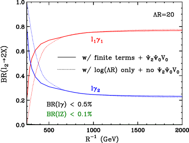
Figure 11: Branching fractions of SU(2)_L-doublet level-2 KK lepton (left) and charged SU(2)_L-singlet level-2 KK lepton (right). Solid curves include finite corrections and new decay channels, while dotted curves are old results.

Figure 12: Branching fraction of SU(2)_L-doublet level-2 KK quark (left) and SU(2)_L-singlet level-2 KK quark (right) for the up-type.

Branching fractions of SU(2)_L doublet quarks are rather complicated as shown in the left panel of Fig. 12. New decay channels $dW$, $ug$ and $uZ$, show branching fractions of $2.5$–$4.5\%$, $1.5$–$2.5\%$ and $1$–$2\%$, respectively.

Branching fractions for neutral KK leptons and the down-type KK quarks are similar. For example, looking at the $d_{2}$ decay we find the $d\gamma_{2}$ and $d_{1}\gamma_{1}$ channels to be dominant with BR $\sim 45\%$, but the branching fraction into $dg$ is slightly higher at about 8%. This is due to the different hypercharge couplings between the up-type and the down-type quarks. Branching fractions into $dZ$ and $d\gamma$ are negligible as before.

Finally we show the branching fractions of level-2 KK top quarks in Fig. 13. In this case we find that the branching fractions of the SU(2)_L doublet KK top into $th$ or $tZ$ are 3–6% each. Other 200 decay modes into $tg$ and $bW^{+}$ show branching fractions of about 2–4% and 1–2%, respectively. The $t\gamma$ branching fraction is below one percent, which implies that the KK top decays directly to two SM particles $\sim$ 8–15% of the time. The SU(2)_L singlet KK top does not have decays to SU(2)_L gauge bosons, and branching fractions for $th$ and $tg$ are of order 1–5.5% and 2–12%, respectively, for $250\,\,\mathrm{GeV}<R^{-1}<2\,\,\mathrm{TeV}$. Due to the Yukawa correction to the KK top mass, two-body decays of level-2 KK top into $W^{+}_{1}B_{1}$, $t_{1}Z_{1}$ and $t\gamma_{2}$ are suppressed for low values of $R^{-1}$.

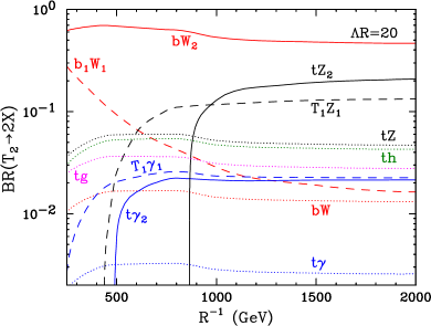
Figure 13: Branching fraction of SU(2)_L-doublet KK top quark (left) and SU(2)_L-singlet KK top quark (right).

5.2.2 $V_{2}$ decays

Fig. 14 shows the branching fractions of $n=2$ KK gauge bosons as a function of $R^{-1}$. Overall, we find our results are similar to those in Ref. [11] with a few notable changes.

Firstly we considered the new decay channels $g_{2}\to gg$, $Z_{2}\to W^{+}W^{-}$, $W^{\pm}_{2}\to ZW^{\pm}$ and $W^{\pm}_{2}\to\gamma W^{\pm}$. Their rather moderate branching fractions contribute with 1–2%, 0.3%, 2–3%, and 0.7%, respectively. The leptonic branching fractions of $Z_{2}$ and $\gamma_{2}$ become smaller with finite corrections and are now about 0.7%.

Due to larger mass corrections for strongly interacting particles (KK-gluon and KK-quarks), only the $n=2$ KK gluon can decay to KK-quarks ($qq_{2}$ or $q_{1}q_{1}$), while two-body decays of KK $Z$ and $W$ gauge bosons into KK quarks are kinematically closed. With finite corrections and additional decay channels, the total decay widths of level-2 bosons increase by a factor of $\sim 2$ for electroweak gauge bosons and $\sim 5$ for KK gluon as shown in Fig. 15. However, their decay widths are still very small due to the phase space suppression of 220 and 211 decays and loop-suppression of 200 decays, as mentioned at the beginning. For electroweak gauge bosons, $\Gamma_{V_{2}}/m_{V_{2}}\lesssim 10^{-3}$, and $\Gamma_{g_{2}}/m_{g_{2}}\sim 0.02$ for KK gluons.

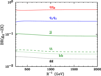
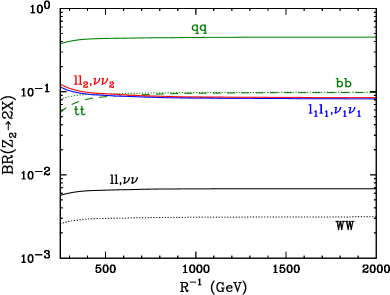
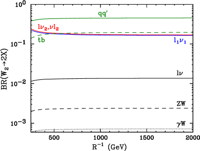
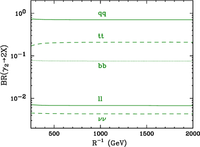
Figure 14: Branching fractions of $\gamma_{2}$, $Z_{2}$, $W_{2}^{\pm}$ and $g_{2}$ for $\Lambda R=20$.

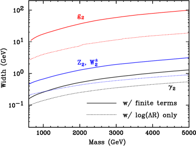
Figure 15: The decay width of level-2 gauge bosons as a function of $R^{-1}$ for $\Lambda R=20$. Solid curves include finite corrections, while dotted curves are old results.

5.3 Cross-sections and signatures

Single production of level-1 KK particles is forbidden due to KK-parity and therefore they must be produced in pairs from collisions of two SM particles or from the decay of level-2 KK particles. However, both single and pair productions are possible for level-2 KK particles. Single production cross sections are suppressed by a loop factor, while pair production cross sections are suppressed by phase space.

All cross sections are calculated at tree level considering five partonic quark flavors in the proton along with the gluon at the 14 TeV LHC. We sum over the final state quark flavors and include charge-conjugated contributions. We used CTEQ6L parton distributions [20] and chose the scale of the strong coupling constant to be equal to the parton-level center-of-mass energy. All results are obtained using CalcHEP [21] based on the implementation of the MUED model from Ref. [16]. Since the particle content and KK number conserving interactions remain the same, we only modified the KK mass spectrum and KK number violating interactions in the existing implementation which is based on Ref. [10]. We also implemented the new interactions which are described throughout our paper.

We summarize single production cross sections of $n=2$ KK gauge bosons (left) and $n=2$ KK quarks (right) in Fig. 16. While overall one observes a slight increase in production cross sections for the KK-gauge bosons, the $gg\to g_{2}$ production channel has been computed for the first time here and contributes at a sizable level. All KK-fermion single production cross sections presented here had also not been considered previously. Fig. 17 shows the pair production of KK quarks (left) and associated production of KK quark and KK gluon (right), respectively.

Another interesting channel is associated production of KK top with SM top quark. $pp\to T_{2}\bar{t}+t\bar{T}_{2}$ is shown as a (black, solid) curve, labeled as ‘$T_{2}t_{0}$’ in the left panel of Fig. 17. Since $T_{2}$ has a large branching fraction into $th$ and a sizable branching fraction into $t\gamma$, $bW$ or $tZ$, this production could be constrained by cross section measurements of SM processes such as $t\bar{t}\gamma$, $t\bar{t}$, $t\bar{t}h$ and $t\bar{t}$.

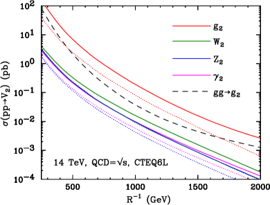
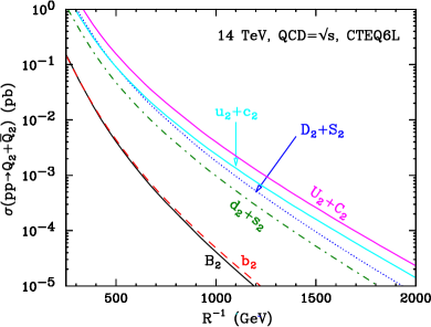
Figure 16: Single production cross section of level-2 KK gauge bosons (left) and level-2 KK fermions (right) as a function of $R^{-1}$. Dotted curves (left) are results from Ref. [11] and solid curves are new results including finite terms. Level-2 fermion cross sections and $\sigma(gg\to g_{2})$ have been computed first time. The cut-off scale has been set to $\Lambda R=20$.

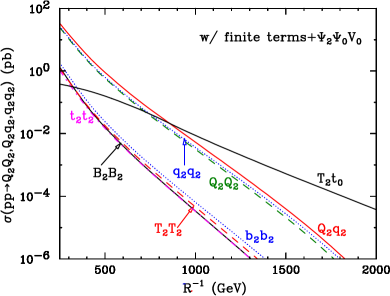
Figure 17: Strong production of $n=2$ KK particles at the 14 TeV LHC. The left panel shows KK-quark pair production, while the right panel shows KK-quark/KK-gluon associated production and KK gluon pair production. Updated results (solid curves) are similar to old results (in dashed curves from Ref. [11]). The cut-off scale has been set to $\Lambda R=20$.

Figure 18: 5$\sigma$ discovery reach for $\gamma_{2}$ (left) and $Z_{2}$ (right). We show the total integrated luminosity ${\cal L}$ (in fb^-1) required for a 5$\sigma$ excess of signal over SM backgrounds in the di-electron (red, dotted) and di-muon (blue, dashed) channels. In each plot, the upper set of curves labeled as ‘DY’ make use of the single production of $\gamma_{2}$ or $Z_{2}$ (from Fig. 16), while the lower set of curves labeled as ‘All processes’ includes indirect $\gamma_{2}$ and $Z_{2}$ productions from $n=2$ KK quarks (see Fig. 17). We assumed the same signal and background efficiencies used in Ref. [11] and combined with our updated cross sections and branching fractions.

Finally, we plot the total integrated luminosity ${\cal L}$ (in fb^-1) required for a 5$\sigma$ excess of signal over background in the di-electron (red, dotted) or di-muon (blue, dashed) channel, as a function of $R^{-1}$ (in GeV). We have used the same backgrounds, basic cuts and detector resolutions as described in Ref. [11]. In each panel of Fig. 18, the upper set of lines labeled ‘DY’ only utilizes the single $V_{2}$ productions from Fig. 16. The lower set of lines (labeled ‘All processes’) includes in addition indirect $\gamma_{2}$ and $Z_{2}$ production from the cascade decays of level-2 KK quarks to level-2 KK gauge bosons from Fig. 17. We do not include contributions from single production of level-2 KK quarks, so as to compare more directly against results in Ref. [11]. They would make a small contribution to the total luminosity as shown in the right panel of Fig. 16.

For both di-electron and di-muon channel, we observe no significant change in the required luminosity compared to results from Ref. [11], although we notice a slight reduction or increase in the luminosity, depending on the value of $R^{-1}$. This is due to the interplay between improved results on cross sections and branching fractions. Overall, production cross sections are increased as shown in Figs. 16 and 17, while branching fractions decrease as shown Fig. 14. The high-luminosity LHC with 3 ab^-1 would be able to probe the level-2 KK photon up to $R^{-1}\sim 1.2$ TeV in the $\mu^{+}\mu^{-}$ and $R^{-1}\sim 1.5$ TeV in the $e^{+}e^{-}$ channel. The corresponding reach for the level-2 KK $Z$ boson is lower due to the relevant branching fractions.

6 Conclusions

In this article we presented the one-loop corrected mass spectrum and KK-number violating decays of level-2 KK states into SM particles in models with universal extra dimensions. As a concrete framework we chose to add one additional universal extra dimension to the SM, which is compactified on a circle with a $\mathbb{Z}_{2}$ orbifold. Due to its non-renormalizability the model is regarded as an effective low-energy theory with a hard cutoff scale $\Lambda$ at which an unspecified UV-completion is expected to describe the physics. This enables us to write down sensible $\overline{\text{MS}}$ counterterms with a logarithmic sensitivity to the cutoff. All calculations were performed in the 4D effective theory using publicly available software supplemented by in-house routines.

The self energy diagrams giving rise to the mass corrections contain an infinite tower of states in the loop, whose summation requires additional regularization. To this end we employed the Poisson summation identity to identify the divergent pieces in winding number space and remove them. The results can be divided into logarithmically divergent boundary terms and finite bulk contributions.

The low cutoff scale ($\Lambda R\lesssim 50$, considering perturbativity and unitarity [1, 13]) implies that the leading (logarithmic) terms in the one-loop corrections to KK masses are not as large as those in supersymmetry, and finite contributions could play an important role phenomenologically.

When including the new finite (non-logarithmic) corrections, the mass spectrum broadens and each KK particle becomes heavier, which implies that the pair production cross sections of level-1 KK particles at colliders would be reduced but their acceptance rate would increase. We also examined the nature of the NLKP, and confirmed that it is always the right-handed KK lepton, which is different from what has been stated in the literature, where the NLKP was thought to be the KK-Higgs for a large KK scale. The KK Weinberg angles are further reduced such that weak eigenstates are basically mass eigenstates.

Using the same methodology, we have calculated finite corrections to the decays of level-2 KK states into SM particles, including previously unknown couplings. Since the interactions violate KK number, only a finite number of diagrams contribute to the vertices and no additional regularization is necessary. We then revisited the computation of branching fractions for level-2 KK particles. For KK fermions the basic features remain the same as before with the addition of new decay modes opening up at the few-percent level. The largest effects appear in the decay of level-2 KK top quarks, i.e., the branching fraction of the left-handed KK top quark into $th$ is about 20–30%. Branching fractions of level-2 gauge bosons are also updated. Overall, the decay widths of level-2 particles are observed to increase when these effects are included, but they are still narrower than the detector resolution.

Finally, we would like to make a few comments about other potentially interesting collider and dark matter phenomenology. In this paper, we showed results for the production of level-2 KK gauge bosons at the LHC. It is desirable to study these with a more detailed simulation, including single and pair production of level-2 KK fermions, and set bounds on ($R^{-1}$, $\Lambda R$) from various resonance searches, such as $V_{2}$ decays to $\ell\bar{\ell}$, $jj$, $W^{+}W^{-}$, $W^{\pm}Z$, $ZZ$, $t\bar{t}$. Here one can make use of boosted $W$, $Z$ and $t$ event topologies.

The collider phenomenology of singly produced level-2 KK fermions provides interesting signatures. For instance, searches for excited quarks in various final states would constrain level-2 decays such as $pp\to Q_{2}/q_{2}\to q^{\prime}V$, where $V$ = $\gamma$, $Z$, $W$ or $g$. $Q_{2}$ or $q_{2}$ could appear as a single three-jet resonance via $q^{\prime}V_{2}$ with $V_{2}\to f_{0}f_{0}^{\prime}$. Other interesting topologies involve the top quark and the Higgs. They may not provide the best sensitivity in a search for this particular model since certain signal-to-background ratios may be small. However they could serve as a benchmark model for various searches and provide useful search grounds. We list a few examples below.

• $pp\to t_{2}\bar{t}_{2}$ with $t_{2}\to th$, $t_{2}\to tg$ or $t_{2}\to t\gamma$

• $pp\to T_{2}\bar{T}_{2}$ with $T_{2}\to th$, $T_{2}\to Zt$, $T\to tg$, $T\to t\gamma$ or $T_{2}\to t\gamma_{2}$ $(\gamma_{2}\to t\bar{t})$

• $pp\to B_{2}\bar{B}_{2}$ with $B_{2}\to Zb$ or $B_{2}\to Wt$ (and small branching fractions to $B_{2}\to gb$, $B_{2}\to b\gamma$)

• $pp\to b_{2}\bar{b}_{2}$ with $b_{2}\to gb$ (and small branching fractions to $b_{2}\to\gamma b$, and $b_{2}\to Zb$)

• $pp\to Q_{2},\,q_{2},\,Q_{2}\bar{Q}_{2},\,q_{2}\bar{q}_{2}$ (both single and pair production) with $Q_{2}\to qg$ or $Q_{2}\to q\gamma$

• $T_{2}\bar{T}_{2}\to t\bar{t}h+X$ (inclusive $t\bar{t}h$ production)

As discussed earlier, level-1 KK particles are always produced in pairs due to KK parity and lead to signals with missing transverse momentum. Final states with jets + leptons + missing transverse momentum are known to provide stringent bounds on $R^{-1}$ (see Ref. [9]). It is worth revisiting these analyses with our improved mass spectrum, since the broader mass pattern will lead to signal efficiency gains while at the same time the increased masses will reduce the production cross sections.

The computation of the relic abundance of KK dark matter has a rather long history [2, 3, 4]. Ref. [4] includes both coannihilation and resonance effects, which play a crucial role in increasing the preferred mass scale of the KK photon. Our results imply that a slightly broader mass spectrum would reduce effective cross sections in the coannihilation processes (which are suppressed by $\frac{e^{-x_{f}^{\prime}(m^{\prime}_{1}-m^{\prime}_{\gamma_{1}})}}{e^{-x_{f}(m_{1}-m_{\gamma_{1}})}}\approx e^{-x_{f}(m^{\prime}_{1}-m_{1})}$ where $x_{f}\approx x_{f}^{\prime}$ is the freeze-out temperature and $m_{1}$ is the mass of the coannihilating particle, $m_{1}^{\prime}$ is the improved mass, and $m_{\gamma_{1}}\approx m_{\gamma_{1}}^{\prime}$ is the mass of KK photon), pushing $m_{\gamma_{1}}$ to a lower value. However, $11\to 20$ processes with the level-2 particle decaying to two zero modes would increase the effective annihilation cross section efficiently, increasing the preferred value for $m_{\gamma_{1}}$. This is a highly non-trivial and complicated exercise and we postpone it to a follow-up study.

We hope that our results will be useful for investigations of the phenomenology of universal extra dimensions and also provide interesting event topologies for various collider searches [22].

Appendix A Feynman rules of MUED

This appendix lists a complete set of Standard Model Lagrangian in a universal extra dimensions model in 5 dimensions with a $S^{1}/\mathbb{Z}_{2}$ orbifold compactification. The conventions are chosen such that Greek indices take values $0,1,2,3$, assigned to the uncompactified dimensions, while capital Latin indices describe the full 5D theory, where the extra spatial dimension is denoted as $x^{5}$ where necessary. The 5D coupling constants are labeled with a superscript $(5)$ and are related to the 4D effective couplings through

$$g =\frac{g^{(5)}}{\sqrt{\pi R}}\,, h_{i} =\frac{h_{i}^{(5)}}{\sqrt{\pi R}}\,, \lambda =\frac{\lambda^{(5)}}{\pi R}\,,$$ (58)

for the gauge, Yukawa and Higgs self coupling respectively.

Furthermore we have to define the conventions for the extension of the Clifford algebra,

$$\Gamma^{M} =\left(\gamma^{\mu},i\gamma^{5}\right)\,,\quad\text{such that}\quad\left\{\Gamma^{M},\Gamma^{N}\right\}=2g^{MN},$$ (59)

where $g^{MN}$ is the 5D metric tensor

$$g_{MN} =\begin{pmatrix}g_{\mu\nu}&0\\ 0&-1\end{pmatrix},$$ (60)

and $g^{\mu\nu}=\text{diag}\{+---\}$ the usual 4D metric. It is also helpful to define an extended set of $\Delta$ symbols [16]

$$\Delta_{mnl}^{1}=\delta_{l,m+n}+\delta_{n,l+m}+\delta_{m,l+n}\,,$$

$$\Delta_{mnlk}^{2}=\delta_{k,l+m+n}+\delta_{l,m+n+k}+\delta_{m,n+k+l}+\delta_{n,k+l+m}+\delta_{k+m,l+n}+\delta_{k+l,m+n}+\delta_{k+n,l+m}\,,$$

$$\Delta_{mnlk}^{3}=-\delta_{k,l+m+n}-\delta_{l,m+n+k}-\delta_{m,n+k+l}-\delta_{n,k+l+m}+\delta_{k+l,m+n}+\delta_{k+m,l+n}+\delta_{k+n,l+m}\,,$$

$$\Delta_{mnl}^{4}=-\delta_{l,m+n}+\delta_{n,l+m}+\delta_{m,l+n}\,,$$

$$\Delta_{mnlk}^{5}=-\delta_{k,l+m+n}-\delta_{l,m+n+k}+\delta_{m,n+k+l}+\delta_{n,k+l+m}-\delta_{k+l,m+n}+\delta_{k+m,l+n}+\delta_{k+n,l+m}\,.$$ (61)

A.1 The Gauge Sector

As a generic example, we show the gauge sector Lagrangian for a single vector field in the adjoint representation of SU($N$), which contains a four-component vector $V_{\mu}\left(x,x^{5}\right)$ and a fifth component $V_{5}\left(x,x^{5}\right)$, which takes the role of a Goldstone boson. Additionally we require the ghost field $c\left(x,x^{5}\right)$. After compactification the Lagrangians read

$$\mathcal{L}_{\rm Gauge}= \frac{1}{2}\int_{-\pi R}^{\pi R}dx^{5}\,\left\{-\frac{1}{4}F^{a}_{MN}F^{a,MN}\right\}=\frac{1}{2}\int_{-\pi R}^{\pi R}dx^{5}\,\left\{-\frac{1}{4}F^{a}_{\mu\nu}F^{a,\mu\nu}-\frac{1}{2}F^{a}_{5\nu}F^{a,5\nu}\right\}\,,$$

$$\mathcal{L}_{\rm GF}= \frac{1}{2}\int_{-\pi R}^{\pi R}dx^{5}\,\left\{-\frac{1}{2\xi}\left(\partial^{\mu}V^{a}_{\mu}\left(x,x^{5}\right)-\xi\partial_{5}V_{5}^{a}\left(x,x^{5}\right)\right)^{2}\right\}\,,$$

$$\mathcal{L}_{\rm Ghost}= \frac{1}{2}\int_{-\pi R}^{\pi R}dx^{5}\,\left\{\overline{c}^{a}\left(x,x^{5}\right)\left(-\partial^{\mu}\partial_{\mu}+\xi\partial_{5}^{2}\right)c^{a}\left(x,x^{5}\right)\right.$$

$$\left.+g^{(5)}f^{abc}\left(-\partial^{\mu}\overline{c}^{a}\left(x,x^{5}\right)V_{\mu}^{c}\left(x,x^{5}\right)c^{b}\left(x,x^{5}\right)+\xi\partial_{5}\overline{c}^{a}\left(x,x^{5}\right)V_{5}^{c}c^{b}\left(x,x^{5}\right)\right)\right\}\;,$$ (62)

with $\xi$ being the gauge parameter in the generalized $R_{\xi}$ gauge. After decomposing the 5D fields into Fourier modes, according to

$$V_{\mu}\left(x,x^{5}\right) =\frac{1}{\sqrt{\pi R}}\biggl{[}V_{\mu}^{0}(x)+\sqrt{2}\sum_{n=1}^{\infty}V_{\mu}^{n}(x)\,\cos\frac{nx^{5}}{R}\biggr{]}\,,$$

$$V_{5}\left(x,x^{5}\right) =\sqrt{\frac{2}{\pi R}}\sum_{n=1}^{\infty}V_{5}^{n}(x)\,\sin\frac{nx^{5}}{R}\,,$$

$$c^{a}\left(x,x^{5}\right) =\frac{1}{\sqrt{\pi R}}\biggl{[}c^{0,a}(x)+\sqrt{2}\sum_{n=1}^{\infty}c^{n,a}(x)\,\cos\frac{nx^{5}}{R}\biggr{]}\,,$$ (63)

and performing the integral over the fifth dimension one obtains the effectively 4D pure Yang-Mills pieces, given by

$$\frac{1}{2}\int_{-\pi R}^{\pi R}dx^{5}\,\left(F^{a}_{5\nu}F^{a5\nu}\right) =-\sum_{n=1}^{\infty}\left(\frac{n}{R}V^{n,a}_{\mu}+\partial_{\mu}V^{n}_{5}-gC^{abc}V^{n,b}_{5}V^{0,c}_{\mu}\right)^{2}$$

$$+\sum_{m,n,l=1}^{\infty}\sqrt{2}gC^{ade}\left(\frac{m}{R}V^{m,a}_{\mu}+\partial_{\mu}V^{m,a}_{5}-gC^{abc}V^{m,b}_{5}V^{0,c}_{\mu}\right)V^{n,d}_{5}V^{l,e\mu}\Delta^{4}_{mnl}$$

$$-\frac{g^{2}}{2}C^{abc}C^{ade}\sum_{m,n,l,k=1}^{\infty}V^{m,b}_{5}V^{n,c}_{\mu}V^{l,d}_{5}V^{k,e\mu}\Delta^{5}_{mlnk}\,,$$ (64)

$$\frac{1}{2}\int_{-\pi R}^{\pi R}dx^{5}\,\left(F^{a}_{\mu\nu}F^{a\mu\nu}\right) =F^{0,a}_{\mu\nu}F^{0,a\mu\nu}+2gC^{abc}\sum_{n=1}^{\infty}F^{0,a}_{\mu\nu}V^{n,b\mu}V^{n,c\nu}+\sum_{n=1}^{\infty}\left(\partial_{\mu}V^{n,a}_{\nu}-\partial_{\nu}V^{n,a}_{\mu}\right)^{2}$$

$$+2gC^{abc}\sum_{n=1}^{\infty}\left(\partial_{\mu}V^{n,a}_{\nu}-\partial_{\nu}V^{n,a}_{\mu}\right)\left(V^{0,b\mu}V^{n,c\nu}+V^{0,c\nu}V^{n,b\mu}\right)$$

$$+\sqrt{2}gC^{abc}\sum_{m,n,l=1}^{\infty}\left(\partial_{\mu}V^{m,a}_{\nu}-\partial_{\nu}V^{m,a}_{\mu}\right)V^{n,b\mu}V^{l,c\nu}\Delta^{1}_{mnl}$$

$$+\sum_{n=1}^{\infty}g^{2}(C^{abc}(V^{0,b}_{\mu}V^{n,c}_{\nu}+V^{0,c}_{\nu}V^{n,b}_{\mu}))^{2}$$

$$+\sqrt{2}g^{2}\sum_{m,n,l=1}^{\infty}C^{abc}C^{ade}\left(V^{0,b}_{\mu}V^{m,c}_{\nu}+V^{0,c}_{\nu}V^{m,b}_{\mu}\right)V^{n,d\mu}V^{l,e\nu}\Delta^{1}_{mnl}$$

$$+\sum_{m,n,l,k=1}^{\infty}\frac{g^{2}}{2}C^{abc}C^{ade}V^{m,b}_{\mu}V^{n,c}_{\nu}V^{l,d\mu}V^{k,e\nu}\Delta^{2}_{mnlk},$$ (65)

a gauge fixing part given by

$$\mathcal{L}_{\rm GF}=-\frac{1}{2\xi}\biggl{[}\left(\partial^{\mu}V_{\mu}^{0}\right)^{2}+\sum_{n=1}^{\infty}\Bigl{(}\partial^{\mu}V_{\mu}^{n}-\frac{\xi n}{R}V_{5}^{n}\Bigr{)}^{2}\biggr{]},$$ (66)

and finally the ghost piece

$$\mathcal{L}_{\rm Ghost}= -\overline{c}^{0,a}\partial^{\mu}\partial_{\mu}c^{0,a}-gf^{abc}\partial^{\mu}\overline{c}^{0,a}V_{\mu}^{0,c}c^{0,b}-\sum_{n=1}^{\infty}\left[\overline{c}^{n,a}\partial^{\mu}\partial_{\mu}c^{n,a}+\xi\frac{n^{2}}{R^{2}}\overline{c}^{n,a}c^{n,a}\right]$$

$$-gf^{abc}\sum_{n=1}^{\infty}\left[\partial^{\mu}\overline{c}^{0,a}V^{n,c}_{\mu}c^{n,b}+\partial^{\mu}\overline{c}^{n,a}V^{0,c}_{\mu}c^{n,b}+\partial^{\mu}\overline{c}^{n,a}V_{\mu}^{n,c}c^{0,b}+\xi\frac{n}{R}\overline{c}^{n,a}V_{5}^{n,b}c^{0,c}\right]$$

$$-\frac{g}{\sqrt{2}}f^{abc}\sum_{m,n,l=1}^{\infty}\left[\partial^{\mu}\overline{c}^{l,a}V^{m,c}_{\mu}c^{n,b}\Delta^{1}_{lmn}+\xi\frac{l}{R}\overline{c}^{l,a}V^{m,c}_{5}c^{n,b}\Delta^{4}_{lmn}\right].$$ (67)

A.2 The Fermion Sector

Analogously, we show the Lagrangian for a fermion in the fundamental representation coupled to a generic SU($N$) gauge field. The structure of the SM makes it necessary to distinguish between Fermions $\Psi$ that transform as doublets under SU(2) and those that are singlets $\psi$. Their respective decomposition is

$$\Psi\left(x,x^{5}\right) =\frac{1}{\sqrt{\pi R}}\left\{\Psi_{L}(x)+\sqrt{2}\sum_{n=1}^{\infty}\left[P_{-}\Psi_{L}^{n}(x)\,\cos\frac{nx^{5}}{R}+P_{+}\Psi_{R}^{n}(x)\,\sin\frac{nx^{5}}{R}\right]\right\},$$

$$\psi\left(x,x^{5}\right) =\frac{1}{\sqrt{\pi R}}\left\{\psi_{R}(x)+\sqrt{2}\sum_{n=1}^{\infty}\left[P_{+}\psi_{R}^{n}(x)\,\cos\frac{nx^{5}}{R}+P_{-}\psi_{L}^{n}(x)\,\sin\frac{nx^{5}}{R}\right]\right\}.$$ (68)

The generic Lagrangian for either of the Fermions coupling to $V_{M}\left(x,x^{5}\right)$ can be written as

$${\cal L}_{\Psi} =\frac{1}{2}\int_{-\pi R}^{\pi R}dx^{5}\,\left\{i\bar{\Psi}\left(x,x^{5}\right)\Gamma^{M}\left[\partial_{M}+i{g^{(5)}}V_{M}\left(x,x^{5}\right)\right]\Psi\left(x,x^{5}\right)\right\}$$

$$=i\bar{\Psi}_{L}\gamma^{\mu}\left(\partial_{\mu}+i{g}V^{0}_{\mu}\right)\Psi_{L}-\sum_{n=1}^{\infty}\frac{n}{R}\left[\bar{\Psi}^{n}_{R}\Psi^{n}_{L}+\bar{\Psi}^{n}_{L}\Psi^{n}_{R}\right]$$

$$+\sum_{n=1}^{\infty}\left[i\bar{\Psi}^{n}_{R}\gamma^{\mu}\left(\partial_{\mu}+i{g}V^{0}_{\mu}\right)\Psi^{n}_{R}+i\bar{\Psi}^{n}_{L}\gamma^{\mu}\left(\partial_{\mu}+i{g}V^{0}_{\mu}\right)\Psi^{n}_{L}-g\bar{\Psi}_{L}\gamma^{\mu}V^{n}_{\mu}\Psi^{n}_{L}+g\bar{q}_{L}i\gamma^{5}V^{n}_{5}\Psi^{n}_{R}\right]$$

$$-\frac{g}{\sqrt{2}}\sum_{m,n,l=1}^{\infty}\left[\bar{\Psi}^{m}_{L}\gamma^{\mu}V^{n}_{\mu}\Psi^{l}_{L}\Delta^{1}_{mnl}+\bar{\Psi}^{m}_{R}\gamma^{\mu}V^{n}_{\mu}\Psi^{l}_{R}\Delta^{4}_{mln}+\bar{\Psi}^{m}_{L}i\gamma^{5}V^{n}_{5}\Psi^{l}_{R}\Delta^{4}_{lnm}\right].$$ (69)

A.3 The Higgs Sector

Due to the somewhat complicated structure of the four-point interactions between the Higgs and electroweak gauge bosons, we here show the Higgs Lagrangian not just for a generic gauge group, but write the explicit Lagrangian for a Higgs doublet coupling to the U(1)_Y field $B_{M}\left(x,x^{5}\right)$ and the SU(2)_L field $W_{M}\left(x,x^{5}\right)$.

The Higgs doublet $\Phi\left(x,x^{5}\right)$ is decomposed as

$$\Phi\left(x,x^{5}\right) =\frac{1}{\sqrt{\pi R}}\left\{\Phi_{0}(x)+\sqrt{2}\sum_{n=1}^{\infty}\Phi_{n}(x)\,\cos\frac{nx^{5}}{R}\right\}$$ (70)

and inserted into the Lagrangian

$${\cal L}_{\rm Higgs} =\frac{1}{2}\int_{-\pi R}^{\pi R}dx^{5}\,\left[\left(D_{M}\Phi\left(x,x^{5}\right)\right)^{\dagger}\left(D^{M}\Phi\left(x,x^{5}\right)\right)+\mu^{2}\Phi^{\dagger}\left(x,x^{5}\right)\Phi\left(x,x^{5}\right)-\lambda\left(\Phi^{\dagger}\left(x,x^{5}\right)\Phi\left(x,x^{5}\right)\right)^{2}\right]$$

$$=\left[\left(\partial_{\mu}+i{g_{2}}W^{0}_{\mu}+\frac{i{g_{1}}}{2}B^{0}_{\mu}\right)\Phi_{0}\right]^{\dagger}\left[\left(\partial^{\mu}+i{g_{2}}W^{0\mu}+\frac{i{g_{1}}}{2}B^{0\mu}\right)\Phi_{0}\right]$$

$$+\sum_{n=1}^{\infty}\left[\left(\partial_{\mu}+i{g_{2}}W^{0}_{\mu}+\frac{i{g_{1}}}{2}B^{0}_{\mu}\right)\Phi_{n}\right]^{\dagger}\left[\left(\partial^{\mu}+i{g_{2}}W^{0\mu}+\frac{i{g_{1}}}{2}B^{0\mu}\right)\Phi_{n}\right]$$

$$+i{g_{2}}\sum_{n=1}^{\infty}\left[(\partial^{\mu}\Phi_{0})^{\dagger}W^{n}_{\mu}\Phi_{n}+(\partial^{\mu}\Phi_{n})^{\dagger}W^{n}_{\mu}\Phi_{0}-\Phi_{n}^{\dagger}{W^{n}_{\mu}}^{\dagger}(\partial^{\mu}\Phi_{0})-\Phi_{0}^{\dagger}{W^{n}_{\mu}}^{\dagger}(\partial^{\mu}\Phi_{n})\right]$$

$$+i{g_{2}}\sum_{m,n,l=1}^{\infty}\left[(\partial^{\mu}\Phi_{m})^{\dagger}W^{n}_{\mu}\Phi_{l}-\Phi_{l}^{\dagger}{W^{n}_{\mu}}^{\dagger}(\partial^{\mu}\Phi_{m})\right]\Delta^{1}_{mnl}$$

$$+\frac{i{g_{1}}}{2}\sum_{n=1}^{\infty}\left[(\partial^{\mu}\Phi_{0})^{\dagger}B^{n}_{\mu}\Phi_{n}+(\partial^{\mu}\Phi_{n})^{\dagger}B^{n}_{\mu}\Phi_{0}-\Phi_{n}^{\dagger}B^{n}_{\mu}(\partial^{\mu}\Phi_{0})-\Phi_{0}^{\dagger}B^{n}_{\mu}(\partial^{\mu}\Phi_{n})\right]$$

$$+\frac{i{g_{1}}}{2\sqrt{2}}\sum_{m,n,l=1}^{\infty}\left[(\partial^{\mu}\Phi_{m})^{\dagger}B^{n}_{\mu}\Phi_{l}-\Phi_{l}^{\dagger}B^{n}_{\mu}(\partial^{\mu}\Phi_{m})\right]\Delta^{1}_{mnl}$$

$$+g_{2}^{2}\sum_{n=1}^{\infty}\left[\Phi_{0}^{\dagger}{W^{0}_{\mu}}^{\dagger}W^{n\mu}\Phi_{n}+\Phi_{n}^{\dagger}{W^{0}_{\mu}}^{\dagger}W^{n\mu}\Phi_{0}+\Phi_{0}^{\dagger}{W^{n\mu}}^{\dagger}W^{0}_{\mu}\Phi_{n}+\Phi_{0}^{\dagger}{W^{n\mu}}^{\dagger}W^{n}_{\mu}\Phi_{0}+\Phi_{n}^{\dagger}{W^{n\mu}}^{\dagger}W^{0}_{\mu}\Phi_{0}\right]$$

$$+\frac{g_{2}^{2}}{\sqrt{2}}\sum_{m,n,l=1}^{\infty}\left[\Phi_{m}^{\dagger}{W^{0}_{\mu}}^{\dagger}W^{n\mu}\Phi_{l}+\Phi_{0}^{\dagger}{W^{m}_{\mu}}^{\dagger}W^{l\mu}\Phi_{n}+\Phi_{m}^{\dagger}{W^{n}_{\mu}}^{\dagger}W^{0\mu}\Phi_{l}+\Phi_{m}^{\dagger}{W^{n}_{\mu}}^{\dagger}W^{l\mu}\Phi_{0}\right]\Delta^{1}_{mnl}$$

$$+\frac{g_{2}^{2}}{2}\sum_{m,n,l,k=1}^{\infty}\left[\Phi_{m}^{\dagger}{W^{n}_{\mu}}^{\dagger}W^{l\mu}\Phi_{k}\right]\Delta^{2}_{mnlk}$$

$$+\frac{{g_{1}}{g_{2}}}{2}\sum_{n=1}^{\infty}\left[\Phi_{0}^{\dagger}{W^{0}_{\mu}}^{\dagger}B^{n\mu}\Phi_{n}+\Phi_{n}^{\dagger}{W^{0}_{\mu}}^{\dagger}B^{n\mu}\Phi_{0}+\Phi_{0}^{\dagger}{W^{n}_{\mu}}^{\dagger}B^{0\mu}\Phi_{n}+\Phi_{0}^{\dagger}{W^{n}_{\mu}}^{\dagger}B^{n\mu}\Phi_{0}+\Phi_{n}^{\dagger}{W^{n}_{\mu}}^{\dagger}B^{0\mu}\Phi_{0}\right.$$

$$\hskip 71.13188pt+\Phi_{n}^{\dagger}B^{n\mu}W^{0}_{\mu}\Phi_{0}+\Phi_{0}^{\dagger}B^{n\mu}W^{0}_{\mu}\Phi_{n}+\Phi_{n}^{\dagger}B^{0\mu}W^{n}_{\mu}\Phi_{0}+\Phi_{0}^{\dagger}B^{n\mu}W^{n}_{\mu}\Phi_{0}+\Phi_{0}^{\dagger}B^{0\mu}W^{n}_{\mu}\Phi_{n}\left.\right]$$

$$+\frac{{g_{1}}{g_{2}}}{2\sqrt{2}}\sum_{m,n,l=1}^{\infty}\left[\Phi_{m}^{\dagger}{W^{0}_{\mu}}^{\dagger}B^{n\mu}\Phi_{l}+\Phi_{0}^{\dagger}{W^{m}_{\mu}}^{\dagger}B^{l\mu}\Phi_{n}+\Phi_{m}^{\dagger}{W^{n}_{\mu}}^{\dagger}B^{0\mu}\Phi_{l}+\Phi_{m}^{\dagger}{W^{n}_{\mu}}^{\dagger}B^{l\mu}\Phi_{0}\right.$$

$$\hskip 71.13188pt+\Phi_{l}^{\dagger}B^{n\mu}W^{0}_{\mu}\Phi_{m}+\Phi_{n}^{\dagger}B^{l\mu}W^{m}_{\mu}\Phi_{0}+\Phi_{l}^{\dagger}B^{0\mu}W^{n}_{\mu}\Phi_{m}+\Phi_{0}^{\dagger}B^{l\mu}W^{n}_{\mu}\Phi_{m}\left.\right]\Delta^{1}_{mnl}$$

$$+\frac{{g_{1}}{g_{2}}}{4}\sum_{m,n,l,k=1}^{\infty}\left[\Phi_{m}^{\dagger}{W^{n}_{\mu}}^{\dagger}B^{l\mu}\Phi_{k}+\Phi_{k}^{\dagger}B^{l\mu}W^{n}_{\mu}\Phi_{m}\right]\Delta^{2}_{mnlk}$$

$$+\frac{g_{1}^{2}}{4}\sum_{n=1}^{\infty}\left[2\Phi_{0}^{\dagger}B^{0}_{\mu}B^{n\mu}\Phi_{n}+2\Phi_{n}^{\dagger}B^{0}_{\mu}B^{n\mu}\Phi_{0}+\Phi_{0}^{\dagger}B^{n}_{\mu}B^{n\mu}\Phi_{0}\right]$$

$$+\frac{g_{1}^{2}}{4\sqrt{2}}\sum_{m,n,l=1}^{\infty}\left[2\Phi_{m}^{\dagger}B^{0}_{\mu}B^{n\mu}\Phi_{l}+\Phi_{0}^{\dagger}B^{m}_{\mu}B^{l\mu}\Phi_{n}+\Phi_{m}^{\dagger}B^{n}_{\mu}B^{l\mu}\Phi_{0}\right]\Delta^{1}_{mnl}$$

$$+\frac{g_{1}^{2}}{4}\sum_{m,n,l,k=1}^{\infty}\left[\Phi_{m}^{\dagger}B^{n}_{\mu}B^{l\mu}\Phi_{k}\right]\Delta^{2}_{mnlk}$$

$$+\mu^{2}\left[\Phi_{0}^{\dagger}\Phi_{0}+\sum_{n=1}^{\infty}\Phi_{n}^{\dagger}\Phi_{n}\right]-\sum_{n=1}^{\infty}\left(\frac{n}{R}\right)^{2}\Phi_{n}^{\dagger}\Phi_{n}$$

$$+\frac{1}{\sqrt{2}}\sum_{m,n,l=1}^{\infty}\frac{n}{R}\Phi_{n}^{\dagger}\left(\frac{i{g_{1}}}{2}B^{m}_{5}+i{g_{2}}{W^{m}_{5}}\right)\Phi_{l}\Delta^{4}_{mnl}$$

$$-\frac{1}{\sqrt{2}}\sum_{m,n,l=1}^{\infty}\frac{m}{R}\Phi_{l}^{\dagger}\left(\frac{i{g_{1}}}{2}B^{n}_{5}+i{g_{2}}W^{n}_{5}\right)\Phi_{m}\Delta^{4}_{mnl}$$

$$-\frac{1}{2}\sum_{m,n,l,k=1}^{\infty}\Phi_{l}^{\dagger}\left(\frac{i{g_{1}}}{2}B^{m}_{5}+i{g_{2}}{W^{m}_{5}}^{\dagger}\right)\left(\frac{i{g_{1}}}{2}B^{n}_{5}+i{g_{2}}W^{n}_{5}\right)\Phi_{k}\Delta^{5}_{mnlk}$$

$$-\sum_{n=1}^{\infty}\left[\Phi_{0}^{\dagger}\left(g_{2}W_{5}^{n}+\frac{g_{1}}{2}B_{5}^{n}\right)^{2}\Phi_{0}+\frac{n}{R}\Phi_{0}^{\dagger}\left(g_{2}W_{5}^{n}+\frac{g_{1}}{2}B_{5}^{n}\right)\Phi_{n}-\frac{n}{R}\Phi_{n}^{\dagger}\left(g_{2}W_{5}^{n}+\frac{g_{1}}{2}B_{5}^{n}\right)\Phi_{0}\right]$$

$$-\frac{1}{\sqrt{2}}\sum_{m,n,l=1}^{\infty}\left[\Phi_{0}^{\dagger}\left(g_{2}W_{5}^{k}+\frac{g_{1}}{2}B_{5}^{k}\right)\left(g_{2}W_{5}^{l}+\frac{g_{1}}{2}B_{5}^{l}\right)\Phi_{m}\right.$$

$$\hskip 71.13188pt\left.+\Phi_{m}^{\dagger}\left(g_{2}W_{5}^{k}+\frac{g_{1}}{2}B_{5}^{k}\right)\left(g_{2}W_{5}^{l}+\frac{g_{1}}{2}B_{5}^{l}\right)\Phi_{0}\right]\Delta^{4}_{klm}$$

$$-\lambda\left(\Phi_{0}^{\dagger}\Phi_{0}\right)^{2}-\lambda\sum_{n=1}^{\infty}\left[\left(\Phi_{0}^{\dagger}\Phi_{n}+\Phi_{n}^{\dagger}\Phi_{0}\right)^{2}+2\Phi_{0}^{\dagger}\Phi_{0}\Phi_{n}^{\dagger}\Phi_{n}\right]$$

$$-\sqrt{2}\lambda\sum_{m,n,l=1}^{\infty}\Phi_{m}^{\dagger}\Phi_{n}\left(\Phi_{l}^{\dagger}\Phi_{0}+\Phi_{0}^{\dagger}\Phi_{l}\right)\Delta^{1}_{mnl}-\frac{\lambda}{2}\sum_{m,n,l,k=1}^{\infty}\Phi_{m}^{\dagger}\Phi_{n}\Phi_{l}^{\dagger}\Phi_{k}\Delta^{2}_{mnlk}\,.$$ (71)

A.4 The Yukawa Sector

To ensure that the SM Fermions acquire a mass through EWSB one has to consider the Yukawa couplings to the Higgs field. For a down-type fermion they are described by

$$\mathcal{L}_{\rm Yukawa} =\frac{1}{2}\int_{-\pi R}^{\pi R}dx^{5}\,\left\{h^{(5)}_{i}\bar{\Psi}\left(x,x^{5}\right)\psi\left(x,x^{5}\right)\Phi\left(x,x^{5}\right)\right\}$$

$$=h_{i}\bar{\Psi}_{L}\psi_{R}\Phi_{0}+h_{i}\sum_{n=1}^{\infty}\left[\bar{\Psi}^{n}_{L}\psi^{n}_{R}\Phi_{0}+\bar{\Psi}^{n}_{R}\psi^{n}_{L}\Phi_{0}\right]+h_{i}\sum_{n=1}^{\infty}\left[\bar{\Psi}_{L}\psi^{n}_{R}\Phi_{n}+\bar{\Psi}^{n}_{L}\psi_{R}\Phi_{n}\right]$$

$$+\frac{h_{i}}{\sqrt{2}}\sum_{m,n,l=1}^{\infty}\left[\bar{\Psi}^{n}_{L}\psi^{m}_{R}\Phi_{l}\Delta^{1}_{mnl}+\bar{\Psi}^{n}_{R}\psi^{m}_{L}\Phi_{l}\Delta^{4}_{mnl}\right].$$ (72)

and for an up-type fermion they can be constructed in complete analogy.

Appendix B KK-number violating couplings in MUED

In this appendix, the KK-number violating couplings discussed in section 4 are shown for the MUED extension of the SM. Here $g_{1,2,3}$ are the couplings of the SM U(1)_Y, SU(2)_L and SU(3)_C gauge groups, respectively, while $h_{t}$ is the top Yukawa coupling and $\lambda_{H}$ the Higgs self-coupling. The $L_{n}$ is defined as $L_{n}\equiv\ln(\Lambda^{2}/m_{n}^{2})$.

$\bar{\psi}_{0}$–$\psi_{0}$–$V_{2}^{\mu}$ coupling:

$-iC_{\psi_{0}\psi_{0}V_{2}}\gamma^{\mu}T^{a}P_{\pm}\,$

$$C_{Q_{0}Q_{0}G_{2}} =\frac{\sqrt{2}g_{3}}{64\pi^{2}}\biggl{[}\begin{aligned} &g_{3}^{2}\biggl{(}11L_{1}+35-\frac{11\pi^{2}}{3}\biggr{)}+g_{2}^{2}\biggl{(}-\frac{27}{4}L_{1}-\frac{39}{4}+\frac{21\pi^{2}}{16}\biggr{)}\\ &+g_{1}^{2}\biggl{(}-\frac{1}{4}L_{1}-\frac{13}{36}+\frac{7\pi^{2}}{144}\biggr{)}\biggr{]}\end{aligned}$$ (73)

$$C_{t_{L0}t_{L0}G_{2}} =C_{b_{L0}b_{L0}G_{2}}$$

$$=\frac{\sqrt{2}g_{3}}{64\pi^{2}}\biggl{[}\begin{aligned} &g_{3}^{2}\biggl{(}11L_{1}+35-\frac{11\pi^{2}}{3}\biggr{)}+g_{2}^{2}\biggl{(}-\frac{27}{4}L_{1}-\frac{39}{4}+\frac{21\pi^{2}}{16}\biggr{)}\\ &+g_{1}^{2}\biggl{(}-\frac{1}{4}L_{1}-\frac{13}{36}+\frac{7\pi^{2}}{144}\biggr{)}+h_{t}^{2}\biggl{(}L_{1}-1+\frac{\pi^{2}}{4}\biggr{)}\biggr{]}\end{aligned}$$ (74)

$$C_{u_{0}u_{0}G_{2}} =\frac{\sqrt{2}g_{3}}{64\pi^{2}}\biggl{[}g_{3}^{2}\biggl{(}11L_{1}+35-\frac{11\pi^{2}}{3}\biggr{)}+g_{1}^{2}\biggl{(}-4L_{1}-\frac{52}{9}+\frac{7\pi^{2}}{9}\biggr{)}\biggr{]}$$ (75)

$$C_{t_{R0}t_{R0}G_{2}} =\frac{\sqrt{2}g_{3}}{64\pi^{2}}\biggl{[}\begin{aligned} &g_{3}^{2}\biggl{(}11L_{1}+35-\frac{11\pi^{2}}{3}\biggr{)}+g_{1}^{2}\biggl{(}-4L_{1}-\frac{52}{9}+\frac{7\pi^{2}}{9}\biggr{)}\\ &+h_{t}^{2}\biggl{(}2L_{1}-2+\frac{\pi^{2}}{2}\biggr{)}\biggr{]}\end{aligned}$$ (76)

$$C_{d_{0}d_{0}G_{2}} =\frac{\sqrt{2}g_{3}}{64\pi^{2}}\biggl{[}g_{3}^{2}\biggl{(}11L_{1}+35-\frac{11\pi^{2}}{3}\biggr{)}+g_{1}^{2}\biggl{(}-L_{1}-\frac{13}{9}+\frac{7\pi^{2}}{36}\biggr{)}\biggr{]}$$ (77)

$$C_{Q_{0}Q_{0}Z_{2}} =\frac{\sqrt{2}g_{2}}{64\pi^{2}}\biggl{[}\begin{aligned} &g_{3}^{2}\biggl{(}-12L_{1}-\frac{52}{3}+\frac{7\pi^{2}}{3}\biggr{)}+g_{2}^{2}\biggl{(}\frac{33}{4}L_{1}+\frac{299}{12}-\frac{43\pi^{2}}{16}\biggr{)}\\ &+g_{1}^{2}\biggl{(}-\frac{1}{4}L_{1}-\frac{13}{36}+\frac{7\pi^{2}}{144}\biggr{)}\biggr{]}\end{aligned}$$ (78)

$$C_{t_{L0}t_{L0}Z_{2}} =C_{b_{L0}b_{L0}Z_{2}}$$

$$=\frac{\sqrt{2}g_{2}}{64\pi^{2}}\biggl{[}\begin{aligned} &g_{3}^{2}\biggl{(}-12L_{1}-\frac{52}{3}+\frac{7\pi^{2}}{3}\biggr{)}+g_{2}^{2}\biggl{(}\frac{33}{4}L_{1}+\frac{299}{12}-\frac{43\pi^{2}}{16}\biggr{)}\\ &+g_{1}^{2}\biggl{(}-\frac{1}{4}L_{1}-\frac{13}{36}+\frac{7\pi^{2}}{144}\biggr{)}+h_{t}^{2}\biggl{(}L_{1}-3+\frac{\pi^{2}}{4}\biggr{)}\biggr{]}\end{aligned}$$ (79)

$$C_{L_{0}L_{0}Z_{2}} =\frac{\sqrt{2}g_{2}}{64\pi^{2}}\biggl{[}g_{2}^{2}\biggl{(}\frac{33}{4}L_{1}+\frac{299}{12}-\frac{43\pi^{2}}{16}\biggr{)}+g_{1}^{2}\biggl{(}-\frac{9}{4}L_{1}-\frac{13}{4}+\frac{7\pi^{2}}{16}\biggr{)}\biggr{]}$$ (80)

$$C_{Q_{0}Q_{0}B_{2}} =\frac{\sqrt{2}g_{1}}{64\pi^{2}}\biggl{[}\begin{aligned} &g_{3}^{2}\biggl{(}-12L_{1}-\frac{52}{3}+\frac{7\pi^{2}}{3}\biggr{)}+g_{2}^{2}\biggl{(}-\frac{27}{4}L_{1}-\frac{39}{4}+\frac{21\pi^{2}}{16}\biggr{)}\\ &+g_{1}^{2}\biggl{(}-\frac{7}{12}L_{1}-\frac{7}{12}+\frac{7\pi^{2}}{144}\biggr{)}\biggr{]}\end{aligned}$$ (81)

$$C_{t_{L0}t_{L0}B_{2}} =C_{b_{L0}b_{L0}B_{2}}$$

$$=\frac{\sqrt{2}g_{1}}{64\pi^{2}}\biggl{[}\begin{aligned} &g_{3}^{2}\biggl{(}-12L_{1}-\frac{52}{3}+\frac{7\pi^{2}}{3}\biggr{)}+g_{2}^{2}\biggl{(}-\frac{27}{4}L_{1}-\frac{39}{4}+\frac{21\pi^{2}}{16}\biggr{)}\\ &+g_{1}^{2}\biggl{(}-\frac{7}{12}L_{1}-\frac{7}{12}+\frac{7\pi^{2}}{144}\biggr{)}+h_{t}^{2}\biggl{(}L_{1}+5+\frac{\pi^{2}}{4}\biggr{)}\biggr{]}\end{aligned}$$ (82)

$$C_{u_{0}u_{0}B_{2}} =\frac{\sqrt{2}g_{1}}{64\pi^{2}}\biggl{[}g_{3}^{2}\biggl{(}-12L_{1}-\frac{52}{3}+\frac{7\pi^{2}}{3}\biggr{)}+g_{1}^{2}\biggl{(}-\frac{13}{3}L_{1}-6+\frac{7\pi^{2}}{9}\biggr{)}\biggr{]}$$ (83)

$$C_{t_{R0}t_{R0}B_{2}} =\frac{\sqrt{2}g_{1}}{64\pi^{2}}\biggl{[}\begin{aligned} &g_{3}^{2}\biggl{(}-12L_{1}-\frac{52}{3}+\frac{7\pi^{2}}{3}\biggr{)}+g_{1}^{2}\biggl{(}-\frac{13}{3}L_{1}-6+\frac{7\pi^{2}}{9}\biggr{)}\\ &+h_{t}^{2}\biggl{(}2L_{1}-5+\frac{\pi^{2}}{2}\biggr{)}\biggr{]}\end{aligned}$$ (84)

$$C_{d_{0}d_{0}B_{2}} =\frac{\sqrt{2}g_{1}}{64\pi^{2}}\biggl{[}g_{3}^{2}\biggl{(}-12L_{1}-\frac{52}{3}+\frac{7\pi^{2}}{3}\biggr{)}+g_{1}^{2}\biggl{(}-\frac{4}{3}L_{1}-\frac{5}{3}+\frac{7\pi^{2}}{36}\biggr{)}\biggr{]}$$ (85)

$$C_{L_{0}L_{0}B_{2}} =\frac{\sqrt{2}g_{1}}{64\pi^{2}}\biggl{[}g_{2}^{2}\biggl{(}-\frac{27}{4}L_{1}-\frac{39}{4}+\frac{21\pi^{2}}{16}\biggr{)}+g_{1}^{2}\biggl{(}-\frac{31}{12}L_{1}-\frac{125}{36}+\frac{7\pi^{2}}{16}\biggr{)}\biggr{]}$$ (86)

$$C_{e_{0}e_{0}B_{2}} =\frac{\sqrt{2}g_{1}^{3}}{64\pi^{2}}\biggl{(}-\frac{28}{3}L_{1}-\frac{119}{9}+\frac{7\pi^{2}}{4}\biggr{)}\biggr{]}$$ (87)

$\bar{\psi}_{2}$–$\psi_{0}$–$V_{0}^{\mu}$ coupling:

$-i\tilde{C}_{\psi_{2}\psi_{0}V_{0}}\gamma^{\mu}P_{\pm}\quad$ [$V_{0}$ transverse]

Note that $\tilde{C}$ is defined without $T^{a}$, in contrast to eq. (35). In the expressions below, $A$ is an SU(3) color index.

$$\tilde{C}_{Q_{2}Q_{0}G_{0}} =\frac{\sqrt{2}g_{3}}{64\pi^{2}}\,T^{A}\biggl{[}g_{3}^{2}\biggl{(}-\frac{2}{3}+\frac{3\pi^{2}}{4}\biggr{)}+3g_{2}^{2}+\frac{g_{1}^{2}}{9}\biggr{]}\quad\text{[including $Q=T,B$]}$$ (88)

$$\tilde{C}_{u_{2}u_{0}G_{0}} =\frac{\sqrt{2}g_{3}}{64\pi^{2}}\,T^{A}\biggl{[}g_{3}^{2}\biggl{(}-\frac{2}{3}+\frac{3\pi^{2}}{4}\biggr{)}+\frac{16}{9}g_{1}^{2}\biggr{]}\qquad\;\;\text{[including $u=t$]}$$ (89)

$$\tilde{C}_{d_{2}d_{0}G_{0}} =\frac{\sqrt{2}g_{3}}{64\pi^{2}}\,T^{A}\biggl{[}g_{3}^{2}\biggl{(}-\frac{2}{3}+\frac{3\pi^{2}}{4}\biggr{)}+\frac{4}{9}g_{1}^{2}\biggr{]}$$ (90)

$$\tilde{C}_{Q_{2}Q_{0}Z_{0}} =\frac{\sqrt{2}(\pm\frac{1}{2}g_{2}{c}_{\rm W}-\frac{1}{6}g_{1}s_{\rm W})}{64\pi^{2}}\biggl{[}\frac{16}{3}g_{3}^{2}+3g_{2}^{2}+\frac{g_{1}^{2}}{9}\biggr{]}\pm\frac{\sqrt{2}g_{2}^{3}c_{\rm W}}{128\pi^{2}}\biggl{(}\frac{\pi^{2}}{2}-4\biggr{)}$$ (91)

[including $$Q=T,B$$]

$$\tilde{C}_{Q_{2}Q_{0}\gamma_{0}} =\frac{\sqrt{2}(\pm\frac{1}{2}g_{2}s_{\rm W}+\frac{1}{6}g_{1}c_{\rm W})}{64\pi^{2}}\biggl{[}\frac{16}{3}g_{3}^{2}+3g_{2}^{2}+\frac{g_{1}^{2}}{9}\biggr{]}\pm\frac{\sqrt{2}g_{2}^{3}s_{\rm W}}{128\pi^{2}}\biggl{(}\frac{\pi^{2}}{2}-4\biggr{)}$$ (92)

[including $$Q=T,B$$]

$$-\frac{1}{s_{\rm W}}\tilde{C}_{u_{2}u_{0}Z_{0}} =\frac{1}{c_{\rm W}}\tilde{C}_{u_{2}u_{0}\gamma_{0}}=\frac{\sqrt{2}g_{1}}{96\pi^{2}}\biggl{[}\frac{16}{3}g_{3}^{2}+\frac{16}{9}g_{1}^{2}\biggr{]}\qquad\;\;\text{[including $u=t$]}$$ (93)

$$-\frac{1}{s_{\rm W}}\tilde{C}_{d_{2}d_{0}Z_{0}} =\frac{1}{c_{\rm W}}\tilde{C}_{d_{2}d_{0}\gamma_{0}}=-\frac{\sqrt{2}g_{1}}{192\pi^{2}}\biggl{[}\frac{16}{3}g_{3}^{2}+\frac{4}{9}g_{1}^{2}\biggr{]}$$ (94)

$$\tilde{C}_{L_{2}L_{0}Z_{0}} =\frac{\sqrt{2}(\pm\frac{1}{2}g_{2}c_{\rm W}+\frac{1}{2}g_{1}s_{\rm W})}{64\pi^{2}}\bigl{[}3g_{2}^{2}+g_{1}^{2}\bigr{]}\pm\frac{\sqrt{2}g_{2}^{3}c_{\rm W}}{128\pi^{2}}\biggl{(}\frac{\pi^{2}}{2}-4\biggr{)}$$ (95)

$$\tilde{C}_{L_{2}L_{0}\gamma_{0}} =\frac{\sqrt{2}(\pm\frac{1}{2}g_{2}s_{\rm W}-\frac{1}{2}g_{1}c_{\rm W})}{64\pi^{2}}\bigl{[}3g_{2}^{2}+g_{1}^{2}\bigr{]}\pm\frac{\sqrt{2}g_{2}^{3}s_{\rm W}}{128\pi^{2}}\biggl{(}\frac{\pi^{2}}{2}-4\biggr{)}$$ (96)

$$-\frac{1}{s_{\rm W}}\tilde{C}_{e_{2}e_{0}Z_{0}} =\frac{1}{c_{\rm W}}\tilde{C}_{e_{2}e_{0}\gamma_{0}}=-\frac{\sqrt{2}g_{1}^{3}}{16\pi^{2}}$$ (97)

In eqs. (91) ff., the $\pm$ signs indicate the upper/lower entry of a fermion doublet.

$\bar{\psi}_{2}$–$\psi_{0}$–$V_{0}^{\mu}$ coupling:

$-\tilde{D}_{\psi_{2}\psi_{0}V_{0}}\frac{\sigma^{\mu\nu}q_{\nu}}{2m_{KK}}P_{\pm}$

Note that $\tilde{D}$ is defined without $T^{a}$, in contrast to eq. (36). In the expressions below, $A$ is an SU(3) color index.

$$\tilde{D}_{Q_{2}Q_{0}G_{0}} =\frac{\sqrt{2}g_{3}}{64\pi^{2}}\,T^{A}\biggl{[}g_{3}^{2}(-17+2\pi^{2})+g_{2}^{2}\biggl{(}\frac{9}{4}-\frac{9\pi^{2}}{16}\biggr{)}+g_{1}^{2}\biggl{(}\frac{1}{12}-\frac{\pi^{2}}{48}\biggr{)}\biggr{]}$$ (98)

$$\tilde{D}_{T_{2}t_{L0}G_{0}} =\tilde{D}_{B_{2}b_{L0}G_{0}}=\frac{\sqrt{2}g_{3}}{64\pi^{2}}\,T^{A}\biggl{[}g_{3}^{2}(-17+2\pi^{2})+g_{2}^{2}\biggl{(}\frac{9}{4}-\frac{9\pi^{2}}{16}\biggr{)}$$

$$\hskip 110.00017pt+g_{1}^{2}\biggl{(}\frac{1}{12}-\frac{\pi^{2}}{48}\biggr{)}+h_{t}^{2}\biggl{(}\frac{\pi^{2}}{4}-1\biggr{)}\biggr{]}$$ (99)

$$\tilde{D}_{u_{2}u_{0}G_{0}} =\frac{\sqrt{2}g_{3}}{64\pi^{2}}\,T^{A}\biggl{[}g_{3}^{2}(-17+2\pi^{2})+g_{1}^{2}\biggl{(}\frac{4}{3}-\frac{\pi^{2}}{3}\biggr{)}\biggr{]}$$ (100)

$$\tilde{D}_{t_{2}t_{R0}G_{0}} =\frac{\sqrt{2}g_{3}}{64\pi^{2}}\,T^{A}\biggl{[}g_{3}^{2}(-17+2\pi^{2})+g_{1}^{2}\biggl{(}\frac{4}{3}-\frac{\pi^{2}}{3}\biggr{)}+h_{t}^{2}\biggl{(}\frac{\pi^{2}}{2}-2\biggr{)}\biggr{]}$$ (101)

$$\tilde{D}_{d_{2}d_{0}G_{0}} =\frac{\sqrt{2}g_{3}}{64\pi^{2}}\,T^{A}\biggl{[}g_{3}^{2}(-17+2\pi^{2})+g_{1}^{2}\biggl{(}\frac{1}{3}-\frac{\pi^{2}}{12}\biggr{)}\biggr{]}$$ (102)

$$\tilde{D}_{Q_{2}Q_{0}Z_{0}} =\frac{\sqrt{2}(\pm\frac{1}{2}g_{2}c_{\rm W}-\frac{1}{6}g_{1}s_{\rm W})}{64\pi^{2}}\biggl{[}g_{3}^{2}(4-\pi^{2})+g_{2}^{2}\biggl{(}\frac{9}{4}-\frac{9\pi^{2}}{16}\biggr{)}+g_{1}^{2}\biggl{(}\frac{1}{12}-\frac{\pi^{2}}{48}\biggr{)}\biggr{]}$$

$$\quad\pm\frac{\sqrt{2}g_{2}^{3}c_{\rm W}}{128\pi^{2}}(-14+2\pi^{2})$$ (103)

$$\tilde{D}_{T_{2}t_{L0}Z_{0}}/\tilde{D}_{B_{2}b_{L0}Z_{0}} =\frac{\sqrt{2}(\pm\frac{1}{2}g_{2}c_{\rm W}-\frac{1}{6}g_{1}s_{\rm W})}{64\pi^{2}}\biggl{[}g_{3}^{2}(4-\pi^{2})+g_{2}^{2}\biggl{(}\frac{9}{4}-\frac{9\pi^{2}}{16}\biggr{)}+g_{1}^{2}\biggl{(}\frac{1}{12}-\frac{\pi^{2}}{48}\biggr{)}\biggr{]}$$

$$\quad\pm\frac{\sqrt{2}g_{2}^{3}c_{\rm W}}{128\pi^{2}}(-14+2\pi^{2})$$

$$\quad+\frac{\sqrt{2}h_{t}^{2}}{64\pi^{2}}\biggl{[}\pm\frac{g_{2}c_{\rm W}}{2}\biggl{(}3-\frac{\pi^{2}}{4}\biggr{)}-\frac{g_{1}s_{\rm W}}{6}\biggl{(}-13+\frac{7\pi^{2}}{4}\biggr{)}\biggr{]}$$ (104)

$$\tilde{D}_{Q_{2}Q_{0}\gamma_{0}} =\frac{\sqrt{2}(\pm\frac{1}{2}g_{2}s_{\rm W}+\frac{1}{6}g_{1}c_{\rm W})}{64\pi^{2}}\biggl{[}g_{3}^{2}(4-\pi^{2})+g_{2}^{2}\biggl{(}\frac{9}{4}-\frac{9\pi^{2}}{16}\biggr{)}+g_{1}^{2}\biggl{(}\frac{1}{12}-\frac{\pi^{2}}{48}\biggr{)}\biggr{]}$$

$$\quad\pm\frac{\sqrt{2}g_{2}^{3}s_{\rm W}}{128\pi^{2}}(-14+2\pi^{2})$$ (105)

$$\tilde{D}_{T_{2}t_{L0}\gamma_{0}}/\tilde{D}_{B_{2}b_{L0}\gamma_{0}} =\frac{\sqrt{2}(\pm\frac{1}{2}g_{2}s_{\rm W}+\frac{1}{6}g_{1}c_{\rm W})}{64\pi^{2}}\biggl{[}g_{3}^{2}(4-\pi^{2})+g_{2}^{2}\biggl{(}\frac{9}{4}-\frac{9\pi^{2}}{16}\biggr{)}+g_{1}^{2}\biggl{(}\frac{1}{12}-\frac{\pi^{2}}{48}\biggr{)}\biggr{]}$$

$$\quad\pm\frac{\sqrt{2}g_{2}^{3}s_{\rm W}}{128\pi^{2}}(-14+2\pi^{2})$$

$$\quad+\frac{\sqrt{2}h_{t}^{2}}{64\pi^{2}}\biggl{[}\pm\frac{g_{2}s_{\rm W}}{2}\biggl{(}3-\frac{\pi^{2}}{4}\biggr{)}+\frac{g_{1}c_{\rm W}}{6}\biggl{(}-13+\frac{7\pi^{2}}{4}\biggr{)}\biggr{]}$$ (106)

$$-\frac{1}{s_{\rm W}}\tilde{D}_{u_{2}u_{0}Z_{0}} =\frac{1}{c_{\rm W}}\tilde{D}_{u_{2}u_{0}\gamma_{0}}=\frac{\sqrt{2}g_{1}}{96\pi^{2}}\biggl{[}g_{3}^{2}(4-\pi^{2})+g_{1}^{2}\biggl{(}\frac{4}{3}-\frac{\pi^{2}}{3}\biggr{)}\biggr{]}$$ (107)

$$-\frac{1}{s_{\rm W}}\tilde{D}_{t_{2}t_{R0}Z_{0}} =\frac{1}{c_{\rm W}}\tilde{D}_{t_{2}t_{R0}\gamma_{0}}=\frac{\sqrt{2}g_{1}}{96\pi^{2}}\biggl{[}g_{3}^{2}(4-\pi^{2})+g_{1}^{2}\biggl{(}\frac{4}{3}-\frac{\pi^{2}}{3}\biggr{)}+h_{t}^{2}\biggl{(}-\frac{\pi^{2}}{4}\biggr{)}\biggr{]}$$ (108)

$$-\frac{1}{s_{\rm W}}\tilde{D}_{d_{2}d_{0}Z_{0}} =\frac{1}{c_{\rm W}}\tilde{D}_{d_{2}d_{0}\gamma_{0}}=-\frac{\sqrt{2}g_{1}}{192\pi^{2}}\biggl{[}g_{3}^{2}(4-\pi^{2})+g_{1}^{2}\biggl{(}\frac{1}{3}-\frac{\pi^{2}}{12}\biggr{)}\biggr{]}$$ (109)

$$\tilde{D}_{L_{2}L_{0}Z_{0}} =\frac{\sqrt{2}(\pm\frac{1}{2}g_{2}c_{\rm W}+\frac{1}{2}g_{1}s_{\rm W})}{64\pi^{2}}\biggl{[}g_{2}^{2}\biggl{(}\frac{9}{4}-\frac{9\pi^{2}}{16}\biggr{)}+g_{1}^{2}\biggl{(}\frac{3}{4}-\frac{3\pi^{2}}{16}\biggr{)}\biggr{]}$$

$$\quad\pm\frac{\sqrt{2}g_{2}^{3}c_{\rm W}}{128\pi^{2}}(-14+2\pi^{2})$$ (110)

$$\tilde{D}_{L_{2}L_{0}\gamma_{0}} =\frac{\sqrt{2}(\pm\frac{1}{2}g_{2}s_{\rm W}-\frac{1}{2}g_{1}c_{\rm W})}{64\pi^{2}}\biggl{[}g_{2}^{2}\biggl{(}\frac{9}{4}-\frac{9\pi^{2}}{16}\biggr{)}+g_{1}^{2}\biggl{(}\frac{3}{4}-\frac{3\pi^{2}}{16}\biggr{)}\biggr{]}$$

$$\quad\pm\frac{\sqrt{2}g_{2}^{3}s_{\rm W}}{128\pi^{2}}(-14+2\pi^{2})$$ (111)

$$-\frac{1}{s_{\rm W}}\tilde{D}_{e_{2}e_{0}Z_{0}} =\frac{1}{c_{\rm W}}\tilde{D}_{e_{2}e_{0}\gamma_{0}}=-\frac{\sqrt{2}g_{1}^{3}}{64\pi^{2}}\biggl{(}3-\frac{3\pi^{2}}{4}\biggr{)}$$ (112)

In eqs. (B) ff., the $\pm$ signs indicate the upper/lower entry of a fermion doublet.

$V_{2}^{\mu,a}(p)$–$V_{0}^{\nu,b}(k_{1})$–$V_{0}^{\rho,c}(k_{2})$ coupling:

$$f_{abc}\Bigl{\{} \bigl{[}g_{\mu\nu}(p-k_{1})_{\rho}+g_{\nu\rho}(k_{1}-k_{2})_{\mu}+g_{\rho\mu}(k_{2}-p)_{\nu}\bigr{]}C_{V_{2}V_{0}V_{0}}$$

$$+\bigl{[}-g_{\mu\nu}k_{1,\rho}+g_{\rho\mu}k_{2,\nu}\bigr{]}D_{V_{2}V_{0}V_{0}}+g_{\nu\rho}(k_{1}-k_{2})_{\mu}\,E_{V_{2}V_{0}V_{0}}\Bigr{\}}\qquad[\text{all momenta incoming}]$$

$$C_{G_{2}G_{0}G_{0}} =\frac{3\sqrt{2}g_{3}^{3}}{64\pi^{2}}\biggl{(}-\frac{157}{9}+\frac{7\pi^{2}}{6}\biggr{)}$$ (113)

$$D_{G_{2}G_{0}G_{0}} =\frac{3\sqrt{2}g_{3}^{3}}{64\pi^{2}}\biggl{(}\frac{91}{6}-\pi^{2}\biggr{)}$$ (114)

$$E_{G_{2}G_{0}G_{0}} =\frac{3\sqrt{2}g_{3}^{3}}{64\pi^{2}}\biggl{(}\frac{38}{3}-\frac{3\pi^{2}}{4}\biggr{)}$$ (115)

$$C_{Z_{2}W_{0}^{+}W_{0}^{-}} =\frac{1}{c_{\rm W}}C_{W_{2}^{-}W_{0}^{+}Z_{0}}=-\frac{1}{s_{\rm W}}C_{W_{2}^{-}W_{0}^{+}\gamma_{0}}=\frac{i\sqrt{2}g_{2}^{3}}{64\pi^{2}}\biggl{(}-\frac{316}{9}+\frac{85\pi^{2}}{36}\biggr{)}$$ (116)

$$D_{Z_{2}W_{0}^{+}W_{0}^{-}} =\frac{1}{c_{\rm W}}D_{W_{2}^{-}W_{0}^{+}Z_{0}}=-\frac{1}{s_{\rm W}}D_{W_{2}^{-}W_{0}^{+}\gamma_{0}}=\frac{i\sqrt{2}g_{2}^{3}}{64\pi^{2}}\biggl{(}\frac{92}{3}-\frac{49\pi^{2}}{24}\biggr{)}$$ (117)

$$E_{Z_{2}W_{0}^{+}W_{0}^{-}} =\frac{1}{c_{\rm W}}E_{W_{2}^{-}W_{0}^{+}Z_{0}}=-\frac{1}{s_{\rm W}}E_{W_{2}^{-}W_{0}^{+}\gamma_{0}}=\frac{i\sqrt{2}g_{2}^{3}}{64\pi^{2}}\biggl{(}\frac{38}{3}-\frac{3\pi^{2}}{4}\biggr{)}$$ (118)

References

- [1] T. Appelquist, H. C. Cheng and B. A. Dobrescu, Phys. Rev. D 64, 035002 (2001) [hep-ph/0012100].
- [2] H. C. Cheng, J. L. Feng and K. T. Matchev, Phys. Rev. Lett. 89, 211301 (2002) [hep-ph/0207125]; G. Servant and T. M. P. Tait, Nucl. Phys. B 650, 391 (2003) [hep-ph/0206071]; F. Burnell and G. D. Kribs, Phys. Rev. D 73, 015001 (2006) [hep-ph/0509118]; K. Kong and K. T. Matchev, JHEP 0601, 038 (2006) [hep-ph/0509119]. S. Arrenberg, L. Baudis, K. Kong, K. T. Matchev and J. Yoo, Phys. Rev. D 78, 056002 (2008) [arXiv:0805.4210 [hep-ph]].
- [3] M. Kakizaki, S. Matsumoto, Y. Sato and M. Senami, Phys. Rev. D 71, 123522 (2005) [hep-ph/0502059]; M. Kakizaki, S. Matsumoto, Y. Sato and M. Senami, Nucl. Phys. B 735, 84 (2006) [hep-ph/0508283].
- [4] M. Kakizaki, S. Matsumoto and M. Senami, Phys. Rev. D 74, 023504 (2006) [hep-ph/0605280]; G. Belanger, M. Kakizaki and A. Pukhov, JCAP 1102, 009 (2011) [arXiv:1012.2577 [hep-ph]].
- [5] H. C. Cheng, K. T. Matchev and M. Schmaltz, Phys. Rev. D 66, 056006 (2002) [hep-ph/0205314].
- [6] T. G. Rizzo, Phys. Rev. D 64, 095010 (2001) [hep-ph/0106336]; C. Macesanu, C. D. McMullen and S. Nandi, Phys. Rev. D 66, 015009 (2002) [hep-ph/0201300]; J. M. Smillie and B. R. Webber, JHEP 0510, 069 (2005) [hep-ph/0507170].
- [7] J. A. R. Cembranos, J. L. Feng and L. E. Strigari, Phys. Rev. D 75, 036004 (2007) [hep-ph/0612157].
- [8] A. Freitas and D. Wiegand, JHEP 1709, 058 (2017) [arXiv:1706.09442 [hep-ph]].
- [9] G. Aad et al. [ATLAS Collaboration], JHEP 1504, 116 (2015) [arXiv:1501.03555 [hep-ex]]; N. Deutschmann, T. Flacke and J. S. Kim, Phys. Lett. B 771, 515 (2017) [arXiv:1702.00410 [hep-ph]]; J. Beuria, A. Datta, D. Debnath and K. T. Matchev, arXiv:1702.00413 [hep-ph].
- [10] H. C. Cheng, K. T. Matchev and M. Schmaltz, Phys. Rev. D 66, 036005 (2002) [hep-ph/0204342].
- [11] A. Datta, K. Kong and K. T. Matchev, Phys. Rev. D 72, 096006 (2005) [Erratum: Phys. Rev. D 72, 119901 (2005)] [hep-ph/0509246].
- [12] H. Georgi, A. K. Grant and G. Hailu, Phys. Lett. B 506, 207 (2001) [hep-ph/0012379].
- [13] Z. Chacko, M. A. Luty and E. Ponton, JHEP 0007, 036 (2000) [hep-ph/9909248]. G. Bhattacharyya, A. Datta, S. K. Majee and A. Raychaudhuri, Nucl. Phys. B 760 (2007) 117 [hep-ph/0608208]. R. S. Chivukula, D. A. Dicus and H. J. He, Phys. Lett. B 525 (2002) 175 [hep-ph/0111016].
- [14] D. Hooper and S. Profumo, Phys. Rept. 453, 29 (2007) [hep-ph/0701197].
- [15] T. Flacke, A. Menon and D. J. Phalen, Phys. Rev. D 79, 056009 (2009) [arXiv:0811.1598 [hep-ph]]; T. Flacke, K. Kong and S. C. Park, Mod. Phys. Lett. A 30, 1530003 (2015) [arXiv:1408.4024 [hep-ph]]. T. Flacke, K. Kong and S. C. Park, JHEP 1305, 111 (2013) [arXiv:1303.0872 [hep-ph]].
- [16] A. Datta, K. Kong and K. T. Matchev, New J. Phys. 12, 075017 (2010) [arXiv:1002.4624 [hep-ph]].
- [17] A. Belyaev, M. Brown, J. Moreno and C. Papineau, JHEP 1306, 080 (2013) [arXiv:1212.4858 [hep-ph]].
- [18] T. Hahn, Comput. Phys. Commun. 140, 418 (2001) [hep-ph/0012260].
- [19] V. Shtabovenko, R. Mertig and F. Orellana, Comput. Phys. Commun. 207, 432 (2016) [arXiv:1601.01167 [hep-ph]].
- [20] J. Pumplin, D. R. Stump, J. Huston, H. L. Lai, P. M. Nadolsky and W. K. Tung, JHEP 0207, 012 (2002) [hep-ph/0201195].
- [21] A. Belyaev, N. D. Christensen and A. Pukhov, Comput. Phys. Commun. 184, 1729 (2013) [arXiv:1207.6082 [hep-ph]].
- [22] N. Craig, P. Draper, K. Kong, Y. Ng and D. Whiteson, arXiv:1610.09392 [hep-ph].