Scalable Inference of Ordinary Differential Equation Models of Biochemical Processes

Abstract

Ordinary differential equation models have become a standard tool for the mechanistic description of biochemical processes. If parameters are inferred from experimental data, such mechanistic models can provide accurate predictions about the behavior of latent variables or the process under new experimental conditions. Complementarily, inference of model structure can be used to identify the most plausible model structure from a set of candidates, and, thus, gain novel biological insight. Several toolboxes can infer model parameters and structure for small- to medium-scale mechanistic models out of the box. However, models for highly multiplexed datasets can require hundreds to thousands of state variables and parameters. For the analysis of such large-scale models, most algorithms require intractably high computation times. This chapter provides an overview of state-of-the-art methods for parameter and model inference, with an emphasis on scalability.

1 Introduction

In systems biology, ordinary differential equation (ODE) models have become a standard tool for the analysis of biochemical reaction networks Klipp et al (2005). The ODE models can be derived from information about the underlying biochemical processes Kitano (2002a, b) and allow the systematic integration of prior knowledge. ODE models are particularly valuable as they can be used to predict the temporal evolution of latent variables Adlung et al (2017); Buchholz et al (2013). Moreover, they provide executable formulations of biological hypotheses and therefore allow the rigorous falsification of hypotheses Intosalmi et al (2016); Hug et al (2016); Hross et al (2016); Toni et al (2012); Molinelli et al (2013); Schilling et al (2009), thereby deepening the biological understanding. Furthermore, ODE models have been applied to derive model-based biomarkers Fey et al (2015); Eduati et al (2017); Hass et al (2017), that enable a personalized design of targeted therapies in precision medicine.

To construct predictive models, model parameters have to be inferred from experimental data. This inference requires the repeated numerical simulation of the model. Consequently, parameter inference is computationally demanding if the required computation time for the numerical solution is high. For many applications, small- and medium-scale models, i.e., models consisting of a small number of species belonging to the core pathway, accurate prediction and hypothesis testing Maiwald et al (2016); Kitano (2002a); Snowden et al (2017); Transtrum and Qiu (2016). Low-dimensional models can be derived directly or obtained from large-scale models by model reduction, e.g., by lumping multi-step reactions to one-step reactions Dano et al (2006) or by assuming time-scale separation Klonowski (1983). These small- and medium-scale models can be analyzed using established toolboxes implementing state-of-the-art methods Hoops et al (2006); Raue et al (2015); Somogyi et al (2015).

For models describing few conditions, e.g., the response of a single cell line to a small set of stimulations, the lumping and ignoring of processes might be appropriate. Yet, if a model is to be used for a wide range of conditions, e.g., to describe the responses of many cell lines to many different stimuli, a detailed mechanistic description is required Santos et al (2007); Yao et al (2016); Adlung et al (2017) as simplifications only hold for selected conditions. Detailed mechanistic, generalizing models appear particularly valuable for precision medicine, where the model must accurately predict treatment outcomes for many different patients Ogilvie et al (2017). These comprehensive models, typically describing most species in multiple different pathways including respective crosstalk, can easily describe thousands of molecular species involved in thousands of reactions with thousands of parameters. For such models, parameter inference is often intractable as it is prohibitively computationally expensive Schillings et al (2015); Babtie and Stumpf (2017).

Beyond model parameters, also the model structure might be unknown, e.g., the biochemical reactions or their regulations might be unknown Ocone et al (2015); Kondofersky et al (2015). Then, inference of model structure can be used to generate new mechanistic insights. For ODE models this can be achieved by constructing multiple model candidates corresponding to different biological hypotheses. These hypotheses can be falsified using model selection criteria such as the Akaike Information Criterion (AIC) Akaike (1973), or Bayesian Information Criterion (BIC) Schwarz (1978). For large models, a high number of mutually non-exclusive hypotheses is not uncommon and typically leads to a combinatorial explosion of the number of model candidates (see, e.g., Steiert et al (2016); Klimovskaia et al (2016); Loos et al (2017)). Computing the AIC or BIC for all model candidates for comparison would require parameter inference for each model candidate and may seem futile, given that parameter inference for a single model can already be challenging.

In this chapter, we will review scalable methods that render model parameter and model structure inference tractable for large-scale ODE models, which have hundreds to thousands of molecular species, biochemical reactions and parameters. For parameter inference, we will focus on different gradient-based optimization schemes and describe their scaling properties with respect to the number of molecular species and number of parameters. For inference of model structure, we will focus on complexity penalization schemes that allow the simultaneous inference of model structure and parameters and thus scale better than linearly with the number of model candidates.

2 Inference of Model Parameters

An ODE model describes the temporal evolution of the concentrations of ${n_{x}}$ different molecular species $x_{i}$. The dynamics of x are determined by the vector field $f$ and the initial condition $\textbf{x}_{0}$:

$$\dot{\textbf{x}}=f(t,\textbf{x},\bm{\theta}),\quad\textbf{x}(t_{0})=\textbf{x}_{0}(\bm{\theta}).$$ (1)

Both of these functions may depend on the unknown parameters $\bm{\theta}\in\Theta\subset\mathbb{R}^{{n_{\theta}}}$ such as kinetic rates. The parameter domain $\Theta$ can constrain the parameter values to biologically reasonable numbers.

In general, x and $f$ can also be derived from a discretization of a partial differential equation model Hock et al (2013); Hross (2016); Menshykau et al (2013); Hross and Hasenauer (2016) or describe the temporal evolution of empirical moments of stochastic processes Fröhlich et al (2016); Ruess and Lygeros (2015); Munsky et al (2009).

Experiments usually provide information about ${n_{y}}$ different observables $y_{i}$ which depend linearly or nonlinearly on the concentrations x. A direct measurement of x is usually not possible. The dependence of the observable on concentrations and parameters is described by

$$\textbf{y}(t,\bm{\theta})=h(\textbf{x}(t,\bm{\theta}),\bm{\theta}).$$ (2)

2.1 Problem Formulation

To build predictive models, the model parameters $\bm{\theta}$ have to be inferred from experimental data. This inference problem is usually formulated as an optimization problem. In this optimization problem, an objective function $J(\bm{\theta})$, describing the difference between measurements and simulation, is minimized. In the following, we will first formulate the optimization problem and then discuss methods to solve it efficiently.

Experimental data are subject to measurement noise. A common assumption is that the measurement noise for all time-points $t_{j}$ and observables $y_{i}$ is additive and independent, normally distributed for all time-points:

$$\bar{y}_{ij}=y_{i}(t_{j},\bm{\theta})+\epsilon_{ij},\quad\epsilon_{ij}\overset{id}{\sim}\mathcal{N}(0,\sigma_{ij}^{2}(\bm{\theta})).$$ (3)

At each of the $T$ time-points $t_{j}$ up to ${n_{y}}$ different measurements $\bar{y}_{ij}$ can be recorded in the experimental data $\mathcal{D}=\{((\bar{y}_{ij})_{i=1}^{{n_{y}}},t_{j})\}_{j=1}^{T}$. As the standard deviation of the measurement noise is potentially unknown, we model it as $\sigma_{ij}(\bm{\theta})$. This yields the likelihood function

$$p(\mathcal{D}|\bm{\theta})=\prod_{j=1}^{T}\prod_{i=1}^{n_{y}}\frac{1}{\sqrt{2\pi\sigma_{ij}^{2}(\bm{\theta})}}\mathrm{exp}\left(-\frac{1}{2}\left(\frac{\bar{y}_{ij}-y_{i}(t_{j},\bm{\theta})}{\sigma_{ij}(\bm{\theta})}\right)^{2}\right).$$ (4)

Other plausible noise assumptions include log-normal distributions, which correspond to multiplicative measurement noise Kreutz et al (2007). Distributions with heavier tails, such as the Laplace distribution, can be used to increase robustness to outliers in the data Maier et al (2017).

The model can be inferred from experimental data by maximizing the likelihood (4), which yields the maximum likelihood estimate (MLE). However, the evaluation of the likelihood function, $p(\mathcal{D}|\bm{\theta})$, involves the computation of several products, which can be numerically unstable. Thus, the negative log-likelihood

$$J(\bm{\theta})=-\log(p(\mathcal{D}|\bm{\theta}))= \frac{1}{2}\sum_{i=1}^{n_{y}}\sum_{j=1}^{T}\log\left(2\pi\sigma_{ij}^{2}(\bm{\theta})\right)+\left(\frac{\bar{y}_{ij}-y_{i}(t_{j},\bm{\theta})}{\sigma_{ij}(\bm{\theta})}\right)^{2}$$ (5)

is often used as objective function for minimization. As the logarithm is a strictly monotonously increasing function, the minimization of $J(\bm{\theta})=-\log(p(\mathcal{D}|\bm{\theta}))$ is equivalent to the maximization of $p(\mathcal{D}|\bm{\theta})$. Therefore, the corresponding minimization problem

$$\bm{\theta}^{*}=\arg\min_{\bm{\theta}\in\Theta}J(\bm{\theta}),$$ (6)

will infer the MLE parameters. If the noise variance $\sigma_{ij}^{2}$ does not depend on the parameters $\bm{\theta}$, (5) is a weighted least-squares objective function. As we will discuss later, this least-squares structure can be exploited by several optimization methods.

If prior knowledge about the parameters is available, this can be encoded in a prior probability $p(\bm{\theta})$. According to Bayes’ theorem Puga et al (2015), the posterior probability $p(\bm{\theta}|\mathcal{D})$ is defined by:

$$p(\bm{\theta}|\mathcal{D})=\frac{p(\mathcal{D}|\bm{\theta})p(\bm{\theta})}{p(\mathcal{D})}.$$ (7)

The evidence $p(\mathcal{D})$ is usually difficult to compute. However, as it is independent of $\bm{\theta}$, the respective term can be omitted for parameter inference. This yields the objective function

$$J(\bm{\theta})=-\log(p(\mathcal{D}|\bm{\theta}))-\log(p(\bm{\theta})),$$ (8)

which corresponds to the log-posterior up to the constant $\log(p(\mathcal{D}))$. The respective optimization problem yields the maximum a posteriori estimate (MAP).

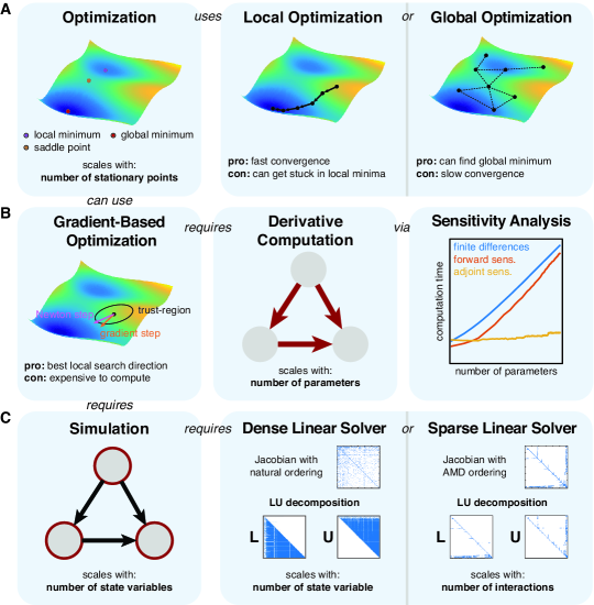
Figure 1: Overview of numerical methods and scaling properties for parameter inference. (A) Schematic scaling properties of optimization. Icons and properties of local and global optimizations are shown on the right. (B) Examples of gradient-based methods to determine parameter updates. Computation times of different approaches for gradient computation are shown on the right. (C) Schematic scaling properties of simulation algorithms. Dense and sparse direct linear solvers are compared on the right. Reordering was performed using the Approximative Minimum Degree (AMD) ordering algorithm Amestoy et al (1996)

Properties of the Optimization Problem

The optimization problem (5) is convex in $y_{i}(t_{j},\bm{\theta})$, but usually non-convex in $\bm{\theta}$. Thus, the objective function $J(\bm{\theta})$ can possess local minima and saddle points. Local minima can be problematic as optimization algorithms may get stuck, yielding a suboptimal agreement between experimental data and model simulation. Interestingly, recent literature suggests that saddle points might affect the efficiency of optimization more severely than local minima Dauphin et al (2014). For unconstrained problems, saddle points and local minima are both stationary points $\bm{\theta}^{*}$ at which the gradient vanishes

$$\nabla J(\bm{\theta}^{*})=0,$$ (9)

i.e., they both satisfy a necessary local optimality condition (see Figure 1A left for an example). The sufficient condition for a local minimum is the positive definiteness of the Hessian $\nabla^{2}J(\bm{\theta}^{*})$, which indicates that there are only directions of positive curvature. For a saddle point the Hessian $\nabla^{2}J(\bm{\theta}^{*})$ is indefinite or semi-definite, which indicates that there may be directions of negative or zero curvature.

The dependence of the number of local minima and saddle points for ODE models on the number of parameters is poorly understood. For deep learning problems, an exponential increase in the number of local minima with the number of parameters is primarily attributed to parameter permutation symmetries Anandkumar and Ge (2016), which are rare in ODE models. Yet, for deep learning problems, saddle points are also problematic as they affect the performance of local optimization methods Dauphin et al (2014). Arguments for an exponential increase in stationary points with the number of parameters are often based on random matrix theory Dauphin et al (2014) and rely on strong assumptions on the distribution of entries in the Hessian of the objective function $J(\bm{\theta})$. These assumptions have to be rigorously checked as they can lead to wrong conclusions, as shown for the stability of ODEs Kirk et al (2015). As the objective function $J(\bm{\theta})$ depends on the solution to an ODE, the validity of such assumptions is not evident and difficult to assess rigorously. For saddle points, we are not aware of any rigorous evaluation. Thus, the exact dependence of the number of local minima and saddle points on the parameter dimensionality remains elusive.

2.2 Optimization Methods

The infamous No Free Lunch Theorem for optimization Wolpert and Macready (1997) states that there exists no single optimization method that performs best on all classes of optimization problems. Accordingly, empirical evidence as well as a careful analysis of the problem structure should be considered when selecting a suitable optimization method. The plethora of different optimization methods commonly used in systems biology can be classified as

1. local and global methods, as well as

2. gradient-based and derivative-free methods.

Local methods search for local optima, while global methods search for global minima. The separation into local and global methods is often not clear-cut. Thus, methods, such as simulated annealing, are sometimes classified as local and sometimes as global methods Goffe et al (1994); Neumaier (2004); Johnson and McGeoch (1997). Therefore, the following paragraph contains many soft statements that should only serve as guidelines. Gradient-based methods exploit first and potentially higher order derivatives of the objective function, while derivative-free methods solely use the objective function.

Table 1: Examples for local and global, as well as derivative-free and gradient-based optimization algorithms

	Derivative-Free	Gradient-Based
	Pattern Search Hooke and Jeeves (1961)	Gradient Descent Nocedal and Wright (2006)
Local	Nelder-Mead Nelder and Mead (1965)	Newtons Method Nocedal and Wright (2006)
	Hill Climbing De La Maza and Yuret (1994)	Levenberg-Marquardt Levenberg (1944); Marquardt (1963)
	Genetic Algorithm Holland (1992)	Multi-Start Neumaier (2004)
Global	Particle Swarm Kennedy (2011)	Scatter Search Egea et al (2007)
	Simulated Annealing Kirkpatrick et al (1983)	Clustering Search Kan and Timmer (1987)

Local methods construct a sequence of trial points that successively decrease the objective function values (See Figure 1A middle). This procedure is usually faster than global methods, but can get stuck in local minima Ashyraliyev et al (2009). Most local derivative-free methods are direct search methods Hooke and Jeeves (1961). In contrast to local methods, global methods often rely on a population of trial points which are iteratively refined (see Figure  1A right). This can increase the chance of reaching the global minimum, but usually slower Ashyraliyev et al (2009). Global derivative-free methods mostly employ stochastic schemes, which are often inspired by nature Fister Jr et al (2013), while global gradient-based methods usually perform repeated local optimizations. Examples of local and global as well as respective derivative-free and gradient based methods are given in Table 1.

Not all global methods are guaranteed to converge to the global minimum Neumaier (2004). Convergence to the global minimum is only guaranteed for rigorous and (asymptotically) complete global methods, such as branch-and-bound Lawler and Wood (1966) and grid search Neumaier (2004). As long as only local information, i.e., function values and respective parameter derivatives, is available, the termination of these methods will require exponentially expensive dense search Neumaier (2004); Törn and Zilinskas (1989). The termination of global methods is crucial, as it might be relatively easy to find the global minimum but comparably hard to guarantee that it is indeed the global minimum. Global information, such as Lipschitz constants, is rarely available for ODE problems, such that dense, i.e., exhaustive, search would be necessary for guaranteed convergence. As the parameters $\bm{\theta}$ are generally continuous, dense search is rarely possible. Instead, meta-heuristics for termination and optimization are employed.

For many meta-heuristic methods, there exists little to no theoretical justification or convergence proofs Neumaier (2004). Others may converge with probability arbitrarily close to 1, but might only do so after infinitely many function evaluations. In practice, many meta-heuristic algorithms even fail to work reliably for smooth, convex problems with few parameters Rios and Sahinidis (2013). In fact, for some algorithms, non-convergence can even be proven mathematically Rudolph (1994). Eventually, even a rigorous convergence guarantee will be useless if the convergence rate is too slow for practical purposes. For most methods, there exists a plethora of disparate variants, which renders comprehensive analysis of convergence proofs and convergence rates challenging. This is quite unsatisfying from a theoretical perspective. In practice, reasonable results can be obtained using global optimization methods Moles et al (2003); Raue et al (2013); Banga (2008). Yet, usually no guarantees of global optimality can be given.

For the remainder of this chapter we will primarily focus on global gradient-based optimization methods, which typically rely on repeated local optimization. For these meta-heuristic methods, a local optimization is started at (random) points in parameter space. The termination of these methods usually relies on a specified maximum number of local optimizations, but also Bayesian methods can be applied Boender and Rinnooy Kan (1987). For the convergence to the global minimum, the local optimization has to be started in the region of attraction of the global optimum. Thus, the probability of convergence will depend on the relative volume of the region of attraction with respect to the search domain $\bm{\theta}$. Several adaptive methods, such as scatter search Egea et al (2007) or clustering search Kan and Timmer (1987), try to improve the chance of starting a local optimization in the region of attraction of the global optimum, but rely on the embeddedness of the global optimum Törn et al (1999). The embeddedness of the global optimum characterizes how well local minima cluster and determines how indicative the objective function value at the starting point is of the chance of converging to the global minimum. We are not aware of any analysis of embeddedness of the global minimum for models in systems biology, but it is likely to be problem dependent. The resulting rate of convergence will be determined by the rate of convergence of the local method and the probability to sample a starting point from the region of attraction of the global optimum.

For most methods that employ repeated local optimization, the individual local optimization runs can trivially be run in parallel Fröhlich et al (2017), which enables efficient use of high performance computing structure. Moreover, multiple global runs can be asynchronously parallelized to enhance efficiency through cooperativity Penas et al (2015). Following recent studies Raue et al (2013); Hross and Hasenauer (2016), we deem this repeated local optimization a suitable candidate for scalable optimization and will in the following discuss the properties of respective local gradient based methods (see Figure 1B) in more detail.

Line-Search Methods

Line-search methods are local optimization methods that iteratively update the parameter values in direction $\textbf{s}\in\mathbb{R}^{{n_{\theta}}}$, such that the objective function value $J(\bm{\theta})$ is successively reduced:

$$\bm{\theta}_{k}=\bm{\theta}_{k-1}+\gamma\cdot\textbf{s}\quad s.t.\quad J(\bm{\theta}_{k})<J(\bm{\theta}_{k-1}),\gamma>0,$$ (10)

where $\gamma\in\mathbb{R_{+}}$ controls the step size. For line-search, the update direction s is fixed first and then a suitable $\gamma$ is determined. The alternative to line-search methods are trust-region methods which first define a maximum step length and then find a suitable update direction. We will discuss trust-region methods in more detail in the following subsection. The classification in line-search or trust-region methods can be ambiguous and may depend on the specific implementation of the method. This will be discussed in more detail at the end of this subsection. In this chapter, we will follow the classification of Nocedal and Wright, who also provide an excellent discussion of the topic Nocedal and Wright (2006).

Line-search methods are particularly appealing as they reduce the possibly high-dimensional optimization problem to a sequence of one-dimensional problems of finding good values for $\gamma$. To ensure convergence, $\gamma$ has to meet certain conditions Armijo (1966); Wolfe (1969). Methods to determine the step size that satisfy these conditions are sometimes referred to as globalization techniques. Note that enforcing these conditions only guarantees convergence to a local stationary point, i.e., a local minimum, local maximum or saddle point, but not to a global minimum Nocedal and Wright (2006).

It is more or less well established that for local optimization, gradient-based methods should be used when applicable. Kolda et al. state in their review on direct search methods that "Today, most people’s first recommendation (including ours) to solve an unconstrained problem for which accurate first derivatives can be obtained would not be a direct search method, but rather a gradient-based method" Kolda et al (2003). Lewis et al. claim that "the success of quasi-Newton methods, when applicable, is now undisputed" Lewis et al (2000). Gradient-based methods, such as quasi-Newton methods, are applicable when the gradient (and the Hessian) of the objective function is continuous and can be computed accurately. By definition, the gradient $\nabla J(\bm{\theta})$ is only continuous with respect to parameters when the objective function is continuously differentiable. Higher order continuous differentiability corresponds to continuity of the respective higher order derivatives, such as the Hessian. For many noise distributions, such as the normal and log-normal distribution, the negative log-likelihood is infinitely often continuously differentiable with respect to the observables, given that a finite number of measurements is considered. Thus, the continuity of derivatives of the objective function (5) only depends on the continuity of derivatives of the model output (2). However, for particular noise distributions, such as the Laplace distribution, the negative log-likelihood may not be differentiable with respect to the model outputs. In the following, we will assume that both, (2) and (5), are twice continuously differentiable with respect to the parameters.

For continuously differentiable objective functions, an intuitive choice for s is the gradient

$$\textbf{s}_{\mathrm{grad}}=-\nabla J(\bm{\theta}_{k-1}).$$ (11)

Optimization methods using this search direction are called gradient descent methods. Locally, the gradient provides the steepest descent with respect to the euclidean norm. This means that the gradient points in the direction d, with unit length in the euclidean norm, which yields the strongest decrease of $J(\bm{\theta})$ in a neighborhood around $\bm{\theta}$:

$$\frac{\nabla J(\bm{\theta})}{\|\nabla J(\bm{\theta})\|_{2}}=\underset{\textbf{d}:\|\textbf{d}\|_{2}=1}{\mathrm{argmin}}\nabla J(\bm{\theta})^{T}\textbf{d}.$$ (12)

Yet, depending on the objective function, this neighborhood might be arbitrarily small, resulting in small values $\gamma$. This, for instance, is the case for objective functions with curved ridges, e.g., the Rosenbrock function Rosenbrock (1960), which can arise from (non-linear) dependencies between parameters. Moreover, gradient descent methods take small steps in the vicinity of saddle points Dauphin et al (2014), which can lead to high iteration numbers or premature termination in individual optimization runs.

The issue of small step sizes is addressed in the Newton’s method by including the Hessian $\nabla^{2}J(\bm{\theta}_{k-1})$, which encodes the curvature, in the calculation of the search direction s:

$$\textbf{s}_{\mathrm{newt}}=-\nabla^{2}J(\bm{\theta}_{k-1})^{-1}\nabla J(\bm{\theta}_{k-1}).$$ (13)

For the classical Newton’s method, the step size is fixed to $\gamma=1$. However, many modern implementations implement Newton’s method as line-search using 1 as default value and adapting the step size if necessary Nocedal and Wright (2006).

As the Hessian is symmetric, highly efficient methods such as Cholesky factorization can be used to solve this problem for convex optimization problems. However, for ODE models, the computation of the Hessian itself will usually be computationally far more expensive than the computation of the Newton step. Thus, the computational cost of solving (13) is usually negligible for objective functions depending on ODE models.

For non-convex problems, the computation of the Newton step  (13) may be an ill-posed or not even well-defined problem Nocedal and Wright (2006). Moreover, the Newton step might not be a descent direction. The Newton step is only a direction of descent if the scalar product with the gradient is negative:

$$\textbf{s}_{\mathrm{newt}}^{T}\cdot\nabla J(\bm{\theta}_{k-1})<0.$$ (14)

By substituting the formula for the Newton step, we obtain the following inequality:

$$-\nabla J(\bm{\theta}_{k-1})^{T}\left(\nabla^{2}J(\bm{\theta}_{k-1})\right)^{-1}\nabla J(\bm{\theta}_{k-1})<0,$$ (15)

which is globally satisfied only if the inverse of the Hessian $\nabla^{2}J(\bm{\theta}_{k-1})^{-1}$ is positive definite, i.e., the problem (6) is convex. As previously discussed, (6) is typically non-convex, thus simple Newton steps will not always yield a direction of descent. Moreover, in the vicinity of a saddle point, the Newton step may point in the direction of the saddle point, thus attracting the optimizer to saddle points Yuan (2015); Dauphin et al (2014).

In the literature, several modifications of Newton’s method that always yield descent directions have been proposed Levenberg (1944); Marquardt (1963); Hartley (1961). The Gauss-Newton Hartley (1961) method exploits the least-squares structure of the objective function (5) and constructs a positive semi-definite approximation to $\nabla^{2}J(\bm{\theta}_{k-1})$. Levenberg Levenberg (1944) and Marquardt Marquardt (1963) independently extended this method by introducing a dampening term in the step equation. This yields the Levenberg-Marquardt method

$$-(\bm{\hat{H}}(\bm{\theta}_{k-1})+\lambda\bm{I})\textbf{s}=\nabla J(\bm{\theta}_{k-1}),$$ (16)

where $\bm{\hat{H}}$ is the positive semi-definite Gauss-Newton approximation to the Hessian, $\lambda\geq 0$ is the dampening factor and $\bm{I}$ is the identity matrix. The magnitude of the dampening factor $\lambda$ regulates the conditioning of (16). The geometric interpretation of $\lambda$ is that it allows an interpolation between a gradient and a Gauss-Newton step, where $\lambda=0$ corresponds to a pure approximate Newton step. Due to the positive-definiteness of the Gauss-Newton approximation, the respective methods cannot follow directions of negative curvature and are thus not attracted to saddle points, but again limited to small step-sizes in the vicinity of saddle points Dauphin et al (2014).

As the Gauss-Newton method is limited to least-squares problems, the traditional formulation of the Levenberg-Marquardt method has the same limitation. However, it is possible to apply the dampening of the Hessian without the Gauss-Newton approximation. The resulting algorithms are often still referred to as Levenberg-Marquardt method Nesterov and Polyak (2006). In such a setting, the dampening is often chosen according to the smallest negative eigenvalue Nocedal and Wright (2006), using e.g., the Lanczos method Lanczos (1950), to ensure the construction of a direction of descent. In the vicinity of saddle points, these methods can be modified to also follow directions of negative curvature Nash (1984).

An alternative to determine the dampening factor $\lambda$ is the use of a trust-region method. A trust region method fixes $\|\gamma\bm{s}\|=\Delta$ and then determines an approximately matching $\lambda$ Nocedal and Wright (2006). Thus, Levenberg-Marquardt algorithms can be implemented as line-search methods or as trust-region methods, depending on how $\lambda$ and $\gamma$ are computed. In the following we will discuss trust-region methods more generally.

Trust-Region Methods

Line-search methods determine a search direction $d$ first and then identify a good step size $\gamma$. Trust region methods do the converse, by specifying a maximum step-size first and then identifing a good search direction Byrd et al (1987); Sorensen (1982); Nocedal and Wright (2006). This allows trust region methods to make large steps close to saddle points and always yield descent directions. Within the trust-region, $J(\bm{\theta})$ is replaced by a local approximation, giving rise to the trust-region subproblem. Most trust-region algorithms use the objective function derivatives to construct a quadratic trust-region subproblem

$$\underset{\textbf{s}\in B_{\textbf{D},\Delta}(\bm{\theta})}{\min}\,\frac{1}{2}\textbf{s}^{T}\nabla^{2}J(\bm{\theta})\textbf{s}+\textbf{s}^{T}\nabla J(\bm{\theta}),$$ (17)

where $B_{\textbf{D},\Delta}(\bm{\theta})=\{\textbf{s}:\left\|\textbf{D}(\textbf{s}-\bm{\theta})\right\|_{2}\leq\Delta\}$ is the trust region. The trust region is an ellipsoid with radius $\Delta$ and scaling matrix D around the current parameter $\bm{\theta}$. The size of the trust region can be adapted over the course of iterations. Trust-region methods that do not use quadratic approximations use other local approximations, e.g., via radial basis functions Wild et al (2008).

Trust-region methods that solve the subproblem (17) exactly are not attracted to saddle points and not limited to small step sizes Dauphin et al (2014). However, the quadratic problem (17) is usually difficult to solve exactly and is approximatively solved instead Nocedal and Wright (2006). For convex problems, the dogleg method Steihaug (1983), which employs a linear combination of gradient and Newton step, can be applied. For non-convex problems, the two-dimensional subspace minimization method Byrd et al (1988); Branch et al (1999) can be used. The two-dimensional subspace minimization method dampens the Hessian and can be seen as a trust-region variant of the Levenberg-Marquardt method. The dogleg and two-dimensional subspace minimization method both reduce the trust-region subproblem to a two dimensional problem, which renders the computational cost of determining the update step from a given gradient per se independent of the number of parameters of the underlying problem. This feature makes them particularly suited for large-scale problems. However, the dampening of the Hessian can again lead to small step-sizes close to saddle points Dauphin et al (2014).

Table 2: Implementations and interfaces of of optimization methods in popular computational biology toolboxes. Some toolboxes may feature variants of the cited algorithms. Some entries may be names of functions that feature multiple different algorithms.

Toolbox	Global	Local
		Derivative-Free	Gradient-Based
COPASI Hoops et al (2006)	Evolutionary Programming Fogel et al (1991)	Nelder Mead Nelder and Mead (1965)	Levenberg-Marquardt  Levenberg (1944); Marquardt (1963)
	Genetic Algorithm Michalewicz (2013)	Pattern Search Hooke and Jeeves (1961)	Steepest Descent Nocedal and Wright (2006)
	Particle Swarm Kennedy (2011)	PRAXIS Brent (2013)	Truncated Newton Dembo and Steihaug (1983)
	Random Search Solis and Wets (1981)
	Simulated Annealing  Kirkpatrick et al (1983)
	Scatter Search Egea et al (2007)
	SRES Runarsson and Yao (2000)
D2D Raue et al (2015)	fminsearchbnd (MATLAB)		arNLS (custom)
	Genetic Algorithm (MATLAB)		CERES (Google)
	multi-start (custom)		fmincon (MATLAB)
	Pattern Search (MATLAB)		lsqnonlin (MATLAB)
	Particle Swarm (custom)		STRSCNE Bellavia et al (2004)
	Simulated Annealing (MATLAB)		TRESNEI Morini and Porcelli (2012)
MEIGO Egea et al (2014)	fminsearchbnd (MATLAB)	DHC De La Maza and Yuret (1994)	fmincon (MATLAB)
	NOMAD Le Digabel (2011)	Pattern Search Kelley (1999)	IpOpt Wächter and Biegler (2006)
	multi-start(custom)	SOLNP Ye (1989)	lsqnonlin (MATLAB)
	Scatter Search Egea et al (2007)		MISQP Exler et al (2012)
			N2FB Dennis et al (1981)
			NL2SOL Dennis et al (1981)
PESTO Stapor et al (2018)	multi-start (custom)	BOBYQA Powell (2009)	fmincon (MATLAB)
	Particle Swarm Vaz and Vicente (2009)	DHC De La Maza and Yuret (1994)	lsqnonlin (MATLAB)
	MEIGO Egea et al (2014)

Implementation and Practical Considerations

State-of-the-art parameter inference toolboxes for computational biology, such as D2D Raue et al (2015), PESTO Stapor et al (2018), MEIGO Egea et al (2014) and COPASI Hoops et al (2006), feature a mix of local and global methods which include derivative-free and gradient-based methods (see Table 2). In terms of global, derivative-free methods, most toolboxes provide interfaces to Particle Swarm and Pattern Search methods. In terms of local, gradient-based methods, most toolboxes feature various flavors of the trust-region algorithm. All MATLAB toolboxes provide interfaces to the fmincon and lsqnonlin routines from the MATLAB Optimization Toolbox. Only COPASI provides the implementation of more basic algorithms such as Levenberg-Marquardt Levenberg (1944); Marquardt (1963), Truncated Newton and Steepest Descent. In terms of global optimization schemes, all toolboxes employ either multi-start or scatter search algorithms Egea et al (2007).

Choosing a particular optimization method from this plethora of choices is not an easy task. There are no exhaustive studies that compare the full range of different optimization methods on a large set of problems. In some studies, gradient-based optimization algorithms perform best Raue et al (2013); Hross and Hasenauer (2016), but others also show that derivative-free methods can perform well Degasperi et al (2017). In general, a rigorous evaluation of optimization algorithms is highly involved, as there are small differences in the implementations of various algorithms. For example, STRSCNE Bellavia et al (2004), RESNEI Morini and Porcelli (2012), NL2SOL Dennis et al (1981), lsqnonlin and fmincon all implement trust-region algorithms and even for expert users it may be difficult to pinpoint differences between individual implementations. A recent study suggests substantial differences in the efficiency of various implementations of trust-region algorithms and identified lsqnonlin to be the best performing algorithm Wieland (2016). Even for a single implementation the specification of hyper-parameters can have substantial impact on performance. Many algorithms require user specifications of technical parameters. Finding good values for these hyper-parameters may be challenging for non-expert users and default values may not work for all problems.

As few researchers are experts in a large number of different optimization methods, a rigorous evaluation of multiple different algorithms is challenging. To circumvent this problem, a recent study Villaverde et al (2015) suggested a set of benchmark problems on which other researchers are invited to evaluate their algorithms. Yet, few algorithms have been evaluated on that benchmark so far Penas et al (2015); Fröhlich et al (2017). Complementarily, (Kreutz, 2016) suggests the construction of statistical models to assess the performance of methods and the effect of hyper-parameters.

The different optimization algorithms we outlined in this section rely on evaluations of the objective function, its gradient or even its Hessian. In the following sections we will the discuss methods to evaluate these terms.

2.3 Simulation

The objective function and its gradient are typically not available in closed form, but have to be computed numerically. For large-scale models the computational cost of computing the objective function and its gradient is high, which makes parameter estimation computationally demanding. Depending on the class of the employed model and simulation algorithm, the computation time will depend on different features of the underlying model, which we will discuss in detail in the following.

The timescales of biochemical processes span multiple orders of magnitude Shamir et al (2016); Hasenauer et al (2015). As comprehensive models often cover a large variety of different biological processes, they are particularly prone to possess multiple timescales Smallbone and Mendes (2013). This results in the stiffness of corresponding ODEs Resat et al (2009). As the stiffness of the equations typically depends on the choice of parameters, it is rarely possible to assess the stiffness a priori. Consequently, it is always advisable to use implicit solvers, which can adequately handle stiffness, for parameter inference Gonnet et al (2012).

Implicit Methods

For stiff problems, implicit differential equation solvers from the fully implicit Runge-Kutta solver family Butcher (1964), the Singly Diagonally Implicit Runge-Kutta solver family Alexander (1977) or the Rosenbrock solver family Rosenbrock (1963) should be used. These solvers compute the state variables at the next time step $\xi_{i}$ based on the state variables at previous iterations $x(\xi_{i-1}),x(\xi_{i-2}),x(\xi_{i-3}),\ldots$ by solving an implicit equation

$$G(\textbf{x}(\xi_{i}),\textbf{x}(\xi_{i-1}),\textbf{x}(\xi_{i-2}),\textbf{x}(\xi_{i-3}),\ldots)=0,$$

where the function $G$ depends on the choice of the method and on the right hand side of the differential equation $f$.

For single-step methods, such as the Runge-Kutta type solvers, the function $G$ will only depend on $x(\xi_{i-1})$, and not on previous values. For implicit Runge-Kutta solvers, a system of linear equations with ${n_{x}}\cdot s$ equations has to be solved in every iteration Zhang and Sandu (2014). Here $s$ is a the number of stages, which is a particular property of a Runge-Kutta solver which determines the order of the method.

For multi-step methods, the function $G$ will also depend on previous values of x. A popular implementation of the multi-step method is the implicit linear multi-step Backwards Differentiation Formula (BDF) implemented in the CVODES solver Serban and Hindmarsh (2005). In every iteration $i$, the BDF solves an equation of the form

$$h_{i}\beta_{i,0}f(\xi_{i},\textbf{x}(\xi_{i}),\bm{\theta})+\sum_{j=0}^{q}\alpha_{i,j}\textbf{x}(\xi_{i-j})=0,$$

where $q$ is the order of the method, $\bm{\alpha}$ and $\bm{\beta}$ are the coefficients that are determined in every iteration. The order $q$ and the step size $h_{i}$ will determine the local error of the numerical solution Serban and Hindmarsh (2005) and are often chosen adaptively. This implicit equation is typically solved using Newton’s method Hindmarsh et al (2005); Zhang and Sandu (2014). For the BDF, the function $G$ depends on $\dot{x}$ and thus on $f$. Consequently, the Newton solver computes multiple solutions to linear systems defined by the Jacobian $\nabla_{x}f(t,\textbf{x},\bm{\theta})$ of the right hand side of the differential equation at every integration step. As this linear system only has ${n_{x}}$ equations, in contrast to the ${n_{x}}\cdot s$ equations for single-step methods, the computational cost of solving the linear system increases less strongly with the number of state variables ${n_{x}}$.

The computation time of the BDF method primarily depends on two factors: (i) the evaluation time of the function $f$ and the Jacobian $\nabla_{x}f(t,\textbf{x},\bm{\theta})$, which usually scales linearly with ${n_{x}}$ and (ii) the time to solve the linear systems defined by $\nabla_{x}f(t,\textbf{x},\bm{\theta})$. The matrix $\nabla_{x}f(t,\textbf{x},\bm{\theta})$ is typically not symmetric and neither positive nor negative definite. For such unstructured problems, LU decomposition (see Figure 1C middle), which factorizes $\nabla_{x}f(t,\textbf{x},\bm{\theta})$ into a lower-triangular matrix L and an upper-triangular matrix U, is the method of choice to solve the linear system, as long as L and U can be stored in memory. After performing the decomposition, the solution to the linear systems can be computed by matrix multiplication. When no additional structure of the matrix is exploited, the computational complexity of matrix multiplication with state-of-the-art algorithms increases at least with exponent $2.376$ with respect to ${n_{x}}$ Coppersmith and Winograd (1990) and thus dominates the computation time for sufficiently large ${n_{x}}$.

Sparse Implicit Methods

For ODE models arising from discretization of partial differential equations, the Jacobian can usually be brought into banded form. For such banded matrices, specialized solvers that scale with the number of off-diagonals of the Jacobian have been developed Thorson (1979). Unfortunately, ODE models of biochemical reaction networks cannot generally be brought into a banded structure. For example, in polymerization reactions that include dissociation of monomers, the monomer species will always be influenced by all other species and the number of off-diagonals in the Jacobian will be equal to ${n_{x}}$. Other frequently occurring motifs, such as feedback loops and single highly interactive species Barabasi and Oltvai (2004), will also increase the number of necessary off-diagonals.

As alternative to banded solvers, sparse solvers have been introduced in the context of circuit simulations Davis and Palamadai Natarajan (2010). For sparse solvers, the computation time depends on the number of non-zero entries in $\nabla_{x}f(t,x,\bm{\theta})$, which scales with the number of biochemical reactions. The sparse solver relies on an approximate minimum degree (AMD) ordering Amestoy et al (1996) which is a graph theoretical approach that can be used to minimize the fill-in of the L and U matrices of the LU-decomposition (see  1C right). Currently, no formulas for the expected speedup or the general scaling with respect to non-zero entries exist. For biochemical reaction networks, the application of such a sparse solver seems reasonable Gonnet et al (2012), but no rigorous evaluation of the scaling has been performed.

Implementation and Practical Considerations

Most toolboxes use CVODES Serban and Hindmarsh (2005) or LSODA Petzold (1983) for simulation (see Table 3). In contrast to CVODES, which only implements an implicit solver, LSODA dynamically switches between explicit and implicit solvers. To the best of our knowledge, no comparison between LSODA and CVODES has ever been published. However, LSODA does not provide an interface to the Clark Kent LU solver (KLU) Davis and Palamadai Natarajan (2010) or any other sparse solver and thus might perform poorly on large-scale problems with sparsity structure. Another notable difference is that only few toolboxes analytically compute the Jacobian of the right hand side and provide it to the solver. The symbolic processing is necessary for the sparse representation, but also likely to be beneficial for dense solvers. Thus, D2D Raue et al (2015) and AMICI Fröhlich et al (2017) are also the only general purpose simulation libraries for systems biology that allow the use of the sparse KLU solver.

For explicit solvers, no linear system has to be solved and the algorithm largely consists of elementary operations which can be efficiently parallelized on GPUs Tangherloni et al (2017). For explicit solvers, also parallelized solvers are available Demmel et al (1999). However, the computational overhead of parallelization is usually too high, unless models with several thousand state variables are considered Demmel et al (1999).

All of the considered toolboxes allow the definition of ODE models in the Systems Biology Markup Language (SBML) Hucka et al (2003). This also allows for the definition of models in terms of biochemical reactions. Here COPASI and libRoadRunner aim for a full support of SBML features, while AMICI and D2D only support a subset of SBML features.

Table 3: Implementations of simulation methods in popular computational biology toolboxes.

Toolbox	Simulation Library	Jacobian	Dense Solver	Sparse Solver
AMICI Fröhlich et al (2017)	CVODES Serban and Hindmarsh (2005)	symbolic
COPASI Hoops et al (2006)	LSODA Petzold (1983)	numeric		$\times$
D2D Raue et al (2015)	CVODES Serban and Hindmarsh (2005)	symbolic
libRoadRunner Somogyi et al (2015)	CVODES Serban and Hindmarsh (2005)	numeric		$\times$

Sparse numerical solvers can be used to efficiently compute the numerical solution to the ODE, which are required for objective function evaluation. They can also be used to compute objective function gradients as solution to one or more ODEs. Several different gradient computation approaches exist and in the following we will discuss the three most common approaches.

2.4 Gradient Calculation

Providing an accurate gradient to the objective function is essential for gradient-based methods Raue et al (2013); Griewank and Walther (2008); Nocedal and Wright (2006). For ODE constrained optimization problems, the gradient of the objective function can be computed based on the parametric derivative of the solution to the ODE. These derivatives are often called the sensitivities of the model. Several approaches to compute sensitivities for ODE models exist, including finite differences Milne-Thompson (1933), as well as the direct approach via forward sensitivity analysis Dickinson and Gelinas (1976); Kokotovic and Heller (1967).

Finite Differences and Forward Sensitivity Analysis

For finite differences, the entries of the gradient are approximated according to

$$\frac{\mathrm{d}J}{\mathrm{d}\theta_{k}}\approx\frac{J(\bm{\theta}+a\,\textbf{e}_{k})-J(\bm{\theta}-b\,\textbf{e}_{k})}{a+b},$$

with $a,b\geq 0$ and the $k^{th}$ unit vector $\textbf{e}_{k}$. In practice, forward differences ($a=\zeta$, $b=0$), backward differences ($a=0$, $b=\zeta$) and central differences ($a=\zeta$, $b=\epsilon$), with $\zeta\ll 1$, are widely used. As the evaluation of $J(\bm{\theta}+a\,\textbf{e}_{k})$ and $J(\bm{\theta}-b\,\textbf{e}_{k})$ may require additional solutions to the model ODE, the scaling of finite differences with respect to the number of parameters is also linear.

For forward sensitivity analysis, the entries of the gradient of the objective function are computed according to

$$\frac{\mathrm{d}J}{\mathrm{d}\theta_{k}}=-\sum_{i=1}^{n_{y}}\sum_{j=1}^{T}\frac{\partial J}{\partial y_{i}(t_{j},\theta)}s_{i,k}^{y}(t_{j},\bm{\theta})+\frac{\partial J}{\partial\theta_{k}},$$

with $s_{i,k}^{y}(t,\bm{\theta})$ denoting the sensitivity of output $y_{i}$ at time point $t_{j}$ with respect to parameter $\theta_{k}$. This output sensitivity can be computed by applying the total derivative to the functions $h$:

$$s^{y}_{i,k}(t_{j},\bm{\theta})=\left.\frac{\partial h_{i}}{\partial x}\right|_{\textbf{x}(t,\bm{\theta}),\bm{\theta}}s^{x}_{k}(t_{j},\bm{\theta})+\left.\frac{\partial h_{i}}{\partial\theta_{k}}\right|_{x(t,\bm{\theta}),\bm{\theta}}$$

with $\textbf{s}^{x}_{k}(t,\bm{\theta})$ denoting the sensitivity of the state x with respect to $\theta_{k}$. The state sensitivity is defined as solution to the ODE system:

$$\dot{\textbf{s}}^{x}_{k}(t,\bm{\theta})=\left.\frac{\partial f}{\partial x}\right|_{x(t,\bm{\theta}),\bm{\theta}}\textbf{s}^{x}_{k}(t,\bm{\theta})+\left.\frac{\partial f}{\partial\theta_{k}}\right|_{x(t,\bm{\theta}),\bm{\theta}},\qquad\textbf{s}^{x}_{k}(t_{0},\bm{\theta})=\left.\frac{\partial x_{0}}{\partial\theta_{k}}\right|_{\bm{\theta}}.$$

Thus, forward sensitivity analysis requires the computation of a solution to an ODE system of the same size as the model ODE for every gradient entry. Consequently, the scaling with respect to the number of parameters is linear (see Figure 1B right).

Adjoint Sensitivity Analysis

The linear scaling of forward sensitivity analysis and finite differences can be computationally prohibitively demanding for large-scale models with thousands of parameters. The alternative adjoint approach, which computes the objective function gradient via adjoint sensitivity analysis, has long been deemed to be computationally more efficient for systems with many parameters Kokotovic and Heller (1967). In other research fields, e.g., for partial differential equation constrained optimization problems, adjoint sensitivity analysis Hindmarsh et al (2005) has been adopted in the past decades. In contrast, in the systems biology community there are only isolated applications of adjoint sensitivity analysis Lu et al (2008); Fujarewicz et al (2005); Lu et al (2012).

In the mathematics and engineering community, adjoint sensitivity analysis is frequently used to compute the gradients of a functional with respect to the parameters if the functional depends on the solution of a differential equation Plessix (2006). In these applications, measurements are continuous in time and $J(\bm{\theta})$ is assumed to be a functional of the solution $\textbf{x}(t)$ of a differential equation. However, this approach can also be applied to discrete-time measurements and in contrast to forward sensitivity analysis, adjoint sensitivity analysis does not rely on the state sensitivities $\textbf{s}^{x}_{k}(t)$, but on the adjoint state $\textbf{p}(t)$.

For discrete-time measurements – the usual case in systems and computational biology – the adjoint state is piece-wise continuous in time and defined by a sequence of backward differential equations Fröhlich et al (2017). For $t>t_{N}$, the adjoint state is zero, $\textbf{p}(t)=0$. Starting from this end value, the trajectory of the adjoint state is calculated backwards in time, from the last measurement $t=t_{N}$ to the initial time $t=t_{0}$. At the measurement time points $t_{N},\ldots,t_{1}$, the adjoint state is reinitialized as

$$\textbf{p}(t_{j})=\lim_{t\rightarrow t_{j}^{+}}\textbf{p}(t)+\frac{\partial J}{\partial x},$$ (18)

which usually results in a discontinuity of $p(t)$ at $t_{j}$. Starting from the end value $p(t_{j})$ as defined in (18) the adjoint state evolves backwards in time until the next measurement point $t_{j-1}$ or the initial time $t_{0}$ is reached. This evolution is governed by the time dependent linear ODE

$$\dot{\textbf{p}}=-\left(\frac{\partial f}{\partial x}\right)^{T}\textbf{p}.$$ (19)

The repeated evaluation of (18) and (19) until $t=t_{0}$ yields the trajectory of the adjoint state. Given this trajectory, the gradient of the objective function with respect to the individual parameters is

$$\frac{\mathrm{d}J}{\mathrm{d}\theta_{k}}=-\int_{t_{0}}^{t_{N}}\textbf{p}^{T}\frac{\partial f}{\partial\theta_{k}}dt-\textbf{p}(t_{0})^{T}\frac{\partial\textbf{x}_{0}}{\partial\theta_{k}}+\frac{\partial J}{\partial\theta_{k}}.$$ (20)

The key advantage of this approach is that (20), which has to be evaluated for every parameter separately, can be evaluated very efficiently, while (19), which is computationally more demanding, only has to be solved once Fröhlich et al (2017). As (19) is of the same dimensionality as the original ODE model, this allows the computation of gradients at the cost of roughly two solutions of the original ODE model. In practice the adjoint sensitivity approach has an almost constant scaling with respect to the number of parameters.

Implementation and Practical Considerations

Many toolboxes rely on finite differences to compute gradients (see Table 4). D2D Raue et al (2015) and AMICI Fröhlich et al (2017) are two notable examples that allow the computation of gradients via sensitivity analysis, but only AMICI allows adjoint sensitivity analysis.

Table 4: Implementations of gradient computation methods in popular computational biology toolboxes.

Toolbox	Finite Differences	Forward Sensitivity	Adjoint Sensitivity
AMICI Fröhlich et al (2017)	$\times$
COPASI Hoops et al (2006)		$\times$	$\times$
D2D Raue et al (2015)			$\times$
libRoadRunner Somogyi et al (2015)		$\times$	$\times$

2.5 Hessian Computation

In addition to the gradient, Newton-type methods also require the Hessian $\nabla^{2}J(\bm{\theta})$ of the objective function. The numerical evaluation of the Hessian can be challenging as the dependence of the computational complexity on the number of parameters ${n_{\theta}}$ is one order higher than for the gradient: The computation time for finite differences and forward sensitivities scale quadratically with the number of parameters Balsa-Canto et al (2001); Vassiliadis et al (1999). For adjoint sensitivities, the computation time depends linearly on the number of parameters Özyurt and Barton (2005).

Gauss-Newton Approximation

For independent, normally distributed measurement noise, as assumed in (5), and known noise parameters $\sigma$, the optimization problem (6) is of least squares type. This structure can be exploited by using Gauss-Newton (GN) Björck (1996) type algorithms, which ignore second order partial derivatives in the Hessian. The respective approximations of the Hessian coincide with the Fisher information matrix (FIM) Fisher (1922) of the respective parameter estimate. The key advantage of this approach is that the FIM can be computed for the same cost as one gradient using forward sensitivity analysis.

Quasi-Newton Approximation

For problems that are not of least-squares type, quasi-Newton methods such as the Broyden-Fletcher-Goldfarb-Shanno (BFGS) Fletcher and Powell (1963); Goldfarb (1970) algorithm can be used. The BFGS algorithm iteratively computes approximations to the Hessian based on updates which are derived from the outer products of the gradient $\nabla J(\bm{\theta})$ of the objective function. The resulting approximation is guaranteed to be positive definite, as long as the Wolfe condition Wolfe (1969) is satisfied in every iteration and the initial approximation is positive definite. As previously discussed, positive definiteness ensures descent directions for line-search methods, but will generally lead to small step sizes in the vicinity of saddle points. The symmetric rank 1 (SR1) algorithm addresses this problem by allowing for negative- and indefinite approximations Byrd et al (1996). This procedure facilitates the application of optimization methods which avoid saddle points by allowing directions of negative curvature Ramamurthy and Duffy (2017).

Quasi-Newton versions are generally cheap to compute, as they only require simple algebraic manipulations of the gradient. Algorithms based on limited memory variants such as L-BFGS Nocedal (1980); Liu and Nocedal (1989) or L-SR1 Ramamurthy and Duffy (2017) have been applied to machine learning problems with millions of parameters Andrew and Gao (2007).

Implementation and Practical Considerations

Table 5: Implementations of (approximative) Hessian computation methods in popular computational biology toolboxes. For BFGS and SR1 we list the function or option that allows the respective approximation. SE = sensitivity equations, FD = finite differences, GN = Gauss-Newton, N/A = Not applicable

Toolbox	FIM / GN	Hessian	BFGS	SR1
AMICI Fröhlich et al (2017)	SE	SE	N/A	N/A
COPASI Hoops et al (2006)	FD	$\times$	Truncated Newton	$\times$
D2D Raue et al (2015)	SE/FD	$\times$	fmincon	arNLS_SR1
libRoadRunner Somogyi et al (2015)	$\times$	$\times$	N/A	N/A
MEIGO Hoops et al (2006)	N/A	N/A	fmincon, IpOpt	IpOpt
PESTO Stapor et al (2018)	N/A	N/A	fmincon	$\times$

The implementation of methods for the computation of (approximate) Hessians is quite disparate across toolboxes (see Table 5). AMICI is the only toolbox that allows sensitivity-based computation of the Hessian. Most other toolboxes use FIM/Gauss-Newton, BFGS or SR1 approximations. Most of iterative approximations BFGS and SR1 are implemented as part of the optimization algorithm and it is not possible to use them with other methods. Only D2D provides a relatively flexible implementation of SR1. For the FIM approximation and the exact Hessian computations, the implementations are usually transferable between optimization methods. In theory, the computation of the exact Hessian, with adjoint sensitivity analysis, and the FIM, with forward sensitivity analysis, both scale linearly with the number of parameters and only the exact Hessian can be used to construct methods that avoid saddle points Dauphin et al (2014). In practice, the effect of using the FIM over the Hessian on the efficiency of respective optimization methods has not been studied for systems biology problems. For problems with thousands of parameters, the computation of both may be challenging and the BFGS and SR1 approximations become more appealing.

In this section, we split the parameter inference problem in three parts: optimization, simulation and gradient computation and discussed respective scaling properties. These techniques generalize to other model analysis techniques that require optimization or gradient computation, such as uncertainty analysis Raue et al (2009); Girolami and Calderhead (2011), experimental design Vanlier et al (2012) and the inference of model structure. A detailed discussion of all these methods is beyond the scope of this book chapter, but in the following we will discuss the inference of model structure in more detail.

3 Inference of Model Structure

In many applications, it is not apparent which biochemical species and reactions are necessary to describe the dynamics of a biochemical process. In this case, the structure of the ODE model (1), i.e., vector field $f(\textbf{x},\bm{\theta})$ and initial condition $\textbf{x}_{0}(\bm{\theta})$, have to be inferred from experimental data. The selection should compromise between goodness-of-fit and complexity. Following the concept of Occam’s razor Blumer et al (1987), one tries to control variability associated with over-fitting while protecting against the bias associated with under-fitting.

In the following, we formulate the problem of model structure inference. We introduce and discuss criteria that select models out of a set of candidate models and describe approaches to reduce the number of candidate models. We outline the scalability of the approaches and their computational complexity.

3.1 Model Selection Criteria

Given a set of candidate models $M_{1},M_{2},\ldots,M_{{n_{M}}}$ the aim of model inference is to find a model or a set of models which (i) describe the data available and (ii) generalize to other datasets Hastie et al (2009). The choice of model can be made with several selection criteria, differing among others in asymptotic consistency Shibata (1980), asymptotic efficiency Fisher (1922) and computational complexity. If the true model is included in the set of candidate models, a consistent criterion will asymptotically select the true model with probability one and an efficient criterion will select the model that minimizes the mean squared error of the prediction.

While the concepts in the previous sections followed the frequentist approach, some of the concepts presented in this section are Bayesian. For these approaches, prior knowledge about the parameters is incorporated and the posterior probability (7) is analyzed instead of the likelihood function.

One popular criterion is the Bayes factor Kass and Raftery (1995), which has been shown to be asymptotically consistent for a broad range of models (e.g., Wang and Sun (2014); Choi and Rousseau (2015)), however, for the case of general ODE models, no proofs for asymptotic efficiency and consistency are available for all the criteria presented in this section. Bayes’ Theorem yields the posterior model probability

$$p(M_{m}|\mathcal{D})=\frac{p(\mathcal{D}|M_{m})p(M_{m})}{p(\mathcal{D})}$$ (21)

with marginal likelihood

$$p(\mathcal{D}|M_{m})=\int_{\Theta_{m}}p(\mathcal{D}|\bm{\theta}_{m})p(\theta_{m}|M_{m})d\bm{\theta}_{m}$$ (22)

with model prior $p(M_{m})$ and marginal probability $p(\mathcal{D})=\sum_{j}p(\mathcal{D}|M_{j})P(M_{j})$. The Bayes factor of models $M_{1}$ and $M_{2}$ is the ratio of the corresponding marginal likelihoods

$$B_{12}=\frac{p(\mathcal{D}|{M}_{1})}{p(\mathcal{D}|{M}_{2})}.$$ (23)

The Bayes factor describes how much more likely it is that the data are generated from $M_{1}$ instead of $M_{2}$. A Bayes factor $B_{12}>100$ is often considered decisive for rejecting model ${M}_{2}$ Jeffreys (1961). The Bayes factor intrinsically penalizes model complexity by integrating over the whole parameter space of each model. Bayes factors can be approximated by Laplace approximation, which has a low computational complexity but provides only a local approximation. To enable a more precise computation of the Bayes factors, bridge sampling Meng and Wong (1996), nested sampling Skilling (2006), thermodynamic integration Hug et al (2016), or related methods can be employed. These approaches evaluate the integral defining the marginal likelihood $p(\mathcal{D}|M_{m})$. As the approaches require a large-number of function evaluations, the methods are usually computationally demanding and the computational complexity is highly problem-dependent. Thus, efficient sampling methods are required.

For high-dimensional or computationally demanding problems, the calculation of Bayes factors might be intractable and computationally less expensive model selection criteria need to be employed. A model selection criterion which is based on the MLE, instead of a marginal likelihood (an integral over the whole parameter space), is the Bayesian Information Criterion (BIC) Schwarz (1978). The BIC value for model $M_{m}$ is

$$\mathrm{BIC}_{m} =-2\log\left(p\left(\mathcal{D}|\bm{\theta}_{m}^{*}\right)\right)+\log\left(|\mathcal{D}|\right){n_{\theta_{m}}}\,.$$ (24)

For structural identifiable models, the BIC provides in the limit of large sample sizes information about the Bayes factors,

$$\lim_{|\mathcal{D}|->\infty}\frac{-2\log B_{12}-(\mathrm{BIC}_{1}-\mathrm{BIC}_{2})}{-2\log B_{12}}=0\,.$$ (25)

From information theoretical arguments, the Akaike Information Criterion (AIC)

$$\mathrm{AIC}_{m} =-2\log\left(p\left(\mathcal{D}|\bm{\theta}_{m}^{*}\right)\right)+2{n_{\theta_{m}}}\,,$$ (26)

has been derived Akaike (1973). Low BIC and AIC values are preferable and differences above $10$ are assumed to be substantial (see Table 6 and Kass and Raftery (1995); Burnham and Anderson (2002)).

For model selection in many problem classes, the AIC is asymptotically efficient, but not consistent, while the BIC is asymptotically consistent, but not efficient Shibata (1981); Kuha (2004); Acquah (2010).

Table 6: Decisions based on the Bayes factor and differences in BIC and AIC values Jeffreys (1961); Kass and Raftery (1995); Burnham and Anderson (2002).

Blm	$\mathrm{BIC}_{m}-\min_{l}\mathrm{BIC}_{l}$	$\mathrm{AIC}_{m}-\min_{l}\mathrm{AIC}_{l}$	decision
$1-3$	$0-2$	$0-4$	do not reject model $M_{m}$
$3-100$	$2-10$	$4-10$	-
$>100$	$>10$	$>10$	reject model $M_{m}$

When incorporating prior information about parameters, the priors can conceptually be treated as additional data points and, thus, be part of the likelihood to still allow the use of BIC and AIC. Also extensions of the criteria exist, such as the corrected AIC Hurvich and Tsia (1989), which provides a correction for finite sample sizes. Also other extended versions of the criteria have been developed (see, e.g., Chen and Chen (2008)), however, the discussion of these is beyond the scope of this chapter.

For the comparison of nested models $M_{m}$ and $M_{l}$ , i.e., $\bm{\theta}_{m}\in\Theta_{m}$ and $\bm{\theta}_{l}\in\Theta_{l}$ where $\Theta_{m}$ is a subset of $\Theta_{l}$, the likelihood ratio test can be applied Wilks (1938), which is an efficient test Neyman and Pearson (1992). The likelihood ratio is defined as

$$\Lambda=\frac{p(\mathcal{D}|\bm{\theta}_{m}^{*})}{p(\mathcal{D}|\bm{\theta}_{l}^{*})}\leq 1\,,$$ (27)

and model $M_{m}$ is rejected if $\Lambda$ is below a certain threshold which is obtained using Wilks’ Theorem Wilks (1938). This theorem states that it holds in the large sample limit (see Wilks (1938) for further details)

$$2(\log p(\mathcal{D}|\bm{\theta}_{l}^{*})-\log p(\mathcal{D}|\bm{\theta}_{m}^{*}))\sim\chi^{2}(\cdot|{n_{\theta_{l}}}-{n_{\theta_{m}}}).$$ (28)

Given a certain $\alpha$ level, model $M_{m}$ is rejected if

$$\int_{0}^{2(\log p(\mathcal{D}|\bm{\theta}_{l}^{*})-\log p(\mathcal{D}|\bm{\theta}_{m}^{*}))}\chi^{2}(\psi|{n_{\theta_{l}}}-{n_{\theta_{m}}})d\psi\geq 1-\alpha\,.$$ (29)

While only Bayes factors and the likelihood ratio test are proven to be valid for non-identifiable parameters, the use of AIC and BIC can be problematic for these cases.

The discussion of further criteria, such as the log-pointwise predictive density Gelman et al (2014) or cross-validation (see, e.g., Arlot and Celisse (2010)), which evaluate the predictive quality of the model, is beyond the scope of this chapter.

Implementation and Practical Considerations

AIC and BIC are rather simple to compute and are, among others, available in PESTO Stapor et al (2018). From the previously discussed toolboxes of this review, PESTO also provides sampling methods that can be employed to calculate Bayes factors, such as parallel tempering. Other toolboxes which can be employed for computing Bayes factors are, amongst others, BioBayes Vyshemirsky and Girolami (2008), MultiNest Feroz et al (2009), or the C++ toolbox BCM Thijssen et al (2016).

3.2 Reduction of Number of Models

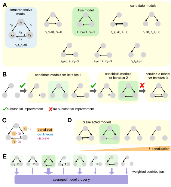
Figure 2: Illustration of methods for model reduction. (A) Set of candidate models, varying in the existence of connections between nodes $x_{1},x_{2}$ and $x_{3}$. In total, there are $2^{{n_{r}}}=2^{3}$ models with at least ${n_{\eta}}=1$ parameters. (B) Illustration of forward-selection starting from minimal model. In the first iteration, the model with $r_{1}\neq 0,r_{2},r_{3}=0$ is selected (green) and in the second iteration the model with $r_{1},r_{3}\neq 0,r_{2}=0$. The full model is rejected based on the selection criteria. (C) To apply $l_{0}$ penalization a MINLP problem needs to be solved, comprising continuous parameters $\bm{\eta}$ and $\mathbf{r}$ and discrete parameters $\textbf{q}\in\{0,1\}^{{n_{r}}}$. (D) $l_{1}$ penalization reduces the number of potential models to a set of preselected models by increasing the penalization and thus forcing parameters $r$ to zero. (E) Illustration of model averaging. The thickness of the arrows corresponds to the posterior probability, Akaike weight, or BIC weight and indicates the contribution of the model to the averaged model properties.

For most models, computing Bayes’ factors is computationally demanding compared to optimization and the evaluation of AIC, BIC, or likelihood ratio. Yet, if the number of candidate models ${n_{M}}$ is large, even the evaluation of AIC and BIC can become limiting as ${n_{M}}$ optimization problems have to be solved. For non-nested models, the model selection criterion of choice needs to be calculated for each model to determine the optimal model.

In this section, we consider a nested set of candidate models. In this case, all candidate models are a special case of a comprehensive model and can be constructed by fixing a subset of the parameters to specific values (Figure 2A). For the remainder of this chapter, we will assume that we can split the model parameters $\bm{\theta}$ into general parameters $\bm{\eta}\in\mathbb{R}^{{n_{\eta}}}$, which are present in all models, and difference parameters $\mathbf{r}\in\mathbb{R}^{{n_{r}}}$, which encode the nesting between models. Moreover, without loss of generality, it is assumed that $r_{i}=0,i=1,\ldots,{n_{r}}$ corresponds to the simplest model and $r_{i}\neq 0,i=1,\ldots,{n_{r}}$ corresponds to the most complex model (see Figure 2A). These difference parameters could for example be the kinetic rates of hypothesized reactions Klimovskaia et al (2016) or scaling factors for possibly cell-type or condition-specific parameters (see, e.g., Steiert et al (2016)). Such settings yield a total of $2^{{n_{r}}}$ candidate models, where ${n_{r}}$ is limited by ${n_{\theta}}$. Thus, for models with a high number of parameters, also a high number of nested models is possible. When ${n_{r}}$ and ${n_{\theta}}$ are both high, the inference of model parameters and thus the inference of model structure is challenging.

Forward-Selection and Backward-Elimination

In statistics, step-wise regression is an often-used approach to reduce the number of models that need to be tested. This comprises forward-selection and backward-elimination (e.g., Hastie et al (2009)) and combinations of both Kaltenbacher and Offtermatt (2011). Forward-selection is a bottom-up approach which starts with the least complex model and successively activates individual difference parameters (i.e., setting $r_{i}\neq 0$) until a sufficient agreement with experimental data is achieved, evaluated using a model selection criterion (Figure 2B). In contrast, backward-elimination is a top-down approach starting with the most complex model, successively deactivating individual difference parameters (i.e., setting $r_{i}=0$) that are not required for a good fit to the data.

Forward-selection and backward-elimination reduce the number of models that need to be compared with the model selection criteria described before from $2^{{n_{r}}}$ to at most $\frac{n_{r}(n_{r}+1)}{2}$. However, they are both greedy approaches and do not guarantee to find the globally least complex candidate model that explains the data.

$l_{0}$ Penalized Objective Function

An alternative approach is to penalize the number of parameters in the objective function. This can be achieved by imposing an $l_{0}$ penalization on the objective function (see, e.g.,  Liu and Li (2016)):

$$J_{l_{0}}(\bm{\eta},\mathbf{r})=J(\bm{\eta},\mathbf{r})+\lambda\left({{n_{\eta}}}+\sum_{i=1}^{{n_{r}}}\left(1-\delta_{r_{i}}\right)\right),\qquad\mbox{with\leavevmode\nobreak\ }\delta_{z}=\begin{cases}1\;\mathrm{if}\;z=0\\ 0\;\mathrm{otherwise}\end{cases}$$ (30)

This $l_{0}$ penalization supports sparsity, i.e., reduces the model such that only a minimum number of difference parameters are used. As all models contain at least ${n_{\eta}}$ parameters, only ${n_{r}}$ contributes to changes in the complexity. For $\lambda=1$, the objective function $J_{l_{0}}$ is the AIC divided by two. For $\lambda=\frac{1}{2}\log\left(|\mathcal{D}|\right)$, the objective function $J_{l_{0}}$ is the BIC divided by two. Accordingly, minimization of $J_{l_{0}}$ can provide the best model according to different information criteria. To directly assess the predictive power, $\lambda$ can also be determined using cross-validation.

Following Rodriguez-Fernandez et al (2013), the objective function (30) allows for the formulation of structure inference as a mixed-integer nonlinear programming (MINLP) problem

$$J_{MINLP}(\bm{\eta},\mathbf{r},\mathbf{q})=J(\bm{\eta},\mathrm{diag}(\mathbf{r}\mathbf{q}^{T}))+\lambda\sum_{i=1}^{{n_{r}}}q_{i},$$ (31)

with real-valued $\bm{\eta}\in\mathbb{R}^{{n_{\eta}}},\mathbf{r}\in\mathbb{R}^{{n_{r}}}$, and integer-valued $\mathbf{q}\in\{0,1\}^{{n_{r}}}$. The optimization is done simultaneously for all parameters, $\bm{\eta},\mathbf{r},\mathbf{q}$. This objective function is neither differentiable, nor continuous with respect to $\mathbf{q}$. Thus, gradients with respect to the discrete parameters will not be informative for optimization. This limits the choice of optimization algorithms to derivative-free and specialized gradient-based solvers, such as the MISQP algorithm Henriques et al (2015). Besides the above described and commonly used methods, further approaches, among others belief propagation Molinelli et al (2013) or iteratively reweighted least squares Daubechies et al (2010) can be employed, under certain model assumptions.

For the MINLP (31) resulting from the $l_{0}$ penalized objective functions, only the comprehensive model is estimated. This, however, results in a more complex optimization problem which suffers from a high dimensional parameter space.

$l_{1}$ Penalized Objective Function

To simplify the optimization problem, the $l_{0}$ norm is often replaced by its convex relaxation, the $l_{1}$ norm Tibshirani (1996). This yields the penalized objective function

$$J_{l_{1}}(\bm{\eta},\mathbf{r})=J(\bm{\eta},\mathbf{r})+\lambda\sum_{i=1}^{{n_{r}}}|r_{i}|,$$ (32)

with $r_{i}\in\mathbb{R}$, which is forced to be zero for higher $\lambda$ corresponding to the situations where the parameter $\theta_{i}$ has no effect. In linear regression, $l_{1}$ penalization is more commonly known as Lasso Tibshirani (1996), while in signal processing it is usually referred to as Basis Pursuit Chen et al (2001). The $l_{1}$ norm is continuous, but not differentiable in zero. Thus, specialized solvers have been developed which handle the non-differentiability at zero Steiert et al (2016).

For the special case of linear regression models $J_{l_{0}}(\bm{\eta},\mathbf{r})$ and $J(\bm{\eta},\mathbf{r})$ are convex. As the $l_{1}$ norm is a convex relaxation of the $l_{0}$ norm, the resulting objective function is also convex. Thus, it can be shown that the estimated parameters $r_{i}$ are unique and continuous with respect to $\lambda$ Efron et al (2004). Moreover, $r_{i}$ can be shown to be piecewise linear with respect to $\lambda$, which allows an implementation that can efficiently compute solutions for all values of $\lambda$ Efron et al (2004). For ODE models, $J_{l_{1}}(\bm{\eta},\mathbf{r})$ and $J(\bm{\eta},\mathbf{r})$ will generally be non-convex and $r_{i}$ may be non-unique and discontinuous which is challenging for numerical methods. Thus, equation (32) is usually minimized for varying penalization strengths $\lambda$, until a reduced set of model candidates is selected. As the $l_{1}$ norm is an approximation of the $l_{0}$ norm, model selection should subsequently be performed on the reduced set of model candidates using the criteria introduced in Section 3.1 (Figure 2D).

The computational complexity of the $l_{1}$ penalization depends on the number of different penalization strengths that are used. With a higher number of tested penalizations it is more likely to obtain the globally optimal model, while a lower number of tested penalizations decreases the computational effort.

Implementation and Practical Considerations

Only few toolboxes implement methods that allow simultaneous inference of model parameters and structure. MEIGO implements the MISQP algorithm, while D2D implements the $l_{1}$ penalization via a modification of the fmincon routine Steiert et al (2016).

3.3 Model Averaging

For large sets of candidate models and limited data, it frequently happens that not a single model is chosen by the model selection criterion. Instead, a set of models is plausible, cannot be rejected, and should be considered in the subsequent analysis. In this case, model averaging can be employed to predict the behaviour of the process (Figure 2E).

Given that a certain parameter is comparable between models, an average estimate can be derived as

$$\mathbb{E}[\theta_{j}]=\sum_{m}w_{m}\theta_{m,j}$$ (33)

with $w_{m}$ denoting the weight of model $M_{m}$ and $\theta_{m,j}$ denoting the MLE of the parameter for model $M_{m}$ Wassermann (2000); Burnham and Anderson (2002). Accordingly, uncertainties can be evaluated, e.g., the variance of the optimal values

$$\mathrm{var}[\theta_{j}]=\frac{1}{{n_{M}}-1}\sum_{m}(w_{m}\theta_{m,j}-\mathbb{E}[\theta_{j}])^{2}.$$ (34)

The weights capture the plausibility of the model. An obvious choice is the posterior probability $p({M}_{m}|\mathcal{D})$. Alternatively, the Akaike weights

$$w_{m}=\frac{\exp(-\frac{1}{2}\mathrm{AIC}_{m})}{\sum_{i=1}^{{n_{M}}}\exp(-\frac{1}{2}\mathrm{AIC}_{i})}$$ (35)

or the BIC weights

$$w_{m}=\frac{\exp(-\frac{1}{2}\mathrm{BIC}_{m})}{\sum_{i=1}^{{n_{M}}}\exp(-\frac{1}{2}\mathrm{BIC}_{i})}.$$ (36)

can be employed. The weights for models that are not plausible are close to zero and, thus, these models do not influence the averaged model.

4 Discussion

This chapter provided an overview about methods for parameter inference and structure inference for ODE models of biochemical systems. For parameter inference we discussed local optimization methods and identified the number of stationary points as key determinant of computational complexity. In the context of local optimization we identified gradient-based optimization methods as suitable method as the computational complexity of determining the parameter update for optimization from the gradient of the objective function is per se independent of the number of state variables and number of model parameters. Still, numerical optimization requires the computation of the ODE solution, which scales with the number of molecular species, and the computation of respective derivatives, which scales with the number of parameters. In both cases we discussed scaling properties of state-of-art algorithms and identified adjoint sensitivity analysis and sparse solvers as most suitable methods for large-scale problems.

We believe that key challenges to improve the scalability of parameter inference lie in the treatment of stationary points of the objective function, such as local minima and saddle points. In contrast to deep learning problems Dauphin et al (2014), the dependence of the number of stationary points on the underlying (ODE) model remains poorly understood Mannakee et al (2016); Transtrum et al (2011) and should be evaluated. Local optimization methods that can account for saddle points and local minima have been developed Kan and Timmer (1987); Neumaier (2004); Dauphin et al (2014), but lack implementations in computational biology toolboxes and evaluations on ODE models of biochemical systems.

For structure inference, large-scale models often also give rise to a large set of different model candidates. Many model comparison criteria require parameter inference for all model candidates, which is rarely feasible if the number of model candidates is high. We discussed an $l_{1}$ penalization based approach that allows the simultaneous inference of model parameters and structure. We believe that key challenges to improve the scalability of structure inference lie in the treatment of non-differentiability of the $l_{1}$ norm, which prohibits the application of standard gradient-based optimization algorithms. Methods such as iteratively reweighted least-squares were developed decades ago Holland and Welsch (1977), but were not adopted for ODE models.

We anticipate that, with the advent of whole cell models Karr et al (2012); Babtie and Stumpf (2017); Tomita et al (1999) and other large-scale models Fröhlich et al (2017); Büchel et al (2013), the demand for scalable methods will drastically increase in the coming years. However, already for medium-scale models, which are much more commonplace, parameter inference and in particular structure inference can be challenging. Accordingly, there is a growing demand for novel methods with better scaling properties.

References

- Klipp et al (2005) Klipp E, Herwig R, Kowald A, Wierling C, Lehrach H (2005) Systems biology in practice. Wiley-VCH, Weinheim
- Kitano (2002a) Kitano H (2002a) Systems biology: A brief overview. Science 295(5560):1662–1664
- Kitano (2002b) Kitano H (2002b) Computational systems biology. Nature 420(6912):206–210
- Adlung et al (2017) Adlung L, Kar S, Wagner MC, She B, Chakraborty S, Bao J, Lattermann S, Boerries M, Busch H, Wuchter P, Ho AD, Timmer J, Schilling M, Höfer T, Klingmüller U (2017) Protein abundance of AKT and ERK pathway components governs cell type-specific regulation of proliferation. Mol Syst Biol 13(1):904, DOI 10.15252/msb.20167258
- Buchholz et al (2013) Buchholz VR, Flossdorf M, Hensel I, Kretschmer L, Weissbrich B, Gräf P, Verschoor A, Schiemann M, Höfer T, Busch DH (2013) Disparate individual fates compose robust CD8+ T cell immunity. Science 340(6132):630–635, DOI 10.1126/science.1235454
- Intosalmi et al (2016) Intosalmi J, Nousiainen K, Ahlfors H, Läähdesmäki H (2016) Data-driven mechanistic analysis method to reveal dynamically evolving regulatory networks. Bioinformatics 32(12):i288–i296, DOI 10.1093/bioinformatics/btw274
- Hug et al (2016) Hug S, Schwarzfischer M, Hasenauer J, Marr C, Theis FJ (2016) An adaptive scheduling scheme for calculating Bayes factors with thermodynamic integration using Simpson’s rule. Stat Comput 26(3):663–677, DOI 10.1007/s11222-015-9550-0
- Hross et al (2016) Hross S, Fiedler A, Theis FJ, Hasenauer J (2016) Quantitative comparison of competing PDE models for Pom1p dynamics in fission yeast. In: Findeisen R, Bullinger E, Balsa-Canto E, Bernaerts K (eds) Proc. 6th IFAC Conf. Found. Syst. Biol. Eng., IFAC-PapersOnLine, vol 49, pp 264–269, DOI 10.1016/j.ifacol.2016.12.136
- Toni et al (2012) Toni T, Ozaki Yi, Kirk P, Kuroda S, Stumpf MPH (2012) Elucidating the in vivo phosphorylation dynamics of the ERK MAP kinase using quantitative proteomics data and Bayesian model selection. Mol Biosyst 8:1921–1929, DOI 10.1039/C2MB05493K
- Molinelli et al (2013) Molinelli EJ, Korkut A, Wang W, Miller ML, Gauthier NP, Jing X, Kaushik P, He Q, Mills G, Solit DB, Pratilas CA, Weigt M, Braunstein A, Pagnani A, Zecchina R, Sander C (2013) Perturbation biology: Inferring signaling networks in cellular systems. PLoS Comput Biol 9(12):e1003,290, DOI 10.1371/journal.pcbi.1003290
- Schilling et al (2009) Schilling M, Maiwald T, Hengl S, Winter D, Kreutz C, Kolch W, Lehmann WD, Timmer J, Klingmüller U (2009) Theoretical and experimental analysis links isoformspecific ERK signalling to cell fate decisions. Mol Syst Biol 5(334)
- Fey et al (2015) Fey D, Halasz M, Dreidax D, Kennedy SP, Hastings JF, Rauch N, Munoz AG, Pilkington R, Fischer M, Westermann F, Kolch W, Kholodenko BN, Croucher DR (2015) Signaling pathway models as biomarkers: Patient-specific simulations of JNK activity predict the survival of neuroblastoma patients. Sci Signal 8(408), DOI 10.1126/scisignal.aab0990
- Eduati et al (2017) Eduati F, Doldàn-Martelli V, Klinger B, Cokelaer T, Sieber A, Kogera F, Dorel M, Garnett MJ, Blüthgen N, Saez-Rodriguez J (2017) Drug resistance mechanisms in colorectal cancer dissected with cell type-specific dynamic logic models. Cancer Res 77(12):3364–3375, DOI 10.1158/0008-5472.CAN-17-0078
- Hass et al (2017) Hass H, Masson K, Wohlgemuth S, Paragas V, Allen JE, Sevecka M, Pace E, Timmer J, Stelling J, MacBeath G, Schoeberl B, Raue A (2017) Predicting ligand-dependent tumors from multi-dimensional signaling features. npj Syst Biol Appl 3(1):27, DOI 10.1038/s41540-017-0030-3
- Maiwald et al (2016) Maiwald T, Hass H, Steiert B, Vanlier J, Engesser R, Raue A, Kipkeew F, Bock HH, Kaschek D, Kreutz C, Timmer J (2016) Driving the model to its limit: Profile likelihood based model reduction. PLoS ONE 11(9), DOI 10.1371/journal.pone.0162366
- Snowden et al (2017) Snowden TJ, van der Graaf PH, Tindall MJ (2017) Methods of model reduction for large-scale biological systems: A survey of current methods and trends. B Math Biol 79(7):1449–1486, DOI 10.1007/s11538-017-0277-2
- Transtrum and Qiu (2016) Transtrum MK, Qiu P (2016) Bridging mechanistic and phenomenological models of complex biological systems. PLoS Comput Biol 12(5):1–34, DOI 10.1371/journal.pcbi.1004915
- Dano et al (2006) Dano S, Madsen MF, Schmidt H, Cedersund G (2006) Reduction of a biochemical model with preservation of its basic dynamic properties. FEBS Journal 273(21):4862–4877, DOI 10.1111/j.1742-4658.2006.05485.x
- Klonowski (1983) Klonowski W (1983) Simplifying principles for chemical and enzyme reaction kinetics. Biophys Chem 18(2):73–87, DOI 10.1016/0301-4622(83)85001-7
- Hoops et al (2006) Hoops S, Sahle S, Gauges R, Lee C, Pahle J, Simus N, Singhal M, Xu L, Mendes P, Kummer U (2006) COPASI – a COmplex PAthway SImulator. Bioinformatics 22(24):3067–3074, DOI 10.1093/bioinformatics/btl485
- Raue et al (2015) Raue A, Steiert B, Schelker M, Kreutz C, Maiwald T, Hass H, Vanlier J, Tönsing C, Adlung L, Engesser R, Mader W, Heinemann T, Hasenauer J, Schilling M, Höfer T, Klipp E, Theis FJ, Klingmüller U, Schöberl B, JTimmer (2015) Data2Dynamics: a modeling environment tailored to parameter estimation in dynamical systems. Bioinformatics 31(21):3558–3560, DOI 10.1093/bioinformatics/btv405
- Somogyi et al (2015) Somogyi ET, Bouteiller JM, Glazier JA, König M, Medley JK, Swat MH, Sauro HM (2015) libRoadRunner: A high performance SBML simulation and analysis library. Bioinformatics 31(20):3315–3321, DOI 10.1093/bioinformatics/btv363
- Santos et al (2007) Santos SDM, Verveer PJ, Bastiaens PIH (2007) Growth factor-induced MAPK network topology shapes Erk response determining PC-12 cell fate. Nat Cell Biol 9(3):324–330, DOI 10.1038/ncb1543
- Yao et al (2016) Yao J, Pilko A, Wollman R (2016) Distinct cellular states determine calcium signaling response. Mol Syst Biol 12(12):894, DOI 10.15252/msb.20167137
- Ogilvie et al (2017) Ogilvie LA, Kovachev A, Wierling C, Lange BMH, Lehrach H (2017) Models of models: A translational route for cancer treatment and drug development. Frontiers in Oncology 7:219, DOI 10.3389/fonc.2017.00219
- Schillings et al (2015) Schillings C, Sunnåker M, Stelling J, Schwab C (2015) Efficient characterization of parametric uncertainty of complex (bio)chemical networks. PLoS Comput Biol 11(8):e1004,457, DOI 10.1371/journal.pcbi.1004457
- Babtie and Stumpf (2017) Babtie AC, Stumpf MPH (2017) How to deal with parameters for whole-cell modelling. J R Soc Interface 14(133), DOI 10.1098/rsif.2017.0237
- Ocone et al (2015) Ocone A, Haghverdi L, Mueller NS, Theis FJ (2015) Reconstructing gene regulatory dynamics from high-dimensional single-cell snapshot data. Bioinformatics 31(12):i89–i96, DOI 10.1093/bioinformatics/btv257
- Kondofersky et al (2015) Kondofersky I, Fuchs C, Theis FJ (2015) Identifying latent dynamic components in biological systems. IET Syst Biol 9(5):193–203
- Akaike (1973) Akaike H (1973) Information theory and an extension of the maximum likelihood principle. In: 2nd International Symposium on Information Theory, Tsahkadsor, Armenian SSR, Akademiai Kiado, vol 1, pp 267–281
- Schwarz (1978) Schwarz G (1978) Estimating the dimension of a model. Ann Statist 6(2):461–464, DOI 10.1214/aos/1176344136
- Steiert et al (2016) Steiert B, Timmer J, Kreutz C (2016) L1 regularization facilitates detection of cell type-specific parameters in dynamical systems. Bioinformatics 32(17):i718–i726, DOI 10.1093/bioinformatics/btw461
- Klimovskaia et al (2016) Klimovskaia A, Ganscha S, Claassen M (2016) Sparse regression based structure learning of stochastic reaction networks from single cell snapshot time series. PLoS Comput Biol 12(12):e1005,234, DOI 10.1371/journal.pcbi.1005234
- Loos et al (2017) Loos C, Moeller K, Fröhlich F, Hucho T, Hasenauer J (2017) Mechanistic hierarchical population model identifies latent causes of cell-to-cell variability. bioRxiv DOI 10.1101/171561
- Hock et al (2013) Hock S, Hasenauer J, Theis FJ (2013) Modeling of 2D diffusion processes based on microscopy data: Parameter estimation and practical identifiability analysis. BMC Bioinf 14(Suppl 10)(S7), DOI 10.1186/1471-2105-14-S10-S7
- Hross (2016) Hross S (2016) Parameter estimation and uncertainty quantification for image based systems biology. Ph.D. thesis, Technische Universität München
- Menshykau et al (2013) Menshykau D, Germann P, Lemereux L, Iber D (2013) Simulating organogenesis in COMSOL: Parameter optimization for PDE-based models. In: Proceedings of COMSOL Conference, Rotterdam, Netherlands
- Hross and Hasenauer (2016) Hross S, Hasenauer J (2016) Analysis of CFSE time-series data using division-, age- and label-structured population models. Bioinformatics 32(15):2321–2329, DOI 10.1093/bioinformatics/btw131
- Fröhlich et al (2016) Fröhlich F, Thomas P, Kazeroonian A, Theis FJ, Grima R, Hasenauer J (2016) Inference for stochastic chemical kinetics using moment equations and system size expansion. PLoS Comput Biol 12(7):e1005,030, DOI 10.1371/journal.pcbi.1005030
- Ruess and Lygeros (2015) Ruess J, Lygeros J (2015) Moment-based methods for parameter inference and experiment design for stochastic biochemical reaction networks. ACM T Math Softwares Model Comput S 25(2):8, DOI 10.1145/2688906
- Munsky et al (2009) Munsky B, Trinh B, Khammash M (2009) Listening to the noise: random fluctuations reveal gene network parameters. Mol Syst Biol 5(318), DOI 10.1038/msb.2009.75
- Kreutz et al (2007) Kreutz C, Bartolome Rodriguez MM, Maiwald T, Seidl M, Blum HE, Mohr L, Timmer J (2007) An error model for protein quantification. Bioinformatics 23(20):2747–2753, DOI 10.1093/bioinformatics/btm397
- Maier et al (2017) Maier C, Loos C, Hasenauer J (2017) Robust parameter estimation for dynamical systems from outlier-corrupted data. Bioinformatics 33(5):718–725, DOI 10.1093/bioinformatics/btw703
- Puga et al (2015) Puga JL, Krzywinski M, Altman N (2015) Bayes’ theorem. Nat Methods 12(3):277–278, DOI 10.1038/nmeth.3335
- Amestoy et al (1996) Amestoy PR, Davis TA, Duff IS (1996) An approximate minimum degree ordering algorithm. SIAM J Matrix Anal A 17(4):886–905, DOI 10.1137/s0895479894278952
- Dauphin et al (2014) Dauphin YN, Pascanu R, Gulcehre C, Cho K (2014) Identifying and attacking the saddle point problem in high-dimensional non-convex optimization. In: Advances in Neural Information Processing Systems 26 (NIPS 2014), pp 2933–2941
- Anandkumar and Ge (2016) Anandkumar A, Ge R (2016) Efficient approaches for escaping higher order saddle points in non-convex optimization. In: Conference on Learning Theory, pp 81–102
- Kirk et al (2015) Kirk P, Rolando DM, MacLean AL, Stumpf MP (2015) Conditional random matrix ensembles and the stability of dynamical systems. New J Phys 17(8):083,025, DOI 10.1088/1367-2630/17/8/083025
- Wolpert and Macready (1997) Wolpert DH, Macready WG (1997) No free lunch theorems for optimization. IEEE Trans Evol Comput 1(1):67–82, DOI 10.1109/4235.585893
- Goffe et al (1994) Goffe WL, Ferrier GD, Rogers J (1994) Global optimization of statistical functions with simulated annealing. J Econometrics 60(1-2):65–99, DOI 10.1016/0304-4076(94)90038-8
- Neumaier (2004) Neumaier A (2004) Complete search in continuous global optimization and constraint satisfaction. Acta Numer 13:271–369, DOI 10.1017/s0962492904000194
- Johnson and McGeoch (1997) Johnson DS, McGeoch LA (1997) The traveling salesman problem: A case study in local optimization. Local search in combinatorial optimization 1:215–310
- Hooke and Jeeves (1961) Hooke R, Jeeves TA (1961) “Direct Search” solution of numerical and statistical problems. J ACM 8(2):212–229, DOI 10.1145/321062.321069
- Nocedal and Wright (2006) Nocedal J, Wright S (2006) Numerical Optimization. Springer Science & Business Media, DOI 10.1007/b98874
- Nelder and Mead (1965) Nelder JA, Mead R (1965) A simplex method for function minimization. Comput J 7(4):308–313, DOI 10.1093/comjnl/7.4.308
- De La Maza and Yuret (1994) De La Maza M, Yuret D (1994) Dynamic hill climbing. AI expert 9:26–26
- Levenberg (1944) Levenberg K (1944) A method for the solution of certain non-linear problems in least squares. Q Appl Math 2(2):164–168, DOI 10.1090/qam/10666
- Marquardt (1963) Marquardt DW (1963) An algorithm for least-squares estimation of non-linear parameters. SIAM J Appl Math 11(22):431–441, DOI 10.1137/0111030
- Holland (1992) Holland JH (1992) Adaptation in natural and artificial systems: an introductory analysis with applications to biology, control, and artificial intelligence. MIT press
- Kennedy (2011) Kennedy J (2011) Particle swarm optimization. In: Encyclopedia of machine learning, Springer, pp 760–766
- Egea et al (2007) Egea JA, Rodriguez-Fernandez M, Banga JR, Marti R (2007) Scatter search for chemical and bio-process optimization. J Global Optim 37(3):481–503, DOI 10.1007/s10898-006-9075-3
- Kirkpatrick et al (1983) Kirkpatrick S, Gelatt Jr CD, M P Vecchi MP (1983) Optimization by simulated annealing. Science 220(4598):671–680, DOI 10.1126/science.220.4598.671
- Kan and Timmer (1987) Kan AR, Timmer GT (1987) Stochastic global optimization methods part I: Clustering methods. Math Program 39(1):27–56, DOI 10.1007/BF02592070
- Ashyraliyev et al (2009) Ashyraliyev M, Fomekong-Nanfack Y, Kaandorp JA, Blom JG (2009) Systems biology: Parameter estimation for biochemical models. FEBS Journal 276(4):886–902, DOI 10.1111/j.1742-4658.2008.06844.x
- Fister Jr et al (2013) Fister Jr I, Yang XS, Fister I, Brest J, Fister D (2013) A brief review of nature-inspired algorithms for optimization. Elektrotehniski Vestnik 80(3):116–122
- Lawler and Wood (1966) Lawler EL, Wood DE (1966) Branch-and-bound methods: A survey. Oper Res 14(4):699–719, DOI 10.1287/opre.14.4.699
- Törn and Zilinskas (1989) Törn A, Zilinskas A (1989) Global Optimization, Lecture Notes in Computer Science, vol 350. Springer-Verlag, Berlin
- Rios and Sahinidis (2013) Rios LM, Sahinidis NV (2013) Derivative-free optimization: A review of algorithms and comparison of software implementations. J Global Optim 56(3):1247–1293, DOI 10.1007/s10898-012-9951-y
- Rudolph (1994) Rudolph G (1994) Convergence analysis of canonical genetic algorithms. IEEE transactions on neural networks 5(1):96–101, DOI 10.1109/72.265964
- Moles et al (2003) Moles CG, Mendes P, Banga JR (2003) Parameter estimation in biochemical pathways: A comparison of global optimization methods. Genome Res 13:2467–2474, DOI 10.1101/gr.1262503
- Raue et al (2013) Raue A, Schilling M, Bachmann J, Matteson A, Schelke M, Kaschek D, Hug S, Kreutz C, Harms BD, Theis FJ, Klingmüller U, Timmer J (2013) Lessons learned from quantitative dynamical modeling in systems biology. PLoS ONE 8(9):e74,335, DOI 10.1371/journal.pone.0074335
- Banga (2008) Banga JR (2008) Optimization in computational systems biology. BMC Syst Biol 2(47), DOI 10.1186/1752-0509-2-47
- Boender and Rinnooy Kan (1987) Boender CGE, Rinnooy Kan AHG (1987) Bayesian stopping rules for multistart global optimization methods. Math Program 37(1):59–80, DOI 10.1007/BF02591684
- Törn et al (1999) Törn A, Ali MM, Viitanen S (1999) Stochastic global optimization: Problem classes and solution techniques. J Global Optim 14(4):437–447, DOI 10.1023/A:1008395408187
- Fröhlich et al (2017) Fröhlich F, Kaltenbacher B, Theis FJ, Hasenauer J (2017) Scalable parameter estimation for genome-scale biochemical reaction networks. PLoS Comput Biol 13(1):e1005,331, DOI 10.1371/journal.pcbi.1005331
- Penas et al (2015) Penas DR, González P, Egea JA, Banga JR, Doallo R (2015) Parallel metaheuristics in computational biology: An asynchronous cooperative enhanced scatter search method. Procedia Comput Sci 51:630–639, DOI 10.1016/j.procs.2015.05.331
- Armijo (1966) Armijo L (1966) Minimization of functions having Lipschitz continuous first partial derivatives. Pac J Math 16(1):1–3, DOI 10.2140/pjm.1966.16.1
- Wolfe (1969) Wolfe P (1969) Convergence conditions for ascent methods. SIAM Rev 11(2):226–235, DOI 10.1137/1011036
- Kolda et al (2003) Kolda TG, Lewis RM, Torczon V (2003) Optimization by direct search: New perspectives on some classical and modern methods. SIAM Rev 45(3):385–482, DOI 10.1137/s003614450242889
- Lewis et al (2000) Lewis RM, Torczon V, Trosset MW (2000) Direct search methods: Then and now. J Comput Appl Math 124(1):191–207, DOI 10.1016/s0377-0427(00)00423-4
- Rosenbrock (1960) Rosenbrock HH (1960) An automatic method for finding the greatest or least value of a function. Comput J 3(3):175–184, DOI 10.1093/comjnl/3.3.175
- Yuan (2015) Yuan Yx (2015) Recent advances in trust region algorithms. Math Program 151(1):249–281
- Hartley (1961) Hartley HO (1961) The modified Gauss-Newton method for the fitting of non-linear regression functions by least squares. Technometrics 3(2):269–280, DOI 10.1080/00401706.1961.10489945
- Nesterov and Polyak (2006) Nesterov Y, Polyak B (2006) Cubic regularization of newton method and its global performance. Math Program 108(1):177–205, DOI 10.1007/s10107-006-0706-8
- Lanczos (1950) Lanczos C (1950) An iteration method for the solution of the eigenvalue problem of linear differential and integral operators. United States Governm. Press Office Los Angeles, CA, DOI 10.1137/1.9781611971187
- Nash (1984) Nash SG (1984) Newton-type minimization via the Lanczos method. SIAM Journal on Numerical Analysis 21(4):770–788, DOI 10.1137/0721052
- Byrd et al (1987) Byrd RH, Schnabel RB, Shultz GA (1987) A trust region algorithm for nonlinearly constrained optimization. SIAM J Numer Anal 24(5):1152–1170, DOI 10.1137/0724076
- Sorensen (1982) Sorensen DC (1982) Newton’s method with a model trust region modification. SIAM J Numer Anal 19(2):409–426, DOI 10.1137/0719026
- Wild et al (2008) Wild SM, Regis RG, Shoemaker CA (2008) ORBIT: Optimization by radial basis function interpolation in trust-regions. SIAM J Sci Comput 30(6):3197–3219, DOI 10.1137/070691814
- Steihaug (1983) Steihaug T (1983) The conjugate gradient method and trust regions in large scale optimization. SIAM Journal on Numerical Analysis 20(3):626–637, DOI 10.1137/0720042
- Byrd et al (1988) Byrd RH, Schnabel RB, Shultz GA (1988) Approximate solution of the trust region problem by minimization over two-dimensional subspaces. Math Program 40(1):247–263, DOI 10.1007/bf01580735
- Branch et al (1999) Branch MA, Coleman TF, Li Y (1999) A subspace, interior, and conjugate gradient method for large-scale bound-constrained minimization problems. SIAM J Sci Comput 21(1):1–23, DOI 10.1137/s1064827595289108
- Fogel et al (1991) Fogel DB, Fogel LJ, Atmar JW (1991) Meta-evolutionary programming. In: Signals, systems and computers, 1991. 1991 Conference record of the twenty-fifth asilomar conference on, IEEE, pp 540–545, DOI 10.1109/acssc.1991.186507
- Michalewicz (2013) Michalewicz Z (2013) Genetic Algorithms + Data Structures = Evolution Programs. Springer Science & Business Media
- Brent (2013) Brent RP (2013) Algorithms for minimization without derivatives. Courier Corporation
- Dembo and Steihaug (1983) Dembo RS, Steihaug T (1983) Truncated-newtono algorithms for large-scale unconstrained optimization. Math Program 26(2):190–212, DOI 10.1007/bf02592055
- Solis and Wets (1981) Solis FJ, Wets RJB (1981) Minimization by random search techniques. Math Oper Res 6(1):19–30, DOI 10.1287/moor.6.1.19
- Runarsson and Yao (2000) Runarsson TP, Yao X (2000) Stochastic ranking for constrained evolutionary optimization. IEEE T Evolut Comput 4(3):284–294, DOI 10.1109/4235.873238
- Bellavia et al (2004) Bellavia S, Macconi M, Morini B (2004) STRSCNE: A scaled trust-region solver for constrained nonlinear equations. Comput Optim Appl 28(1):31–50, DOI 10.1023/b:coap.0000018878.95983.4e
- Morini and Porcelli (2012) Morini B, Porcelli M (2012) TRESNEI, a matlab trust-region solver for systems of nonlinear equalities and inequalities. Comput Optim Appl 51(1):27–49, DOI 10.1007/s10589-010-9327-5
- Egea et al (2014) Egea JA, Henriques D, Cokelaer T, Villaverde AF, MacNamara A, Danciu DP, Banga JR, Saez-Rodriguez J (2014) MEIGO: An open-source software suite based on metaheuristics for global optimization in systems biology and bioinformatics. BMC Bioinf 15(136), DOI 10.1186/1471-2105-15-136
- Le Digabel (2011) Le Digabel S (2011) Algorithm 909: NOMAD: Nonlinear optimization with the MADS algorithm. ACM T Math Software 37(4):44, DOI 10.1145/1916461.1916468
- Kelley (1999) Kelley CT (1999) Iterative Methods for Optimization. SIAM
- Wächter and Biegler (2006) Wächter A, Biegler LT (2006) On the implementation of an interior-point filter line-search algorithm for large-scale nonlinear programming. Math Program 106(1):25–57, DOI 10.1007/s10107-004-0559-y
- Ye (1989) Ye Y (1989) SOLNP users’guide. Tech. rep., Deptartment of Management Sciences, University of Iowa
- Exler et al (2012) Exler O, Lehmann T, Schittkowski K (2012) MISQP: a fortran subroutine of a trust region SQP algorithm for mixed-integer nonlinear programming-user’s guide. Tech. rep., Department of Computer Science, University of Bayreuth
- Dennis et al (1981) Dennis JE Jr, Gay DM, Welsch RE (1981) Algorithm 573: Nl2sol—an adaptive nonlinear least-squares algorithm [E4]. ACM T Math Software 7(3):369–383, DOI 10.1145/355958.355966
- Stapor et al (2018) Stapor P, Weindl D, Ballnus B, Hug S, Loos C, Fiedler A, Krause S, Hross S, Fröhlich F, Hasenauer J (2018) PESTO: Parameter EStimation TOolbox. Bioinformatics 34(4):705–707, DOI 10.1093/bioinformatics/btx676
- Powell (2009) Powell MJ (2009) The bobyqa algorithm for bound constrained optimization without derivatives. Tech. rep., Cambridge NA Report NA2009/06, University of Cambridge, Cambridge
- Vaz and Vicente (2009) Vaz AIF, Vicente LN (2009) PSwarm: A hybrid solver for linearly constrained global derivative-free optimization. Optim Method Softw 24(4-5):669–685, DOI 10.1080/10556780902909948
- Degasperi et al (2017) Degasperi A, Fey D, Kholodenko BN (2017) Performance of objective functions and optimisation procedures for parameter estimation in system biology models. npj Syst Biol Appl 3(1):20, DOI 10.1038/s41540-017-0023-2
- Wieland (2016) Wieland FG (2016) Implementation and assessment of optimization approaches for parameter estimation in systems biology. Tech. rep., University of Freiburg
- Villaverde et al (2015) Villaverde AF, Henriques D, Smallbone K, Bongard S, Schmid J, Cicin-Sain D, Crombach A, Saez-Rodriguez J, Mauch K, Balsa-Canto E, Mendes P, Jaeger J, Banga JR (2015) BioPreDyn-bench: A suite of benchmark problems for dynamic modelling in systems biology. BMC Syst Biol 9(8), DOI 10.1186/s12918-015-0144-4
- Kreutz (2016) Kreutz C (2016) New concepts for evaluating the performance of computational methods. IFAC-PapersOnLine 49(26):63–70, DOI 10.1016/j.ifacol.2016.12.104
- Shamir et al (2016) Shamir M, Bar-On Y, Phillips R, Milo R (2016) SnapShot: Timescales in cell biology. Cell 164(6):1302–1302, DOI 10.1016/j.cell.2016.02.058
- Hasenauer et al (2015) Hasenauer J, Jagiella N, Hross S, Theis FJ (2015) Data-driven modelling of biological multi-scale processes. Journal of Coupled Systems and Multiscale Dynamics 3(2):101–121, DOI 10.1166/jcsmd.2015.1069
- Smallbone and Mendes (2013) Smallbone K, Mendes P (2013) Large-scale metabolic models: From reconstruction to differential equations. Ind Biotechnol 9(4):179–184, DOI 10.1089/ind.2013.0003
- Resat et al (2009) Resat H, Petzold L, Pettigrew MF (2009) Kinetic modeling of biological systems. Methods Mol Biol 541:311–335, DOI 10.1007/978-1-59745-243-4_14
- Gonnet et al (2012) Gonnet P, Dimopoulos S, Widmer L, Stelling J (2012) A specialized ODE integrator for the efficient computation of parameter sensitivities. BMC Syst Biol 6(46), DOI 10.1186/1752-0509-6-46
- Butcher (1964) Butcher JC (1964) Implicit Runge-Kutta processes. Math Comp 18(85):50–64
- Alexander (1977) Alexander R (1977) Diagonally implicit Runge–Kutta methods for stiff O.D.E.’s. SIAM J Numer Anal 14(6):1006–1021, DOI 10.1137/0714068
- Rosenbrock (1963) Rosenbrock HH (1963) Some general implicit processes for the numerical solution of differential equations. Comput J 5(4):329–330, DOI 10.1093/comjnl/5.4.329
- Zhang and Sandu (2014) Zhang H, Sandu A (2014) FATODE: A library for forward, adjoint, and tangent linear integration of ODEs. SIAM J Sci Comput 36(5):C504–C523, DOI 10.1137/130912335
- Serban and Hindmarsh (2005) Serban R, Hindmarsh AC (2005) CVODES: The sensitivity-enabled ODE solver in SUNDIALS. In: ASME 2005 International Design Engineering Technical Conferences and Computers and Information in Engineering Conference, ASME, pp 257–269, DOI 10.1115/DETC2005-85597
- Hindmarsh et al (2005) Hindmarsh AC, Brown PN, Grant KE, Lee SL, Serban R, Shumaker DE, Woodward CS (2005) SUNDIALS: Suite of Nonlinear and Differential/Algebraic Equation Solvers. ACM T Math Software 31(3):363–396, DOI 10.1145/1089014.1089020
- Coppersmith and Winograd (1990) Coppersmith D, Winograd S (1990) Matrix multiplication via arithmetic progressions. J Symb Comp 9(3):251–280, DOI 10.1016/S0747-7171(08)80013-2
- Thorson (1979) Thorson J (1979) Gaussian elimination on a banded matrix
- Barabasi and Oltvai (2004) Barabasi AL, Oltvai ZN (2004) Network biology: Understanding the cell’s functional organization. Nat Rev Genet 5(2):101–113, DOI 10.1038/nrg1272
- Davis and Palamadai Natarajan (2010) Davis TA, Palamadai Natarajan E (2010) Algorithm 907: KLU, a direct sparse solver for circuit simulation problems. ACM T Math Software 37(3):36, DOI 10.1145/1824801.1824814
- Petzold (1983) Petzold L (1983) Automatic selection of methods for solving stiff and nonstiff systems of ordinary differential equations. SIAM J Sci Stat Comp statistical computing 4(1):136–148, DOI 10.1137/0904010
- Tangherloni et al (2017) Tangherloni A, Nobile MS, Besozzi D, Mauri G, Cazzaniga P (2017) LASSIE: Simulating large-scale models of biochemical systems on GPUs. BMC Bioinformatics 18(1):246, DOI 10.1186/s12859-017-1666-0
- Demmel et al (1999) Demmel JW, Gilbert JR, Li XS (1999) An asynchronous parallel supernodal algorithm for sparse Gaussian elimination. SIAM J Matrix Anal A 20(4):915–952, DOI 10.1137/s0895479897317685
- Hucka et al (2003) Hucka M, Finney A, Sauro HM, Bolouri H, Doyle JC, Kitano H, Arkin AP, Bornstein BJ, Bray D, Cornish-Bowden A, Cuellar AA, Dronov S, Gilles ED, Ginkel M, Gor V, Goryanin II, Hedley WJ, Hodgman TC, Hofmeyr JH, Hunter PJ, Juty NS, Kasberger JL, Kremling A, Kummer U, Le Novère N, Loew LM, Lucio D, Mendes P, Minch E, Mjolsness ED, Nakayama Y, Nelson MR, Nielsen PF, Sakurada T, Schaff JC, Shapiro BE, Shimizu TS, Spence HD, Stelling J, Takahashi K, Tomita M, Wagner J, Wang J (2003) The systems biology markup language (SBML): A medium for representation and exchange of biochemical network models. Bioinf 19(4):524–531, DOI 10.1093/bioinformatics/btg015
- Griewank and Walther (2008) Griewank A, Walther A (2008) Evaluating Derivatives, 2nd edn. Society for Industrial and Applied Mathematics, DOI 10.1137/1.9780898717761
- Milne-Thompson (1933) Milne-Thompson L (1933) The calculus of finite differences. Macmillan
- Dickinson and Gelinas (1976) Dickinson RP, Gelinas RJ (1976) Sensitivity analysis of ordinary differential equation systems—A direct method. J Comput Phys 21(2):123–143, DOI 10.1016/0021-9991(76)90007-3
- Kokotovic and Heller (1967) Kokotovic P, Heller J (1967) Direct and adjoint sensitivity equations for parameter optimization. IEEE T Autom Contr 12(5):609–610, DOI 10.1109/tac.1967.1098670
- Lu et al (2008) Lu J, Muller S, Machné R, Flamm C (2008) SBML ODE solver library: Extensions for inverse analysis. In: Proc. 5th Int. W. Comp. Syst. Biol.
- Fujarewicz et al (2005) Fujarewicz K, Kimmel M, Swierniak A (2005) On fitting of mathematical models of cell signaling pathways using adjoint systems. Math Bio Eng 2(3):527–534, DOI 10.3934/mbe.2005.2.527
- Lu et al (2012) Lu J, August E, Koeppl H (2012) Inverse problems from biomedicine: Inference of putative disease mechanisms and robust therapeutic strategies. J Math Biol 67(1):143–168, DOI 10.1007/s00285-012-0523-z
- Plessix (2006) Plessix RE (2006) A review of the adjoint-state method for computing the gradient of a functional with geophysical applications. Geophys J Int 167(2):495–503, DOI 10.1111/j.1365-246X.2006.02978.x
- Balsa-Canto et al (2001) Balsa-Canto E, Banga JR, Alonso AA, Vassiliadis VS (2001) Dynamic optimization of chemical and biochemical processes using restricted second-order information. Comput Chem Eng 25(4):539–546, DOI 10.1016/s0098-1354(01)00633-0
- Vassiliadis et al (1999) Vassiliadis VS, Canto EB, Banga JR (1999) Second-order sensitivities of general dynamic systems with application to optimal control problems. Chem Eng Sci 54(17):3851–3860, DOI 10.1016/s0009-2509(98)00432-1
- Özyurt and Barton (2005) Özyurt DB, Barton PI (2005) Cheap second order directional derivatives of stiff ODE embedded functionals. SIAM J Sci Comput 26(5):1725–1743, DOI 10.1137/030601582
- Björck (1996) Björck Å (1996) Numerical Methods for Least Squares Problems. SIAM, DOI 10.1137/1.9781611971484
- Fisher (1922) Fisher RA (1922) On the mathematical foundations of theoretical statistics. Philos Trans R Soc London, Ser A 222:309–368, DOI 10.1098/rsta.1922.0009
- Fletcher and Powell (1963) Fletcher R, Powell MJ (1963) A rapidly convergent descent method for minimization. Comp J 6(2):163–168, DOI 10.1093/comjnl/6.2.163
- Goldfarb (1970) Goldfarb D (1970) A family of variable-metric methods derived by variational means. Math Comp 24(109):23–26, DOI 10.1090/s0025-5718-1970-0258249-6
- Byrd et al (1996) Byrd RH, Khalfan HF, Schnabel RB (1996) Analysis of a symmetric rank-one trust region method. SIAM J Optim 6(4):1025–1039, DOI 10.1137/s1052623493252985
- Ramamurthy and Duffy (2017) Ramamurthy V, Duffy N (2017) L-SR1: A second order optimization method for deep learning, under review as a conference paper at ICLR 2017
- Nocedal (1980) Nocedal J (1980) Updating quasi-newton matrices with limited storage. Mathematics of computation 35(151):773–782, DOI 10.2307/2006193
- Liu and Nocedal (1989) Liu DC, Nocedal J (1989) On the limited memory BFGS method for large scale optimization. Math Program 45(1):503–528, DOI 10.1007/bf01589116
- Andrew and Gao (2007) Andrew G, Gao J (2007) Scalable training of l1-regularized log-linear models. In: Proceedings of the 24th international conference on Machine learning - ICML ’07, ACM, pp 33–40, DOI 10.1145/1273496.1273501
- Raue et al (2009) Raue A, Kreutz C, Maiwald T, Bachmann J, Schilling M, Klingmüller U, Timmer J (2009) Structural and practical identifiability analysis of partially observed dynamical models by exploiting the profile likelihood. Bioinformatics 25(25):1923–1929
- Girolami and Calderhead (2011) Girolami M, Calderhead B (2011) Riemann manifold Langevin and Hamiltonian Monte Carlo methods. J R Statist Soc B 73(2):123–214, DOI 10.1111/j.1467-9868.2010.00765.x
- Vanlier et al (2012) Vanlier J, Tiemann CA, Hilbers PAJ, van Riel NAW (2012) A Bayesian approach to targeted experiment design. Bioinformatics 28(8):1136–1142, DOI 10.1093/bioinformatics/bts092
- Blumer et al (1987) Blumer A, Ehrenfeucht A, Haussler D, Warmuth MK (1987) Occam’s razor. Inform Process Lett 24(6):377–380, DOI 10.1016/0020-0190(87)90114-1
- Hastie et al (2009) Hastie T, Tibshirani R, Friedman J (2009) The Elements of Statistical Learning, vol 2. Springer, DOI 10.1007/978-0-387-21606-5
- Shibata (1980) Shibata R (1980) Asymptotically efficient selection of the order of the model for estimating parameters of a linear process. Ann Statist pp 147–164, DOI 10.1214/aos/1176344897
- Kass and Raftery (1995) Kass RE, Raftery AE (1995) Bayes factors. J Am Stat Assoc 90(430):773–795, DOI 10.2307/2291091
- Wang and Sun (2014) Wang M, Sun X (2014) Bayes factor consistency for nested linear models with a growing number of parameters. J Stat Plan Infer 147:95–105, DOI 10.1016/j.jspi.2013.11.001
- Choi and Rousseau (2015) Choi T, Rousseau J (2015) A note on Bayes factor consistency in partial linear models. J Stat Plan Infer 166:158–170, DOI 10.1016/j.jspi.2015.03.009
- Jeffreys (1961) Jeffreys H (1961) Theory of Probability, 3rd edn. Oxford University Press, Oxford
- Meng and Wong (1996) Meng XL, Wong WH (1996) Simulating ratios of normalizing constants via a simple identity: a theoretical exploration. Stat Sin 6(4):831–860
- Skilling (2006) Skilling J (2006) Nested sampling for general Bayesian computation. Bayesian Anal 1(4):833–359, DOI 10.1214/06-ba127
- Burnham and Anderson (2002) Burnham KP, Anderson DR (2002) Model selection and multimodel inference: A practical information-theoretic approach, 2nd edn. Springer, New York, NY
- Shibata (1981) Shibata R (1981) An optimal selection of regression variables. Biometrika 68(1):45–54, DOI 10.2307/2335804
- Kuha (2004) Kuha J (2004) AIC and BIC: Comparisons of assumptions and performance. Sociol Method Res 33(2):188–229, DOI 10.1177/0049124103262065
- Acquah (2010) Acquah HDG (2010) Comparison of Akaike information criterion (AIC) and Bayesian information criterion (BIC) in selection of an asymmetric price relationship. Journal of Development and Agricultural Economics 2(1):001–006
- Hurvich and Tsia (1989) Hurvich C, Tsia CL (1989) Regression and time series model selection in small samples. Biometrika 76(2):297–307, DOI 10.1093/biomet/76.2.297
- Chen and Chen (2008) Chen J, Chen Z (2008) Extended Bayesian information criteria for model selection with large model spaces. Biometrika 95(3):759–771, DOI 10.1093/biomet/asn034
- Wilks (1938) Wilks SS (1938) The large-sample distribution of the likelihood ratio for testing composite hypotheses. Ann Math Statist 9(1):60–62, DOI 10.1214/aoms/1177732360
- Neyman and Pearson (1992) Neyman J, Pearson ES (1992) On the problem of the most efficient tests of statistical hypotheses. In: Breakthroughs in statistics, Springer, pp 73–108
- Gelman et al (2014) Gelman A, Hwang J, Vehtari A (2014) Understanding predictive information criteria for Bayesian models. Stat Comp 24(6):997–1016, DOI 10.1007/s11222-013-9416-2
- Arlot and Celisse (2010) Arlot S, Celisse A (2010) A survey of cross-validation procedures for model selection. Statistics Surveys 4:40–79, DOI 10.1214/09-SS054
- Vyshemirsky and Girolami (2008) Vyshemirsky V, Girolami M (2008) BioBayes: A software package for Bayesian inference in systems biology. Bioinformatics 24(17):1933–1934, DOI 10.1093/bioinformatics/btn338
- Feroz et al (2009) Feroz F, Hobson M, Bridges M (2009) Multinest: an efficient and robust bayesian inference tool for cosmology and particle physics. Monthly Notices of the Royal Astronomical Society 398(4):1601–1614
- Thijssen et al (2016) Thijssen B, Dijkstra TM, Heskes T, Wessels LF (2016) BCM: toolkit for Bayesian analysis of computational models using samplers. BMC Syst Biol 10(1):100
- Kaltenbacher and Offtermatt (2011) Kaltenbacher B, Offtermatt J (2011) A refinement and coarsening indicator algorithm for finding sparse solutions of inverse problems. Inverse Problems and Imaging 5(2):391–406, DOI 10.3934/ipi.2011.5.391
- Liu and Li (2016) Liu Z, Li G (2016) Efficient regularized regression with L0 penalty for variable selection and network construction. Computational and Mathematical Methods in Medicine 3456153, DOI 10.1155/2016/3456153
- Rodriguez-Fernandez et al (2013) Rodriguez-Fernandez M, Rehberg M, Kremling A, Banga JR (2013) Simultaneous model discrimination and parameter estimation in dynamic models of cellular systems. BMC systems biology 7(1):76, DOI 10.1186/1752-0509-7-76
- Henriques et al (2015) Henriques DR, M Saez-Rodriguez J, Banga JR (2015) Reverse engineering of logic-based differential equation models using a mixed-integer dynamic optimization approach. Bioinformatics 31(18):2999–3007, DOI 10.1093/bioinformatics/btv314
- Daubechies et al (2010) Daubechies I, DeVore R, Fornasier M, Güntürk CS (2010) Iteratively reweighted least squares minimization for sparse recovery. Commun Pur Appl Math 63(1):1–38, DOI 10.1002/cpa.20303
- Tibshirani (1996) Tibshirani R (1996) Regression shrinkage and selection via the lasso. J R Statist Soc B 58(1):267–288, DOI 10.1111/j.1467-9868.2011.00771.x
- Chen et al (2001) Chen SS, Donoho DL, Saunders MA (2001) Atomic decomposition by basis pursuit. SIAM Rev 43(1):129–159, DOI 10.1137/s003614450037906x
- Efron et al (2004) Efron B, Hastie T, Johnstone I, Tibshirani R (2004) Least angle regression. Ann Statist 32(2):407–499, DOI 10.1214/009053604000000067
- Wassermann (2000) Wassermann L (2000) Bayesian model selection and model averaging. J Math Psychol 44(1):92–107, DOI 10.1006/jmps.1999.1278
- Mannakee et al (2016) Mannakee BK, Ragsdale AP, Transtrum MK, Gutenkunst RN (2016) Sloppiness and the Geometry of Parameter Space, Springer International Publishing, Cham, pp 271–299. DOI 10.1007/978-3-319-21296-8_11
- Transtrum et al (2011) Transtrum MK, Machta BB, Sethna JP (2011) Geometry of nonlinear least squares with applications to sloppy models and optimization. Phys Rev E 83:036,701, DOI 10.1103/PhysRevE.83.036701
- Holland and Welsch (1977) Holland PW, Welsch RE (1977) Robust regression using iteratively reweighted least-squares. Commun Stat Theory 6(9):813–827, DOI 10.1080/03610927708827533
- Karr et al (2012) Karr JR, Sanghvi JC, Macklin DN, Gutschow MV, Jacobs JM, Bolival Jr B, Assad-Garcia N, Glass JI, Covert MW (2012) A whole-cell computational model predicts phenotype from genotype. Cell 150(2):389–401, DOI 10.1016/j.cell.2012.05.044
- Tomita et al (1999) Tomita M, Hashimoto K, Takahashi K, Shimizu TS, Matsuzaki Y, Miyoshi F, Saito K, Tanida S, Yugi K, Venter JC, Hutchision III CA (1999) E-CELL: Software environment for whole-cell simulation. Bioinformatics 15(1):72–84, DOI 10.1093/bioinformatics/15.1.72
- Fröhlich et al (2017) Fröhlich F, Kessler T, Weindl D, Shadrin A, Schmiester L, Hache H, Muradyan A, Schuette M, Lim JH, Heinig M, Theis F, Lehrach H, Wierling C, Lange B, Hasenauer J (2017) Efficient parameterization of large-scale mechanistic models enables drug response prediction for cancer cell lines. bioRxiv DOI 10.1101/174094
- Büchel et al (2013) Büchel F, Rodriguez N, Swainston N, Wrzodek C, Czauderna T, Keller R, Mittag F, Schubert M, Glont M, Golebiewski M, van Iersel M, Keating S, Rall M, Wybrow M, Hermjakob H, Hucka M, Kell DB, Müller W, Mendes P, Zell A, Chaouiya C, Saez-Rodriguez J, Schreiber F, Laibe C, Dräger A, Novére NL (2013) Path2Models: Large-scale generation of computational models from biochemical pathway maps. BMC Syst Biol 7(116), DOI 10.1186/1752-0509-7-116