Analysis of the fine structure of HF ground backscatter and ionospheric scatter signals based on EKB radar data

Abstract

The analysis was carried out of the scattered signal in the cases of ground backscatter and ionospheric scatter. The analysis is based on the data of the decameter coherent EKB ISTP SB RAS radar. In the paper the signals scattered in each sounding run were analysed before their statistical averaging. Based on the analysis and on previously studied mechanisms, a model is constructed for ionospheric scatter and ground backscatter signals. Within the framework of the Bayesian approach and based on a large amount of the data the technique and algorithm for separating these two types of signals are constructed. The statistical analysis of the results was carried out based on the EKB ISTP SB RAS data.

1 Introduction

The main approach to the study the formation, growth, and dynamics of high-latitude ionospheric irregularities is the use of over-the-horizon radars. The radars are usually subdivided into continuous and pulsed radars. Continuous radars usually provide a high signal-to-noise ratio, and a wide range of explored spatial characteristics of irregularities due to they use a wideband sounding signal. An example of such radars are active and passive ionosondes [Ivanov et al.(2003), Uryadov et al.(2013)]. Pulse radars usually have a lower signal-to-noise ratio, but they allow us to investigate not only the energy, spatial and temporal characteristics of inhomogeneities, but their velocities and lifetimes also. These radars include SuperDARN radars [Greenwald et al.(1995), Chisham et al.(2007)] and radars with a similar principle of operation [Berngardt et al.(2015a)].

Due to a substantial effect of refraction on the sounding signal, which is the basic source of the over-the-horizon operation of the radar, the signal received by the radar consists of three parts - noise of a different nature, a signal scattered from ionospheric irregularities and a signal refracted in the ionosphere and scattered from the earth’s surface [Milan et al.(1997)]. In addition, at large distances can exist the signals that are consequently scattered from ionospheric irregularities and from the earth’s surface [Pinnock and Chisham(2002)]. The physical mechanisms responsible for scattering from the earth’s surface and from ionospheric irregularities are different, and consequently the ways of interpreting the scattered signal are also different. However, of practical interest is the problem of separating signals scattered from ionosphere and scattered from the earth’s surface, as well as search the characteristics of signals that allow such a separation.

One of the main techniques used for separating groundscatter and ionospheric scatter signals at the present time at SuperDARN radars is analysis of their averaged spectral characteristics. It is assumed that only groundscatter signal has sufficiently low Doppler shift and low spectral width [Blanchard et al.(2009)]. But in some cases using this technique causes errors. From one hand, the radar measures line-of-sight velocity and the irregularities moving across the line of sight produce zero Doppler shift. From the other hand, when the background ionosphere is sufficiently disturbed, the Doppler shift can be large enough [Hayashi et al.(2010), Grocott et al.(2013)] and significantly higher than statistically calculated thresholds. All these cases significantly complicates the separation problem.

Therefore various, more sophisticated methods are being developed now to solve the problem of separation of IS and GS signals - from a significant increase of spectral resolution by using longer sounding sequences [Berngardt et al.(2015b)], complex spectral processing techniques [Barthes et al.(1998)] and raytracing of radiosignal propagating in the ionosphere [Liu et al.(2012)] to a complex spatio-temporal analysis of the areas in which the scattered signal is observed [Ribeiro et al.(2011)]. However, the physical models of GS and IS scattering in the problem of analysing and separating these signals at SuperDARN radars apparently were not taken into account.

The analysis of the GS and IS scattered signal is based on the data of the pulse decameter coherent radar EKB ISTP SB RAS. The analysis of the signals scattered in each single sounding run was carried out without statistical averaging of power characteristics, with taking into account their phase structure. Signal model for single sounding run was constructed, allowing separation of GS and IS signals without assumptions about their Doppler shift, spectral width, or additional qualitative considerations.

2 EKB radar observations

Ekaterinburg coherent decameter radar (EKB ISTP SB RAS) is a CUTLASS type radar developed at the University of Leicester[Lester et al.(2004)] and assembled jointly with IGP UrB RAS under the financial support of the Siberian Branch of the Russian Academy of Sciences and Roshydrometeorological Service of the Russian Federation at Arti observatory of IGP UrB RAS. The radar transmitting and receiving antenna system is a linear phased array. It provides a beamwidth of the $3^{o}-6^{o}$ depending on sounding frequency and 16 fixed beam positions within $52^{o}$ field of view. The spatial and temporal resolution of the radar is 15-45 km and 2 minutes, respectively. The frequency range of the radar is 8-20 MHz, it allows the radar to operating in over-the-horizon mode. The radar peak pulse power 10 kW allows it to operate up to 3500-4500 km radar range. Short sounding signals provide a low (about 600 Watt) average radar power, which allows it to operate in a 24/7 monitoring mode.

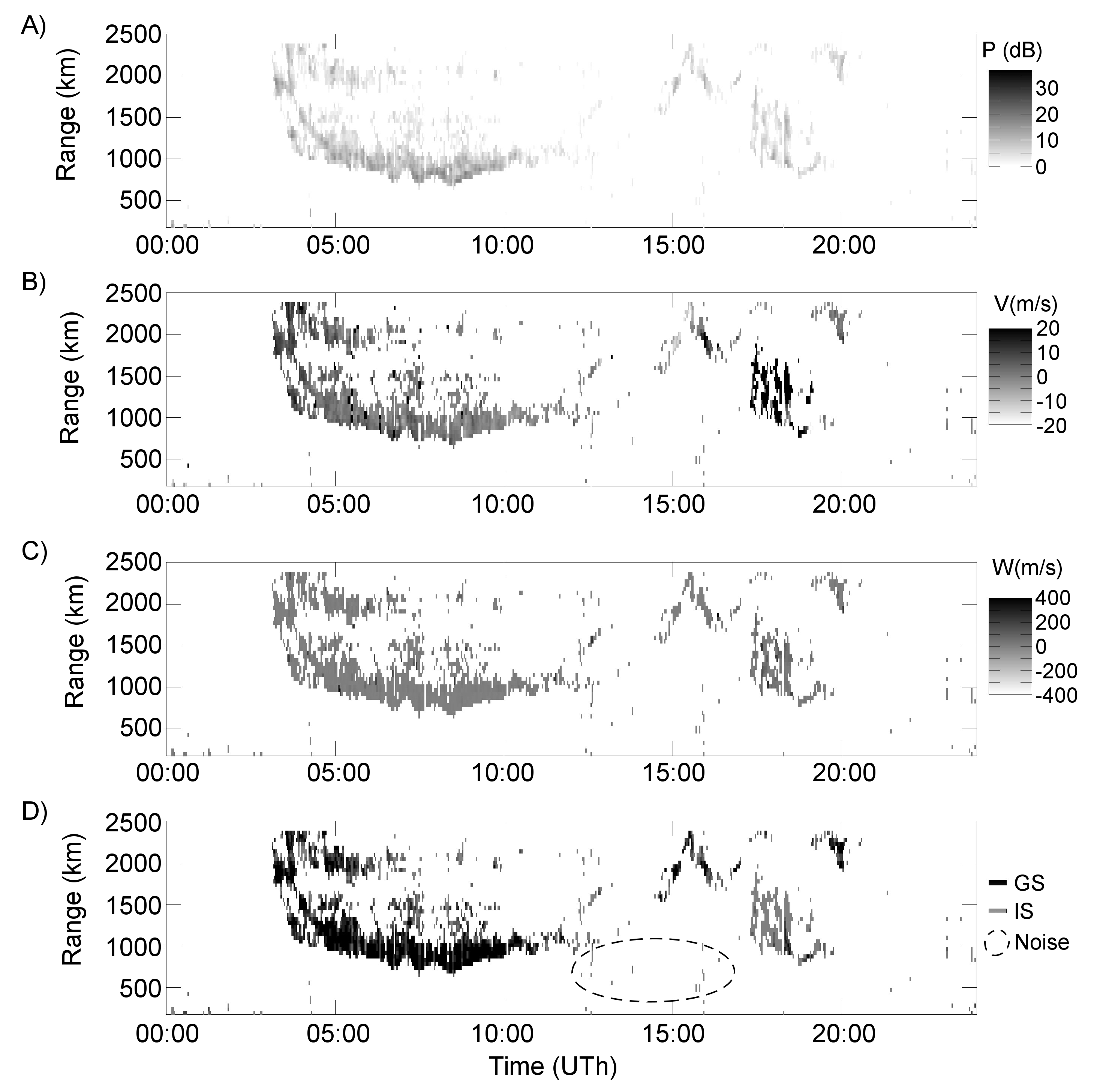
Figure 1: An example of scattered signals received at EKB ISTP SB RAS radar (at single beam). From the top to the bottom: A) is the power of the scattered signal; B) is the Doppler velocity in the range -40 - 40 m/s; C) is the spectral width in equivalent velocity units; D) signal types detected by standard SuperDARN program FITACF (groundscatter flag) and noise

The standard mode of the radar operation is the measurement of the average correlation function of the signal and using it to estimate the scattering irregularities parameters. The basic technique of parameter estimation is the standard FITACF program, developed and improved by the SuperDARN community [Ribeiro et al.(2013b)]. The main irregularities parameters produced by the FITACF program are the scattered signal power, Doppler shift and spectral width, estimated in two models of the correlation function - exponential and Gaussian [Hanuise et al.(1993)]. Fig.1shows an example of the data obtained at EKB ISTP SB RAS radar (at one of its beams). In Fig.1 shown the areas corresponding to the basic kinds of scattered signals analysed by the radar: the signal scattered from the earth’s surface (groundscatter,GS), the signal scattered from ionospheric irregularities (ionospheric scatter, IS), scattering from meteor trails (meteor echo) and noise. In Fig.1 one can see the well known basic characteristics of the received signals: low velocities and spectral widths of GS signals, high velocities and spectral widths of IS signals, and spatio-temporal fragmentation and short radar ranges of the meteor echo.

The standard approach to separating signals of different types is the separation based on the spectral parameters of the mean autocorrelation function - the spectral width and Doppler frequency shift. In this approach the GS signals are usually detected by small values of both parameters, not exceeding 30-40 m/s [Blanchard et al.(2009)], and the IS signals are detected by large values of these parameters. The problem of separating these two signal kinds is extremely important in the case when the ionospheric irregularities have a narrow spectrum and a small Doppler shift, which is sometimes observed when the drift of the irregularities is perpendicular to the radar line-of-sight. In this case, the described technique can lead to significant failures, and one should use more complex techniques, for example, cluster analysis [Ribeiro et al.(2011)]. Often these techniques are poorly justified from the physical point of view. The main task of the paper is to build a physically clear model of the scattered signal for both IS and GS, that takes into account their phase structure and allowing their separation.

Currently, at SuperDARN radars (similar to EKB ISTP SB RAS radar), there is a great emphasis on measurements of the full waveform of the scattered signal. The use of a full waveform is useful in the studies of meteor echo [Yukimatu and Tsutsumi(2002)], the digital formation of antenna pattern [Parris et al.(2008)] and in many other problems.

An essential problem useful for producing techniques for processing scattered signals the models of the signals. A relatively standard approach to simulating a scattered signal is the model of a large number of random scatterers [Rytov et al.(1988), Ishimaru(1999)]. As it was shown earlier, the model corresponds well to the experimental data [Farley(1969), Moorcroft(1987), Andre et al.(1999), Moorcroft(2004)] and can be used to producing realistic simulators of the received data [Ribeiro et al.(2013a)], and to develop signal processing techniques for signals accumulated over small number of sounding runs (realizations) [Reimer et al.(2016)].

Earlier we analysed individual realizations of the signal scattered by field-aligned ionospheric irregularities based on Irkutsk incoherent scatter radar data. We demonstrated [Grkovich and Berngardt(2011)] that the signal scattered by such irregularities in the VHF frequency band can be represented as a superposition of a small number of elementary responses. The shape of the responses repeats, in the first approximation, the shape of the sounding signal, but has random Doppler shift and random initial phase. The Doppler shift range is determined by the average spectrum of the scattered signal. The checking of the adequacy of the model for short radio waves requires a high sampling rate, of the order of a few points per duration of the sounding signal, and it is a critical requirement.

Currently, only a small number of SuperDARN radars have the capability of digitization of the signal with high sampling rate, for example [Parris et al.(2008)]. Initially, the EKB radar did not have this capability, digitizing a signal with low duty cycle (one point per sounding pulse duration). To investigate the fine structure of the scattered signals the radar was reprogrammed by us to work in the mode of increased sampling frequency. The maximal sampling frequency achieved by us in a regular mode is 5 points per pulse duration. In a special mode with non-standard sounding sequences, we have achieved the sampling frequency of 15 points per pulse duration ($T_{d}=20mks$ and $T_{p}=300mks$, respectively). In terms of range resolution these values correspond to $L_{d}=3km$ and $L_{p}=45km$.This sampling frequency does not allow us to measure the correlation function of the signal, so it is not used in regular measurements. The use of such a high sampling frequency makes it possible to study in detail the phase structure of scattered signals and makes it possible to verify the models of the scattered signal in regular mode (with 5 points per pulse duration) and special mode (with 15 points per pulse duration).

As a criterion that determines the quality of the scattered signal model, we have chosen its adequacy for the solution of an actual and widely studied problem - the problem of separating groundscatter signals (GS) and ionospheric scatter (IS).

Making special experiments significantly increases the amount of received information, so we conducted several experiments with a temporal resolution 15 points per pulse in various geophysical conditions during October 22, November 2-4, December 8-11, 2016, January 5 and April 26-27, 2017 . The regular observations with a temporal resolution 5 points per pulse are conducted from February 2017 till now. Further in the paper the data obtained during these experiments are used.

The study was conducted as follows. From the obtained set of experimental data, we manually selected two test data sets (for GS and IS signals) to in each set there was only one intense response over range - either first-hop groundscatter (GS) or ionospheric scatter (IS) , and we have no significant doubt about the nature of scattering in each particular. For GS signal we selected the region with a specific horseshoe-shaped spatio-temporal dependence of range vs. time; for the IS, mainly we used mostly evening and night responses and some observations of daytime ionospheric scatter clearly separated from the groundscatter.

The search for the region of intense scattering was carried out in the range of distances of 180-2000 km. After it is found, a range of distances (range window) was investigated with a length $R_{w}=1000km$ (which corresponds to $T_{w}=6660\mu s$) centred at the position of the detected intensity maximum.

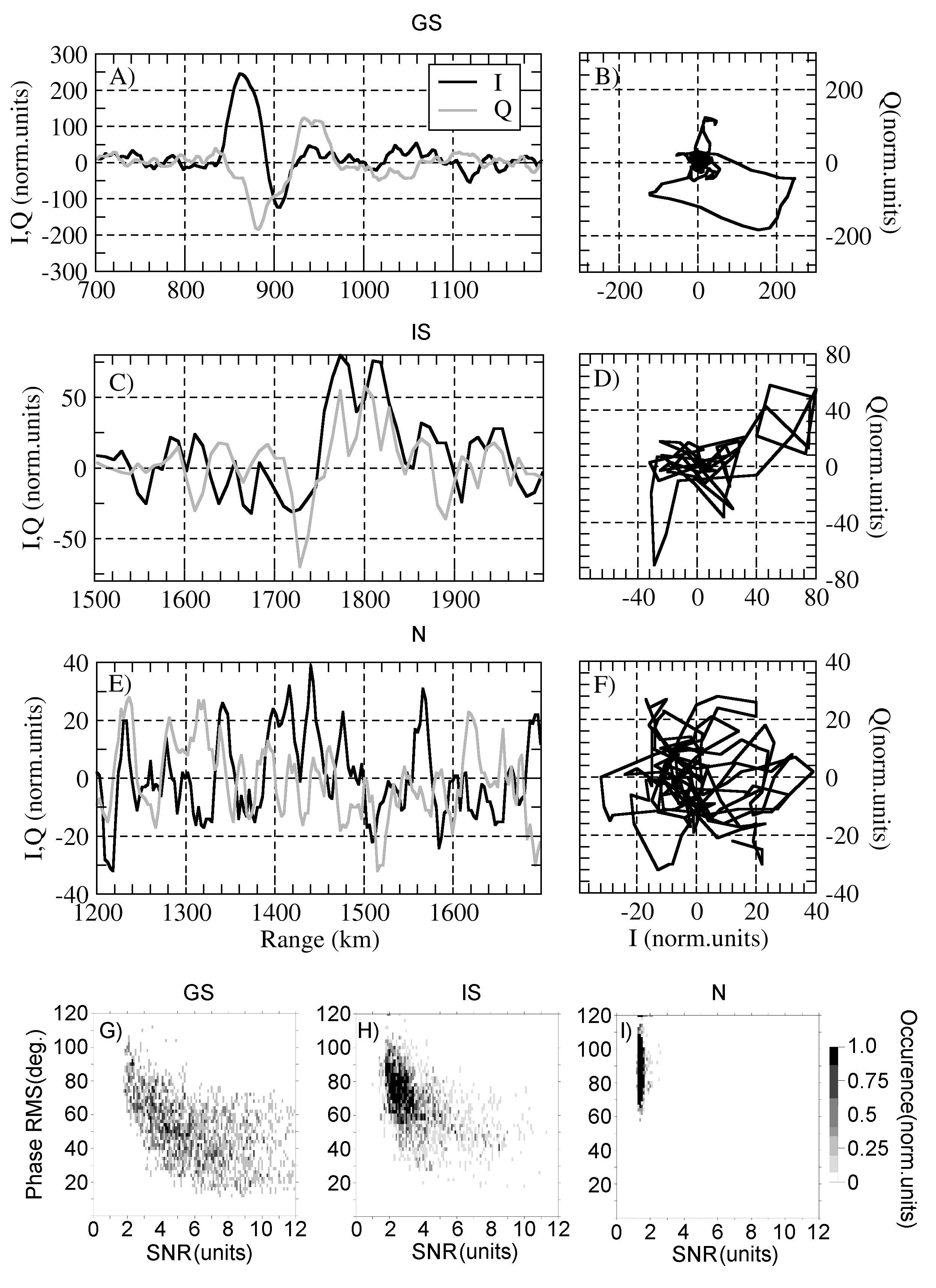
Figure 2: A-F) example of realizations of the received signal (quadrature components and phase of the signal) with a high sampling frequency in the cases of the groundscatter (A-B), the ionospheric scatter (C-D) and the noise (E-F). G-I) - Distributions of detected signals as a function of signal-to-noise ratio and the phase RMS (2) for different types of scattered signals: for groundbackscatter (G), for ionospheric scatter(H), and for noise(I).

Fig.2A-F shows examples of the received signal realizations (their amplitude and phase structure) in the cases of the groundscatter (Fig.2A-B), the ionospheric scatter (Fig.2C-D) and the noise (Fig.2E-F). The ionospheric scatter and groundscatter is chosen with a large signal-to-noise ratio, so that it is possible to confidently illustrate their amplitude-phase structure. It can be seen from the Fig.2A-F that both types of scattered signals (GS and IS) have a certain phase structure, which allows to considered them as non-random functions, in contrast to noise (N) with nearly no phase structure. To validate this assumption, we carried out a detailed analysis of the scattered signals on a large amount of data.

3 Coherent signal shapes

Due to presence of a specific phase-amplitude structure in the received GS and IS signals, it is of interest to parametrize this structure, create a semi-empirical model for it, and to determine the parameters of this model.

The GS signal has been studied for a long time in various experiments. It is known that this signal is formed by a strong refraction of the radiowaves in the ionosphere, leading to the focusing of radiowave at the boundary of the dead (skip) zone (a zone at which the receiving of radiowaves at a given frequency is impossible) [Budden(1985)]. Scattering of this high-amplitude signal by the ground surface irregularities causes a strong received signal at a range corresponding to the range to the boundary of the dead zone. The irregularities of the Earth’s surface with scales of the order of the wavelength (tens of meters) are nearly quasistationary (with the exception of the sea surface). The background ionosphere at the scales of the Fresnel zone radius (of the order several kilometres) is responsible for focusing the radio signal and also varies relatively slowly. Therefore, the GS signal is nearly stationary one in the first approximation, the range to it is also nearly constant. Thus, it can be qualitatively described from realization to realization, as a signal with an static phase-amplitude shape at a constant range, only its initial phase can vary from realization to realization. There are analytical expressions describing the dependence of the power of this signal on the range [Tinin(1983)]. They predict an asymmetry of its shape relative to the position of its maximal energy, and this corresponds well with experimental observations at radars [Bliokh et al.(1988)].

The amplitude-phase structure of the ionospheric scatter signal without averaging is practically not investigated, and the conventional models are practically absent. Only statistical models exist. In the framework of the ionospheric scatter model considered for analogous irregularities in the VHF band [Grkovich and Berngardt(2011)], it was shown that the scattered signal is in most cases can be interpreted as a single response of the shape that repeats the sounding signal and differs from realization to realization only by the initial phase and Doppler shift. By analogy, let’s consider the same model in HF. In addition, let’s assume that the position of the scattering region is stationary and Doppler shift is nealy zero. The assumption of nearly zero Doppler shift does not contradict the [Grkovich and Berngardt(2011)] model, since the sounding pulse is short and phase changes within single pulse duration are very small too (the possible irregularities Doppler drift velocities are within 1 km/s, for sounding frequency 10-11MHz and for sounding pulse duration $300\mu s$ this lead to a phase variations of not more than 8 degrees).

The assumption we made about the stationarity of the scatterer position is more strict. From qualitative considerations, it can be justified as follows: within the radar equation in presence of refraction [Berngardt et al.(2016)], the locations of effective scattering that are equivalent to the scattering at a point object are the locations with a given level of refraction in which at the same time an aspect sensitivity conditions are satisfied. Thus, their positions in the first approximation are determined by relatively large-scale structure of the ionosphere and the magnetosphere and have a relatively slow dynamics. Therefore, we can assume that this assumption is also fulfilled, later we will check this from experimental data. Thus, even in the case of different Doppler drifts (for the characteristic velocities <1 km/s observed in the experiment), within the framework of the [Grkovich and Berngardt(2011)] model the scattered signal can be interpreted as a number of pulses with similar amplitude and phase structure located at approximately the same radar range from realization to realization.

Thus, the unified signal model that describes in the first approximation both GS and IS signals is a signal that has unknown amplitude-phase shape at constant range that does not change from realization to realization and that has an initial phase varying from realization to realization. To determine the unknown shape of such an elementary response for both kinds of signals (GS and IS), we used the coherent accumulation technique. This technique is based on finding in each realization the unknown initial phase and on coherent accumulation of the signals over the realizations with taking into account these initial phases.

The first step of the technique is to determine the position (radar range or radar delay $\tau_{o}$) of the most powerful scattering, carried out by searching for the maximal signal-to-noise ratio averaged over a given number of realizations of the scattered signal (in our case, 20 successive sounding sequences). In this case, the average signal level is determined as the mean square of the signal amplitude modulus over a time window equal to the duration of the elementary sounding pulse ($300mks$). The average noise level is calculated as the average signal level over the entire radar range (the pulse duration refers to the entire radar range as $1/40$). The signal-to-noise ratio calculated in this approach is insignificantly different from real signal-to-noise ratio at its small values. At high signal-to-noise rations it constraints the signal-to-noise ratio at the level of about 40, which improves the stability of the technique to random noise-like bursts.

At the second stage, the parameters $(k,\psi_{0},\psi_{1},....\psi_{n})$ of model phase $\phi_{i}^{M}\left(t,k,\psi_{i}\right)$ are determined for the phase dependence $\phi_{i}(t)$ for each of the signals. The model $\phi_{i}^{M}\left(t,k,\psi_{i}\right)$ is:

$$\phi_{i}^{M}\left(t,k,\psi_{i}\right)=k\cdot(t-\tau_{o})+\psi_{i}$$ (1)

The calculation of the parameters is made over the region limited by the duration of the sounding pulse with the centre at the delay $\tau_{o}$.

As already mentioned, even the strong Doppler shifts observed in the ionosphere, at the durations of the sounding pulse order lead only to a slight phase changes. Therefore, the use of the linear model (1) for the phase of elementary scattering response is sufficient and justified. The parameter $k$ is the phase distortion factor or Doppler shift and is assumed to be the same for all implementations. The parameter $\psi_{i}$ is the initial phase of the scattered signal and varies from realization to realization.

All the $N_{r}+1$ parameters of the model (1) are determined based on the minimization condition for the root mean square (RMS) deviation of the phase $\Omega$:

$$\Omega=\sqrt{\frac{1}{N_{r}T_{p}}\sum_{i=1}^{N_{r}}\int_{\tau_{0}-\frac{T_{p}}{2}}^{\tau_{0}+\frac{T_{p}}{2}}\left(\phi_{i}(t)-\phi_{i}^{M}\left(t,k,\psi_{i}\right)\right)^{2}dt}=min$$ (2)

Due to the fact that the model phase (1) is linear over all the parameters, the problem (2) reduces to a system of linear equations and can be solved analytically.

The root-mean-square deviation, at which the minimum of the functional (2) is reached, determines the root-mean-square deviation of the phase from the linear law, and can be used to verify the adequacy of the model (1). Fig.2G-I shows the distributions of detected signals with maximal amplitudes, as a function of signal-to-noise ratio and the phase RMS (2) for different types of scattered signals: for groundbackscatter, for ionospheric scatter, and for noise. It can be seen from the Fig.2G-I that the noise is characterized by signal-to-noise ratios about 1.5 and by phase RMS over $90^{o}$, which indicates its quasi-random nature and approximately constant amplitude over the range. Between the distributions of ionospheric scatter and ground backscatter there are no specific differences except smaller signal-to-noise ratios of ionospheric scatter.

At the third stage, all the realizations in the studied group are rotated by their initial phases $\psi_{i}$ computed at second stage and added together, so the signal accumulation in the region of the maximal signal-to-noise ratio is made with nearly the same phase. The result of accumulation is normalized to the number of realizations in the group:

$$U(t)=\frac{1}{N_{r}}\sum_{i=1}^{N_{r}}u_{i}(t)e^{-i\psi_{i}}$$ (3)

The average waveform thus obtained can be used for the subsequent analysis of the mean structure of the scattered signal.

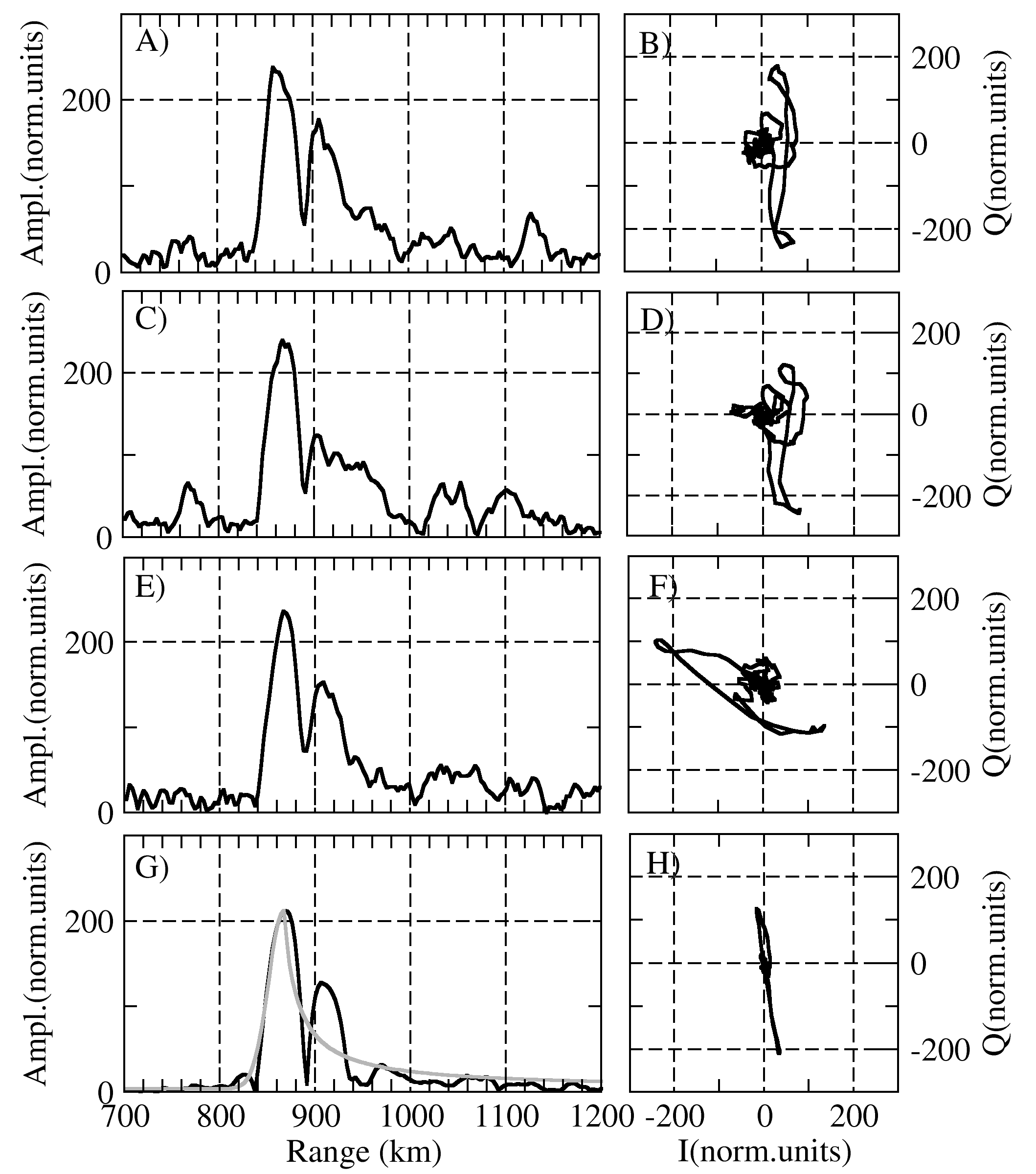
Figure 3: Ground backscatter signals - amplitude (A,C,E,G) and phase diagrams (B,D,F,H). A-F) 3 consequent realizations in the group G-H) Coherently accumulated signal over 30 sounding pulses (~300msec). The grey line shows the approximation of the accumulated signal by the model (3).

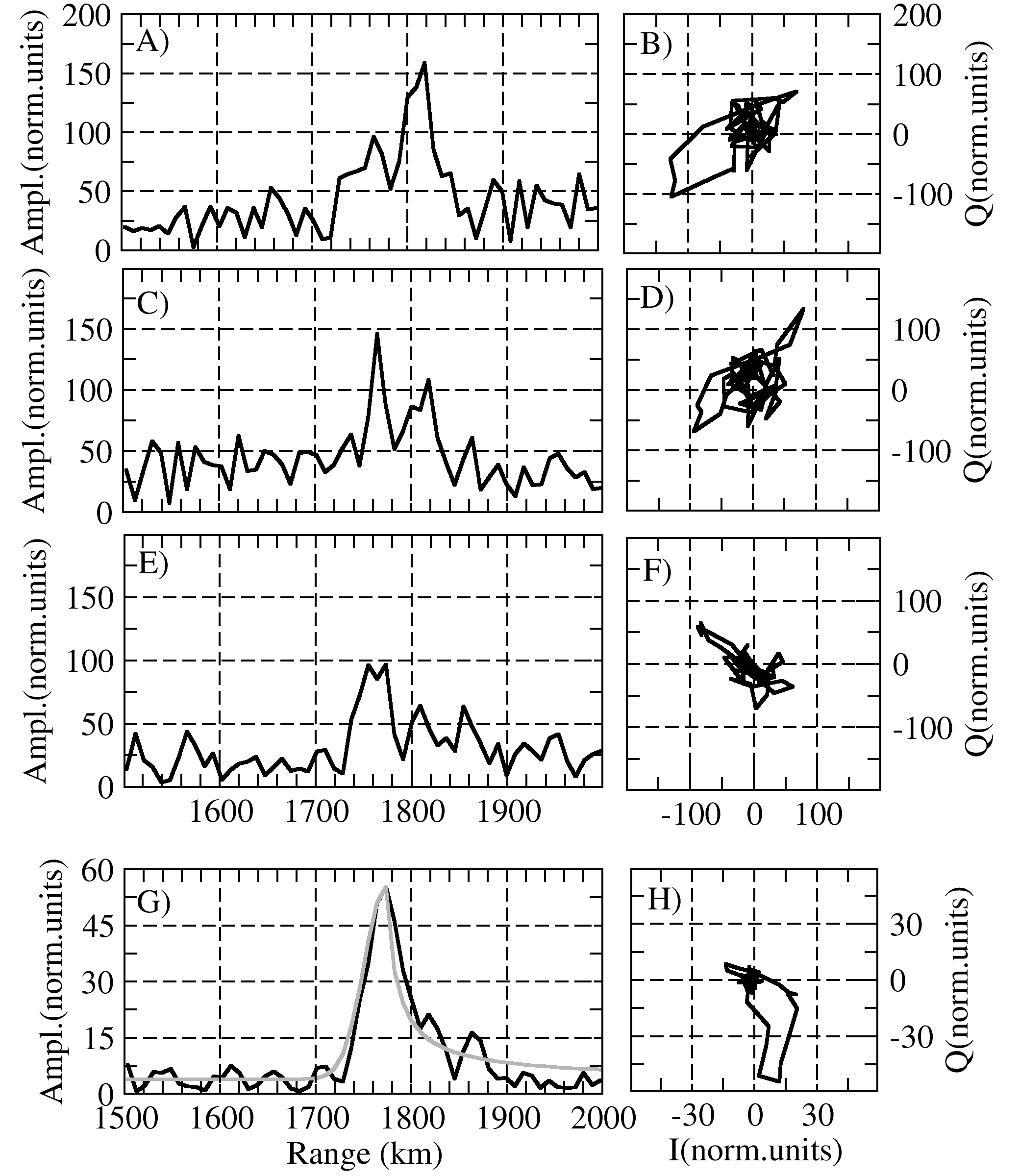
Figure 4: Ionospheric scatter signals - amplitude (A,C,E,G) and phase diagrams (B,D,F,H). A-F) 3 consequent realizations in the group G-H) Coherently accumulated signal over 30 sounding pulses (~300 msec). The grey line shows the approximation of the accumulated signal by the model (3).

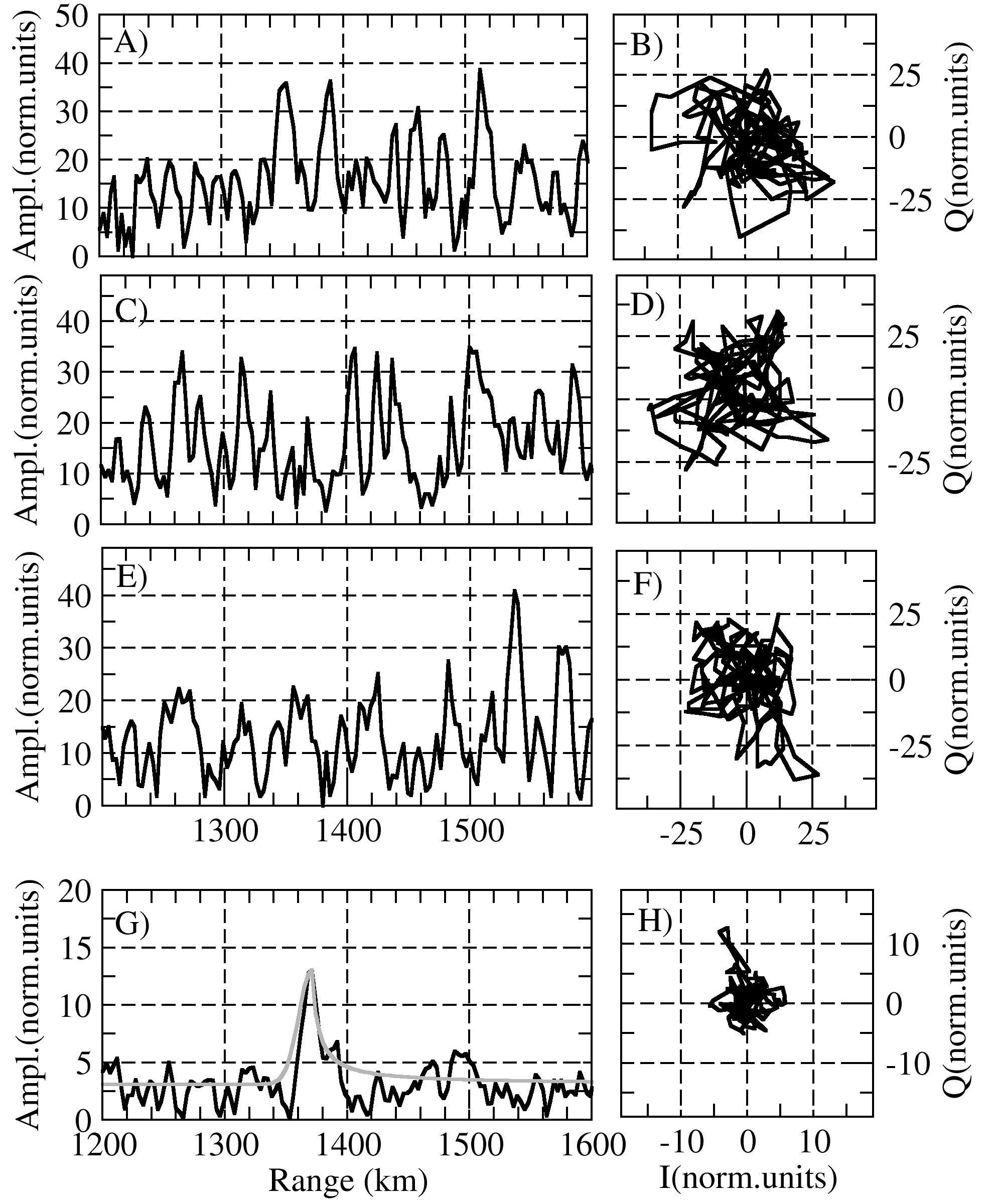
Figure 5: Noise signals - amplitude (A,C,E,G) and phase diagrams (B,D,F,H). A-F) 3 consequent realizations in the group G-H) Coherently accumulated signal over 30 sounding pulses (~300 msec). The grey line shows the approximation of the accumulated signal by the model (3).

In Fig.3, Fig.4 and Fig.5 shown an examples of ground backscatter signals, ionospheric scatter signals and noise signals, as well as the mean shape of these signals. It can be seen from the figures that the mean shape of the ground backscatter signal, in contrast to the ionospheric scatter signal and noise, is essentially asymmetric and has a more prolonged right edge.

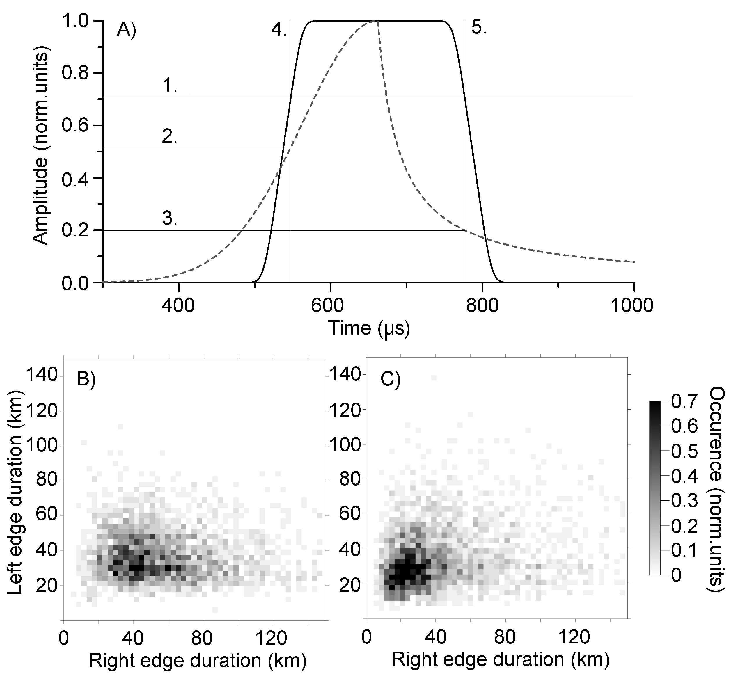
Figure 6: A) Normalization of the threshold levels of the approximating functions based on the sounding pulse. marks 1-5 are the following: 1 is level of half power (0.7 in amplitude) of the sounding signal. 2 is the threshold level for approximating the left edge. 3 is the threshold level for approximating the rigth edge; 4 is the moment corresponding to half power on the left edge of the sounding signal; 5 is the moment corresponding to half the power on the right edge of the sounding signal. B-C) are the distributions of edge durations of the received signals B) is the distribution for ground backscatter; C) is the distribution for ionospheric scatter.

To check the regularity of the observed feature, we made an algorithm to determine of the duration of the right and left edges of the accumulated signal and applied it to all the investigated observations. Obviously, the first step to estimating the edge duration is to create an unified model that can approximate both the GS signal and the IS signal. We used the following asymmetric model (illustrated at Fig.6A):

$$a(t,\{A,B,C\})=N+\left\{\begin{array}[]{l}Ae^{-\left(\frac{{}^{t-\tau_{0}}}{C}\right)^{2}};t<\tau_{0}\\ \frac{A}{1+(t-\tau_{0})/B};t>\tau_{0}\end{array}\right.$$ (4)

where $\tau_{0}$, $A$ are the radar delay to the maximal amplitude of the scattered signal and the maximal amplitude of the accumulated signal correspondingly; $N$ is the noise level, defined as the sum of the constant noise level and its RMS (determined at large distances, where the groundscatter and ionospheric scatter signals are absent); $B$ and $C$ are the parameters to be estimated, that characterize the duration of the left and right edges, respectively. The choice of this model can be qualitatively justified by the form of the asymptotic solution for the GS power, characterized by a sharp left edge, and by the smooth right edge [Tinin(1983)]. The comb structure of the accumulated signal, as well as its phase structure has not been investigated in the paper. In order to speed up the calculations, the search for $B$ and $C$ values was made based on integral approach: the integral on the left and right of $\tau_{0}$ of the experimental signal shape should be equal to the corresponding integral of the model function:

$$\left\{\begin{array}[]{l}\int_{\tau_{0}}^{\infty}(a(t,\{A,B,C\})-N)dt=\int_{\tau_{0}}^{\infty}(U(t)-N)dt\\ \int_{0}^{\tau_{0}}(a(t,\{A,B,C\})-N)dt=\int_{0}^{\tau_{0}}(U(t)-N)dt\end{array}\right.$$ (5)

After determining the parameters of the model $B,C$ it is necessary to calculate from them the durations of left and right edges correspondingly. The calculation should be made by the special way to the model time-symmetric sounding signal has the same right and left edges the sum of which is equal to actual sounding signal duration.

To migrate from the parameters of model $B$ and $C$ to the edge durations $T_{R},T_{L}$, we determined at which threshold levels $\varepsilon_{L,R}$ the two functions: $e^{-\left(\frac{{}^{t-\tau_{0}}}{C}\right)^{2}}$ and $\frac{1}{1+(t-\tau_{0})/B}$ intersect with the model shape of a Gaussian signal signal with standard $300mks$ duration. The values of these threshold levels are found to be $\varepsilon_{L}=0.5$ for the left edge and $\varepsilon_{R}=0.2$ for the right edge. Thus, the duration of the edges $T_{L},T_{R}$ are defined by us as the distance from $\tau_{0}$ to the points at which the right or left edge of the model function reach the right or left threshold level:

$$\left\{\begin{array}[]{l}a(t-T_{L},\{A,B,C\})=\varepsilon_{L}A+N\\ a(t+T_{R},\{A,B,C\})=\varepsilon_{R}A+N\end{array}\right.$$ (6)

The edge durations $T_{L},T_{R}$ determined in this approach have a clear physical sense - when the model (4) is fitted into a real sounding signal $a_{0}(t)$ of $300\mu s$ duration, the calculated edge durations $T_{L},T_{R}$ will be equal to $150mks$ each (half of the sounding pulse duration). An explanation of this method for estimating the edge duration is illustrated in Fig.6. Therefore, the obtained values of $T_{L},T_{R}$ can be used to quantitatively compare the durations of the right and left edges with the duration of the sounding signal, and thus allow us to estimate duration of the scattered signal edges directly in kilometres or microseconds.

By using the technique described above, we calculated the statistical distributions of the durations of the left and right edges for IS and GS signals, based on the the available experimental data (Fig.6B-C). From the figure one can see that the characteristics of the scattered signals of different kinds are significantly different: the accumulated ground backscatter signal (Fig.6B) is more asymmetric and has smoother right edge in comparison with the right edge of the ionospheric scatter signal (Fig.6C). At the same time, the accumulated ionospheric scatter signal has relatively symmetrical edges. This does not contradict the previously developed models for GS[Tinin(1983)] and IS [Grkovich and Berngardt(2011)] signals, and validates the use of these models in the problem under consideration.

4 Coherent signal lifetimes

Traditionally, the HF signal scattered from ionospheric irregularities is interpreted as a superposition of scattering from the large number of elementary scatterers [Farley(1969), Moorcroft(1987), Andre et al.(1999), Moorcroft(2004)]. In the previous section, we showed that in the case of scattering by field-aligned irregularities it can be interpreted as a result of scattering by a small number of elementary scatterers spaced in range, which is closely related to the model we proposed earlier in VHF [Grkovich and Berngardt(2011)].

Let’s estimate the characteristic lifetimes of such elementary scatterers from the scattered signal. To do this let’s find the dependence of the normalized cross-correlation coefficient between two different realizations, as a function of the delay between them. Following to the approach described before the calculation of the correlation coefficient is made over a region of maximal signal-to-noise ratio, centred at delay $\tau_{0}$. The duration of the region is determined from the statistics of coherently accumulated signals - as the maximal expected durations of the right and left edges $T_{R,0},T_{L,0}$.

$$R(i)=max_{n}\left\{R_{n,n+i}(t)=\frac{\int_{\tau_{0}-T_{L,0}}^{\tau_{0}+T_{R,0}}u_{n}(\tau)u_{n+i}^{*}(\tau+t)d\tau}{\sqrt{\int_{\tau_{0}-T_{L,0}}^{\tau_{0}+T_{R,0}}|u_{n}(\tau)|^{2}d\tau\int_{\tau_{0}-T_{L,0}}^{\tau_{0}+T_{R,0}}|u_{n+i}(\tau)|^{2}d\tau}}\right\}$$ (7)

where $u_{n}^{*}$ is the complex conjugate value of the signal $u_{n}$ received in n-th sounding run.

As one can see in Fig.3,6B, the duration of ground backscatter signal in a single realization (before its coherent accumulation) can reach up to 200-300 km. At the same time, the duration of the left edge for both kinds of signals usually does not exceed 60 km ($400\mu s$, see Fig. 6B-C).

Therefore, we chose the following values for the duration of the right and left edges used for calculation of correlation coefficient (7) $T_{R,0}=400mks$, $T_{L,0}=1600mks$.

For a detailed analysis of the irregularities lifetime we developed an algorithm for calculating the correlation coefficient at arbitrary moments, both comparable with and exceeding the duration of the sounding sequence (70 ms). The basis of the algorithm is the calculation of the correlation coefficient at delays (lags) corresponding to the combination lags between the sounding pulses. The main property of the sounding sequences, based on the properties of Golomb rulers, is that the combination lags between different sounding pulses are always different and practically uniformly cover the region of lags within the duration of the sounding sequence. The correlation coefficient for signals at such combinational delays makes it possible to determine the dependence of the correlation coefficient at small lags that are shorter than the sequence length.

Analysis of the correlation coefficient at lags exceeding the duration of the sounding sequence is traditionally not carried out at SuperDARN radars and at EKB radar. Most often this is associated with the complexity of the end-to-end synchronization of all sounding sequences. In the approach we proposed, this is possible. To evaluate the correlation coefficient at large lags exceeding the duration of the sounding sequence we calculated it at lags equal to the delay between the response from the first pulse of the first sounding sequence and the pulses of all subsequent sounding sequences. This approach allows us to obtain a detailed dependence of the correlation coefficient at nearly arbitrary lags.

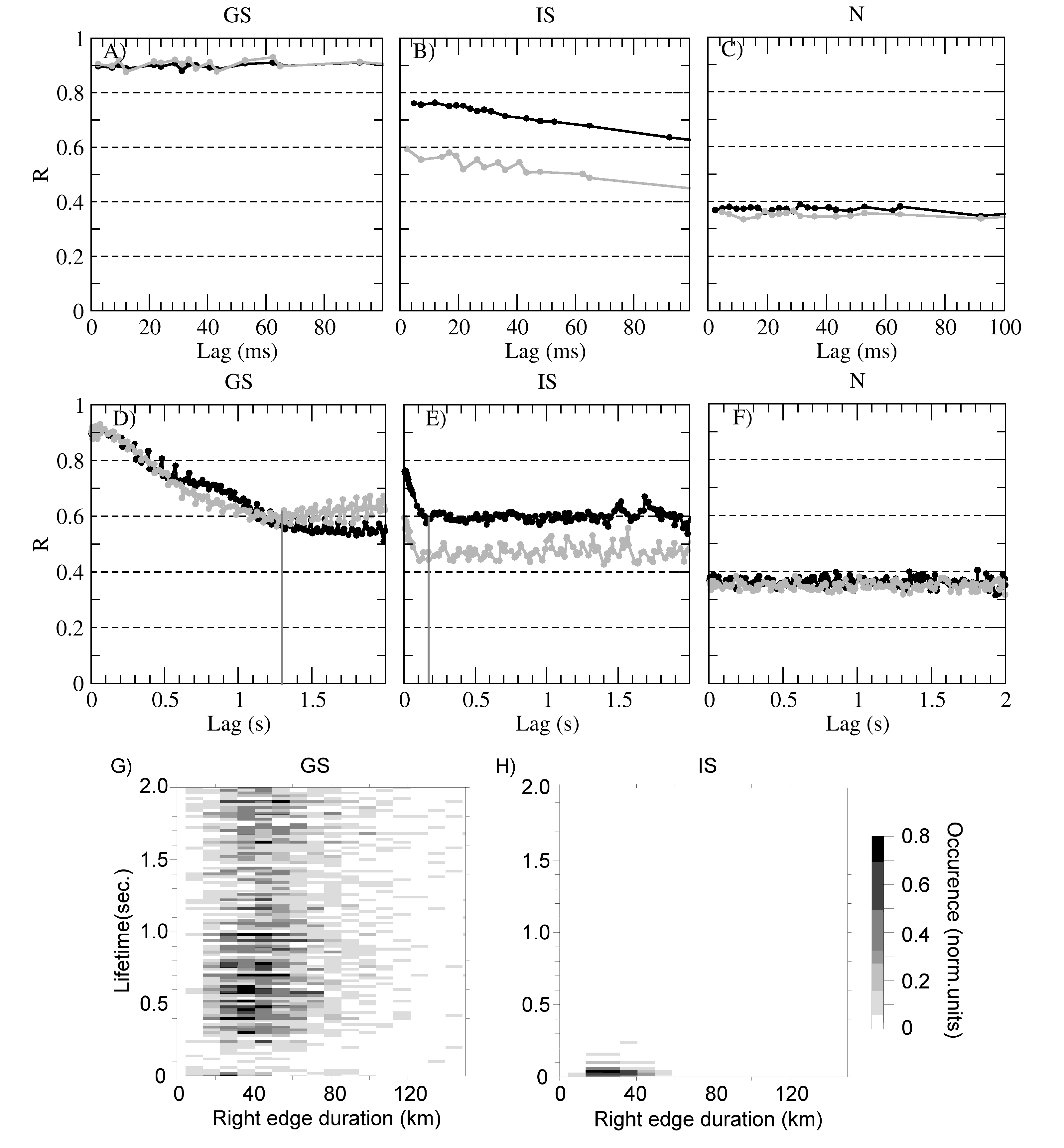
Figure 7: A-F) - correlation coefficient for different signal types. A-C) are is correlation coefficient at small lags comparable with sounding sequence duration for groundscatter(A), for ionospheric scatter(B) and for noise (C); D-F) is correlation coefficient at large lags comparable with averaging interval in regular sounding mode, for groundscatter (D), for ionospheric scatter (E) and for noise (F). Grey veritcla line at D-E corresponds to coherent signal lifetime. G-H) - distributions of signals over the scatterer lifetime (in seconds) and the right edge duration (in km.): G) is the distribution for ground backscatter; H) is the distribution for ionospheric scatter.

Examples of the algorithm functionality for different kinds of scattered signals are shown in Fig.7. It can be seen from the fig.7A-C the groundscatter and ionospheric scatter signals differ significantly from the noise - they have higher correlation coefficient at small lags. The correlation coefficient for IS signals increases at small lags, and this allows to interpret the IS signal as a result of scattering by scatterers with a relatively short lifetime (hundreds of milliseconds). This does not contradict the existing data on the lifetime of instabilities that form field-aligned irregularities [Villain et al.(1996)]. It should be noted that when the signal noise ratio decreases, this property still persists, although it becomes less pronounced, and the maximum correlation coefficient at small lags decreases.

Ground backscatter signals also tends to decrease the correlation coefficient with a lag, but the characteristic rate of the decrease is much lower. From Fig.7A-B one can see, that in some cases (black lines) it is difficult to differ groundscatter from ionospheric scatter using lifetime (small IS spectral widths case) at lags, provided by standard sounding sequences. At other cases (green lines in 7A-B) they can be differed (big IS spectral widths case).

Analysis of correlation at extra large lags, compared with whole averaging interval for regular sounding is shown in Fig.7D-F. It can be seen from Fig.7D-F that when analysing extra large lags, the average lifetime of GS signals (>1s) exceeds the lifetime of IS signals(<250ms).

This can be explained by the physics of their formation - GS signal is a signal scattered by nearly stationary ground surface inhomogeneities, and its nonstationarity is mainly related with the existence of medium- and large-scale ionospheric irregularities that affect the refraction of this signal and, accordingly, its decorrelation with time. On the other hand, it is known that the lifetime of individual small-scale inhomogeneities is small, and can be estimated from the spectral width of the IS signals (rarely exceeds $250ms$. Thus, the lifetime data obtained by us do not contradict the known characteristics of the scattered signals and the physics of their formation.

To automaticaly calculate the lifetime we use the following technique. In Fig.7D-E one can see that correlation coefficient falls with delay (’lag’) and reaches a certain stable (’noise’) level. Therefore we define the lifetime as delay at which the correlation coefficient is bigger than certain threshold level $R_{th}$. This level is calculated over large lags, as $R_{th}=<R>+\Delta R$. Here

$$\begin{array}[]{l}<R>=\frac{1}{T_{2}-T_{1}}\int_{T_{1}=2sec}^{T_{2}>T_{1}}R(t)dt\\ \Delta R=\sqrt{\frac{1}{T_{2}-T_{1}}\int_{T_{1}=2sec}^{T_{2}>T_{1}}(R(t)-<R>)^{2}dt}\end{array}$$ (8)

5 Separation of IS and GS signals

As was shown earlier in the paper, GS and IS signals have different characteristics of the mean shape of the scattered signal and different lifetime (correlation) of the elementary scatterer. This allows us to construct effective techniques for separating these signals by their amplitude-phase and correlation characteristics.

One of the standard approaches to signal separation is the method for testing statistical hypotheses [Lehmann and Romano(2005)]. This method reduces the problem of separating signals to the problem of determining the detection boundary shape in the multidimensional space of signal characteristics, on the one side of which the signal will be considered as GS signal, and on the other side of the boundary it will be considered as IS signal. There are several methods of making such a boundary shape, and they are based on minimizing the sum of the errors of the first and second kind (errors of incorrect acceptance and incorrect rejection of the hypothesis). We used the simplest Bayesian inference, under assumption of the equiprobability of IS and GS signals.

As it was shown earlier in the paper, the basic characteristic parameters that allow separation are the scatterer lifetime (correlation time) and the duration of the right edge of the coherently accumulated signal. Fig.7G,H shows the distributions of these GS and IS signal characteristics - the right edge duration (in km.) and the scatterer lifetime (in seconds). It can be seen from the figure that in these coordinates, the IS signals area corresponds to a small region concentrated near small lifetimes (y-axis) and edge durations(x-axis) oriented along the x-axis. The most part of the GS signals are outside this region. So the Bayesian approach should provide effective solution for separation.

To separate these kinds of signals, we used the distribution of their characteristics in a three-dimensional parameter space (the duration of the right edge, the duration of the left edge, and the scatterer lifetime). Earlier it was shown (fig.7G-H) that the IS signal distribution lies within a closed region in the parameter space bounded by a certain surface around the coordinates centre (small lifetimes, short right edges). The GS signal distribution in this parameter space lies outside this surface (large lifetimes, long right edges). In the first approximation, there is no significant correlation between the duration of the right edge and the scatterer lifetime (Fig.7G-H), as well as between the left and right edges of the coherently accumulated signal (Fig.6). Therefore, in the first approximation, we can use separation boundary as the surface of a certain ellipsoid with the axes along the coordinate axes:

$$\frac{x^{2}}{a^{2}}+\frac{y^{2}}{b^{2}}+\frac{z^{2}}{c^{2}}=1$$ (9)

The coordinates x, y and z in our case are the scatterer lifetime, the duration of the left edge and the duration of the right edge of the coherently accumulated signal, respectively. The elipsoid axis sizes - $a,b,c$ are to be determined.

To determine these parameters, three-dimensional discrete distributions $P_{IS}(x,y,z)$ and $P_{GS}(x,y,z)$ were constructed from two experimental data sets (for GS and for IS). The step of the discretization of distributions over the scatterer lifetime was 2.5 ms, and over the left and right edges - 3 km. The search for the optimal values of the parameters $a,b,c$ was made numerically, by a direct search over the grid by the parameter (in steps of 2.5 ms for $a$, and 3 km for $b$ and $c$). The condition for optimality of the parameter set was the Bayesian criterion in the form of minimization of the functional of the total error of the first and second kinds:

$$\Omega=\int_{r\left(\theta,\alpha\right)>\rho_{d}\left(\theta,\alpha\right)}P_{IS}(x,y,z)dxdydz+\int_{r\left(\theta,\alpha\right)<\rho_{d}\left(\theta,\alpha\right)}P_{GS}(x,y,z)dxdydz=min$$ (10)

Integration in the Cartesian coordinate system is made over the region outside the surface of the ellipsoid in the first term, and over the region inside this ellipsoid - in the second term. Physically, this condition corresponds to the fact that most of the values of the scattered signal characteristics for ionospheric scatter lie inside the surface of the desired ellipsoid, and most of the values of the scattering characteristics of ground backscatter are outside the surface of this ellipsoid.

The coordinates of the ellipsoid in the calculations are given in the polar coordinate system $\left(r,\theta,\alpha\right)$. This makes it convenient to determine the condition if test point lies inside or outside the surface of the ellipsoid. In this case, it reduces the separation problem to checking the conditions $r\left(\theta,\alpha\right)>\rho_{d}\left(\theta,\alpha\right)$ and $r\left(\theta,\alpha\right)<\rho_{d}\left(\theta,\alpha\right)$, where $\rho_{d}\left(\theta,\alpha\right)$ is the equation of the ellipsoid surface in polar coordinates.

Based on the learn data set with more than 13 thousand realizations and optimum condition (10) we calculated the following separation boundary (9) parameters: a = 285 ms, b = 120 km, c = 429 km. We use about 19 thousand realizations to test the technique (13 thousand from learn data set and 6 thousand of other realizations) to verify the technique. The results are shown in Fig.8. As shown our analysis, the accuracy of groundscatter detection is about 95.1%. Accuracy of ionospheric scatter is about 88.6%. The total detection error is about 16%.

To illustrate the technique in Fig.8 we shown an example of detection of the type of signals for GS and IS signals based on the test data set described above. As one can see in Fig.8 in most cases the algorithm works correctly and the correctness of the response does not depend on the signal-to-noise ratio, which is an indirect sign of the validity of the developed model and the separation technique.

6 Conclusion

The analysis is made of the fine structure of decameter signals scattered by irregularities of the earth’s surface and field-aligned ionospheric irregularities. To carry out such an analysis with a high sampling frequency, the software of the EKB ISTP SB RAS radar was substantially modernized. A large number of experimental data with an increased sampling frequency has been obtained. As a result of the experimental data analysis it is shown that signals scattered by both mechanisms have a specific phase structure and a nonzero lifetime. This allows us to interpret them as signals scattered by a small number of localized irregularities with a finite lifetime. A method was implemented for detecting the shape of the elementary response. Empirical model is developed that allows to describe both types of signals and to determine their characteristics - the lifetime, the duration of the right and left edges. Statistical features of both types of scattered signals are estimated and presented. Differences in the shape of signals scattered from the earth’s surface and from the ionosphere are detected: the different durations of the right front of the signal and different lifetimes. Based on the analysis of the full waveform and the Bayesian inference approach, a method for the optimal separation of ground scatter and ionospheric scatter signals was constructed. The technique works without statistical averaging and without using traditional SuperDARN methods for estimating scattered signal parameters (FITACF). The effectiveness of the method is estimated based on EKB radar data, it shows total detection error about 16%.

7 Acknowledgements

The work was supported by the RFBR grant # 16-05-01006a. The functioning of the EKB ISTP SB RAS is supported by the FSR program II.12.2.3. The data of EKB radar is a property of ISTP SB RAS, contact berng@iszf.irk.ru

8 References

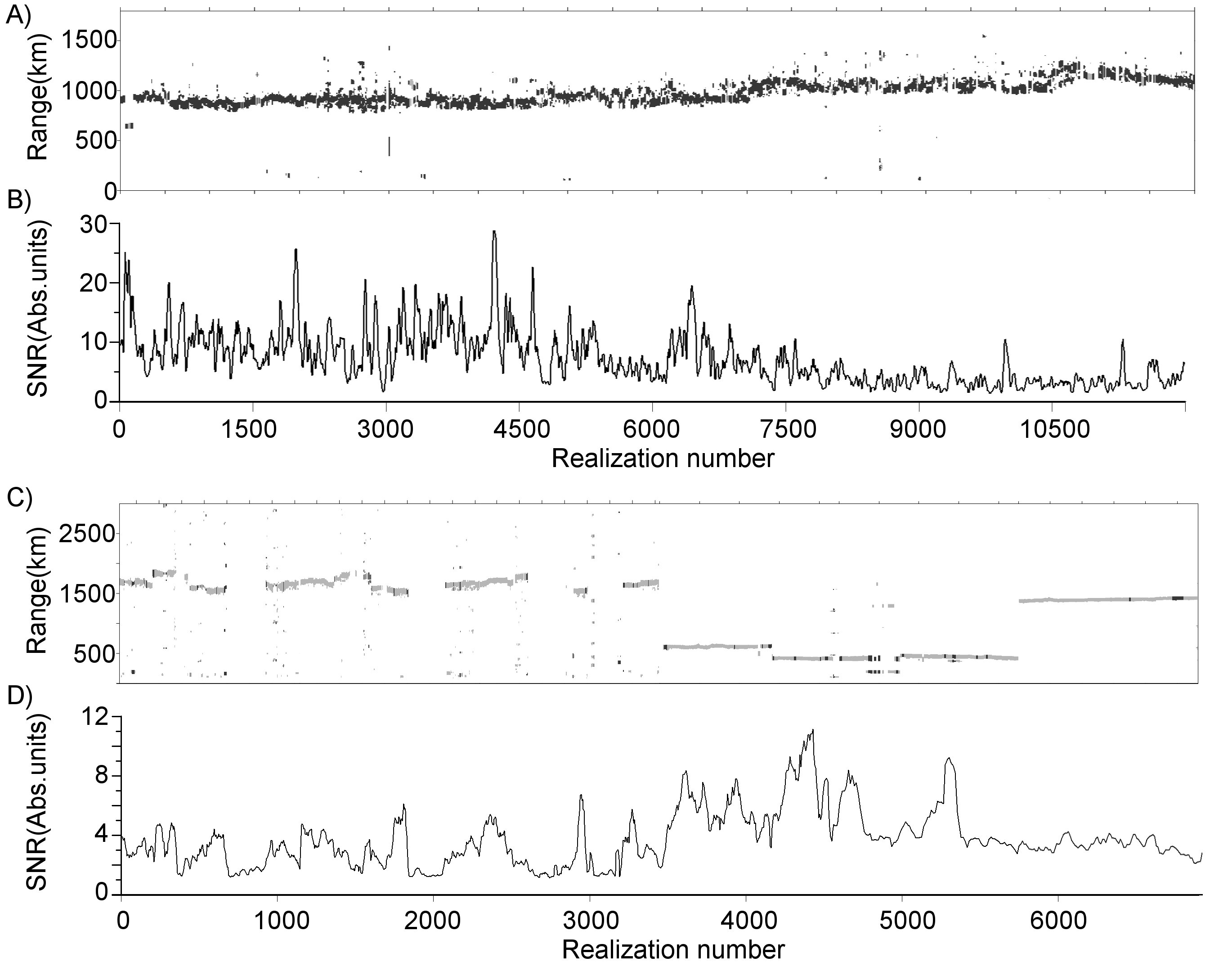
Figure 8: The results of detecting signal type by the new detection algorithm. Black color at (A,C) marks the signals, identified as groundscatter, grey color at (A,C) marks the signals identified as ionospheric scatter. A) - results of processing GS data; B) - peak signal-to-noise ratio of GS data; C) - results of processing IS data; D) is the peak signal-to-noise ratio of IS data.

References

- [Andre et al.(1999)] Andre D., Pinnock M., Rodger A.S.. On the SuperDARN autocorrelation function observed in the ionospheric cusp. Geophys Res Lett 1999;V.26(N.22):pp.3353–3356. DOI:10.1029/1999gl003658.
- [Barthes et al.(1998)] Barthes L., Andre D., Cerisier J.C., Villain J.P.. Separation of multiple echoes using a high-resolution spectral analysis for SuperDARN HF radars. Radio Sci 1998;V.33(N.4):pp.1005–1017. DOI:10.1029/98rs00714.
- [Berngardt et al.(2016)] Berngardt O., Kutelev K., Potekhin A.. SuperDARN scalar radar equations. Radio Science 2016;V.51(N.10):pp.1703 – 1724. DOI:10.1002/2016rs006081.
- [Berngardt et al.(2015a)] Berngardt O., Zolotukhina N., Oinats A.. Observations of field-aligned ionospheric irregularities during quiet and disturbed conditions with EKB radar: First results. Earth, Planets and Space 2015a;V.67:pp.143. DOI:10.1186/s40623-015-0302-3.
- [Berngardt et al.(2015b)] Berngardt O.I., Voronov A.L., Grkovich K.V.. Optimal signals of Golomb ruler class for spectral measurements at EKB SuperDARN radar: Theory and experiment. Radio Science 2015b;V.50(N.6):pp.486–500. DOI:10.1002/2014RS005589.
- [Blanchard et al.(2009)] Blanchard G.T., Sundeen S., Baker K.B.. Probabilistic identification of high-frequency radar backscatter from the ground and ionosphere based on spectral characteristics. Radio Science 2009;V.44(N.5):pp.RS5012. DOI:10.1029/2009rs004141.
- [Bliokh et al.(1988)] Bliokh P., Galushko V., Minakov A., Yampolski Y.. Field interference structure fluctuations near the boundary of the skip zone. Radiophysics and Quantum Electronics 1988;V.31(N.6):pp.480–487. DOI:10.1007/bf01044650.
- [Budden(1985)] Budden K.G.. The Propagation of Radio Waves: The Theory of Radio Waves of Low Power in the Ionosphere and Magnetosphere. Cambridge University Press, 1985. DOI:10.1017/CBO9780511564321.
- [Chisham et al.(2007)] Chisham G., Lester M., Milan S., Freeman M., Bristow W., McWilliams K., Ruohoniemi J., Yeoman T., Dyson P., Greenwald R., Kikuchi T., Pinnock M., Rash J., Sato N., Sofko G., Villain J.P., Walker A.. A decade of the Super Dual Auroral Radar Network (SuperDARN): scientific achievements, new techniques and future directions. Surv Geophys 2007;V.28(N.1):pp.33–109. DOI:10.1007/s10712-007-9017-8.
- [Farley(1969)] Farley D.. Incoherent scatter correlation function measurements. Radio Science 1969;V.4(N.10):pp.935–953. DOI:10.1029/rs004i010p00935.
- [Greenwald et al.(1995)] Greenwald R., Baker K.B., Dudeney J.R., Pinnock M., Jones T., Thomas E., Villain J.P., Cerisier J.C., Senior C., Hanuise C., Hunsucker R.D., Sofko G., Koehler J., Nielsen E., Pellinen R., Walker A., Sato N., Yamagishi H.. Darn/superdarn: A global view of the dynamics of high-lattitude convection. Space Science Reviews 1995;V.71:pp.761–796. DOI:10.1007/BF00751350.
- [Grkovich and Berngardt(2011)] Grkovich K., Berngardt O.. The technique of coherent echo processing in the approximation of a small number of point scatterers. Radiophysics and Quantum Electronics 2011;V.54(N.7):pp.452–462. DOI:10.1007/s11141-011-9305-5.
- [Grocott et al.(2013)] Grocott A., Hosokawa K., Ishida T., Lester M., Milan S., Freeman M.P., Sato N., Yukimatu A.. Characteristics of medium-scale traveling ionospheric disturbances observed near the Antarctic Peninsula by HF radar. Journal of Geophysical Research: Space Physics 2013;V.118(N.9):pp.5830–5841. DOI:10.1002/jgra.50515.
- [Hanuise et al.(1993)] Hanuise C., Villain J.P., Grésillon D., Cabrit B., Greenwald R., Baker K.B.. Interpretation of HF radar ionospheric doppler spectra by collective wave scattering-theory. Annales Geophysicae-Atmospheres Hydrospheres And Space Sciences 1993;V.11(N.1):pp.29–39.
- [Hayashi et al.(2010)] Hayashi H., Nishitani N., Ogawa T., Otsuka Y., Tsugawa T., Hosokawa K., Saito A.. Large-scale traveling ionospheric disturbance observed by superDARN Hokkaido HF radar and GPS networks on 15 December 2006. J Geophys Res 2010;V.115(N.A6):pp.A06309. DOI:10.1029/2009ja014297.
- [Ishimaru(1999)] Ishimaru A.. Wave Propagation and Scattering in Random Media. Wiley-IEEE Press, 1999.
- [Ivanov et al.(2003)] Ivanov V.A., Kurkin V.I., Nosov V.E., Uryadov V.P., Shumaev V.V.. Chirp Ionosonde and Its Application in the Ionospheric Research. Radiophysics and Quantum Electronics 2003;V.46:pp.821–851. DOI:10.1023/B:RAQE.0000028576.51983.9c.
- [Lehmann and Romano(2005)] Lehmann E., Romano J.. Testing Statistical Hypotheses. Springer New York, 2005. DOI:10.1007/0-387-27605-x.
- [Lester et al.(2004)] Lester M., Chapman P., Cowley S., Crooks S., Davies J., Hamadyk P., McWilliams K., Milan S., Parsons M., Payne D., Thomas E., Thornhill J., Wade N., Yeoman T., Barnes R.. Stereo CUTLASS–a new capability for the SuperDARN HF radars. Annales Geophysicae 2004;V.22(N.2):pp.459–473. DOI:10.5194/angeo-22-459-2004.
- [Liu et al.(2012)] Liu E.X., Hu H.Q., Liu R.Y., Wu Z.S., Lester M.. An adjusted location model for superdarn backscatter echoes. Annales Geophysicae 2012;V.30(N.12):pp.1769–1779. DOI:10.5194/angeo-30-1769-2012.
- [Milan et al.(1997)] Milan S., Yeoman T., Lester M., Thomas E., Jones T.. Initial backscatter occurrence statistics from the CUTLASS HF radars. Ann Geophys 1997;V.15:pp.703–718. DOI:10.1007/s00585-997-0703-0.
- [Moorcroft(1987)] Moorcroft D.. Estimates of absolute scattering coefficients of radar aurora. Journal of Geophysical Research: Space Physics 1987;V.92(N.A8):pp.8723–8732. DOI:10.1029/ja092ia08p08723.
- [Moorcroft(2004)] Moorcroft D.. The shape of auroral backscatter spectra. Geophysical Research Letters 2004;V.31(N.9):pp.L09802. DOI:10.1029/2003gl019340.
- [Parris et al.(2008)] Parris R.T., Bristow W., Shuxiang S., Spaleta J.. First Results of Imaging, Super Stereo, and Other Upgrades on the Kodiak Radar. In: SuperDARN Wokrshop, Newcastle, Australia. June 2008. SuperDARN Wokrshop; 2008. p. pp.n/a.
- [Pinnock and Chisham(2002)] Pinnock M., Chisham G.. Assessing the contamination of SuperDARN global convection maps by non-F-region backscatter. Annales Geophysicae 2002;:pp.13–28DOI:10.5194/angeo-20-13-2002.
- [Reimer et al.(2016)] Reimer A., Hussey G., Dueck S.R.. On the statistics of SuperDARN autocorrelation function estimates. Radio Science 2016;V.51(N.6):pp.690–703. DOI:10.1002/2016rs005975.
- [Ribeiro et al.(2013a)] Ribeiro A.J., Ponomarenko P., Ruohoniemi J., Baker J., N. Clausen L.B., Greenwald R., de Larquier S.. A realistic radar data simulator for the Super Dual Auroral Radar Network. Radio Science 2013a;V.48(N.3):pp.283–288. DOI:10.1002/rds.20032.
- [Ribeiro et al.(2011)] Ribeiro A.J., Ruohoniemi J., Baker J., Clausen S., de Larquier S., Greenwald R.. A new approach for identifying ionospheric backscatter in midlatitude superdarn hf radar observations. Radio Sci 2011;V.46:pp.RS4011. DOI:10.1029/2011RS004676.
- [Ribeiro et al.(2013b)] Ribeiro A.J., Ruohoniemi J., Ponomarenko P., N. Clausen L.B., Baker J., Greenwald R., Oksavik K., de Larquier S.. A comparison of SuperDARN ACF fitting methods. Radio Science 2013b;V.48(N.3):pp.274–282. DOI:10.1002/rds.20031.
- [Rytov et al.(1988)] Rytov S., Kravtsov Y., Tatarskii V.. Principles of statistical radiophysics 2. Correlation theory of random processes., 1988.
- [Tinin(1983)] Tinin M.V.. Wave propagation in a medium with large-scale random irregularities. Izvestiya Vysshikh Uchebnykh Zavedenij Radiofizika (in Russian) 1983;V.26:pp.36–43.
- [Uryadov et al.(2013)] Uryadov V., Vertogradov G., Vertogradova E.. Spread-F Radar Observations in the Midlatitude Ionosphere Using an Ionosonde - Radiodirection Finder. Radiophysics and Quantum Electronics 2013;V.56(N.1):pp.1–11. DOI:10.1007/s11141-013-9411-7.
- [Villain et al.(1996)] Villain J.P., André R., Hanuise C., Grésillon D.. Observation of the high latitude ionosphere by HF radars: interpretation in terms of collective wave scattering and characterization of turbulence. Journal of Atmospheric and Terrestrial Physics 1996;V.58(N.8):pp.943 – 958. DOI:10.1016/0021-9169(95)00125-5.
- [Yukimatu and Tsutsumi(2002)] Yukimatu A., Tsutsumi M.. A new superdarn meteor wind measurement: Raw time series analysis method and its application to mesopause region dynamics. Geophys Res Lett 2002;V.29(N.20):pp.1981. DOI:10.1029/2002gl015210.