Crystalline phases by an improved gradient expansion technique

Abstract

We develop an innovative technique for studying inhomogeneous phases with a spontaneous broken symmetry. The method relies on the knowledge of the exact form of the free energy in the homogeneous phase and on a specific gradient expansion of the order parameter. We apply this method to quark matter at vanishing temperature and large chemical potential, which is expected to be relevant for astrophysical considerations. The method is remarkably reliable and fast as compared to performing the full numerical diagonalization of the quark Hamiltonian in momentum space, and is designed to improve the standard Ginzburg-Landau expansion close to the phase transition points. For definiteness we focus on inhomogeneous chiral symmetry breaking, accurately reproducing known results for 1D and 2D modulations and examining novel crystalline structures, as well. Consistently with previous results, we find that the energetically favored modulation is the so-called 1D real kink crystal. We propose a qualitative description of the pairing mechanism to motivate this result.

I Introduction

Quantum Chromodynamics (QCD) at nonzero baryonic densities is expected to exhibit a rich variety of phases Fukushima and Hatsuda (2011). At sufficiently large values of the quark chemical potential, $\mu$, the chirally broken and confined phase should turn into a chirally restored deconfined phase. This phase transition is accompanied by the melting of the chiral condensate and the possible formation of a color superconducting condensate Rajagopal and Wilczek (2000). These interesting phenomena are expected to occur in a regime where perturbative QCD computations are insufficient and ab-initio lattice simulations are currently unavailable due to the sign problem, see for example Aarts (2013). Thus, effective models such as the Nambu–Jona Lasinio (NJL) model are commonly used to describe this region of the phase diagram (see Klevansky (1992); Buballa (2005) for reviews).

Remarkably, model calculations indicate that various inhomogeneous phases may arise in quark matter at high density. Two notable examples are the crystalline color superconducting phase and the inhomogeneous chiral symmetry broken ($\chi$SB) phase (see Anglani et al. (2014); Buballa and Carignano (2015) for reviews). The former is probably located at the onset of the deconfined phase, for neutral and beta equilibrated matter, while the latter is expected to arise between the homogeneous $\chi$SB phase and the chirally restored phase if the quark-antiquark coupling strength is sufficiently large.

More specifically, the inhomogeneous $\chi$SB island extends from zero temperature to the chiral critical point, which then turns into a Lifshitz point where three phases (homogeneous $\chi$SB, inhomogeneous $\chi$SB and the chirally restored phase) coexist Nickel (2009a). The onset of this region, separating it from the traditional homogeneous $\chi$SB phase on the left, can be characterized by either a first- or second-order phase transition, depending on the crystalline shape assumed by the chiral condensate Buballa and Carignano (2015). On the other hand, the chiral restoration transition is always found (at least in the chiral limit) to be a second-order one where the chiral condensate gradually melts to zero. A remarkable consequence of this is that the position of the chiral restoration transition is independent from the type of crystalline structure considered. Regarding the color superconducting phases, it is known that at asymptotic densities the (spatially homogeneous) color-flavor locked phase Alford et al. (1999) is favored. At densities relevant for compact stars this homogeneous phase could nevertheless be superseded by a crystalline color superconducting phase, especially when the constraints of charge neutrality and beta equilibrium are considered. However, whether this phase transition is of the first or second order is not yet established. The transition to the normal phase should be of the second order, although some modulations seem to indicate a first order phase transition. The form of the crystalline pattern has only been semi-quantitatively established in Rajagopal and Sharma (2006) by a Ginzburg-Landau (GL) expansion.

Having determined the existence of an inhomogeneous island in the phase diagram, it is natural to ask which crystalline structure will be the most favored one in this region. For definiteness we focus in this work on the inhomogeneous $\chi$SB phase (but we will comment on applications to the crystalline color superconducting phase, as well). Contrary to the case of crystalline color-superconductivity, mean-field model calculations on the inhomogeneous $\chi$SB phase seem to indicate that the favored type of modulation is a one-dimensional real structure called a “real-kink crystal”, which can be expressed in terms of Jacobi elliptic functions Thies (2004); Nickel (2009b); Buballa and Carignano (2015). In particular, two-dimensional structures are found to be strongly disfavored compared to the one-dimensional ones, both in the vicinity of the Lifshitz point Abuki et al. (2012) as well as at zero temperature Carignano and Buballa (2012a). The latter result has been obtained through a computationally expensive analysis. Indeed, even within the NJL model in the mean-field approximation, the evaluation of the free energy for inhomogeneous phases is a nontrivial task. One way to obtain it is by performing a full diagonalization of the quark Hamiltonian and sum over its eigenvalues; alternatively GL expansions including gradient terms of the order parameter can be used. Both methods, however, have their own limitations: the diagonalization of the Hamiltonian can be performed analytically only in very special cases, while for most types of modulations one has to resort to a brute-force numerical computation in momentum space Carignano and Buballa (2012a); Nickel and Buballa (2009). On the other hand, the GL expansion of the free energy in the order parameter and its gradients is expected to be valid only close to the second order transition to the chirally restored phase Abuki et al. (2012); Rajagopal and Sharma (2006); Mannarelli et al. (2006). But, gradients of the order parameter may not vanish sufficiently fast even close to the second order phase transition point, making the GL expansion power counting nontrivial. One notable exception is the Lifshitz point, where both the order parameter and its gradient are expected to vanish. At any rate, while the determination of the GL coefficients is in principle straightforward, in presence of an inhomogeneous order parameter the actual derivation of the GL energy functional becomes extremely tedious at higher orders. The number of possible terms steadily increases and no automated procedure for the derivation of the coefficients has yet been developed. So far, for inhomogeneous chiral condensates expansions up to the eight order have been derived Abuki et al. (2012).

In this work, with the aim of going beyond these limitations, we build a controlled framework for investigating inhomogeneous phases away from the Lifshitz point (for the astrophysical relevant case of matter at vanishing temperature) without having to resort to a brute-force numerical diagonalization of the quark Hamiltonian in momentum space. For this, we devise an improved Ginzburg-Landau (IGL) approximation which can correctly describe both phase transitions delimiting the inhomogeneous phase to (at least in principle) arbitrary precision. This is done on one hand by implementing “by construction” a correct description of the homogeneous phase which also contains information on long wavelength modulations of the chiral condensate, and on the other hand by incorporating a sufficiently large number of appropriate gradient terms. The latter can be determined straightforwardly without having to resort to the full computation of the GL coefficients thanks to our analytical knowledge of the eigenvalue spectrum of a simple modulation of the condensate, namely a single plane wave.

This paper is organized as follows. In Sec. II we introduce the IGL approximation to describe the inhomogeneous phases, focusing on the $\chi$SB case. In Sec. III we extract the coefficients of the IGL expansion governing the transition to the chirally restored phase starting from the single plane wave modulation. In Sec. IV we compare the results of the GL and IGL approximation with the numerical results of the diagonalization of the full quark Hamiltonian. In Sec. V we analyze 2D modulations including a novel ansatz. A qualitative discussion of the pairing mechanism is given in Sec. VI. We finally draw our conclusions in Sec. VII.

II Improved Ginzburg-Landau expansion

To develop our formalism we focus on the phenomenon of inhomogeneous $\chi$SB breaking starting from a GL expansion for the free energy in the NJL model within the mean-field approximation Nambu and Jona-Lasinio (1961); Klevansky (1992); Buballa (2005).

The idea behind the GL expansion is that close to the Lifshitz point the thermodynamic potential can be written as an expansion in powers of the chiral order parameter $M(z)=-2G[S(z)+iP(z)]$ and its spatial derivatives (here $S(z)=\langle\bar{\psi}\psi\rangle$ and $P(z)=\langle\bar{\psi}i\gamma^{5}\tau^{3}\psi\rangle$ are the scalar and pseudoscalar chiral condensates, respectively, and $G$ the scalar coupling constant in the NJL Lagrangian). More specifically, for a real modulation one can write Nickel (2009a); Abuki et al. (2012)

$$\Omega_{\text{GL}}= \Omega[0]+\frac{1}{V}\int d{\bf x}\left[\alpha_{2}M^{2}+\alpha_{4}\left(M^{4}+(\nabla M)^{2}\right)+\alpha_{6}\left(M^{6}+3(\nabla M)^{2}M^{2}+\frac{1}{2}(\nabla M^{2})^{2}+\frac{1}{2}(\nabla^{2}M)^{2}\right)\right.$$

$$\left.+\alpha_{8}\left(M^{8}+14M^{4}(\nabla M)^{2}-\frac{1}{5}(\nabla M)^{4}+\frac{18}{5}M(\nabla^{2}M)(\nabla M)^{2}+\frac{14}{5}M^{2}(\nabla^{2}M)^{2}+\frac{1}{5}(\nabla^{3}M)^{2}\right)+\dots\right]\,,$$ (1)

where $\alpha_{n}$ are some coefficients depending on the microscopic model. The reasoning behind this expansion is that terms with the same $\alpha_{n}$ are equally important. In other words, close to the Lifshitz point both $M$ and $\nabla M$ are small, thus $M^{n}$ and $\nabla^{m}M^{n-m}$, with $n>m$, can be comparable.

However, this is a very special case, because approaching the second order phase transition $M$ is expected to vanish, but $(\nabla M)/M$ may be nonzero. In particular, at $T=0$ and close to the phase transition to the chirally restored phase the power counting underlying Eq. (II) is expected to be incorrect Buballa and Carignano (2015), more specifically $\nabla^{m}M^{n-m}$ terms can be larger than the $M^{n}$ terms. In principle, we expect this to happen for any sufficiently small temperature away from the Lifshitz point, but in the following we will focus for simplicity on the $T=0$ case, which is relevant for sufficiently old compact stars. Furthermore, Eq. (II) is insufficient to provide a reasonable description of the homogeneous $\chi$SB phase. This calls for a different scheme and/or a different approach.

From a technical point of view, the GL coefficients $\alpha_{n}$ in the NJL model can be easily determined, either from their general expression Nickel (2009a), or more pragmatically by evaluating the free energy for a homogeneous order parameter and performing an expansion in powers of $M$, isolating the coefficients multiplying the $M^{n}$ terms. The knowledge of the $\alpha_{n}$ is, however, insufficient to build a GL functional for inhomogeneous condensates, as different gradient terms of the same order carry different relative prefactors compared to the $M^{n}$ term (see Eq. (II)). The evaluation of these terms in the inhomogeneous $\chi$SB phase is already quite tedious at order $\alpha_{6}$, and becomes increasingly more involved at higher orders Abuki et al. (2012).

To improve the GL scheme and to circumvent the above technical difficulties, let us take one step back and inspect the structure of Eq. (II). There we have ordered the terms in such a way that order by order the first one is $M^{n}$ and the last one $(\nabla^{\frac{n}{2}-1}M)^{2}$. As already noted, these two sets of terms are particularly relevant: indeed, they are the dominant contributions close to the phase transitions. In particular, The $(\nabla^{\frac{n}{2}-1}M)^{2}$ terms are the dominant gradient contributions close to the chirally restored phase, because terms with higher power of $M$ are suppressed. The $M^{n}$ terms on the other hand are particularly relevant close to to the transition to the homogeneous $\chi$SB phase (indeed these are the only terms present in the homogeneous phase, where gradients vanish). However, the free energy of the homogeneous $\chi$SB phase is known in an analytical form. These consideration motivate the following “improved Ginzburg-Landau” (IGL) expansion, which for a real order parameter reads

$$\Omega_{\text{IGL}}= \frac{1}{V}\int d{\bf x}\;\Bigg{[}\,\Omega_{\text{hom}}(\overline{M^{2}})+\alpha_{6}\left(3(\nabla M)^{2}M^{2}+\frac{1}{2}(\nabla M^{2})^{2}\right)$$

$$+\alpha_{8}\left(14M^{4}(\nabla M)^{2}-\frac{1}{5}(\nabla M)^{4}+\frac{18}{5}M(\nabla^{2}M)(\nabla M)^{2}+\frac{14}{5}M^{2}(\nabla^{2}M)^{2}\right)+\sum_{n\geq 1}{\tilde{\alpha}}_{2n+2}(\nabla^{n}M)^{2}\Bigg{]}\,,$$ (2)

where the first and the last terms in the square bracket characterize this novel expansion technique.

In particular, $\Omega_{\text{hom}}(\overline{M(z)^{2}})$, is the free energy for an homogeneous order parameter, evaluated point by point for a moving average of the mass function defined as

$$\overline{M(z)^{2}}=\frac{1}{\lambda}\int_{z-\lambda/2}^{z+\lambda/2}M^{2}(\xi)d\xi\,,$$ (3)

where, as we will see, the relevant wavelength scale $\lambda$ is determined by the chemical potential $\mu$. If $M$ is spatially constant, this term gives by construction the free energy of the homogeneous $\chi$SB phase. On the other hand, for a general oscillation it captures the long-wavelength modulation of the condensate: from a point of view of an effective field theory, this can be seen as the dominant term for long-wavelength fluctuations while high frequency components have been integrated out. The $(\nabla^{n}M)^{2}$ term is instead the dominant one at high frequencies, of the same order or higher than $\mu$. Indeed, the last term in Eq. (II) includes the leading gradient contributions close to the second-order transition to the chirally restored phase. The requirement for this term to be dominant is the vanishing of the amplitude of the chiral condensate, which is what happens close to the second order transition to the normal phase. We labelled the coefficients multiplying these gradient terms as $\tilde{\alpha}_{n}$, as they will be equal to the $\alpha_{n}$ up to a numerical prefactor. By inspecting Eq. (II) we can see immediately that $\tilde{\alpha}_{4}=\alpha_{4}$, $\tilde{\alpha}_{6}=\alpha_{6}/2$ and $\tilde{\alpha}_{8}=\alpha_{8}/5$, whereas for higher orders these relations have not been determined until now.

The first and the last term in the expansion in Eq. (II) thus guarantee the agreement with the exact result close to the two phase transitions. The other terms, which are taken from the traditional GL expansion, are expected to be relevant in the region between the two phase transitions, when $\nabla M\sim M^{2}$, or more precisely when the modulation wavelength, $\lambda$, satisfies $|M|\sim 1/\lambda$. As we will see in the following, the $\alpha_{6}$ terms will be sufficient to provide a good qualitative agreement with the full numerical results, and including the $\alpha_{8}$ terms will allow us to obtain an excellent quantitative agreement throughout the whole inhomogeneous $\chi$SB phase.

The IGL prescription can of course be generalized to complex modulations: for our novel terms this amounts to simply replacing $M^{2}$ by $|M|^{2}$ in the moving average Eq. (3) and $(\nabla^{n}M)^{2}$ by $|\nabla^{n}M|^{2}$ in the leading gradient terms.

One important aspect is that when derived from an NJL model, the $\alpha_{n}$ coefficients do not only depend on $\mu$, but are also sensitive to the regularization scale, $\Lambda$. However, once this scale is fixed, the coefficients themselves do not depend on the considered shape of the modulation of the condensate. At vanishing temperature and for a Pauli-Villars regularization with 3 counterterms, a regulator $\Lambda$ and coefficients $c_{0}=1,c_{1}=-3,c_{2}=3,c_{3}=-1$ (see Nickel (2009b)) we find

$$\alpha_{2} =\frac{1}{4G}-\frac{N_{f}N_{c}}{8\pi^{2}}\left(3\Lambda^{2}\log\left(\frac{4}{3}\right)-2\mu^{2}\right)\,,$$

$$\alpha_{4} =-\frac{N_{f}N_{c}}{16\pi^{2}}\log\left(\frac{32\mu^{2}}{3\Lambda^{2}}\right)\,,$$

$$\alpha_{6} =\frac{N_{f}N_{c}}{96\pi^{2}}\left(\frac{11}{3\Lambda^{2}}+\frac{1}{\mu^{2}}\right)\,,$$

$$\alpha_{8} =\frac{N_{f}N_{c}}{256\pi^{2}}\left(\frac{1}{2\mu^{4}}-\frac{85}{27\Lambda^{4}}\right)\,,$$ (4)

where $N_{f}$ and $N_{c}$ are the numbers of quark flavors and colors, respectively.

III Higher order gradients from a CDW modulation

The only missing ingredients in the IGL expansion of Eq. (II) are the $\tilde{\alpha}_{n}$ coefficients for $n>8$. We compute them by exploiting the analytical knowledge of the eigenvalue spectrum of the quark Hamiltonian for the so-called chiral density wave (CDW) ansatz

$$M(z)=\Delta e^{2iqz}\,,$$ (5)

corresponding to a static single plane wave modulation, chosen without loss of generality along the $z$-direction, with amplitude $\Delta$ and wave number $2q$. For this simple case the quasiparticle dispersion law is known Dautry and Nyman (1979); Nakano and Tatsumi (2005):

$$E_{\epsilon}=\sqrt{{p_{\perp}}^{2}+|E_{z}+\epsilon q|^{2}}\,,$$ (6)

where $\epsilon=\pm 1$, ${p_{\perp}}=\sqrt{p_{x}^{2}+p_{y}^{2}}$ and $E_{z}=\sqrt{p_{z}^{2}+\Delta^{2}}$. At vanishing temperature the free energy for this modulation is given by

$$\Omega_{\text{CDW}}=-\frac{N_{f}N_{c}}{4\pi^{2}}\int_{0}^{\infty}d{p_{\perp}}{p_{\perp}}\int_{-\infty}^{\infty}dp_{z}\sum_{\epsilon=\pm}\Big{[}E^{\epsilon}_{PV}+(\mu-E^{\epsilon})\theta(\mu-E^{\epsilon})\Big{]}+\frac{\Delta^{2}}{4G}\,,$$ (7)

where again the Pauli-Villars regularization scheme has been adopted, see Klevansky (1992); Nickel (2009b); Buballa and Carignano (2015). We now expand the free energy in a Taylor-like series,

$$\Omega =\Omega_{0}+\frac{\partial\Omega}{\partial(\Delta^{2})}\Big{|}_{\Delta=0}\Delta^{2}+\frac{1}{2}\frac{\partial^{2}\Omega}{\partial(\Delta^{2})^{2}}\Big{|}_{\Delta=0}\Delta^{4}+\dots$$

$$=\Omega_{0}+\Omega_{2}\Delta^{2}+\Omega_{4}\Delta^{4}+\dots\,,$$ (8)

starting from $\Omega_{0}=\Omega(\Delta=0)$. Each term can be separated in a vacuum contribution $\Omega_{n}^{V}$ and a medium contribution $\Omega_{n}^{\mu}$ which (at $T=0$) depends on the quark chemical potential $\mu$. For example, the zero-th order is

$$\Omega_{0}^{\mu}=-\frac{N_{f}N_{c}}{4\pi^{2}}\mu^{4}\,,$$ (9)

which is minus the pressure of a free Fermi gas of massless particles and is $q$-independent, as it should.

The first nontrivial term is proportional to $\Delta^{2}$, and is given by

$$\Omega_{2} =\frac{1}{4G}-\frac{N_{f}N_{c}}{4\pi^{2}}\lim_{\Delta\to 0}\int_{0}^{\infty}d{p_{\perp}}{p_{\perp}}\int_{-\infty}^{\infty}dp_{z}\sum_{\epsilon=\pm}\frac{1}{2E_{\epsilon}}\left(1+\epsilon\frac{q}{\sqrt{p_{z}^{2}+\Delta^{2}}}\right)\times\left[\sum_{j}c_{j}\frac{E_{\epsilon}}{\sqrt{E_{\epsilon}^{2}+j\Lambda^{2}}}-\theta(\mu-E_{\epsilon})\right]$$

$$=\Omega_{2}^{cond}+\Omega_{2}^{V}({0})+\Omega_{2}^{V}(q)+\Omega_{2}^{\mu}({0})+\Omega_{2}^{\mu}(q)\,,$$ (10)

where the first term is simply a constant due to the condensation energy, and we explicited the Pauli-Villars regularization of the vacuum part. Furthermore, we isolated the medium and vacuum $q$-dependent contributions to $\Omega_{2}$, which can be evaluated analytically:

$$\Omega_{2}^{V}(q)= -\frac{N_{f}N_{c}}{4\pi^{2}}q\sum_{j=0}^{3}c_{j}\left[(q-{\sqrt{q^{2}+j\Lambda^{2}}})\log(j\Lambda^{2})\right.$$

$$\left.+2{\sqrt{q^{2}+j\Lambda^{2}}}\log(q+{\sqrt{q^{2}+j\Lambda^{2}}})\right]\,,$$ (11)

and

$$\Omega_{2}^{\mu}(q)= \frac{N_{f}N_{c}}{4\pi^{2}}q\left[(\mu-q)\log\left(\frac{|\mu-q|}{q}\right)\right.$$

$$\left.-(\mu+q)\log\left(\frac{\mu+q}{q}\right)\right]\,.$$ (12)

Upon closer inspection, we note that both contributions carry a $\log(q)$ term which could possibly spoil any expansion. However, by adding them up these log pieces cancel out. Expanding in $q/\mu$ we obtain

$$\Omega_{2}(q)=\frac{N_{f}N_{c}}{4\pi^{2}}\mu^{2}\left[-\log\left(\frac{32\mu^{2}}{3\Lambda^{2}}\right)\left(\frac{q}{\mu}\right)^{2}+\left(\frac{1}{3}+\frac{11\mu^{2}}{9\Lambda^{2}}\right)\left(\frac{q}{\mu}\right)^{4}+\left(\frac{1}{10}-\frac{17\mu^{4}}{27\Lambda^{4}}\right)\left(\frac{q}{\mu}\right)^{6}+\left(\frac{1}{21}+\frac{230\mu^{6}}{567\Lambda^{6}}\right)\left(\frac{q}{\mu}\right)^{8}+\dots\right]$$ (13)

which is a controlled expansion as long as $q<\mu$. This typically turns out to be the case, as we will see in the following sections. Furthermore, from this expansion we can obtain all the ${\tilde{\alpha}}_{n}$ terms required for the IGL expansion. Indeed, by inspecting Eq. (II) it is clear that for the CDW all the terms in the form $|\nabla^{\frac{n}{2}}M|^{2}$ turn into $q^{n}\Delta^{2}$ terms and are therefore all contained in $\Omega_{2}$. Thus, by expanding $\Omega_{2}$ in powers of $q$ as in Eq. (13) we can extract these terms to arbitrarily high order in an extremely simple way. Comparing the lower-order coefficients with the expressions in Eq. (II) we see that they agree, and pushing our expansion to higher orders we find for example

$${\tilde{\alpha}}_{10}=\frac{N_{f}N_{c}}{1024\pi^{2}}\left(\frac{230}{567\Lambda^{6}}+\frac{1}{21\mu^{6}}\right)\,.$$ (14)

From the above expansion it is clear that the relevant frequencies are of the order of $\mu$, suggesting that the scale to be employed in the moving average Eq. (3) should be of the order of $1/\mu$. This scale is also comparable to the radius for the single soliton introduced in Buballa and Carignano (2013) for the real kink crystal modulation (see later), $R_{\text{sol}}=\pi/(\sqrt{12}M_{\text{vac}})$ ($M_{\text{vac}}$ being the vacuum constituent quark mass), since the inhomogeneous phase is typically realized for $\mu\sim M_{\text{vac}}$. In the following we will choose $\lambda=1/\mu$, although any other choice in the same ballpark leads to similar results.

IV Benchmarks and applications of the IGL

We are now ready to evaluate and minimize the IGL free energy and compare it with the standard GL approximation (including up to ${\cal{O}}(\alpha_{8})$ terms, see Eq. (II)) and the full numerical result. We begin by considering two different 1D modulations of the condensate, in order to explore the reliability of the GL and IGL expansions. We work in the chiral limit using a Pauli-Villars regulator $\Lambda=757.048$ MeV and a scalar coupling $G=6.002/\Lambda^{2}$, corresponding to a vacuum constituent quark mass $M_{\text{vac}}=300$ MeV and a pion decay constant $f_{\pi}=88$ MeV Nickel (2009b). We remind that all of our results are obtained at zero temperature.

IV.1 Chiral Density Wave

We start by considering the CDW modulation, see Eq. (5). In Fig. 1 we report the results obtained for the variational parameters $\Delta,q$ (top panel) and the free energy at the minimum (bottom panel). For the single plane wave, the numerical results (solid black line) are extremely reliable and can be used as a benchmark to test the GL (dashed blue line) and the IGL (dotted red line) approximations. As a first step, we truncated the IGL approximation to order $\tilde{\alpha}_{10}$. The three approaches give qualitatively similar results, showing that in this case both $\Delta$ and $q$ are discontinuous at the phase transition between the homogeneous and inhomogeneous $\chi$SB phases. The values of $q$ vanishes in the homogeneous $\chi$SB phase and jumps to about $200$ MeV at the onset of the inhomogeneous $\chi$SB phase. Then it monotonically increases, as a function of $\mu$, in the inhomogeneous phase. The $\Delta$ parameter is instead about $M_{\text{vac}}=300$ MeV in the homogenous $\chi$SB phase and then a decreasing function of $\mu$ in the inhomogeneous phase, eventually vanishing at the second-order transition to the chirally restored phase.

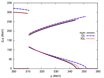
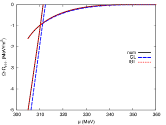
Figure 1: Comparison of the numerical results with the GL expansion and the IGL approximation for the CDW modulation as a function of the quark chemical potential. Top: values of $\Delta$ (curves with a decreasing behavior) and $q$ (curves with an increasing behavior) that minimize the free energy. Both GL and IGL give good results in the inhomogeneous phase. The GL tends to favor more the inhomogeneous phase over the chirally restored phase and in the homogenous $\chi$SB phase the GL expansion tends to overestimate $\Delta$. Bottom: free energy (after subtraction of the free energy of the chirally restored phase, $\Omega_{\text{rest}}$). The approximate expressions almost overlap with the numerical ones in the inhomogeneous $\chi$SB phase. However, in the homogenous $\chi$SB phase only the IGL approximation leads to a good agreement with the numerical results.

The first remarkable result visible by inspecting Fig. 1 is that even at zero temperature the standard GL expansion provides a good quantitative agreement with the results of the full numerical computation. It fails, however, to properly reproduce the numerical results in two key regions: Close to the transition to the chirally restored phase, where it overshoots the transition point, and at the transition between the homogeneous and inhomogeneous $\chi$SB phases, failing to correctly reproduce the value of $\Delta$ in the homogeneous $\chi$SB phase and the transition point. On the other hand, the IGL exactly does what it is designed for: it improves the description of these two regions. Most notably, it exactly reproduces the free energy in the homogeneous phase and the transition to the inhomogeneous $\chi$SB phase. Moreover, it shifts the transition to the chirally restored phase closer to the numerical result.

It is important to stress that, close to the chiral restoration transition the IGL is designed for giving a systematic controlled improvement over the standard GL by the inclusion of higher order $|\nabla^{n}M|^{2}$ terms, which, as already discussed, can be straightforwardly extracted from Eq. (13). This is shown in Fig. 2, where we can see how the second-order transition is increasingly better described as we include higher order terms. In particular, we can see that to get a good qualitative agreement we need at least the ${\cal{O}}(\alpha_{8})$ terms, otherwise the inhomogeneous $\chi$SB phase extends to arbitrarily high chemical potentials. We can interpret this result by inspecting Eq. (13), or equivalently the expressions for the GL coefficients: close to the chiral restoration transition and for reasonable values of $\mu/\Lambda$, the leading ${\cal{O}}(\alpha_{4})$ coefficient is negative and provides an energy gain in the formation of an inhomogeneous phase, whereas higher order terms constitute energy costs. Indeed, while we find that in principle within our regularization scheme the coefficients $\alpha_{4n}$ for $n>1$ might flip sign (see Eq. (II)) and actually favor large $q$ solutions, in practice this would require chemical potentials too close to the regulator $\Lambda$ for us to trust the model results in that regime. Therefore, we find that higher order gradient terms provide (increasingly smaller) energy costs which gradually push the phase transition towards lower chemical potentials, gradually approaching the full numerical result. In practice the convergence of this sum turns out to be very rapid: by including $\tilde{\alpha}_{10}$ corrections we are off the full numerical result for the transition chemical potential by only 2 MeV, and the IGL results from order $\tilde{\alpha}_{12}$ on become practically indistinguishable from the numerical result. In light of this, in the following we will consider for simplicity the truncated IGL expansion at order $\tilde{\alpha}_{10}$, with the understanding that more refined results can be straightforwardly obtained by simply adding higher order gradient terms.

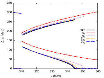
Figure 2: Analysis of the IGL approximation for the CDW condensate. The various lines correspond to the values of $\Delta$ (curves with a decreasing behavior) and $q$ (curves with an increasing behavior) that minimize the free energy, as a function of the quark chemical potential. Solid lines are results obtained by the full diagonalization of the quark Hamiltonian, the others correspond to the IGL expansion, Eq. (II), including gradient terms of different orders. Increasing the number of the gradient terms, the position of the second order phase transition is increasingly well determined.

IV.2 Real Kink Crystal

The results with the CDW ansatz suggest that the IGL approximation works extremely well. As a second check we compare the GL and IGL results with the numerical ones for the modulation which has been found to be the most favored in the inhomogeneous $\chi$SB window, namely the real kink crystal (RKC) Nickel (2009b); Buballa and Carignano (2015)

$$M(z)=\Delta\sqrt{\nu}\,{\text{sn}}(\Delta z|\nu)\,,$$ (15)

where ${\text{sn}}(\Delta z|\nu)$ is a Jacobi elliptic function, whose shape is characterized by $\Delta$ and by the so-called elliptic modulus $\nu$.

After computing the cell averages over $M(z)$ and plugging them in the GL and IGL expression, we obtain the results shown in Fig. 3. Again, we find a good agreement of the GL result with the full computation, while the IGL provides a significant quantitative improvement, reproducing the full numerical results within a few percent error. In this case the effect of the first term in the IGL expansion in Eq. (II) is more evident. It forces the average value of the condensate to match the homogeneous value, sensibly improving the agreement with the numerical results. This effect is due to the fact that the RKC ansatz can be seen as a superposition on many different waves with different amplitudes. The long-wavelength amplitudes dominate close to the phase transition with the homogeneous $\chi$SB phase. On the other hand, for a CDW, there is one single spatial frequency $q$, which is large. Therefore in that case the IGL does not improve much with respect to the GL approximation close to this phase transition.

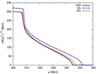
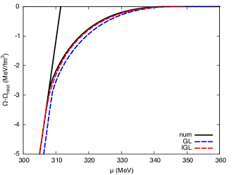
Figure 3: Comparison of the numerical results with the GL expansion and the IGL approximation for the RKC, Eq. (15). Top: average value of the condensate, $\sqrt{\langle M(z)^{2}\rangle}$. Bottom: difference between the free energy at the minimum and the free energy of the chirally restored phase.

It might be interesting at this point to compare the spatially modulated quark number density of the system obtained within the GL and IGL approximations with the numerical results of Carignano et al. (2010). In our case, it is simply obtained by differentiating the integrand of Eq. (II) with respect to $\mu$. This basically amounts to an improvement over a “local Fermi-gas” approximation (amounting to simply considering the first term in Eq. (II)), which has already been found to reproduce very well the behavior of the density of the system Buballa and Carignano (2016). Our results are shown in Fig. 4. There we can see that once again the IGL provides a better agreement with the full result as compared to the GL, although in this case the results do not match perfectly, especially close to the phase transition to the homogeneous broken phase. This is due to the fact that $\Delta$ and $\nu$ give the amplitude and frequency of the density oscillations. Since both are slightly different from the ones obtained by the full numerical calculation, the resulting density has amplitude and oscillation period different from the numerical ones.

The RKC modulation is somehow similar to the Lasagna phase in nuclear matter, that is a type of Pasta phase Ravenhall et al. (1983) expected to be realized in the inner crust of compact stars. In this phase nuclei form sheets immersed in a liquid of nuclear matter. However, with changing densities the Lasagna phase is supposed to be superseded by different modulations, possibly giving rise to higher-dimensional structures. Following this analogy one might expect that higher dimensional modulations can become favored at different values of the quark chemical potential. Another argument in favor of higher-dimensional modulations comes from quarkyonic matter studies, where it is expected that increasingly complex crystalline structures can be formed by the chiral condensate as the density increases Kojo et al. (2012).

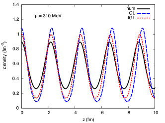
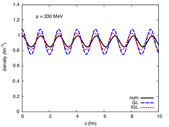
Figure 4: Comparison of the quark number density obtained by the GL, IGL and numerical methods for the RKC modulation (15). The IGL always performs better than the GL, with a discrepancy with the numerical method that is larger close to the $\chi$SB phase than at the chirally restored phase. The top panel correspond to $\mu=310$ MeV, while the bottom panel is obtained for $\mu=330$ MeV.

V Two-dimensional structures

Since the IGL provides very accurate results for the order parameters and free energies of one-dimensional modulations with minimal computational effort, let us now move on and consider two-dimensional structures. Close to the Lifshitz point, a systematic GL analysis of different types of higher dimensional modulations has been performed in Abuki et al. (2012), while a complementary numerical analysis for the astrophysical relevant $T=0$ case can be found in Carignano and Buballa (2012a). Comparing the IGL results with the numerical ones of Carignano and Buballa (2012a) for a two-dimensional square lattice with a sinusoidal ansatz, that is,

$$M(x,y)=\Delta\cos(qx)\cos(qy)\,,$$ (16)

we obtain the order parameters and the free energies reported in Fig. 5.

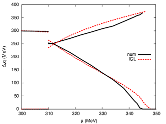
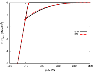
Figure 5: Comparison of the IGL and numerical methods for the 2D cosine modulation ansatz, see Eq. (16), as a function of the quark chemical potential. Top: Values of the order parameters $\Delta$ and $q$. Bottom: comparison of the free-energy difference $\Omega-\Omega_{\text{rest}}$.

It is clear that the agreement is again extremely good, and we recall that the IGL result can be computed with very limited numerical effort (basically amounting to the evaluation of $\langle\Omega_{\text{hom}}(\overline{M^{2}})\rangle$, as all the other terms can be computed analytically).

Using the IGL method we are in a position to easily test different 2D modulations. First we consider a square lattice with two RKC-type modulations along the $x$ and $y$ directions, that is

$$M(x,y)=\Delta\nu{\text{sn}}(\Delta x,\nu){\text{sn}}(\Delta y,\nu)\,.$$ (17)

The practical implementation of this modulation in the numerical framework of Carignano and Buballa (2012a) would be extremely complicated, as it would in principle require an expansion of the order parameter in a large number of Fourier harmonics and a minimization of the free energy with respect to all of their amplitudes. Instead, within the IGL approximation it can be straightforwardly implemented in the same way as with the 2D cosine. The minimization of the IGL free energy with respect to $\Delta$ and $\nu$ yields qualitatively similar results to the one-dimensional RKC for the order parameters. When computing the free energy associated with this modulation we find, similarly to what happens with the one-dimensional modulations, that the RKC-type solution is almost degenerate with the cosine one with the exception of the region close to the onset of the inhomogeneous phase, as shown in Fig. 6. In that figure we also see that this type of modulation is also disfavored with respect to its one-dimensional counterpart. We performed a further check in this direction by considering the ansatz

$$M(x,y)=\Delta\left[\sqrt{\nu_{x}}\,{\text{sn}}(\Delta x,\nu_{x})+\sqrt{\nu_{y}}\,{\text{sn}}(\Delta y,\nu_{y})\right]\,,$$ (18)

which can interpolate between a one-dimensional RKC modulation and a more involved two-dimensional structure. Consistent with our other results, we find that the minimum solution always corresponds to one of the two $\nu$ being zero, while the other reduces to the value obtained when minimizing with the one-dimensional ansatz Eq. (15).

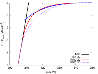
Figure 6: Comparison of the free energies for a 1D RKC (15), a 2D cosine (16) and a 2D RKC (17), within the IGL approximation.

Thus, as it was already found in Carignano and Buballa (2012a), we can confirm within our novel approach that 2D modulations are disfavored with respect to 1D modulations at vanishing temperatures. We therefore expect that the same “hierarchy” found in Abuki et al. (2012) close to the Lifshitz point holds also at vanishing temperatures, and that 3D modulations will thus be even further disfavored compared to two-dimensional ones.

VI Qualitative analysis of pairing

The comparison between the considered 2D modulations and the 1D modulations suggests that the 1D RKC is always favored. This result is in contrast with what is expected to occur in crystalline color superconductors, where a crystalline 3D pattern seems to be favored Alford et al. (2001); Mannarelli et al. (2006). It is believed that in color superconductors the occurrence of the crystalline phase is due to the maximization of pairing at the Fermi surface, indeed the presence of a collective Fermi surface phenomenon seems to be the key-point for obtaining a crystalline phase.

;       

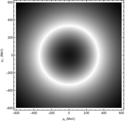
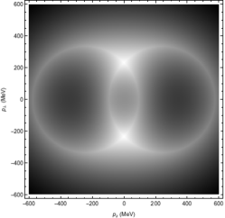
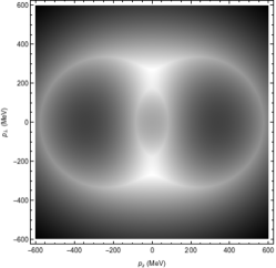
Figure 7: Two dimensional contour plots of the integrand of the free energy for CDW ansatz, Eq. (7). All the results are obtained for $\mu=335$ MeV, but different values of $q$ and $\Delta$. The lighter region corresponds to the region where the free energy cost for exciting quasiparticles is smaller. Left: unpaired phase, $q=0$ and $\Delta=0$. Center: $q=241$ MeV and $\Delta=0$. The effect of the large momentum $q$ is to strongly displace the Fermi spheres. Right: $q=241$ MeV and $\Delta=44$ MeV (corresponding to the energetically favored values at $\mu=335$ MeV). The smearing of the lighter region is due to the pairing.

Quite generally, a certain modulation is energetically favored if the energy gain due to pairing is larger than the energy cost of having pairs with nonvanishing total momentum. Let us examine in detail what happens in an inhomogeneous $\chi$SB condensate. For a qualitative understanding of the phenomenon we consider first the effect of a nonvanishing momentum and then we allow for pairing. For understanding whether multidimensional pairing is favored, we consider what happens for a plane wave ansatz. As discussed in Mannarelli et al. (2006); Anglani et al. (2014), one way of representing the Fermi surface effects is to inspect the integrand of the free energy, corresponding, in our case, to the integrand appearing in Eq. (7). In Fig. 7 we plot this function at $\mu=335$ MeV, that is within the inhomogeneous $\chi$SB window. The left panel corresponds to the free case, that is, $q=0$ and $\Delta=0$. The integrand is peaked at $p=\mu$, meaning that the larger contribution comes from the Fermi surface, corresponding to the lighter region in Fig. 7. This is the so-called pairing region, while the parts well inside the Fermi sphere or well outside it correspond to the blocking regions (see the discussion in Mannarelli et al. (2006) about pairing and blocking regions in color superconductors). In other words, pairing well inside/outside the Fermi sphere has a large free-energy cost, because particles should climb to the tip of the free energy (integrand), which is at the Fermi sphere. On the other hand, particle and hole excitations at the Fermi sphere are already at the tip of the mountain, that is to the largest possible energy, and they can eventually pair at no cost to form a chiral condensate Kojo et al. (2010).

Now we consider a momentum shift of the fermions. When pairs have nonvanishing total momentum, one can imagine first to displace fermions by $q$ and then to turn on pairing. This is exactly what one does when diagonalizes the full Hamiltonian for the single plane wave to obtain the free energy in Eq. (7). This procedure is discussed in detail in Mannarelli et al. (2006) for crystalline color superconductors, where it is shown how by a proper momentum shift the quark propagator becomes diagonal (see also Buballa and Carignano (2015) for an analogous discussion for inhomogeneous chiral condensates). This momentum shift has the effect of separating the Fermi spheres, as shown in the central panel of Fig. 7 for $q=241$ MeV. Now, the only pairing region corresponds to the ribbon where the two Fermi spheres touch. This picture also explains why $q<\mu$, indeed if this were not the case the two Fermi spheres would have no overlapping regions. Exciting quasiparticles and/or holes in the pairing ribbon has no free energy cost, whereas particles from all other regions should climb an energy barrier. Indeed, we see that this is exactly what happens for $\Delta=44$ MeV, right panel, where the smearing of the touching regions is exactly due to pairing. It is not possible now to add pairing in different regions of the Fermi spheres, say in the region $p_{\perp}\sim 0$, because these regions are too far apart and therefore the free energy cost for exciting particles and/or holes would be too high. Therefore, multidimensional modulations are disfavored in the $\chi$SB phase because $q$ is too large.

Figure 8: Contour plots of the integrand of the free energy for CDW ansatz, Eq. (7). For $\mu=335$ MeV, $q=30$ MeV and $\Delta=5$ MeV.

This does not happen in color superconductors. Indeed, one important difference between the inhomogeneous $\chi$SB phase and the crystalline color superconductors, regards the magnitude of $q$. Broadly speaking, $q$ has to be proportional to the stress exerted on the pairing mechanism. In the $\chi$SB phase the stress is proportional to $\mu$, because pairing is related to the formation of a chiral condensate. On the other hand, in color superconductors $q\propto\delta\mu$, where $\delta\mu\ll\mu$ is the mismatch between the Fermi spheres due to an unbalance between quarks of different flavors. For illustrative purposes, let us consider the non-energetically-favored $\chi$SB configuration corresponding to small $q$ and $\Delta$, somehow mimicking what happens in color superconductors. We show in Fig. 8 the integrand of Eq. (7), with $q=30$ MeV and $\Delta=5$ MeV. Again, pairing can happen in the ribbon where the two Fermi spheres overlap. However, it is clear now that it would be possible to slightly modify the Fermi sphere for allowing pairing, say in the $p_{\perp}\sim 0$ plane, at a small free-energy cost.

VII Conclusions

We have presented a novel approach to study spatially inhomogeneous pairing by an improved Ginzburg-Landau expansion, Eq. (II). This approach relies on a scale separation between long-wavelength fluctuations, dominating the transition to the homogeneous phase, and rapid fluctuations governing the transition to the chirally restored phase. The IGL reproduces correctly by construction the homogeneous limit and allows for a description of the chiral restoration transition from the inhomogeneous phase with arbitrarily high precision by a controlled gradient expansion.

We have applied the IGL to the study of the inhomogeneous $\chi$SB phase at $T=0$, reproducing the results obtained by numerical methods and extending the analysis to novel structures. These structures can hardly be studied by the numerical method, because of the complicated Fourier expansion technique underlying these methods. On the other hand, the IGL expansion turns out to be an extremely powerful tool, allowing us to quickly examine various crystalline structures to an arbitrarily accurate approximation. In this way we checked that various 2D modulations are disfavored with respect to the 1D RKC one in Eq. (15), confirming and extending previous results obtained via brute-force numerical computations Carignano and Buballa (2012a).

It is worth emphasizing that no approximate method so far has been used to analyze the $T=0$ case, probably because the standard GL approximation was assumed to be unreliable. Actually, we find that the GL approximation at the ${\cal O}(\alpha_{8})$ gives a surprisingly good qualitative agreement with the results of the full numerical computations. However, to make a quantitative comparison of the free energies of different structures a refined approach must be used, and the IGL devised here performs this task excellently. In particular, we showed that it is able to give an accurate description of both the second order phase transition to the chirally restored phase and of the phase transition to the homogeneous $\chi$SB phase. As it turns out, a small number of additional specific gradient terms is enough to provide an excellent agreement with the numerical data.

Finally, it is worth recalling that fluctuations are expected to have a strong effect on the formation of inhomogeneous condensates Lee et al. (2015); Yoshiike et al. (2017); Hidaka et al. (2015), particularly in the case of lower-dimensional modulations Landau and Lifshitz (1969) (see also Buballa and Carignano (2015) for a discussion). The inclusion of fluctuations in the IGL framework would lead to a systematic improvement beyond the mean-field approximation.

The present work can be extended in many different ways. The IGL free-energy can be used to rapidly evaluate the free energy of various crystalline color superconducting configurations, as the ones considered in Rajagopal and Sharma (2006), and to extend the analysis to novel modulations. The only modifications needed in Eq. (II) are the replacement of the free energy of the homogeneous phase with the 2SC one (for two flavors) or of the color flavor locked one (for three flavors) and to replace the $\alpha_{n}$ coefficients with the pertinent ones, which can in principle be obtained by considering modulations for which the eigenvalue spectrum is known, such as a simple Fulde-Ferrell type plane wave Fulde and Ferrell (1964); Larkin and Ovchinnikov (1964); Anglani et al. (2014). In this case one can also compare the IGL results with those obtained by the numerical method in Nickel and Buballa (2009). We will shortly present results on this topic.

Moreover, the IGL can be modified to simultaneously include the chiral and diquark condensates for examining the coexistence of the inhomogeneous $\chi$SB and of the crystalline color superconducting phase. In this case, the color-superconducting phase is expected to arise where the chiral condensate is small, or equivalently, where the density is large. Since 1D chiral modulations are favored, we expect that a cosine modulation, see for example Anglani et al. (2014), could be favored.

References

- Fukushima and Hatsuda (2011) K. Fukushima and T. Hatsuda, Rept.Prog.Phys. 74, 014001 (2011), eprint:1005.4814 [hep-ph] .
- Rajagopal and Wilczek (2000) K. Rajagopal and F. Wilczek, The Condensed Matter Physics of QCD (2000) arXiv:hep-ph/0011333 .
- Aarts (2013) G. Aarts, (2013), arXiv:1312.0968 [hep-lat] .
- Klevansky (1992) S. P. Klevansky, Rev. Mod. Phys. 64, 649 (1992).
- Buballa (2005) M. Buballa, Phys. Rept. 407, 205 (2005), eprint:hep-ph/0402234 .
- Anglani et al. (2014) R. Anglani, R. Casalbuoni, M. Ciminale, N. Ippolito, R. Gatto, et al., Rev.Mod.Phys. 86, 509 (2014), arXiv:1302.4264 [hep-ph] .
- Buballa and Carignano (2015) M. Buballa and S. Carignano, Prog. Part. Nucl. Phys. 81, 39 (2015), arXiv:1406.1367 [hep-ph] .
- Nickel (2009a) D. Nickel, Phys. Rev. Lett. 103, 072301 (2009a), arXiv:0902.1778 [hep-ph] .
- Alford et al. (1999) M. G. Alford, K. Rajagopal, and F. Wilczek, Nucl.Phys. B537, 443 (1999), arXiv:hep-ph/9804403 [hep-ph] .
- Rajagopal and Sharma (2006) K. Rajagopal and R. Sharma, Phys.Rev. D74, 094019 (2006), arXiv:hep-ph/0605316 [hep-ph] .
- Thies (2004) M. Thies, Phys. Rev. D69, 067703 (2004), arXiv:hep-th/0308164 [hep-th] .
- Nickel (2009b) D. Nickel, Phys.Rev. D80, 074025 (2009b), arXiv:0906.5295 [hep-ph] .
- Abuki et al. (2012) H. Abuki, D. Ishibashi, and K. Suzuki, Phys.Rev. D85, 074002 (2012), arXiv:1109.1615 [hep-ph] .
- Carignano and Buballa (2012a) S. Carignano and M. Buballa, Phys. Rev. D86, 074018 (2012a), arXiv:1203.5343 [hep-ph] .
- Nickel and Buballa (2009) D. Nickel and M. Buballa, Phys. Rev. D79, 054009 (2009), arXiv:0811.2400 .
- Mannarelli et al. (2006) M. Mannarelli, K. Rajagopal, and R. Sharma, Phys.Rev. D73, 114012 (2006), arXiv:hep-ph/0603076 [hep-ph] .
- Nambu and Jona-Lasinio (1961) Y. Nambu and G. Jona-Lasinio, Phys. Rev. 122, 345 (1961).
- Dautry and Nyman (1979) F. Dautry and E. Nyman, Nucl. Phys. A 319, 323 (1979).
- Nakano and Tatsumi (2005) E. Nakano and T. Tatsumi, Phys. Rev. D 71, 114006 (2005).
- Buballa and Carignano (2013) M. Buballa and S. Carignano, Phys. Rev D87, 054004 (2013), arXiv:1210.7155 [hep-ph] .
- Carignano and Buballa (2012b) S. Carignano and M. Buballa, Three days on quarkyonic islands. Proceedings, HIC for FAIR Workshop and 28th Max Born Symposium, Wroclaw, Poland, May 19-21, 2011, Acta Phys. Polon. Supp. 5, 641 (2012b), arXiv:1111.4400 [hep-ph] .
- Carignano et al. (2014) S. Carignano, M. Buballa, and B.-J. Schaefer, Phys. Rev. D90, 014033 (2014), arXiv:1404.0057 [hep-ph] .
- Carignano et al. (2010) S. Carignano, D. Nickel, and M. Buballa, Phys. Rev. D82, 054009 (2010), arXiv:1007.1397 .
- Buballa and Carignano (2016) M. Buballa and S. Carignano, Eur. Phys. J. A52, 57 (2016), arXiv:1508.04361 [nucl-th] .
- Ravenhall et al. (1983) D. G. Ravenhall, C. J. Pethick, and J. R. Wilson, Phys. Rev. Lett. 50, 2066 (1983).
- Kojo et al. (2012) T. Kojo, Y. Hidaka, K. Fukushima, L. D. McLerran, and R. D. Pisarski, Nucl. Phys. A 875, 94 (2012), eprint:1107.2124 [hep-ph] .
- Alford et al. (2001) M. G. Alford, J. A. Bowers, and K. Rajagopal, Phys.Rev. D63, 074016 (2001), arXiv:hep-ph/0008208 [hep-ph] .
- Kojo et al. (2010) T. Kojo, Y. Hidaka, L. McLerran, and R. Pisarski, Nucl. Phys. A 843, 37 (2010), eprint:0912.3800 [hep-ph] .
- Lee et al. (2015) T.-G. Lee, E. Nakano, Y. Tsue, T. Tatsumi, and B. Friman, Phys. Rev. D92, 034024 (2015), arXiv:1504.03185 [hep-ph] .
- Yoshiike et al. (2017) R. Yoshiike, T.-G. Lee, and T. Tatsumi, Phys. Rev. D95, 074010 (2017), arXiv:1702.01511 [hep-ph] .
- Hidaka et al. (2015) Y. Hidaka, K. Kamikado, T. Kanazawa, and T. Noumi, Phys. Rev. D 92, 034003 (2015), eprint:1505.00848 [hep-ph] .
- Landau and Lifshitz (1969) L. D. Landau and E. M. Lifshitz, Statistical physics Part 1, Course of theoretical physics (Pergamon, 1969).
- Fulde and Ferrell (1964) P. Fulde and R. A. Ferrell, Phys. Rev. 135, A550 (1964).
- Larkin and Ovchinnikov (1964) A. I. Larkin and Y. N. Ovchinnikov, Zh. Eksp. Teor. Fiz. 47, 1136 (1964), sov. Phys. JETP 20 762 (1965).