Video Enhancement with Task-Oriented Flow

Abstract

Many video enhancement algorithms rely on optical flow to register frames in a video sequence. Precise flow estimation is however intractable; and optical flow itself is often a sub-optimal representation for particular video processing tasks. In this paper, we propose task-oriented flow (TOFlow), a motion representation learned in a self-supervised, task-specific manner. We design a neural network with a trainable motion estimation component and a video processing component, and train them jointly to learn the task-oriented flow. For evaluation, we build Vimeo-90K, a large-scale, high-quality video dataset for low-level video processing. TOFlow outperforms traditional optical flow on standard benchmarks as well as our Vimeo-90K dataset in three video processing tasks: frame interpolation, video denoising/deblocking, and video super-resolution.

1 Introduction

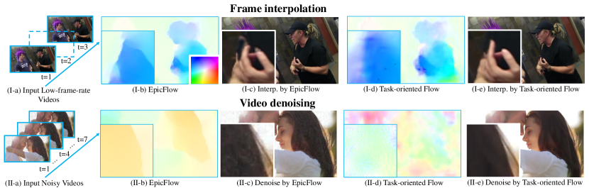
Figure 1: Many video processing tasks, e.g., temporal frame-interpolation (top) and video denoising (bottom), rely on flow estimation. In many cases, however, precise optical flow estimation is intractable and could be suboptimal for a specific task. For example, although EpicFlow (Revaud et al, 2015) predicts precise movement of objects (I-b, the flow field aligns well with object boundaries), small errors in estimated flow fields result in obvious artifacts in interpolated frames, like the obscure fingers in (I-c). With the task-oriented flow proposed in this work (I-d), those interpolation artifacts disappear as in (I-e). Similarly, in video denoising, our task-oriented flow (II-d) deviates from EpicFlow (II-b), but leads to a cleaner output frame (II-e). Flow visualization is based on the color wheel shown on the corner of (I-b).

Motion estimation is a key component in video processing tasks such as temporal frame interpolation, video denoising, and video super-resolution. Most motion-based video processing algorithms use a two-step approach (Liu and Sun, 2011; Baker et al, 2011; Liu and Freeman, 2010): they first estimate motion between input frames for frame registration, and then process the registered frames to generate the final output. Therefore, the accuracy of flow estimation greatly affects the performance of these two-step approaches.

However, precise flow estimation can be challenging and slow for many video enhancement tasks. The brightness constancy assumption, which many motion estimation algorithms rely on, may fail due to variations in lighting and pose, as well as the presence of motion blur and occlusion. Also, many motion estimation algorithms involve solving a large-scale optimization problem, making it inefficient for real-time applications.

Moreover, solving for a motion field that matches objects in motion may be sub-optimal for video processing. Figure 1 shows an example in frame interpolation. EpicFlow (Revaud et al, 2015), one of the state-of-the-art motion estimation algorithms, calculates a precise motion field (I-b) whose boundary is well-aligned with the fingers in the image (I-c); however, the interpolated frame (I-c) based on it still contains obvious artifacts due to occlusion. This is because EpicFlow only matches the visible parts between the two frames; however, for interpolation we also need to inpaint the occluded regions, where EpicFlow cannot help. In contrast, task-oriented flow, which we will soon introduce, learns to handle occlusions well (I-e), though its estimated motion field (I-d) differs from the ground truth optical flow. Similarly, in video denoising, EpicFlow can only estimate the movement of the girl’s hair (II-b), but our task-oriented flow (II-d) can remove the noise in the input. Therefore, the frame denoised by ours is much cleaner than that by EpicFlow (II-e). For specific video processing tasks, there exist motion representations that do not match the actual object movement, but lead to better results.

In this paper, we propose to learn this task-oriented flow (TOFlow) representation with an end-to-end trainable convolutional network that performs motion analysis and video processing simultaneously. Our network consists of three modules: the first estimates the motion fields between input frames; the second registers all input frames based on estimated motion fields; and the third generates target output from registered frames. These three modules are jointly trained to minimize the loss between output frames and ground truth. Unlike other flow estimation networks (Ranjan and Black, 2017; Fischer et al, 2015), the flow estimation module in our framework predicts a motion field tailored to a specific task, e.g., frame interpolation or video denoising, as it is jointly trained with the corresponding video processing module.

Several papers have incorporated a learned motion estimation network in burst processing (Tao et al, 2017; Liu et al, 2017). In this paper, we move beyond to demonstrate not only how joint learning helps, but also why it helps. We show that a jointly trained network learns task-specific features for better video processing. For example, in video denoising, our TOFlow learns to reduce the noise in the input, while traditional optical flow keeps the noisy pixels in the registered frame. TOFlow also reduces artifacts near occlusion boundaries. Our goal in this paper is to build a standard framework for better understanding when and how task-oriented flow works.

To evaluate the proposed TOFlow, we have also built a large-scale, high-quality video dataset for video processing. Most existing large video datasets, such as Youtube-8M (Abu-El-Haija et al, 2016), are designed for high-level vision tasks like event classification. The videos are often of low resolutions with significant motion blurs, making them less useful for video processing. We introduce a new dataset, Vimeo-90K, for a systematic evaluation of video processing algorithms. Vimeo-90K consists of 89,800 high-quality video clips (i.e. 720p or higher) downloaded from Vimeo. We build three benchmarks from these videos for interpolation, denoising or deblocking, and super-resolution, respectively. We hope these benchmarks will also help improve learning-based video processing techniques with their high-quality videos and diverse examples.

This paper makes three contributions. First, we propose TOFlow, a flow representation tailored to specific video processing tasks, significantly outperforming standard optical flow. Second, we propose an end-to-end trainable video processing framework that handles frame interpolation, video denoising, and video super-resolution. The flow network in our framework is fine-tuned by minimizing a task-specific, self-supervised loss. Third, we build a large-scale, high-quality video processing dataset, Vimeo-90K.

2 Related Work

Optical flow estimation. Dated back to Horn and Schunck (1981), most optical flow algorithms have sought to minimize hand-crafted energy terms for image alignment and flow smoothness (Mémin and Pérez, 1998; Brox et al, 2004, 2009; Wedel et al, 2009). Current state-of-the-art methods like EpicFlow (Revaud et al, 2015) or DC Flow (Xu et al, 2017) further exploit image boundary and segment cues to improve the flow interpolation among sparse matches. Recently, end-to-end deep learning methods were proposed for faster inference (Fischer et al, 2015; Ranjan and Black, 2017; Yu et al, 2016). We use the same network structure for motion estimation as SpyNet (Ranjan and Black, 2017). But instead of training it to minimize the flow estimation error, as SpyNet does, we train it jointly with a video processing network to learn a flow representation that is the best for a specific task.

Low-level video processing. We focus on three video processing tasks: frame interpolation, video denoising, and video super-resolution. Most existing algorithms in these areas explicitly estimate the dense correspondence among input frames, and then reconstruct the reference frame according to image formation models for frame interpolation (Baker et al, 2011; Werlberger et al, 2011; Yu et al, 2013; Jiang et al, 2018; Sajjadi et al, 2018), video super-resolution (Liu and Sun, 2014; Liao et al, 2015), and denoising (Liu and Freeman, 2010; Varghese and Wang, 2010; Maggioni et al, 2012; Mildenhall et al, 2018; Godard et al, 2017). We refer readers to survey articles (Nasrollahi and Moeslund, 2014; Ghoniem et al, 2010) for comprehensive literature reviews on these flourishing research topics.

Deep learning for video enhancement. Inspired by the success of deep learning, researchers have directly modeled enhancement tasks as regression problems without representing motions, and have designed deep networks for frame interpolation (Mathieu et al, 2016; Niklaus et al, 2017a; Jiang et al, 2017; Niklaus and Liu, 2018), super-resolution (Huang et al, 2015; Kappeler et al, 2016; Tao et al, 2017; Bulat et al, 2018; Ahn et al, 2018; Jo et al, 2018), denoising Mildenhall et al (2018), deblurring Yang et al (2018); Aittala and Durand (2018), rain drops removal (Li et al, 2018), and video compression artifacts removal (Lu et al, 2018).

Recently, with differentiable image sampling layers in deep learning (Jaderberg et al, 2015), motion information can be incorporated into networks and trained jointly. Such approaches have been applied to video interpolation (Liu et al, 2017), light-field interpolation (Wang et al, 2017), novel view synthesis (Zhou et al, 2016), eye gaze manipulation (Ganin et al, 2016), object detection (Zhu et al, 2017), denoising (Wen et al, 2017), and super-resolution (Caballero et al, 2017; Tao et al, 2017; Makansi et al, 2017). Although many of these algorithms also jointly train the flow estimation with the rest parts of network, there is no systematical study on the advantage of joint training. In this paper, we illustrate the advantage of the trained task-oriented flow through toy examples, and also demonstrate its superiority over general flow algorithm on various real-world tasks. We also present a general framework that can easily adapt to different video processing tasks.

3 Tasks

In the paper, we explore three video enhancement tasks: frame interpolation, video denoising/deblocking, and video super-resolution.

Temporal frame interpolation. Given a low frame rate video, a temporal frame interpolation algorithm generates a high frame rate video by synthesizing additional frames between two temporally neighboring frames. Specifically, let $I_{1}$ and $I_{3}$ be two consecutive frames in an input video, the task is to estimate the missing middle frame $I_{2}$. Temporal frame interpolation doubles the video frame rate, and can be recursively applied to generate even higher frame rates.

Video denoising/deblocking. Given a degraded video with artifacts from either the sensor or compression, video denoising/deblocking aims to remove the noise or compression artifacts to recover the original video. This is typically done by aggregating information from neighboring frames. Specifically, Let $\{I_{1},I_{2},\dots,I_{N}\}$ be $N$ consecutive, degraded frames in an input video, the task of video denoising is to estimate the middle frame $I_{\text{ref}}^{*}$. For the ease of description, in the rest of paper, we simply call both tasks as video denoising.

Video super-resolution. Similar to video denoising, given $N$ consecutive low-resolution frames as input, the task of video super-resolution is to recover the high-resolution middle frame. In this work, we first upsample all the input frames to the same resolution as the output using bicubic interpolation, and our algorithm only needs to recover the high-frequency component in the output image.

4 Task-Oriented Flow for Video Processing

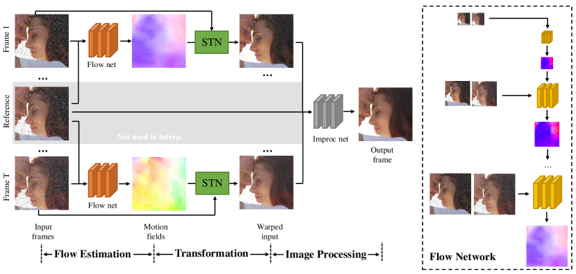
Figure 2: Left: our model using task-oriented flow for video processing. Given an input video, we first calculate the motion between frames through a task-oriented flow estimation network. We then warp input frames to the reference using spatial transformer networks, and aggregate the warped frames to generate a high-quality output image. Right: the detailed structure of flow estimation network (the orange network on the left).

Most motion-based video processing algorithms has two steps: motion estimation and image processing. For example, in temporal frame interpolation, most algorithms first estimate how pixels move between input frames (frame 1 and 3), and then move pixels to the estimated location in the output frame (frame 2) (Baker et al, 2011). Similarly, in video denoising, algorithms first register different frames based on estimated motion fields between them, and then remove noises by aggregating information from registered frames.

In this paper, we propose to use task-oriented flow (TOFlow) to integrate the two steps, which greatly improves the performance. To learn task-oriented flow, we design an end-to-end trainable network with three parts (Figure 2): a flow estimation module that estimates the movement of pixels between input frames; an image transformation module that warps all the frames to a reference frame; and a task-specific image processing module that performs video interpolation, denoising, or super-resolution on registered frames. Because the flow estimation module is jointly trained with the rest of the network, it learns to predict a flow field that fits to a particular task.

4.1 Toy Example

Before discussing the details of network structure, we first start with two synthetic sequences to demonstrate why our TOFlow can outperform traditional optical flows. The left of Figure 3 shows an example of frame interpolation, where a green triangle is moving to the bottom in front of a black background. If we warp both the first and the third frames to the second, even using the ground truth flow (Case I, left column), there is an obvious doubling artifact in the warped frames due to occlusion (Case I, middle column, top two rows), which is a well-known problem in the optical flow literature (Baker et al, 2011). The final interpolation result based on these two warp frames still contains the doubling artifact (Case I, right column, top row). In contrast, TOFlow does not stick to object motion: the background should be static, but it has non-zero motion (Case II, left column). With TOFlow, however, there is barely any artifact in the warped frames (Case II, middle column) and the interpolated frame looks clean (Case II, right column). This is because TOFlow not only synthesize the movement of visible object, but also guide how to inpaint occluded background region by copying pixels from its neighborhood. Also, if the ground truth occlusion mask is available, the interpolation result using ground truth flow will also contain little doubling artifacts (Case I, bottom rows). However, calculating the ground occlusion mask is even harder task than estimate flow, as it also requires inferring the correct depth ordering. On the other side, TOFlow can handle occlusion and synthesize frames better than the ground truth flow without using ground truth occlusion masks and depth ordering information.

Similarly, on the right of Figure 3, we show an example of video denoising. The random small boxes in the input frames are synthetic noises. If we warp the first and the third frames to the second using the ground truth flow, the noisy patterns (random squares) remain, and the denoised frame still contains some noise (Case I, right column. There are some shadows of boxes on the bottom). But if we warp these two frames using TOFlow (Case II, left column), those noisy patterns are also reduced or eliminated (Case II, middle column), and the final denoised frame base on them contains almost no noise, even better than the result by denoising results with ground truth flow and occlusion mask (Case I, bottom rows). This also shows that TOFlow learns to reduce the noise in input frames by inpainting them with neighboring pixels, which traditional flow cannot do.

Now we discuss the details of each module as follows.

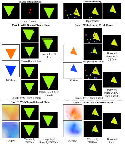
Figure 3: A toy example that demonstrates the effectiveness of task oriented flow over the traditional optical flow. See Section 4.1 for details.

4.2 Flow Estimation Module

The flow estimation module calculates the motion fields between input frames. For a sequence with $N$ frames ($N=3$ for interpolation and $N=7$ for denoising and super-resolution), we select the middle frame as the reference. The flow estimation module consists of $N-1$ flow networks, all of which have the same structure and share the same set of parameters. Each flow network (the orange network in Figure 2) takes one frame from the sequence and the reference frame as input, and predicts the motion between them.

We use the multi-scale motion estimation framework proposed by Ranjan and Black (2017) to handle the large displacement between frames. The network structure is shown in the right of Figure 2. The input to the network are Gaussian pyramids of both the reference frame and another frame rather than the reference. At each scale, a sub-network takes both frames at that scale and upsampled motion fields from previous prediction as input, and calculates a more accurate motion fields. We uses 4 sub-networks in a flow network, three of which are shown Figure 2 (the yellow networks).

There is a small modification for frame interpolation, where the reference frame (frame 2) is not an input to the network, but what it should synthesize. To deal with that, the motion estimation module for interpolation consists of two flow networks, both taking both the first and third frames as input, and predict the motion fields from the second frame to the first and the third respectively. With these motion fields, the later modules of the network can transform the first and the third frames to the second frame for synthesis.

4.3 Image Transformation Module

Using the predicted motion fields in the previous step, the image transformation module registers all the input frames to the reference frame. We use the spatial transformer networks (Jaderberg et al, 2015) (STN) for registration, which is a differentiable bilinear interpolation layer that synthesizes the new frame after transformation. Each STN transforms one input frame to the reference viewpoint, and all $N-1$ STNs forms the image transformation module. One important property of this module is that it can back-propagate the gradients from the image processing module to the flow estimation module, so we can learn a flow representation that adapts to different video processing tasks.

4.4 Image Processing Module

We use another convolutional network as the image processing module to generate the final output. For each task, we use a slightly different architecture. Please refer to appendices for details.

Occluded regions in warped frames. As mentioned Section 4.1, occlusion often results in doubling artifacts in the warped frames. A common way to solve this problem is to mask out occluded pixels in interpolation, for example, Liu et al (2017) proposed to use an additional network that estimates the occlusion mask and only uses pixels are not occluded.

Similar to Liu et al (2017), we also tried the mask prediction network. It takes the two estimated motion fields as input, one from frame 2 to frame 1, and the other from frame 2 to frame 3 ($v_{21}$ and $v_{23}$ in Figure 4). It predicts two occlusion masks: $m_{21}$ is the mask of the warped frame 2 from frame 1 ($I_{21}$), and $m_{23}$ is the mask of the warped frame 2 from frame 3 ($I_{23}$). The invalid regions in the warped frames ($I_{21}$ and $I_{23}$) are masked out by multiplying them with their corresponding masks. The middle frame is then calculated through another convolutional neural network with both the warped frames ($I_{21}$ and $I_{23}$) and the masked warped frames ($I_{21}^{\prime}$ and $I_{23}^{\prime}$) as input. Please refer to appendices for details.

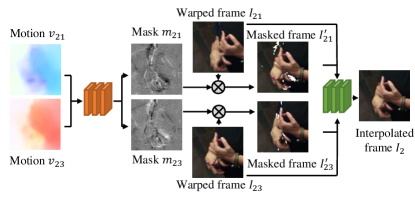
Figure 4: The structure of the mask network for interpolation

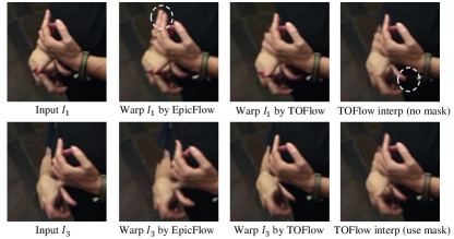
Figure 5: Comparison between Epicflow (Revaud et al, 2015) and TOFlow interpolation (both with and without mask).

An interesting observation is that, even without the mask prediction network, our flow estimation is mostly robust to occlusion. As shown in the third column of Figure 5, the warped frames using TOFlow has little doubling artifacts. Therefore, just from two warped frames without the learned masks, the network synthesizes a decent middle frame (the top image of the right most column). The mask network is optional, as it only removes some tiny artifacts.

4.5 Training

To accelerate the training procedure, we first pre-train some modules of the network and then fine-tune all of them together. Details are described below.

Pre-training the flow estimation network. Pre-training the flow network consists of two steps. First, for all tasks, we pre-train the motion estimation network on the Sintel dataset (Butler et al, 2012), a realistically rendered video dataset with ground truth optical flow.

In the second step, for video denoising and super-resolution, we fine-tune it with noisy or blurry input frames to improve its robustness to these input. For video interpolation, we fine-tune it with frames $I_{1}$ and $I_{3}$ from video triplets as input, minimizing the $l_{1}$ difference between the estimated optical flow and the ground truth flow $v_{23}$ (or $v_{21}$). This enables the flow network to calculate the motion from the unknown frame $I_{2}$ to frame $I_{3}$ given only frames $I_{1}$ and $I_{3}$ as input.

Empirically we find that this two-step pre-training can improve the convergence speed. Also, because the main purpose of pre-training is to accelerate the convergence, we simply use the $l_{1}$ difference between estimated optical flow and the ground truth as the loss function, instead of end-point error in flow literature (Brox et al, 2009; Butler et al, 2012). The choice loss function in the pre-training stage has a minor impact on the final result.

Pre-training the mask network. We also pre-train our occlusion mask estimation network for video interpolation as an optional component of video processing network before joint training. Two occlusion masks ($m_{21}$ and $m_{23}$) are estimated together with the same network and only optical flow $v_{21},v_{23}$ as input. The network is trained by minimizing the $l_{1}$ loss between the output masks and pre-computed occlusion masks.

Joint training. After pre-training, we train all the modules jointly by minimizing the $l_{1}$ loss between recovered frame and the ground truth, without any supervision on estimated flow fields. For optimization, we use ADAM (Kingma and Ba, 2015) with a weight decay of $10^{-4}$. We run 15 epochs with batch size 1 for all tasks. The learning rate for denoising/deblocking and super-resolution is $10^{-4}$, and the learning rate for interpolation is $3\times 10^{-4}$.

5 The Vimeo-90K Dataset

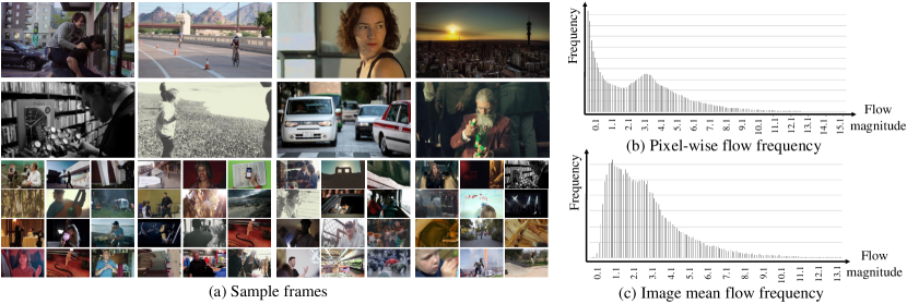
Figure 6: The Vimeo-90K dataset. (a) Sampled frames from the dataset, which show the high quality and wide coverage of our dataset; (b) The histogram of flow magnitude of all pixels in the dataset; (c) The histogram of mean flow magnitude of all images (the flow magnitude of an image is the average flow magnitude of all pixels in that image).

To acquire high quality videos for video processing, previous methods (Liu and Sun, 2014; Liao et al, 2015) took videos by themselves, resulting in video datasets that are small in size and limited in terms of content. Alternatively, we resort to Vimeo where many videos are taken with professional cameras on diverse topics. In addition, we only search for videos without inter-frame compression (e.g., H.264), so that each frame is compressed independently, avoiding artificial signals introduced by video codecs. As many videos are composed of multiple shots, we use a simple threshold-based shot detection algorithm to break each video into consistent shots and further use GIST feature (Oliva and Torralba, 2001) to remove shots with similar scene background.

As a result, we collect a new video dataset from Vimeo, consisting of 4,278 videos with 89,800 independent shots that are different from each other in content. To standardize the input, we resize all frames to the fixed resolution 448$\times$256. As shown in Figure 6, frames sampled from the dataset contain diverse content for both indoor and outdoor scenes. We keep consecutive frames when the average motion magnitude is between 1–8 pixels. The right column of Figure 6 shows the histogram of flow magnitude over the whole dataset, where the flow fields are calculated using SpyNet (Ranjan and Black, 2017).

We further generate three benchmarks from the dataset for the three video enhancement tasks studied in this paper.

Vimeo interpolation benchmark. We select 73,171 frame triplets from 14,777 video clips with the following three criteria for the interpolation task. First, more than 5% pixels should have motion larger than 3 pixels between neighboring frames. This criterion removes static videos. Second, $l_{1}$ difference between the reference and the warped frame using optical flow (calculated using SpyNet) should be at most 15 intensity levels (the maximum intensity level of an image is 255). This removes frames with large intensity change, which are too hard for frame interpolation. Third, the average difference between motion fields of neighboring frames ($v_{21}$ and $v_{23}$) should be less than 1 pixel. This removes non-linear motion, as most interpolation algorithms, including ours, are based on linear motion assumption.

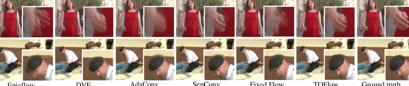
Figure 7: Qualitative results on frame interpolation. Zoomed-in views are shown in lower right.

Vimeo denoising/deblocking benchmark. We select 91,701 frame septuplets from 38,990 video clips for the denoising task, using the first two criteria introduced for the interpolation benchmark. For video denoising, we consider two types of noises: a Gaussian noise with a standard deviation of 0.1, and mixed noises including a 10$\%$ salt-and-pepper noise in addition to the Gaussian noise. For video deblocking, we compress the original sequences using FFmpeg with codec JPEG2000, format J2k, and quantization factor $q=\{20,40,60\}$.

Vimeo super-resolution benchmark. We also use the same set of septuplets for denoising to build the Vimeo super-resolution benchmark with down-sampling factor of 4: the resolution of input and output images are $112\times 64$ and $448\times 256$ respectively. To generate the low-resolution videos from high-resolution input, we use the MATLAB imresize function, which first blurs the input frames using cubic filters and then downsamples videos using bicubic interpolation.

6 Evaluation

In this section, we evaluate two variations of the proposed network. The first one is to train each module separately: we first pre-train motion estimation, and then train video processing while fixing the flow module. This is similar to the two-step video processing algorithms, and we refer to it as Fixed Flow. The other one is to jointly train all modules as described in Section 4.5, and we refer to it as TOFlow. Both networks are trained on Vimeo benchmarks we collected. We evaluate these two variations on three different tasks and also compare with other state-of-the-art image processing algorithms.

6.1 Frame Interpolation

Datasets. We evaluate on three datasets: Vimeo interpolation benchmark, the dataset used by Liu et al (2017) (DVF), and Middlebury flow dataset (Baker et al, 2011).

Metrics. We use two quantitative measure to evaluate the performance of interpolation algorithms: peak signal-to-noise ratio (PSNR) and structural similarity (SSIM) index.

Baselines. We first compare our framework with two-step interpolation algorithms. For the motion estimation, we use EpicFlow (Revaud et al, 2015) and SpyNet (Ranjan and Black, 2017). To handle occluded regions as mentioned in Section 4.4, we calculate the occlusion mask for each frame using the algorithm proposed by Zitnick et al (2004) and only use non-occluded regions to interpolate the middle frame. Further, we compare with state-of-the-art end-to-end models, Deep Voxel Flow (DVF) (Liu et al, 2017), Adaptive Convolution (AdaConv) (Niklaus et al, 2017a), and Separable Convolution (SepConv) (Niklaus et al, 2017b). At last, we also compare with Fixed Flow, which is another baseline two-step interpolation algorithm.

Methods	Vimeo Interp.		DVF Dataset
	PSNR	SSIM	PSNR	SSIM
SpyNet	31.95	0.9601	33.60	0.9633
EpicFlow	32.02	0.9622	33.71	0.9635
DVF	33.24	0.9627	34.12	0.9631
AdaConv	32.33	0.9568	—	—
SepConv	33.45	0.9674	34.69	0.9656
Fixed Flow	29.09	0.9229	31.61	0.9544
Fixed Flow + Mask	30.10	0.9322	32.23	0.9575
TOFlow	33.53	0.9668	34.54	0.9666
TOFlow + Mask	33.73	0.9682	34.58	0.9667

Table 1: Quantitative results of different frame interpolation algorithms on the Vimeo interpolation test set and the DVF test set (Liu et al, 2017).

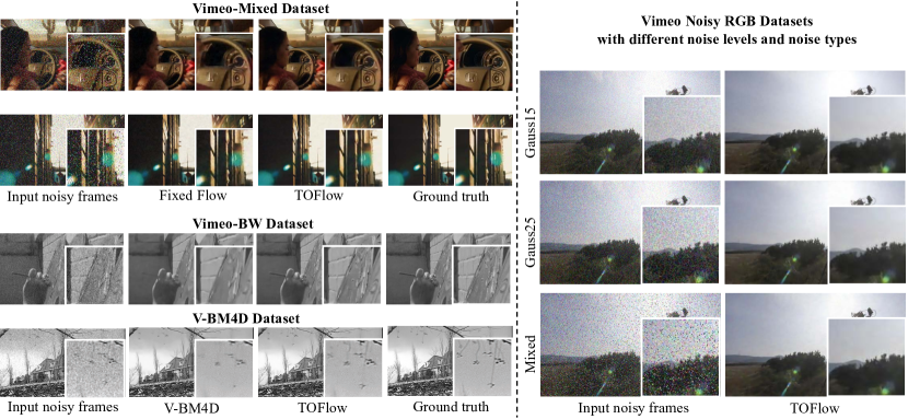
Figure 8: Qualitative results on video denoising. The differences are clearer when zoomed-in.

Results. Table 1 shows our quantitative results. On Vimeo interpolation benchmark, TOFlow in general outperforms the others interpolation algorithms, both the traditional two-step interpolation algorithms (EpicFlow and SpyNet) and recent deep-learning based algorithms (DVF, AdaConv, and SepConv), with a significant margin. Though our model is trained on our Vimeo-90K dataset, it also outperforms DVF on DVF dataset in both PSNR and SSIM. There is also a significant boost over Fixed Flow, showing that the network does learn a better flow representation for interpolation during joint training.

Figure 7 also shows qualitative results. All the two-step algorithms (EpicFlow and Fixed Flow) generate a doubling artifacts, like the hand in the first row or the head in the second row. AdaConv on the other sides does not have the doubling artifacts, but it tends to generate blurry output, by directly synthesizing interpolated frames without a motion module. SepConv increases the sharpness of output frame compared with AdaConv, but there are still artifacts (see the hat on the bottom row). Compared with these methods, TOFlow correctly recovers sharper boundaries and fine details even in presence of large motion.

Table 2 shows a qualitative comparison of the proposed algorithms with the best four alternatives on Middlebury (Baker et al, 2011). We use the sum of square difference (SSD) reported on the official website as the evaluation metric. TOFlow performs better than other interpolation networks.

Methods	PMMST	DeepFlow	SepConv	TOFlow	TOFlow
					Mask
All	5.783	5.965	5.605	5.67	5.49
Discontinuous	9.545	9.785	8.741	8.82	8.54
Untextured	2.101	2.045	2.334	2.20	2.17

Table 2: Quantitative results of five frame interpolation algorithms on Middlebury flow dataset (Baker et al, 2011): PMMST (Xu et al, 2015), SepConv (Niklaus et al, 2017b), DeepFlow (Liu et al, 2017), and our TOFlow (with and without mask). Follow the convention of Middlebury flow dataset, we reported the square root error (SSD) between ground truth image and interpolated image in 1) entire images, 2) regions of motion discontinuities, and 3) regions without texture.

Methods	Vimeo-Gauss15		Vimeo-Gauss25		Vimeo-Mixed
	PSNR	SSIM	PSNR	SSIM	PSNR	SSIM
Fixed Flow	36.25	0.9626	34.74	0.9411	31.85	0.9089
TOFlow	36.63	0.9628	34.89	0.9518	33.51	0.9395

Methods	Vimeo-BW		V-BM4D
	PSNR	SSIM	PSNR	SSIM
V-BM4D	33.17	0.8756	30.63	0.8759
TOFlow	36.75	0.9275	30.36	0.8855

Table 3: Quantitative results on video denoising. Left: Vimeo RGB datasets with three different types of noise; Right: two grayscale dataset: Vimeo-BW and V-BM4D.

6.2 Video Denoising/Deblocking

Setup. We first train and evaluate our framework on Vimeo denoising benchmark, with three types of noises: Gaussian noise with standard deviation of 15 intensity levels (Vimeo-Gauss15), Gaussian noise with standard deviation of 25 (Vimeo-Gauss25), and mixture of Gaussian noise and 10% salt-and-pepper noise (Vimeo-Mixed). To compare our network with V-BM4D (Maggioni et al, 2012), which is a monocular video denoising algorithm, we also transfer all videos in Vimeo Denoising Benchmark to grayscale to create Vimeo-BW (Gaussian noise only), and retrain our network on it. We also evaluate our framework on the a mono video dataset in V-BM4D.

Baselines. We compare our framework with the V-BM4D, with the standard deviation of Gaussian noise as its additional input on two grayscale datasets (Vimeo-BW and V-BM4D). As before, we also compare with the Fixed Flow variant of our framework on three RGB datasets (Vimeo-Gauss15, Vimeo-Gauss25, and Vimeo-Mixed).

Methods	Vimeo-Blocky (q=20)		Vimeo-Blocky (q=40)		Vimeo-Blocky (q=60)
	PSNR	SSIM	PSNR	SSIM	PSNR	SSIM
V-BM4D	35.75	0.9587	33.72	0.9402	32.67	0.9287
Fixed flow	36.52	0.9636	34.50	0.9485	33.06	0.9168
TOFlow	36.92	0.9663	34.97	0.9527	34.02	0.9447

Table 4: Results on video deblocking.

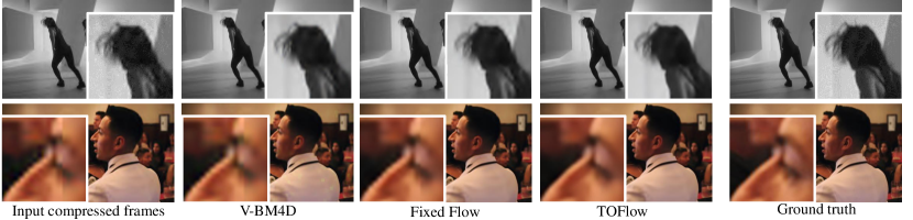
Figure 9: Qualitative results on video deblocking. The differences are clearer when zoomed-in.

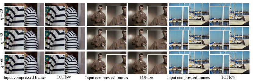
Figure 10: Results on frames with different encoding qualities. The differences are clearer when zoomed-in.

Results. We first evaluate TOFlow on the Vimeo dataset with three different noise levels (Table 3). TOFlow outperforms Fixed Flow by a significant margin, demonstrating the effectiveness of joint training. Also, when the noise level increases to 25 or when additional salt-and-pepper noise is added, the PSNR of TOFlow is still round 34dB, showing its robustness to different noise levels. This is qualitatively demonstrated in the right half of Figure 8.

On two grayscale datasets, Vimeo-BW and V-BM4D, TOFlow outperforms V-BM4D in SSIM. Here we do not fine-tune it on V-BM4D. Though TOFlow only achieves a comparable performance with V-BM4D in PSNR, the output of TOFlow is much sharper than V-BM4D. As shown in Figure 8, the details of the beard and collar are kept in the denoised frame by TOFlow (the mid left of Figure 8), and leaves on the tree are also clearer (the bottom left of Figure 8). Therefore, TOFlow beats V-BM4D in SSIM, which better reflects human’s perception than PSNR.

For video deblocking, Table 4 shows that TOFlow outperforms V-BM4D. Figure 9 also shows the qualitative comparison between TOFlow, Fixed Flow, and V-BM4D. Note that the compression artifacts around the girl’s hair (top) and the man’s nose (bottom) are completely removed by TOFlow. The vertical line around the man’s eye (bottom) due to a blocky compression is also removed by our algorithm. To demonstrate the robustness of our algorithms on video deblocking with different quantization levels, we also evaluate the three algorithms on input videos generated under three different quantization levels, and TOFlow consistently outperforms other two baselines. Figure 10 also shows that when the quantization level increases, the deblocking output remains mostly the same, suggesting the robustness of TOFlow.

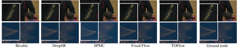
Figure 11: Qualitative results on super-resolution. Close-up views are shown on the top left of each result. The differences are clearer when zoomed-in.

6.3 Video Super-Resolution

Datasets. We evaluate our algorithm on two dataset: Vimeo super-resolution benchmark and the dataset provided by Liu and Sun (2011) (BayesSR). The later one consists of four sequences, each having 30 to 50 frames. Vimeo super-resolution benchmark only contains 7 frames, so there is no full-clip evaluation for it.

Baselines. We compare our framework with bicubic up-sampling, three video SR algorithms: BayesSR (we use the version provided by Ma et al (2015)), DeepSR (Liao et al, 2015), and SPMC (Tao et al, 2017), as well as a baseline with a Fixed Flow estimation module. Both BayesSR and DeepSR can take various number of frames as input. Therefore, on BayesSR dataset, we report two numbers: one on the whole sequence, the other on the seven frames in the middle, as SPMC, TOFlow, and Fixed Flow only take 7 frames as input.

Input	Methods	Vimeo-SR		BayesSR
		PSNR	SSIM	PSNR	SSIM
Full Clip	DeepSR	—	—	22.69	0.7746
	BayesSR	—	—	24.32	0.8486
1 Frame	Bicubic	29.79	0.9036	22.02	0.7203
7 Frames	DeepSR	25.55	0.8498	21.85	0.7535
	BayesSR	24.64	0.8205	21.95	0.7369
	SMPC	32.70	0.9380	21.84	0.7990
	Fixed Flow	31.81	0.9288	22.85	0.7655
	TOFlow	33.08	0.9417	23.54	0.8070

Table 5: Results on video super-resolution. Each clip in Vimeo-SR contains 7 frames, and each clip in BayesSR contains 30–50 frames.

3 Frames		5 Frames		7 Frames
PSNR	SSIM	PSNR	SSIM	PSNR	SSIM
32.66	0.9375	33.04	0.9415	33.08	0.9417

Table 6: Results on video super-resolution with a different number of input frames.

Cubic Kernel		Box Kernel		Gaussian Kernel
PSNR	SSIM	PSNR	SSIM	PSNR	SSIM
33.08	0.9417	32.08	0.9372	31.15	0.9314

Table 7: Results of TOFlow on video super-resolution when different downsampling kernels are used for building the dataset.

Results. Table 5 shows our quantitative results. Our algorithm performs better than baseline algorithms when using 7 frames as input, and it also achieves comparable performance to BayesSR when BayesSR uses all 30–50 frames as input while our framework only uses 7 frames. We show qualitative results in Figure 11. Compared with either DeepSR or Fixed Flow, the jointly trained TOFlow generates sharper output. Notice the text on the cloth (top) and the tip of the knife (bottom) are clearer in the high-resolution frame synthesized by TOFlow. This shows the effectiveness of joint training.

To better understand how many input frames are sufficient for super-resolution, we also train our TOFlow with different number of input frames, as shown in Table 6. There is a big improvement when switching from 3-frame to 5-frame, and the improvement becomes minor when further switching to 7-frame. Therefore, 5 or 7 frames should be enough for super-resolution.

Besides, the down-sampling kernels (a.k.a. the point-spread function) used to create the low-resolution images may also affect the performance super-resolution (Liao et al, 2015). To evaluate how down-sampling kernels affect the performance of our algorithm, we evaluate on three different kernels: cubic kernels, box down-sampling kernels, and Gaussian kernels with a variance of 2 pixels), and Table 7 shows the result. There is a 1 dB drop in PSNR when switching to box kernels, and another 1 dB drop when switching to Gaussian kernels. This is because that down-sampling kernels remove high-frequency aliasing in low-resolution input images, making super-resolution harder. In most of experiments here, we follow the convention in previous multi-frame super-solution papers (Liu and Sun, 2011; Tao et al, 2017), which creates low-resolution images through bicubic interpolation with no blur kernels. However, the results with blur kernels are also interesting, as it is closer the actual formation of low-resolution images captured by cameras.

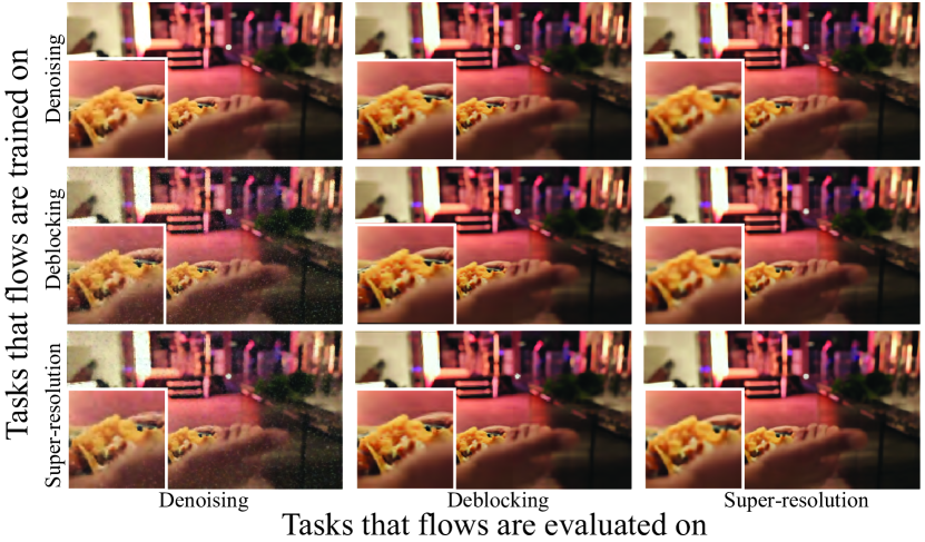
Figure 12: Qualitative results of TOFlow on tasks including but not limited to the one it was trained on.

In all the experiments, we train and evaluate our network on an NVIDIA Titan X GPU. For an input clip with resolution $256\times 448$, our network takes about 200ms for interpolation and 400ms for denoising or super-resolution (the resolution of the input to the super-resolution network is $64\times 112$), where the flow module takes 18 ms for each estimated motion field.

Figure 13: Visualization of motion fields for different tasks.

6.4 Flows Learned from Different Tasks

We now compare and contrast the flow learned from different tasks to understand if learning flow in such a task-oriented fashion is necessary.

We conduct an ablation study by replacing the flow estimation network in our model by a flow network trained on a different task (Figure 12 and Table 8). There is a significant performance drop when we use a flow network that is not trained on that task. For example, with the flow network trained on deblocking or super-resolution, the performance of the denoising algorithm drops by 5dB, and there are noticeable noises in the images (the first column of Figure 12). There are also ringing artifacts when we apply the flow network trained on super-resolution for deblocking (Figure 12 row 2, col 2). Therefore, our task-oriented flow network is indeed tailored to a specific task. Besides, in all these three tasks, Fixed Flow performs better than TOFlow if trained and tested on different tasks, but worse than TOFlow if trained and tested on the same task. This suggests that joint training improves the performance of a flow network on one task, but decreases its performance on the others.

Figure 13 contrasts the motion fields learned from different tasks: the flow field for interpolation is very smooth, even on the occlusion boundaries, while the flow field for super-resolution has artificial movements along the texture edges. This indicates that the network may learn to encode different information that is useful for different tasks in the learned motion fields.

Tasks trained on	Tasks evaluated on
	Denoising	Deblocking	Super-resolution
Denoising	34.89	36.13	31.30
Deblocking	25.74	36.92	31.86
Super-resolution	25.99	31.86	33.08
Fixed Flow	34.74	36.52	31.81
EpicFlow	30.43	30.09	28.05

Table 8: PSNR of TOFlow on tasks including but not limited to the one it was trained on.

6.5 Accuracy of Retrained Flow

As shown in the Figure 1, tailoring a motion estimation network to a specific task will reduce the accuracy of the estimated flow. To verify that, we evaluate the flow estimation accuracy on the Sintel Flow Dataset by Butler et al (2012). Three variants of flow estimation networks are tested: first, a network pre-trained on the Flying Chair dataset, second, the network after fine-tuning on denoising, and third, the network after fine-tuning on super-resolution. All fine-tuning is on the Vimeo-90K dataset. As shown in Table 9, the accuracy of TOFlow is much worse than either EpicFlow (Revaud et al, 2015) or Fixed Flow , but as shown in Table 3, 4, and 5, TOFlow outperforms Fixed Flow on specific tasks. This is consistent with the intuition that TOFlow is a motion representation that does not match the actual object movement, but leads to better video processing results.

Methods	TOFlow	TOFlow	Fixed	Epic
	Denoising	Super-resolution	Flow	Flow
All	16.638	16.586	14.120	4.115
Matched	11.961	11.851	9.322	1.360
Unmatched	54.724	55.137	53.117	26.595

Table 9: End-point-error (EPE) of estimated flow fields on the Sintel dataset. We evaluate TOFlow (trained on two different tasks), Fixed Flow, and EpicFlow (Revaud et al, 2015). We report errors over full images, matched regions, and unmatched regions.

6.6 Different Flow Estimation Network Structure

Our task-oriented video processing pipeline is not limited to one flow estimation network structure, although in all previous experiments, we use SpyNet by Ranjan and Black (2017) as the flow estimation module for its memory efficiency. To demonstrate the generalization ability of our framework, we also experiment with the FlowNetC (Fischer et al, 2015) structure, and evaluate it on video denoising, deblocking, and super-resolution. Because FlowNetC has larger memory consumption, we only estimate flow at 256$\times$192 and upsample it to the target resolution. Its performance is therefore worse than the model using SpyNet, as shown in Table 10. Still, in all these three tasks, TOFlow outperforms than Fixed Flow. This demonstrates the generalization ability of the TOFlow framework to other flow estimation modules.

Methods	Denoising		Deblocking		Super-resolution
	PSNR	SSIM	PSNR	SSIM	PSNR	SSIM
Fixed Flow	24.685	0.8297	36.028	0.9672	31.834	0.9291
TOFlow	24.689	0.8374	36.496	0.9700	33.010	0.9411

Table 10: Results of TOFlow on three different tasks, using FlowNetC (Fischer et al, 2015) as the motion estimation module.

7 Conclusion

In this work, we have proposed a novel video processing model that exploits task-oriented motion cues. Traditional video processing algorithms normally consist of two steps: motion estimation and video processing based on estimated motion fields. However, a genetic motion for all tasks might be sub-optimal and the accurate motion estimation would be neither necessary nor sufficient for these tasks. Our self-supervised, task-oriented flow (TOFlow) bypasses this difficulty by modeling motion signals in the loop. To evaluate our algorithm, we have also created a new dataset, Vimeo-90K, for video processing. Extensive experiments on temporal frame interpolation, video denoising/deblocking, and video super-resolution demonstrate the effectiveness of TOFlow.

Acknowledgements. This work is supported by NSF RI #1212849, NSF BIGDATA #1447476, Facebook, Shell Research, and Toyota Research Institute. This work was done when Tianfan Xue and Donglai Wei were graduate students at MIT CSAIL.

Appendices

Additional qualitative results. We show additional results on the following benchmarks: Vimeo interpolation benchmark (Figure 14), Vimeo denoising benchmark (Figure 15 for RGB videos, and Figure 16 for grayscale videos), Vimeo deblocking benchmark (Figure 17), and Vimeo super-resolution benchmark (Figure 18). We randomly select testing images from test datasets. Differences between different algorithms are more clearer when zoomed in.

Flow estimation module. We use SpyNet (Ranjan and Black, 2017) as our flow estimation module. It consists of four sub-networks with the same network structure, but each sub-network has an independent set of parameters. Each sub-network consists of five sets of 7$\times$7 convolutional (with zero padding), batch normalization and ReLU layers. The number of channels after each convolutional layer is 32, 64, 32, 16, and 2. The input motion to the first network is a zero motion field.

Image processing module. We use slight different structures in the image processing module for different tasks. For temporal frame interpolation both with and without masks, we build a residual network that consists of an averaging network and a residual network. The averaging network simply averages the two transformed frames (from frame 1 and frame 3). The residual network also takes the two transformed frames as input, but calculates the difference between the actual second frame and the average of two transformed frames through a convolutional network consists of three convolutional layers, each of which is followed by a ReLU layer. The kernel sizes of three layers are 9$\times$9, 1$\times$1, and 1$\times$1 (with zero padding), and the numbers of output channels are 64, 64, and 3. The final output is the summation of the output of the averaging network and the residual network.

For video denoising/deblocking, the image processing module uses the same six-layer convolutional structure (three convolutional layers and three ReLU layers) as interpolation, but without the residual structure. We have also tried the residual structure for denoising/deblocking, but there is no significant improvement.

For video super-resolution, the image processing module consists of four pairs of convolutional layers and ReLU layers. The kernel sizes for these four layers are 9$\times$9, 9$\times$9, 1$\times$1, and 1$\times$1 (with zero padding), and the numbers of output channels are 64, 64, 64, and 3.

Mask network. Similar to our flow estimation module, our mask estimation network is also a four-level convolutional neural network pyramid as in Figure 4. Each level consists of the same sub-network structure with five sets of 7$\times$7 convolutional (with zero padding), batch normalization and ReLU layers, but an independent set of parameters (output channels are 32, 64, 32, 16, and 2). For the first level, the input to the network is a concatenation of two estimated optical flow fields (four channels after concatenation), and the output is a concatenation of two estimated masks (one channel per mask). From the second level, the input to the network switch to a concatenation of, first, two estimated optical flow fields at that resolution, and second, bilinear-upsampled masks from the previous level (the resolution is twice of the previous level). In this way, the first level mask network estimates a rough mask, and the rest refines high frequency details of the mask.

We use cycle consistencies to obtain the ground truth occlusion mask for pre-training the mask network. For two consecutive frames $I_{1}$ and $I_{2}$, we calculate the forward flow $v_{12}$ and the backward flow $v_{21}$ using the pre-trained flow network. Then, for each pixel $p$ in image $I_{1}$, we first map it to $I_{2}$ using $v_{12}$ and then map it back to $I_{1}$ using $v_{21}$. If it maps to a different point rather to $p$ (up to an error threshold of two pixels), then this point is considered to be occluded.

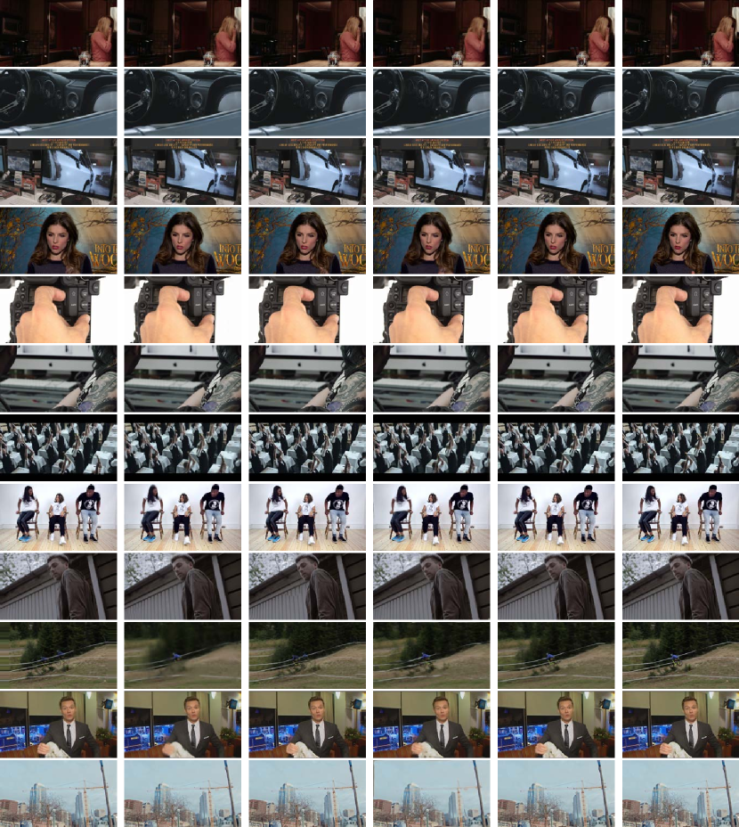
EpicFlow

AdaConv

SepConv

​Fixed Flow

TOFlow

​​​​​​ Ground Truth

Figure 14: Qualitative results on video interpolation. Samples are randomly selected from the Vimeo interpolation benchmark. The differences between different algorithms are clear only when zoomed in.

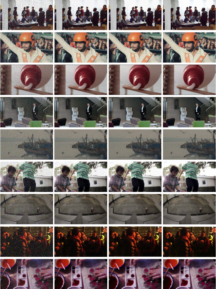
Input

​​Fixed Flow

TOFlow

Ground Truth

Figure 15: Qualitative results on RGB video denoising. Samples are randomly selected from the Vimeo denoising benchmark. The differences between different algorithms are clear only when zoomed in.

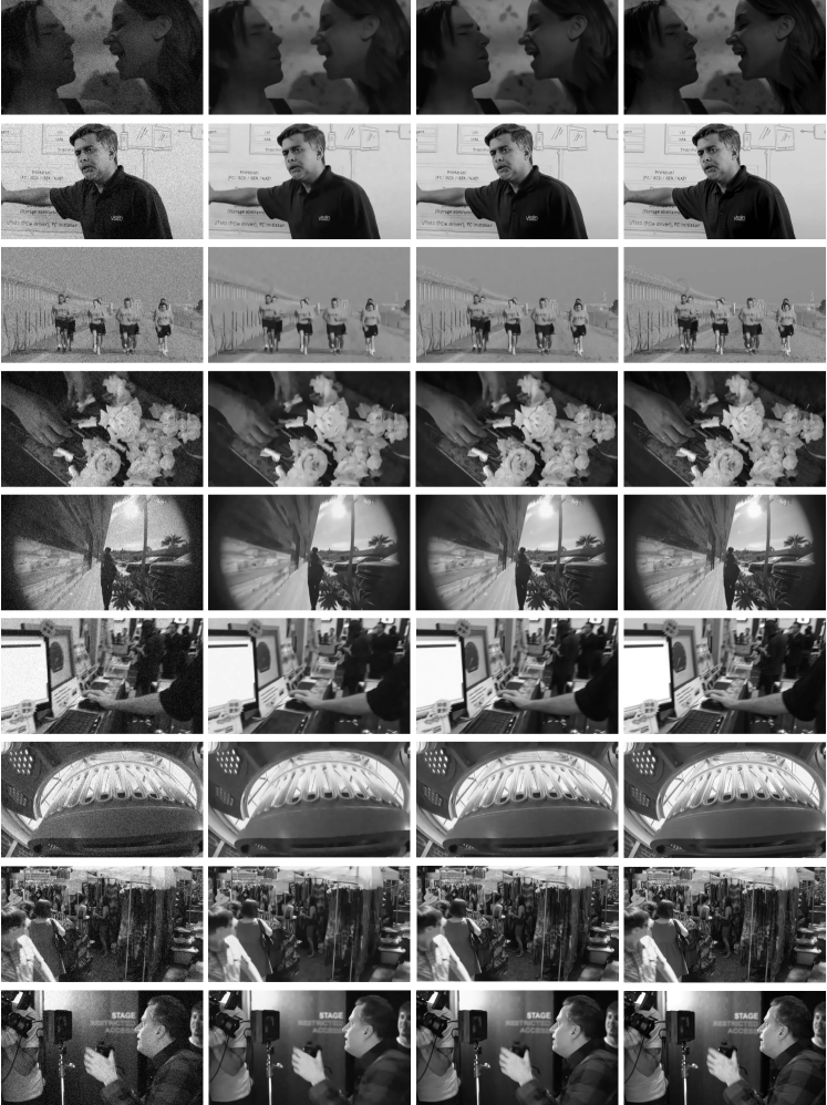
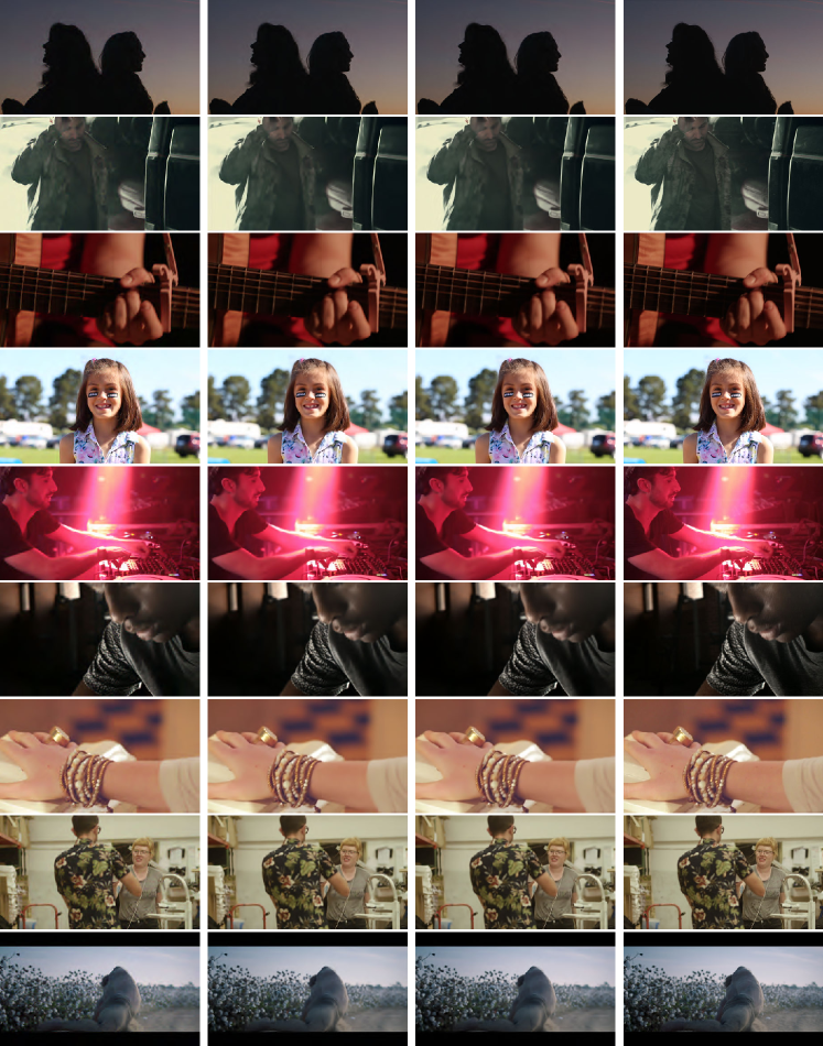
Input

​V-BM4D

TOFlow

Ground Truth

Figure 16: Qualitative results on grayscale video denoising. Samples are randomly selected from the Vimeo denoising benchmark. The differences between different algorithms are clear only when zoomed in.

Input

​V-BM4D

TOFlow

Ground Truth

Figure 17: Qualitative results on video deblocking. Samples are randomly selected from the Vimeo deblocking benchmark. The differences between different algorithms are clear only when zoomed in.

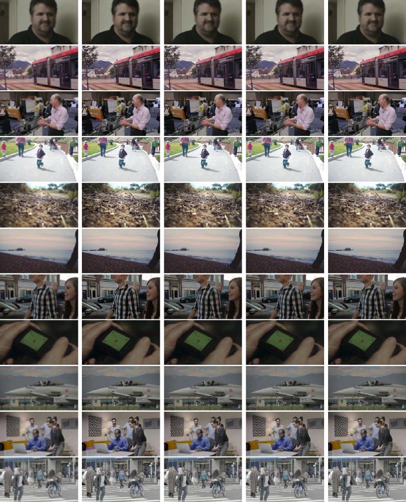
Bicubic

DeepSR

Fixed Flow

TOFlow

Ground Truth

Figure 18: Qualitative results on video super-resolution. Samples are randomly selected from the Vimeo super-resolution benchmark. The differences between different algorithms are clear only when zoomed in. DeepSR was originally trained on 30–50 images, but evaluated on 7 frames in this experiment, so there are some artifacts.

References

- Abu-El-Haija et al (2016) Abu-El-Haija S, Kothari N, Lee J, Natsev P, Toderici G, Varadarajan B, Vijayanarasimhan S (2016) Youtube-8m: A large-scale video classification benchmark. arXiv:160908675
- Ahn et al (2018) Ahn N, Kang B, Sohn KA (2018) Fast, accurate, and, lightweight super-resolution with cascading residual network. In: European Conference on Computer Vision
- Aittala and Durand (2018) Aittala M, Durand F (2018) Burst image deblurring using permutation invariant convolutional neural networks. In: European Conference on Computer Vision, pp 731–747
- Baker et al (2011) Baker S, Scharstein D, Lewis J, Roth S, Black MJ, Szeliski R (2011) A database and evaluation methodology for optical flow. International Journal of Computer Vision 92(1):1–31
- Brox et al (2004) Brox T, Bruhn A, Papenberg N, Weickert J (2004) High accuracy optical flow estimation based on a theory for warping. In: European Conference on Computer Vision
- Brox et al (2009) Brox T, Bregler C, Malik J (2009) Large displacement optical flow. In: IEEE Conference on Computer Vision and Pattern Recognition
- Bulat et al (2018) Bulat A, Yang J, Tzimiropoulos G (2018) To learn image super-resolution, use a gan to learn how to do image degradation first. In: European Conference on Computer Vision
- Butler et al (2012) Butler DJ, Wulff J, Stanley GB, Black MJ (2012) A naturalistic open source movie for optical flow evaluation. In: European Conference on Computer Vision
- Caballero et al (2017) Caballero J, Ledig C, Aitken A, Acosta A, Totz J, Wang Z, Shi W (2017) Real-time video super-resolution with spatio-temporal networks and motion compensation. In: IEEE Conference on Computer Vision and Pattern Recognition
- Fischer et al (2015) Fischer P, Dosovitskiy A, Ilg E, Häusser P, Hazırbaş C, Golkov V, van der Smagt P, Cremers D, Brox T (2015) Flownet: Learning optical flow with convolutional networks. In: IEEE International Conference on Computer Vision
- Ganin et al (2016) Ganin Y, Kononenko D, Sungatullina D, Lempitsky V (2016) Deepwarp: Photorealistic image resynthesis for gaze manipulation. In: European Conference on Computer Vision
- Ghoniem et al (2010) Ghoniem M, Chahir Y, Elmoataz A (2010) Nonlocal video denoising, simplification and inpainting using discrete regularization on graphs. Signal Process 90(8):2445–2455
- Godard et al (2017) Godard C, Matzen K, Uyttendaele M (2017) Deep burst denoising. In: European Conference on Computer Vision
- Horn and Schunck (1981) Horn BK, Schunck BG (1981) Determining optical flow. Artif Intell 17(1-3):185–203
- Huang et al (2015) Huang Y, Wang W, Wang L (2015) Bidirectional recurrent convolutional networks for multi-frame super-resolution. In: Advances in Neural Information Processing Systems
- Jaderberg et al (2015) Jaderberg M, Simonyan K, Zisserman A, et al (2015) Spatial transformer networks. In: Advances in Neural Information Processing Systems
- Jiang et al (2017) Jiang H, Sun D, Jampani V, Yang MH, Learned-Miller E, Kautz J (2017) Super slomo: High quality estimation of multiple intermediate frames for video interpolation. In: IEEE Conference on Computer Vision and Pattern Recognition
- Jiang et al (2018) Jiang X, Le Pendu M, Guillemot C (2018) Depth estimation with occlusion handling from a sparse set of light field views. In: IEEE International Conference on Image Processing
- Jo et al (2018) Jo Y, Oh SW, Kang J, Kim SJ (2018) Deep video super-resolution network using dynamic upsampling filters without explicit motion compensation. In: IEEE Conference on Computer Vision and Pattern Recognition, pp 3224–3232
- Kappeler et al (2016) Kappeler A, Yoo S, Dai Q, Katsaggelos AK (2016) Video super-resolution with convolutional neural networks. IEEE Transactions on Computational Imaging 2(2):109–122
- Kingma and Ba (2015) Kingma DP, Ba J (2015) Adam: A method for stochastic optimization. In: International Conference on Learning Representations
- Li et al (2018) Li M, Xie Q, Zhao Q, Wei W, Gu S, Tao J, Meng D (2018) Video rain streak removal by multiscale convolutional sparse coding. In: IEEE Conference on Computer Vision and Pattern Recognition, pp 6644–6653
- Liao et al (2015) Liao R, Tao X, Li R, Ma Z, Jia J (2015) Video super-resolution via deep draft-ensemble learning. In: IEEE Conference on Computer Vision and Pattern Recognition
- Liu and Freeman (2010) Liu C, Freeman W (2010) A high-quality video denoising algorithm based on reliable motion estimation. In: European Conference on Computer Vision
- Liu and Sun (2011) Liu C, Sun D (2011) A bayesian approach to adaptive video super resolution. In: IEEE Conference on Computer Vision and Pattern Recognition
- Liu and Sun (2014) Liu C, Sun D (2014) On bayesian adaptive video super resolution. IEEE Transactions on Pattern Analysis and Machine intelligence 36(2):346–360
- Liu et al (2017) Liu Z, Yeh R, Tang X, Liu Y, Agarwala A (2017) Video frame synthesis using deep voxel flow. In: IEEE International Conference on Computer Vision
- Lu et al (2018) Lu G, Ouyang W, Xu D, Zhang X, Gao Z, Sun MT (2018) Deep kalman filtering network for video compression artifact reduction. In: European Conference on Computer Vision, pp 568–584
- Ma et al (2015) Ma Z, Liao R, Tao X, Xu L, Jia J, Wu E (2015) Handling motion blur in multi-frame super-resolution. In: IEEE Conference on Computer Vision and Pattern Recognition
- Maggioni et al (2012) Maggioni M, Boracchi G, Foi A, Egiazarian K (2012) Video denoising, deblocking, and enhancement through separable 4-d nonlocal spatiotemporal transforms. IEEE Transactions on Image Processing 21(9):3952–3966
- Makansi et al (2017) Makansi O, Ilg E, Brox T (2017) End-to-end learning of video super-resolution with motion compensation. In: German Conference on Pattern Recognition
- Mathieu et al (2016) Mathieu M, Couprie C, LeCun Y (2016) Deep multi-scale video prediction beyond mean square error. In: International Conference on Learning Representations
- Mémin and Pérez (1998) Mémin E, Pérez P (1998) Dense estimation and object-based segmentation of the optical flow with robust techniques. IEEE Transactions on Image Processing 7(5):703–719
- Mildenhall et al (2018) Mildenhall B, Barron JT, Chen J, Sharlet D, Ng R, Carroll R (2018) Burst denoising with kernel prediction networks. In: IEEE Conference on Computer Vision and Pattern Recognition
- Nasrollahi and Moeslund (2014) Nasrollahi K, Moeslund TB (2014) Super-resolution: a comprehensive survey. Machine Vision and Applications 25(6):1423–1468
- Niklaus and Liu (2018) Niklaus S, Liu F (2018) Context-aware synthesis for video frame interpolation. In: IEEE Conference on Computer Vision and Pattern Recognition
- Niklaus et al (2017a) Niklaus S, Mai L, Liu F (2017a) Video frame interpolation via adaptive convolution. In: IEEE Conference on Computer Vision and Pattern Recognition
- Niklaus et al (2017b) Niklaus S, Mai L, Liu F (2017b) Video frame interpolation via adaptive separable convolution. In: IEEE International Conference on Computer Vision
- Oliva and Torralba (2001) Oliva A, Torralba A (2001) Modeling the shape of the scene: A holistic representation of the spatial envelope. International Journal of Computer Vision 42(3):145–175
- Ranjan and Black (2017) Ranjan A, Black MJ (2017) Optical flow estimation using a spatial pyramid network. In: IEEE Conference on Computer Vision and Pattern Recognition
- Revaud et al (2015) Revaud J, Weinzaepfel P, Harchaoui Z, Schmid C (2015) Epicflow: Edge-preserving interpolation of correspondences for optical flow. In: IEEE Conference on Computer Vision and Pattern Recognition
- Sajjadi et al (2018) Sajjadi MS, Vemulapalli R, Brown M (2018) Frame-recurrent video super-resolution. In: IEEE Conference on Computer Vision and Pattern Recognition, pp 6626–6634
- Tao et al (2017) Tao X, Gao H, Liao R, Wang J, Jia J (2017) Detail-revealing deep video super-resolution. In: IEEE International Conference on Computer Vision
- Varghese and Wang (2010) Varghese G, Wang Z (2010) Video denoising based on a spatiotemporal gaussian scale mixture model. IEEE Transactions on Circuits and Systems for Video Technology 20(7):1032–1040
- Wang et al (2017) Wang TC, Zhu JY, Kalantari NK, Efros AA, Ramamoorthi R (2017) Light field video capture using a learning-based hybrid imaging system. In: SIGGRAPH
- Wedel et al (2009) Wedel A, Cremers D, Pock T, Bischof H (2009) Structure-and motion-adaptive regularization for high accuracy optic flow. In: IEEE Conference on Computer Vision and Pattern Recognition
- Wen et al (2017) Wen B, Li Y, Pfister L, Bresler Y (2017) Joint adaptive sparsity and low-rankness on the fly: an online tensor reconstruction scheme for video denoising. In: IEEE International Conference on Computer Vision (ICCV)
- Werlberger et al (2011) Werlberger M, Pock T, Unger M, Bischof H (2011) Optical flow guided tv-l1 video interpolation and restoration. In: International Conference on Energy Minimization Methods in Computer Vision and Pattern Recognition
- Xu et al (2017) Xu J, Ranftl R, Koltun V (2017) Accurate optical flow via direct cost volume processing. In: IEEE Conference on Computer Vision and Pattern Recognition
- Xu et al (2015) Xu S, Zhang F, He X, Shen X, Zhang X (2015) Pm-pm: Patchmatch with potts model for object segmentation and stereo matching. IEEE Transactions on Image Processing 24(7):2182–2196
- Yang et al (2018) Yang R, Xu M, Wang Z, Li T (2018) Multi-frame quality enhancement for compressed video. In: IEEE Conference on Computer Vision and Pattern Recognition, pp 6664–6673
- Yu et al (2016) Yu JJ, Harley AW, Derpanis KG (2016) Back to basics: Unsupervised learning of optical flow via brightness constancy and motion smoothness. In: European Conference on Computer Vision Workshops
- Yu et al (2013) Yu Z, Li H, Wang Z, Hu Z, Chen CW (2013) Multi-level video frame interpolation: Exploiting the interaction among different levels. IEEE Transactions on Circuits and Systems for Video Technology 23(7):1235–1248
- Zhou et al (2016) Zhou T, Tulsiani S, Sun W, Malik J, Efros AA (2016) View synthesis by appearance flow. In: European Conference on Computer Vision
- Zhu et al (2017) Zhu X, Wang Y, Dai J, Yuan L, Wei Y (2017) Flow-guided feature aggregation for video object detection. In: IEEE International Conference on Computer Vision
- Zitnick et al (2004) Zitnick CL, Kang SB, Uyttendaele M, Winder S, Szeliski R (2004) High-quality video view interpolation using a layered representation. ACM Transactions on Graphics 23(3):600–608