Convolutional Image Captioning

Abstract

Image captioning is an important but challenging task, applicable to virtual assistants, editing tools, image indexing, and support of the disabled. Its challenges are due to the variability and ambiguity of possible image descriptions. In recent years significant progress has been made in image captioning, using Recurrent Neural Networks powered by long-short-term-memory (LSTM) units. Despite mitigating the vanishing gradient problem, and despite their compelling ability to memorize dependencies, LSTM units are complex and inherently sequential across time. To address this issue, recent work has shown benefits of convolutional networks for machine translation and conditional image generation [9, 34, 35]. Inspired by their success, in this paper, we develop a convolutional image captioning technique. We demonstrate its efficacy on the challenging MSCOCO dataset and demonstrate performance on par with the baseline, while having a faster training time per number of parameters. We also perform a detailed analysis, providing compelling reasons in favor of convolutional language generation approaches.

1 Introduction

Image captioning, i.e., describing the content observed in an image, has received a significant amount of attention in recent years. It is applicable in various scenarios, e.g., recommendation in editing applications, usage in virtual assistants, for image indexing, and support of the disabled. It is also a basic ingredient for more complex operations such as storytelling [13] and visual summarization [37].

In recent years, with the availability of larger datasets, deep neural network (DNN) based methods have been shown to achieve impressive results on image captioning tasks [16, 38]. These techniques are largely based on recurrent neural nets (RNNs), often powered by a Long-Short-Term-Memory (LSTM) [11] component which mitigates the issue of vanishing or exploding gradients [25]. Figure 1 shows examples of captions generated by an LSTM-based network.

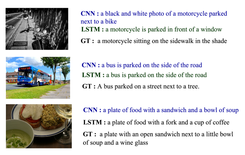
Figure 1: Examples of captions generated by a standard LSTM-based network, our convolutional network (CNN) and ground-truth (GT) captions by a human annotator.

LSTM nets have been considered as the de-facto standard for vision-language tasks of image captioning [5, 16, 38, 39], visual question answering [2, 30], question generation [14, 21], situation recognition [19], and visual dialog [7], due to their compelling ability to memorize long-term dependencies through a memory cell. However, the complex addressing and overwriting mechanism combined with inherently sequential processing, and significant storage required due to back-propagation through time (BPTT), poses challenges during training. Also, in contrast to CNNs, that are non-sequential, LSTMs often require more careful engineering, when considering a novel task. Previously, CNNs have not matched up to the LSTM performance on vision-language tasks.

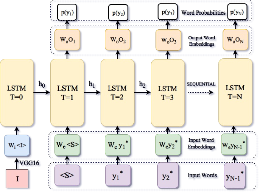
Figure 2: A sequential RNN powered by an LSTM cell. At each time step output is conditioned on the previously generated word, the image is fed at the start only.

Inspired by the recent successes of convolutional architectures on other sequence-to-sequence tasks – conditional image generation [34], machine translation [9, 35] – we study convolutional architectures for the task of image captioning. To the best of our knowledge, ours is the first convolutional network for image captioning that compares favorably to LSTM-based methods. On the MSCOCO dataset we match performance of the LSTM with a .952 CIDEr score and get a better BLEU-4 score of .316 (see Table 2).

Our key contributions are: a) A convolutional (CNN-based) image captioning method that shows comparable performance to an LSTM based method on standard metrics (Section 6.2, Table 1 and Table 2); b) Improved performance with a CNN model that uses attention mechanism to leverage spatial image features. With attention, we outperform the current attention baseline and qualitatively demonstrate that our method finds salient objects in the image. (Figure 6, Table 2); c) We analyze the characteristics of CNN and LSTM nets and provide useful insights such as – CNNs produce more entropy (useful for diverse predictions), better classification accuracy, and do not suffer from vanishing gradients (Section 6 and Figure 7, 8 and 9). We evaluate our architecture on the challenging MSCOCO [18] dataset, and compare it to an LSTM [16] and an LSTM+Attention baseline [39].

The paper is organized as follows: Section 2 describes our notation, Section 3 briefly reviews the RNN/LSTM based approach, Section 4 describes our convolutional method and Section 5 gives the details of our CNN architecture, Section 6 contains our results and Section 7 discusses previous work on image captioning.

2 Problem Setup and Notation

For image captioning, we are given an input image $I$ and we are required to generate a sequence of words $y=(y_{1},\ldots,y_{N})$. The possible words $y_{i}\in{\mathcal{Y}}$ at time-step $i$ are subsumed in a discrete set ${\mathcal{Y}}$ of options. The number of possible options $|{\mathcal{Y}}|$ easily reaches several thousands. This set of options ${\mathcal{Y}}$ often contains special tokens that denote a start token ($<$S$>$), an end of sentence token ($<$E$>$), and an unknown token ($<$UNK$>$) which refers to all words not in ${\mathcal{Y}}$.

Given a training set ${\mathcal{D}}=\{(I,y^{\ast})\}$ which contains pairs $(I,y^{\ast})$ of input image $I$ and corresponding ground-truth caption $y^{\ast}=(y^{\ast}_{1},\ldots,y^{\ast}_{N})$, consisting of words $y^{\ast}_{i}\in{\mathcal{Y}}$, $i\in\{1,\ldots,N\}$, we maximize w.r.t. parameters $w$, a probabilistic model $p_{w}(y_{1},\ldots,y_{N}|I)$.

A variety of probabilistic models have been considered (Section 7), from hidden Markov models [40] to recurrent neural networks. First, we briefly review the inference and learning of RNN-based approaches (Section 3) and then delve into our convolutional approach (Section 4).

3 RNN Approach

An illustration of a classical RNN architecture for image captioning is provided in Figure 2. It consists of three major components, all of which contain trainable parameters: the input word embeddings, the sequential LSTM units containing the memory cell, and the output word embeddings.

Inference. RNNs sequentially predict one word at a time, from $y_{1}$ up to $y_{N}$. At every time-step $i$, a conditional probability distribution $p_{i,w}(y_{i}|I)$, which depends on parameters $w$, is predicted (see top of Figure 2). During inference, we typically choose the word $y_{i}$ with the highest probability $p_{i,w}(y_{i}|I)$. The sentence terminates once the end of sentence token is chosen, or after a maximum of $N$ steps.

For modeling $p_{i,w}(y_{i}|I)$, in the spirit of auto-regressive models, the dependence of word $y_{i}$ on its ancestors $y_{<i}$ is implicitly captured by a hidden representation $h_{i}$ (see arrows in Figure 2). Formally, the probability is computed via

$$p_{i,w}(y_{i}|h_{i},I)=g_{w}(y_{i},h_{i},I),$$ (1)

where $g_{w}$ can be any differentiable function/deep net. This function may depend directly on the image $I$. However, classical image captioning techniques usually encode the image into the hidden representation $h_{0}$ (Figure 2).

Importantly, RNNs just like other auto-regressive models are described by a recurrence relation which governs computation of the hidden state $h_{i}$ based on its values at the previous time instant, $h_{i-1}$, as well as the word $y_{i-1}$, predicted at the previous time step:

$$h_{i}=f_{w}(h_{i-1},y_{i-1},I).$$ (2)

Again, $f_{w}$ can be any differentiable function. For image captioning, long-short-term-memory (LSTM) [11] nets and variants thereof based on gated recurrent units (GRU) [6], or forward-backward LSTM nets are used here.

The recurrent function given in Eq. (2) generally doesn’t operate directly on one-hot input vectors $y_{i}$. Instead, input words are encoded into a vectorial representation via an embedding layer (input word embeddings in Figure 2). Note that the functions $g_{w}$ and $f_{w}$ are identical across time.

Learning. Following classical supervised learning, it is common to find the parameters $w$ of the word embeddings and the LSTM unit by minimizing the negative log-likelihood of the training data ${\mathcal{D}}$, i.e., we optimize:

$$\min_{w}-\sum_{(I,y^{\ast})\in{\mathcal{D}}}\sum_{i=1}^{N}\ln p_{i,w}(y^{\ast}_{i}|h_{i},I).$$ (3)

To compute the gradient of the objective given in Eq. (3), back-propagation through time (BPTT) is the de-facto standard these days. BPTT is necessary due to the recurrence relationship encoded in $f_{w}$ (Eq. (2)), which is unrolled as illustrated in Figure 2. The gradients of the function $f_{w}$ at time $i$ depend on the gradients obtained in successive time-steps.

To avoid more complicated gradient flows through the recurrence relationship, during training, it is common to use

$$h_{i}=f_{w}(h_{i-1},y^{\ast}_{i-1},I),$$ (4)

rather than the form provided in Eq. (2). I.e., during training, when computing the latent representation $h_{i}$, we use the ground-truth symbol $y^{\ast}_{i-1}$ rather than the prediction $y_{i-1}$. This is termed as teacher forcing. While this simplifies the gradient flow, it obviously causes the input statistics to differ between train and test. This issue has been subject to recent work [4, 10].

Although highly successful, RNN-based techniques suffer from some drawbacks. First, the training process is inherently sequential for a particular image-caption pair. This results from unrolling the recurrent relation in time. Hence, the output at time-step $i$ has a true dependency on the output at $i-1$. Secondly, as we will show in our results for image captioning, RNNs tend to produce lower classification accuracy (Figure 7), and, despite LSTM units, they still suffer to some degree from vanishing gradients (Figure 9).

Next, we describe an alternative convolutional approach to image captioning which attempts to overcome some of these challenges.

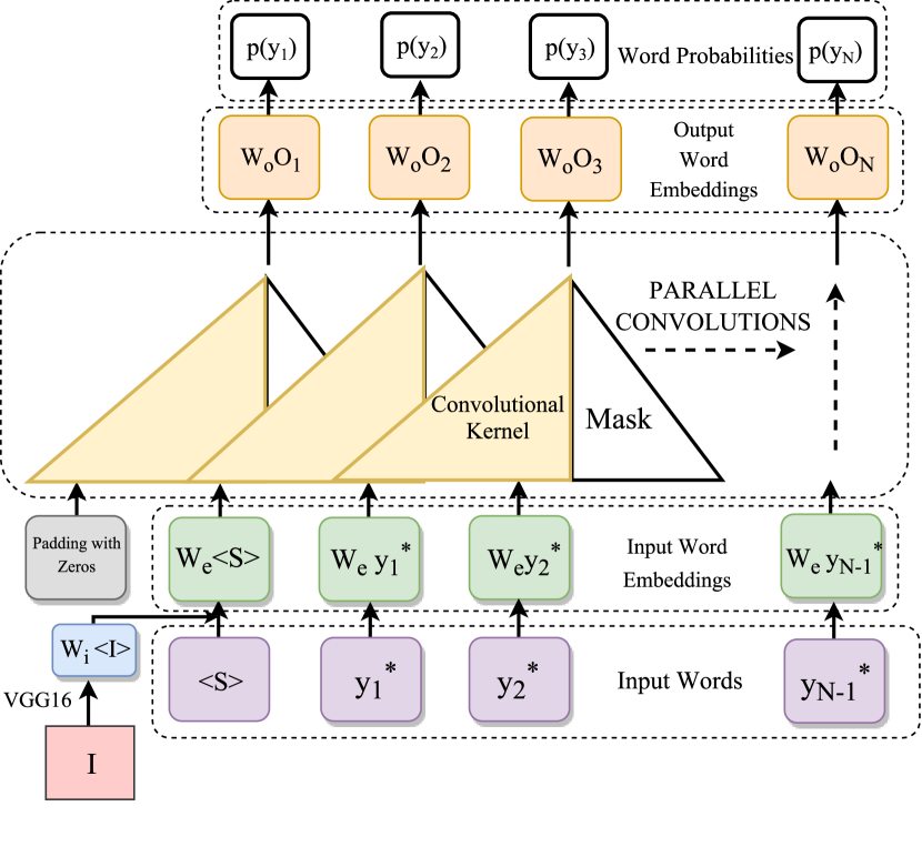
Figure 3: Our convolutional model for image captioning. We use a feed forward network with masked convolutions. Unlike RNNs, our model operates over all words in parallel.

4 Convolutional Approach

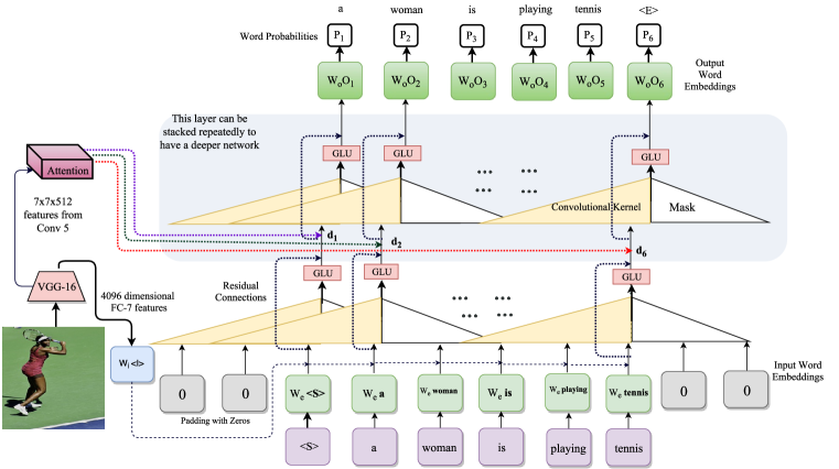
Figure 4: Our convolutional architecture for image captioning. Our architecture has four components: (i) Input embedding layer, (ii) Image embedding, (iii) Convolutional module and (iii) Output embedding layer. Details of these components can be found in Section 5.

Our model is based on the convolutional machine translation model used in [9]. Figure 3 provides an overview of our feed-forward convolutional (or CNN-based) approach for image captioning. As the figure illustrates, our technique contains three main components similar to the RNN technique. The first and the last components are word embeddings in both cases. However, while the center component contains LSTM or GRU units in the RNN case, masked convolutions are employed in our CNN-based approach. This component, unlike the RNN, is feed-forward without any recurrent function. We briefly review inference and learning of our model. The problem setup and notation follows Section 2.

Inference. In contrast to the RNN formulation, where the probabilistic model is unrolled in time via the recurrence relation given in Eq. (4), we use a simple feed-forward deep net, $f_{w}$, for modeling $p_{i,w}(y_{i}|I)$. Prediction of a word $y_{i}$ relies on past words $y_{<i}$ or their representations:

$$p_{i,w}(y_{i}|y_{<i},I)=f_{w}(y_{i},y_{<i},I).$$ (5)

To disallow convolution operations from using information of future word tokens, we use masked convolutional layers that operate only on ‘past’ data. This is similar to [9, 34].

Inference can now be performed sequentially, one word at a time. Hence, inference begins with the start token $<$S$>$ and employs a feed-forward pass to generate $p_{1,w}(y_{1}|\emptyset,I)$. Afterwards, $y_{1}\sim p_{1,w}(y_{1}|\emptyset,I)$ is sampled. Note that it is possible to retrieve the maximizing argument or to perform beam search. After sampling, $y_{1}$ is fed back into the feed-forward network to generate subsequent words $y_{2}$, etc. Inference continues until the end token is predicted, or until we reach a fixed upper bound of $N$ steps.

Learning. Similar to RNN training, we use ground-truth $y^{\ast}_{<i}$ for past words, instead of using the most recently generated ones. For prediction of word probability $p_{i,w}(y_{i}|y_{<i}^{\ast},I)$, the considered feed-forward network is $f_{w}(y_{i},y^{\ast}_{<i},I)$ and we optimize for parameters $w$ using a likelihood similar to Eq. (3).

Since there are no recurrent connections and all ground-truth words are available at any given time-step $i$, our CNN based model can be trained in parallel for all words. In Section 5, we provide details about the convolutional architecture used in our experiments.

5 Architecture

The detailed architecture for our convolutional image captioning is illustrated in Figure 4. In this figure, we show a training iteration with input (ground-truth) words {$y^{\ast}_{1},\ldots,y^{\ast}_{5}$} = $\{$ a, woman, is, playing, tennis $\}$. Additionally, we add the start token $<$S$>$ at the beginning and also, the end of sentence token $<$E$>$.

These words are processed as follows: (1) they pass through an input embedding layer; (2) they are combined with the image embedding; (3) they are processed by the CNN module; and (4) the output embedding (or classification) layer produces output probability distributions (see $\{p_{1},\ldots,p_{6}\}$ at top of Figure 4). Each of the four aforementioned steps is discussed below.

Input Embedding. For consistency with RNN/LSTM baseline, we train (from scratch) an embedding layer over one-hot encoded input words. We use $|{\mathcal{Y}}|=9221$ and we embed the input words to $512$-dimensional vectors, same as the baseline. This embedding is concatenated to the image embedding (discussed next) and provided as input to the feed-forward CNN module.

Image Embedding. Image features for image $I$, are obtained from the fc7 layer of the VGG16 network [31]. The VGG16 is pre-trained on the ImageNet dataset [28]. We apply dropout, ReLU on the fc7 and use a linear layer to obtain a $512$-dimensional embedding. This is consistent with the image features used in the baseline LSTM method [16].

Method	MSCOCO Val Set								MSCOCO Test Set
	B1	B2	B3	B4	M	R	C	S	B1	B2	B3	B4	M	R	C	S
Baselines:
LSTM [16]	.710	.535	.389	.281	.244	.521	.899	.169	.713	.541	.404	.303	.247	.525	.912	.172
LSTM + Attn (Soft) [39]	-	-	-	-	-	-	-	-	.707	.492	.344	.243	.239	-	-	-
LSTM + Attn (Hard) [39]	-	-	-	-	-	-	-	-	.718	.504	.357	.250	.230	-	-	-
Our CNN:
CNN	.693	.518	.374	.268	.238	.511	.855	.167	.695	.521	.380	.276	.241	.514	.881	.171
CNN + Weight Norm.	.702	.528	.384	.279	.242	.517	.881	.169	.699	.525	.382	.276	.241	.516	.878	.170
CNN +WN +Dropout	.707	.532	.386	.278	.242	.517	.883	.171	.704	.532	.389	.283	.243	.520	.904	.173
CNN +WN +Dropout +Residual	.706	.532	.389	.284	.244	.519	.899	.173	.704	.532	.389	.284	.244	.520	.906	.175
CNN +WN +Drop. +Res. +Attn	.710	.537	.391	.281	.241	.519	.890	.171	.711	.538	.394	.287	.244	.522	.912	.175

Table 1: Comparison of different methods on standard evaluation metrics: BLEU-1 (B1), BLEU-2 (B2), BLEU-3 (B3), BLEU-4 (B4), METEOR (M), ROUGE (R), CIDEr (C) and SPICE (S). Our CNN with attention (attn) achieves comparable performance (equal CIDEr scores on MSCOCO test set) to [16] and outperforms LSTM+Attention baseline of [39]. We experiment with various configurations of our CNN. We start with a CNN comprising masked convolutions and fully connected layers only. Then, we add weight normalization, dropout, residual connections and attention incrementally and show that performance improves with every addition. Here, for our CNN and [16] we use the model that obtains the best CIDEr scores on val-set and report its scores for the test set. We evaluate CIDEr scores after every training epoch for val-set. Note, the val set is not used for any hyper-parameter tuning other than choosing the best model for test set. For [39], we report all the available metrics for soft/hard attention from their paper (missing numbers are marked by -).

Method	Beam Size=2								Beam Size=3								Beam Size=4
	B1	B2	B3	B4	M	R	C	S	B1	B2	B3	B4	M	R	C	S	B1	B2	B3	B4	M	R	C	S
LSTM [16]	.715	.545	.407	.304	.248	.526	.940	.178	.715	.544	.409	.310	.249	.528	.946	.178	.714	.543	.410	.311	.250	.529	.951	.179
CNN	.712	.541	.404	.303	.248	.527	.937	.178	.709	.538	.403	.303	.247	.525	.929	.176	.706	.533	.400	.302	.247	.522	.925	.175
CNN+Attn	.718	.549	.411	.306	.248	.528	.942	.177	.722	.553	.418	.316	.250	.531	.952	.179	.718	.550	.415	.314	.249	.528	.951	.179

Table 2: Comparison of different methods (metrics same as Table 1) with beam search on the output word probabilities. Our results show that with beam size$=3$ our CNN outperforms LSTM [16] on all metrics. Note, compared to Table 1, the performance improves with beam search. We use the MS COCO test split for this experiment. For beam search, we pick one caption with maximum log probability (sum of log probability of words) from the top-$k$ beams and report the above metrics for it. Beam $=1$ is same as the test set results reported in Table 1.

CNN Module. The CNN module operates on the combined input and image embedding vector. It performs three layers of masked convolutions, keeping the feature dimensions after convolution to $512$. Consistent with [9, 34], we use gated linear unit (or GLU) activations for our conv layers. However, we did not observe a significant change in performance when using the standard ReLU activation. We experiment with weight normalization, residual connections and dropout in these layers and show that they help improve performance (Table 1). Our masked convolutions have a receptive field of 5 words in the past. We set $N$ (steps or max-sentence length) to $15$ for both CNN/RNN. The output of the CNN module after three layers is a $512$-dimensional vector for each word.

Classification Layer. We use a linear layer to encode the $512$-dimensional vectors obtained from the CNN module into a $256$-dimensional representation per word. Then, we upsample this vector to a $|{\mathcal{Y}}|$-dimensional activation via a fully connected layer, and pass it through a softmax to obtain the output word probabilities $p_{i,w}(y_{i}|I)$.

Training. We use a cross-entropy loss on the probabilities $p_{i,w}(y_{i}|y_{<i},I)$ to train the CNN module and the embedding layers. Consistent with [16], we start to fine-tune VGG16 along with our network after 8 training epochs. We optimize with RMSProp using an initial learning rate of $5e^{-5}$ and decay the learning rate by a factor of $.1$ after every 15 epochs. All methods were trained for 30 epochs and we evaluate the metrics (given in Section 6.2) on the validation set to pick the best model for each method.

5.1 Attention

In addition to the aforementioned CNN architecture, we also experiment with an attention mechanism, since attention benefited [9, 35]. We form an attended image vector of dimension $512$ and add it to the word embedding at every layer (shown with red, green and blue arrows in Figure 4). We compute separate attention parameters and a separate attended vector for every word. To obtain this attended vector we predict $7\times 7$ attention parameters, over the VGG16 max-pooled conv-5 features of dimensions $7\times 7\times 512$ [31]. We use attention on all three masked convolution layers in our CNN module. We continue to use the fc7 image embedding discussed above.

To discuss attention more formally, let $d_{j}$ denote the embedding of word $j$ in the conv module (i.e., its activations after GLU shown in Figure 4), let $W$ refer to a linear layer applied to $d_{j}$, let $c_{i}$ denote a $512$-dimensional spatial conv-5 feature at location $i$ (in $7\times 7$ feature map) and let $a_{ij}$ indicate the attention parameters. With this notation at hand, the attention parameter $a_{ij}$ is computed via

$$a_{ij}=\frac{\exp(W(d_{j})^{T}c_{i})}{\sum\limits_{i}\exp(W(d_{j})^{T}c_{i})},$$ (6)

and the attended image vector for word $j$ is obtained from $\sum\limits_{i}a_{ij}c_{i}$.

Note that [39] uses the LSTM hidden state to compute the attention parameters. Instead, we compute attention parameters using the conv-layer activations. This form of attention mechanism was first proposed in [3].

	c5 (Beam = 1)							c40 (Beam = 1)
	B1	B2	B3	B4	M	R	C	B1	B2	B3	B4	M	R	C
LSTM	.704	.528	.384	.278	.241	.517	.876	.880	.778	.656	.537	.321	.655	.898
CNN+Attn	.708	.534	.389	.280	.241	.517	.872	.883	.786	.667	.545	.321	.657	.893
	c5 (Beam = 3)							c40 (Beam = 3)
	B1	B2	B3	B4	M	R	C	B1	B2	B3	B4	M	R	C
LSTM	.710	.537	.399	.299	.246	.523	.904	.889	.794	.681	.570	.334	.671	.912
CNN+Attn	.715	.545	.408	.304	.246	.525	.910	.896	.805	.694	.582	.333	.673	.914

Table 3: Above, we show that CNN outperforms LSTM on BLEU metrics and gives comparable scores to LSTM on other metrics for test split on MSCOCO evaluation server. Here, we submitted our results to the MSCOCO evaluation server to evaluate on the hidden test split. Note, this test split of $40,775$ images is different from the $5000$ images test split used in Tables 1 and 2. We compare our CNN+Attn method to the LSTM baseline on standard evaluation metrics: BLEU-1 (B1), BLEU-2 (B2), BLEU-3 (B3), BLEU-4 (B4), METEOR (M), ROUGE (R) and CIDEr (C). The $c5$ scores above are computed with $5$ reference captions per test image and $c40$ scores are computed with $40$ reference captions. We show comparison results for beam size 1 and beam size 3 for both the methods.

6 Results and Analysis

LSTM: a man and a woman in a suit and tie CNN: a black and white photo of a man and woman in a suit GT: A man sitting next to a woman while wearing a suit.	LSTM: a man is walking down a path in the woods CNN: a truck is parked in the dirt near a tree GT: a truck is parked at a campground with snow on it	LSTM: a cat is laying down on a bed CNN: a polar bear is drinking water from a white bowl GT: A white polar bear laying on top of a pool of water	LSTM: a bear is standing on a rock in a zoo CNN: two bears are walking on a rock in the zoo GT: two bears touching noses standing on rocks	LSTM: a box of donuts with a variety of toppings CNN: a box of doughnuts with sprinkles and a sign GT:A bunch of doughnuts with sprinkles on them
LSTM: a dog is standing in the grass near a tree CNN: a dog is standing in the grass with a frisbee in its mouth GT: large dog retrieving the frisbee for his owner	LSTM: a parking meter with a sign on it CNN: a doll is sitting next to a parking meter GT: A doll with articulated joints stares from her perch between two parking meters.	LSTM: a boat is docked in the water near a dock CNN: a boat is docked in the water near a mountain GT: A white boat floating on a lake under mountains	LSTM: a cat is standing on top of a refrigerator CNN: a cat is standing in a kitchen looking at the camera GT: A cat in a kitchen on top of a refrigerator	LSTM: a dog and a dog in a field CNN: two cows are standing in a field of grass GT: A dog and a horse standing near each other

Figure 5: Captions generated by our CNN are compared to the LSTM and ground-truth caption. In the examples above our CNN can describe things like black and white photo, polar bear/white bowl, number of bears, sign in the donut image which LSTM fails to do. The last two images (bottom right) show failure cases for CNN. Typically we observe that CNN and LSTM captions are of similar quality. We use our CNN+Attn method (Section 5.1) and the MSCOCO test split for these results.

In this section, we demonstrate the following results:

• Our convolutional (or CNN) approach performs on par with LSTM (or RNN) based approaches on image captioning metrics (Table 1). Our performance improves with beam search (Table 2).

• Adding attention to our CNN gives improvements on metrics and we outperform the LSTM+Attn baseline [39] (Table 1). Figure 6 shows that with attention we identify salient objects for the given image.

• We analyze the CNN and RNN approaches and show that CNN produces (1) more entropy in the output probability distribution, (2) gives better word prediction accuracy (Figure 7), and (3) does not suffer as much from vanishing gradients (Figure 9).

• In Table 4, we show that a CNN with $1.5\times$ more parameters can be trained in comparable time. This is because we avoid the sequential processing of RNNs.

The details of our experimental setup and these results are discussed below. PyTorch implementation of our convolutional image captioning is available on github.

CNN: a baby holding a toothbrush in his hand GT: A child holds a toothbrush in their hand.	a	baby	holding	a	toothbrush	in	… hand
CNN: a plate of food with broccoli and rice GT: A BBQ steak on a plate next to mashed potatoes and mixed vegetables.	a	plate	of	food	with	broccoli	… rice
CNN: a man sitting on a bench overlooking the ocean GT: A man sitting on top of a bench near the ocean	a	man	sitting	on	a	bench	… ocean

Figure 6: We overlay the attention parameters on the image. These results show that we focus on salient objects such as broccoli, bench, toothbrush in the image when predicting these words. Also, the attention is spread out/uniform when predicting words such as a, of and on which are unrelated to image content.

6.1 Dataset and Baselines

We conducted experiments on the MS COCO dataset [18]. Our train/val/test splits follow [16, 39]. We use 113287 training images, 5000 images for validation, and 5000 for testing. Henceforth, we will refer to our approach as CNN, and our approach with the attention (Section 5.1) as CNN+Attn. We use the following naming convention for our baselines: [16] is denoted by LSTM and [39] is referred to as LSTM+Attn.

6.2 Comparison on Image Captioning Metrics

We consider multiple conventional evaluation metrics, BLEU-1, BLEU-2, BLEU-3, BLEU-4 [24], METEOR [8], ROUGE [17], CIDEr [36] and SPICE [1]. See Table 1 for the performance on all these metrics for our val/test splits. Note that we obtain comparable CIDEr scores and better SPICE scores than LSTM on test set with our CNN+Attn method. Our BLEU, METEOR, ROUGE scores are less than the LSTM ones, but the margin is very small. Our CNN+Attn method outperforms the LSTM+Attn baseline on the test set for all metrics reported in [39]. For Table 1, we form the caption by choosing the word with maximum probability at each step. The metrics are reported for this one caption formed by choosing maximum probability word at every step.

Instead of sampling the maximum probability words, we also perform beam search with different beam sizes. We perform beam search for both LSTM and our CNN methods. With beam search, we pick the maximum probability caption (sum of log word probability in the beam). The results reported in Table 2 demonstrate that with beam size of $3$ we achieve better BLEU, ROUGE, CIDEr scores than LSTM and equal METEOR and SPICE scores.

In Table 3, we show the results obtained on the MSCOCO evaluation server. These results are computed over a test set of $40,775$ images for which ground-truth is not publicly available. We demonstrate that our method does better on all BLEU metrics, especially with beam size 3, we perform better than the LSTM based method.

6.3 Qualitative Comparison

See Figure 5 for a qualitative comparison of captions generated by CNN and LSTM. In Figure 6, we overlay the attention parameters on the image for each word prediction. Note that our attention parameters are $7\times 7$ as described in Section 5.1 and therefore the image is divided in a $7\times 7$ grid. These results show that our attention focuses on salient objects such as man, broccoli, ocean, bench, etc., when predicting these respective words. Our results also show that the attention is uniform when predicting words such as a, of, on, etc., which are unrelated to the image content.

6.4 Analysis of CNN and RNN

In Table 4 we report the number of trainable parameters and the training time per epoch. CNNs with $1.5$ times more parameters can be trained in comparable time.

Table 1, 2 and 3 show that we obtain comparable performance from both CNN and RNN/LSTM-based methods. Encouraged by this result, we analyze the characteristics of these two methods. For fair comparison, we use our CNN without attention, since the RNN method does not use spatial image features. First, we compare the negative log- likelihoods (or cross-entropy loss) on a subset of train and the entire val set (see Figure 7 (a)). We find that the loss is higher for CNN than RNN, this is because CNNs are being penalized for producing less-peaky word probability distributions. To evaluate this further, we plot the entropy of the output probability distribution (Figure 7 (b)) and the classification accuracy, i.e., the number of times the maximum probability word is the ground truth (Figure 7 (c)). These plots show that RNNs are good at producing low entropy and therefore peaky word probability distributions at the output, while CNNs produce less peaky distributions (and high entropy). Less peaky distributions are not necessarily bad, particularly for a problem like image captioning, where multiple word predictions are possible. Despite, less peaky distributions, Figure 7(c) shows that the maximum probability word is correct more often on the train set and it is within approx. $1\%$ accuracy on the val set. Note, cross-entropy loss is a proxy for the classification accuracy and we show that CNNs have higher cross entropy loss, but their classification accuracy is good. Less peaky posterior distributions provided by a CNN may be indicative of CNNs being more capable of predicting diverse captions.

In Figure 8, we plot the unique words predicted at every word position or time-step. The plot is for word positions $1$ to $13$. This plot shows that for the CNN we have higher unique words for more word positions than LSTM. This supports our analysis that CNNs have less peaky (or one-hot) posteriors and therefore can produce more diversity. For these diversity experiments, we perform a beam search with beam size 10 and use all the top 10 beams.

Since RNNs/LSTMs are known to suffer from vanishing gradient problems, in Figure 9, we plot the gradient norm at the output embedding/classification layer and the gradient norm at the input embedding layer. The values are averaged over 1 training epoch. These plots show that the gradients in RNN/LSTM diminishes more than the ones in CNNs. Hence RNN/LSTM nets are more likely to suffer from vanishing gradients, which stalls learning. If learning is stalled, for larger datasets than the ones we currently use for image captioning, the performance of RNN and CNN may differ significantly.

Method	# Parameters	Train time per epoch
LSTM [16]	13M	1529s
Our CNN	19M	1585s
Our CNN+Attn	20M	1620s

Table 4: Comparison of train time (in seconds) for LSTM and CNN. We train a CNN faster per parameter than the LSTM. This is because CNN is not sequential like the LSTM. We use PyTorch implementation of [16] and our CNN-based method for fair comparison. The timings are obtained on Nvidia Titan X GPU.

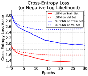
(a) CNN gives higher cross-entropy loss on train/val set of MSCOCO compared to LSTM. But, as we show in (c), our CNN obtains better $\%$ word accuracy than LSTM. Therefore, it still assigns max. probability to correct word. The CNN loss is high because our output probability distributions have more entropy than LSTM.

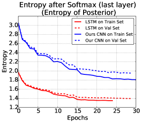
(b) The entropy of the softmax layer (or posterior probability distribution) of our CNN is higher than the LSTM. For ambiguous problems such as image captioning, it is desirable to have a less peaky (multi-modal) posterior (like ours) capable of producing multiple captions, rather than a peaky one (like LSTM).

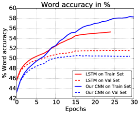
(c) Even though the CNN training loss is higher than LSTM, its word prediction accuracy is better than LSTM on train set. On val set, the difference in accuracy between LSTM and CNN is small (only $\sim 1\%$).

Figure 7: In the figures above we plot (a) Cross-entropy loss, (b) Entropy of the softmax layer, (c) Word accuracy on train/val set. Blue line denotes our method and red denotes the LSTM based method [16]. In (a), (b) and (c) solid/dotted lines denote train/val set of MSCOCO respectively. For these plots, at the end of every epoch we randomly sample $10$k images from train set and use the entire val set.

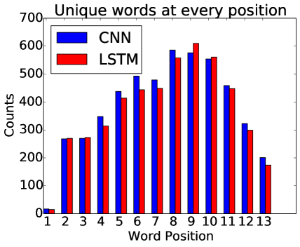
Figure 8: We perform beam search of beam size 10 with our best performing LSTM and CNN models. We use the top 10 beams to plot the unique words predicted for every word position. CNN produces higher unique words at more word positions than LSTM.

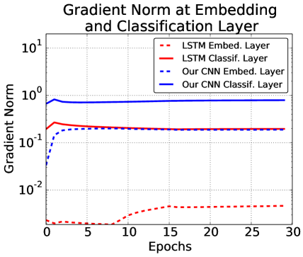
Figure 9: Here, we plot the gradient norm at the input embedding (first) and output embedding (last/classification) layer. The gradient to the first layer of LSTM decays by a factor $\sim 100$ in contrast to our CNN, where it decays by a factor of $\sim 10$. There is prior evidence in literature that unlike CNNs, RNN/LSTMs suffer from vanishing gradients [25, 33]. Here, we use solid line for input embedding layer and dotted line for the classification layer.

7 Related Work

Describing the content of an observed image is related to a large variety of tasks. Object detection [26, 27] and semantic segmentation [22, 29] can be used to obtain a list of objects. Detection of co-occurrence patterns and relationships between objects can help to form sentences. Generating sentences by taking advantage of surrogate tasks is then a multi-step approach which is beneficial for interpretability but lacks a joint objective that can be trained end-to-end.

Early techniques formulate image captioning as a retrieval problem and find the best fitting description from a pool of possible captions [12, 15, 23, 32]. Those techniques are built upon the idea that the fitness between available textual descriptions and images can be learned. While this permits end-to-end training, matching image descriptors to a sufficiently large pool of captions is computationally expensive. In addition, constructing a database of captions that is sufficient for describing a reasonably large fraction of images seems prohibitive.

To address this issue, recurrent neural nets (RNNs) or probabilistic models like Markov chains, which decompose the space of a caption into a product space of individual words are compelling. The success of RNNs for image captioning is based on a key component, i.e., the Long-Short-Term-Memory (LSTM) [11] or recent alternatives like the gated recurrent unit (GRU) [6]. These components capture long-term dependencies by adding a memory cell, and they address the vanishing or exploding gradient issue of classical RNNs to some degree.

Based on this success, [20] train a vision (or image) CNN and a language RNN that shares a joint embedding layer. [38] jointly train a vision (or image) CNN with a language RNN to generate sentences, [39] extends [38] with additional attention parameters and learns to identify salient objects for caption generation. [16] use a bi-directional RNN along with a structured loss function in a shared vision-language space. These recurrent neural nets have found widespread use for captioning because they have been shown to produce remarkably fitting descriptions.

Despite the fact that the above RNNs based on LSTM or GRU units deliver remarkable results, e.g., for image captioning, their training procedure is all but trivial. For instance, while the forward pass during training can be parallelized across samples, it is inherently sequential in time, limiting the parallelization abilities. To address this issue, [34] proposed a PixelCNN architecture for conditional image generation that approximates an RNN for the same task. [9] and [35] demonstrate that convolutional architectures with attention achieve state-of-the-art performance on machine translation tasks. In spirit similar is our approach for image captioning, which is convolutional but addresses a different task.

8 Conclusion

We discussed a convolutional approach for image captioning and showed that it performs on par with existing LSTM techniques. We also analyzed the differences between RNN based learning and our method, and found gradients of lower magnitude as well as overly confident predictions to be existing LSTM network concerns.

9 Acknowledgments

We thank Arun Mallya for providing us with an efficient PyTorch implementation of [16], we thank Tanmay Gangwani for the beam search code used for Figure 8 and we thank David Forsyth for insightful discussions and his comments. This material is based upon work supported in part by the National Science Foundation under Grant No. 1718221.

References

- [1] P. Anderson, B. Fernando, M. Johnson, and S. Gould. Spice: Semantic propositional image caption evaluation. In ECCV, 2016.
- [2] S. Antol, A. Agrawal, J. Lu, M. Mitchell, D. Batra, C. L. Zitnick, and D. Parikh. VQA: Visual Question Answering. In International Conference on Computer Vision (ICCV), 2015.
- [3] D. Bahdanau, K. Cho, and Y. Bengio. Neural machine translation by jointly learning to align and translate. CoRR, abs/1409.0473, 2014.
- [4] S. Bengio, O. Vinyals, N. Jaitly, and N. Shazeer. Scheduled sampling for sequence prediction with recurrent neural networks. In Proceedings of the 28th International Conference on Neural Information Processing Systems - Volume 1, NIPS’15, pages 1171–1179, Cambridge, MA, USA, 2015. MIT Press.
- [5] X. Chen and C. L. Zitnick. Mind’s eye: A recurrent visual representation for image caption generation. In 2015 IEEE Conference on Computer Vision and Pattern Recognition (CVPR), pages 2422–2431, June 2015.
- [6] K. Cho, B. van Merriënboer, Ç. Gülçehre, D. Bahdanau, F. Bougares, H. Schwenk, and Y. Bengio. Learning phrase representations using rnn encoder–decoder for statistical machine translation. In Proceedings of the 2014 Conference on Empirical Methods in Natural Language Processing (EMNLP), pages 1724–1734, Doha, Qatar, Oct. 2014. Association for Computational Linguistics.
- [7] A. Das, S. Kottur, K. Gupta, A. Singh, D. Yadav, J. M. F. Moura, D. Parikh, and D. Batra. Visual dialog. 2017.
- [8] M. Denkowski and A. Lavie. Meteor universal: Language specific translation evaluation for any target language. In Proceedings of the EACL 2014 Workshop on Statistical Machine Translation, 2014.
- [9] J. Gehring, M. Auli, D. Grangier, D. Yarats, and Y. N. Dauphin. Convolutional sequence to sequence learning. CoRR, abs/1705.03122, 2017.
- [10] A. Goyal, A. Lamb, Y. Zhang, S. Zhang, A. Courville, and Y. Bengio. Professor forcing: A new algorithm for training recurrent networks. pages 4601–4609. 2016.
- [11] S. Hochreiter and J. Schmidhuber. Long short-term memory. Neural Comput., 9(8):1735–1780, Nov. 1997.
- [12] M. Hodosh, P. Young, and J. Hockenmaier. Framing image description as a ranking task: Data, models and evaluation metrics. J. Artif. Int. Res., 47(1), May 2013.
- [13] T. K. Huang, F. Ferraro, N. Mostafazadeh, I. Misra, A. Agrawal, J. Devlin, R. B. Girshick, X. He, P. Kohli, D. Batra, C. L. Zitnick, D. Parikh, L. Vanderwende, M. Galley, and M. Mitchell. Visual storytelling. CoRR, abs/1604.03968, 2016.
- [14] U. Jain, Z. Zhang, and A. G. Schwing. Creativity: Generating diverse questions using variational autoencoders. In Computer Vision and Pattern Recognition, 2017.
- [15] Y. Jia, M. Salzmann, and T. Darrell. Learning cross-modality similarity for multinomial data. In Proceedings of the 2011 International Conference on Computer Vision, ICCV ’11, pages 2407–2414, Washington, DC, USA, 2011. IEEE Computer Society.
- [16] A. Karpathy and L. Fei-Fei. Deep visual-semantic alignments for generating image descriptions. In 2015 IEEE Conference on Computer Vision and Pattern Recognition (CVPR), pages 3128–3137, June 2015.
- [17] C.-Y. Lin. Rouge: a package for automatic evaluation of summaries. July 2004.
- [18] T.-Y. Lin, M. Maire, S. Belongie, J. Hays, P. Perona, D. Ramanan, P. Dollár, and C. L. Zitnick. Microsoft COCO: Common Objects in Context, pages 740–755. Springer International Publishing, Cham, 2014.
- [19] A. Mallya and S. Lazebnik. Recurrent models for situation recognition. In ICCV, 2017.
- [20] J. Mao, W. Xu, Y. Yang, J. Wang, and A. L. Yuille. Deep captioning with multimodal recurrent neural networks (m-rnn). CoRR, abs/1412.6632, 2014.
- [21] N. Mostafazadeh, I. Misra, J. Devlin, M. Mitchell, X. He, and L. Vanderwende. Generating natural questions about an image. In ACL (1). The Association for Computer Linguistics, 2016.
- [22] M. Mostajabi, P. Yadollahpour, and G. Shakhnarovich. Feedforward semantic segmentation with zoom-out features. In 2015 IEEE Conference on Computer Vision and Pattern Recognition (CVPR), pages 3376–3385, June 2015.
- [23] V. Ordonez, G. Kulkarni, and T. L. Berg. Im2text: Describing images using 1 million captioned photographs. In Proceedings of the 24th International Conference on Neural Information Processing Systems, NIPS’11, pages 1143–1151, USA, 2011. Curran Associates Inc.
- [24] K. Papineni, S. Roukos, T. Ward, and W.-J. Zhu. Bleu: A method for automatic evaluation of machine translation. In Proceedings of the 40th Annual Meeting on Association for Computational Linguistics, ACL ’02, pages 311–318, Stroudsburg, PA, USA, 2002. Association for Computational Linguistics.
- [25] R. Pascanu, T. Mikolov, and Y. Bengio. On the difficulty of training recurrent neural networks. In Proceedings of the 30th International Conference on International Conference on Machine Learning - Volume 28, ICML’13, pages III–1310–III–1318. JMLR.org, 2013.
- [26] J. Redmon, S. K. Divvala, R. B. Girshick, and A. Farhadi. You only look once: Unified, real-time object detection. CoRR, abs/1506.02640, 2015.
- [27] S. Ren, K. He, R. Girshick, and J. Sun. Faster r-cnn: Towards real-time object detection with region proposal networks. In Proceedings of the 28th International Conference on Neural Information Processing Systems - Volume 1, NIPS’15, pages 91–99, Cambridge, MA, USA, 2015. MIT Press.
- [28] O. Russakovsky, J. Deng, H. Su, J. Krause, S. Satheesh, S. Ma, Z. Huang, A. Karpathy, A. Khosla, M. Bernstein, A. C. Berg, and L. Fei-Fei. Imagenet large scale visual recognition challenge. International Journal of Computer Vision, 115(3):211–252, Dec 2015.
- [29] E. Shelhamer, J. Long, and T. Darrell. Fully convolutional networks for semantic segmentation. IEEE Trans. Pattern Anal. Mach. Intell., 39(4):640–651, Apr. 2017.
- [30] K. J. Shih, S. Singh, and D. Hoiem. Where to look: Focus regions for visual question answering. In Computer Vision and Pattern Recognition, 2016.
- [31] K. Simonyan and A. Zisserman. Very deep convolutional networks for large-scale image recognition. CoRR, abs/1409.1556, 2014.
- [32] R. Socher, A. Karpathy, Q. Le, C. Manning, and A. Ng. Grounded compositional semantics for finding and describing images with sentences. Transactions of the Association for Computational Linguistics, 2:207–218, 2014.
- [33] I. Sutskever, J. Martens, and G. Hinton. Generating text with recurrent neural networks. In L. Getoor and T. Scheffer, editors, Proceedings of the 28th International Conference on Machine Learning (ICML-11), ICML ’11, pages 1017–1024, New York, NY, USA, June 2011. ACM.
- [34] A. van den Oord, N. Kalchbrenner, O. Vinyals, L. Espeholt, A. Graves, and K. Kavukcuoglu. Conditional image generation with pixelcnn decoders. In NIPS, 2016.
- [35] A. Vaswani, N. Shazeer, N. Parmar, J. Uszkoreit, L. Jones, A. N. Gomez, L. Kaiser, and I. Polosukhin. Attention is all you need. CoRR, abs/1706.03762, 2017.
- [36] R. Vedantam, C. L. Zitnick, and D. Parikh. Cider: Consensus-based image description evaluation. In CVPR, pages 4566–4575. IEEE Computer Society, 2015.
- [37] S. Venugopalan, H. Xu, J. Donahue, M. Rohrbach, R. Mooney, and K. Saenko. Translating videos to natural language using deep recurrent neural networks. In NAACL HLT, 2015.
- [38] K. Xu, J. Ba, R. Kiros, K. Cho, A. Courville, R. Salakhudinov, R. Zemel, and Y. Bengio. Show, attend and tell: Neural image caption generation with visual attention. In F. Bach and D. Blei, editors, Proceedings of the 32nd International Conference on Machine Learning, volume 37 of Proceedings of Machine Learning Research, pages 2048–2057, Lille, France, 07–09 Jul 2015. PMLR.
- [39] K. Xu, J. L. Ba, R. Kiros, K. Cho, A. Courville, R. Salakhutdinov, R. S. Zemel, and Y. Bengio. Show, attend and tell: Neural image caption generation with visual attention. In Proceedings of the 32Nd International Conference on International Conference on Machine Learning - Volume 37, ICML’15, pages 2048–2057. JMLR.org, 2015.
- [40] Y. Yang, C. L. Teo, H. Daumé, III, and Y. Aloimonos. Corpus-guided sentence generation of natural images. In Proceedings of the Conference on Empirical Methods in Natural Language Processing, EMNLP ’11, pages 444–454, Stroudsburg, PA, USA, 2011. Association for Computational Linguistics.