Asymptotic Analysis via Stochastic Differential Equations of Gradient Descent Algorithms in Statistical and Computational Paradigms

Yazhen Wang
Department of Statistics, University of Wisconsin-Madison
Madison, WI 53706, USA. Email: yzwang@stat.wisc.edu
Abstract

This paper investigates asymptotic behaviors of gradient descent algorithms (particularly accelerated gradient descent and stochastic gradient descent) in the context of stochastic optimization arising in statistics and machine learning where objective functions are estimated from available data. We show that these algorithms can be computationally modeled by continuous-time ordinary or stochastic differential equations. We establish gradient flow central limit theorems to describe the limiting dynamic behaviors of these computational algorithms and the large-sample performances of the related statistical procedures, as the number of algorithm iterations and data size both go to infinity, where the gradient flow central limit theorems are governed by some linear ordinary or stochastic differential equations like time-dependent Ornstein-Uhlenbeck processes. We illustrate that our study can provide a novel unified framework for a joint computational and statistical asymptotic analysis, where the computational asymptotic analysis studies dynamic behaviors of these algorithms with the time (or the number of iterations in the algorithms), the statistical asymptotic analysis investigates large sample behaviors of the statistical procedures (like estimators and classifiers) that the algorithms are applied to compute, and in fact the statistical procedures are equal to the limits of the random sequences generated from these iterative algorithms as the number of iterations goes to infinity. The joint analysis results based on the obtained gradient flow central limit theorems can identify four factors – learning rate, batch size, gradient covariance, and Hessian – to derive new theory regarding the local minima found by stochastic gradient descent for solving non-convex optimization problems.

Key words: Gradient flow central limit theorem; joint computational and statistical asymptotic analysis, weak convergence limit, mini-batch, optimization, ordinary or stochastic differential equation,

Running title: Computational & Statistical Analysis of Gradient Descent

1 Introduction

1.1 Background and Motivation

Optimization plays an important role in scientific fields ranging from machine learning to physical sciences and statistics to engineering. It lies at the core of data science by providing a mathematical language for handling both computational algorithms and statistical inferences in data analysis. Numerous algorithms and methods have been proposed to solve optimization problems. Examples include Newton’s method, gradient and subgradient descent, conjugate gradient methods, trust region methods, and interior point methods (see Polyak, 1987; Boyd and Vandenberghe, 2004; Nocedal and Wright, 2006; Ruszczynski, 2006; Boyd et al., 2011; Shor, 2012; Goodfellow et al. (2016) for expositions). Practical problems arising in fields like statistics and machine learning usually involve optimization settings where the objective functions are empirically estimated from available data with the form of a sum of differentiable functions. We refer to such optimization problems with random objective functions as stochastic optimization. As data sets in practical problems grow rapidly in scale and complexity, methods such as stochastic gradient descent can scale to the enormous size of big data and have been very popular. There has been recent surging interest in and great research work on the theory and practice of gradient descent and its extensions and variants. For example, a number of recent papers were devoted to investigate stochastic gradient descent and its variants for solving complex optimization problems (Ali et al. (2019), Chen et al. (2016), Ge et al. (2015), Jin et al. (2017), Kawaguchi (2016), Keskar et al. (2017), Lee et al. (2016), Li et al. (2017b), Mandt et al. (2016), and Shallue et al. (2019)). In particular Su et al. (2016) derived the continuous-time limit of Nesterov’s accelerated gradient descent as a second-order ordinary differential equation for studying the acceleration phenomenon and generalizing Nesterov’s scheme. Wibisono et al. (2016) further developed a systematic approach based on continuous-time variations to understand the acceleration phenomenon and produce acceleration algorithms from continuous-time differential equations. In spite of compelling theoretical and numerical evidence on the value of the stochastic approximation idea and acceleration phenomenon, yet there remains some conceptual and theoretical mystery in the acceleration and stochastic approximation schemes.

1.2 Contributions

This paper establishes asymptotic theory for gradient descent, stochastic gradient descent, and accelerated gradient descent in the stochastic optimization setup. We derive continuous-time ordinary or stochastic differential equations to model the dynamic behaviors of these gradient descent algorithms and investigate their limiting algorithmic dynamics and large sample performances as the number of algorithm iterations and data size both go to infinity. Specifically for an optimization problem whose objective function is convex and deterministic, we consider a matched stochastic optimization problem whose random objective function is an empirical estimator of the deterministic objective function based on available data. The solution of the stochastic optimization specifies a decision rule like an estimator or a classifier based on the sampled data in statistics and machine learning, while its corresponding deterministic optimization problem characterizes through its solution the true value of the parameter in the population model. In other words, the two connected optimization problems associate with the data sample and its corresponding population model where the data are sampled from, and the stochastic optimization is considered to be a sample version of the deterministic optimization corresponding to the population. These two types of optimization problems refer to the deterministic population and stochastic sample optimization problems. Consider random sequences that are generated from the gradient descent algorithms and their corresponding continuous-time ordinary or stochastic differential equations for the stochastic sample optimization setting. We show that the random sequences converge to the ordinary differential equations for the corresponding deterministic population optimization setup, and we derive their asymptotic distributions by some linear ordinary or stochastic differential equations such as time-dependent Ornstein-Uhlenbeck processes. The asymptotic distributions are used to understand and quantify the limiting discrepancy between the random sequences generated from each algorithm for solving the corresponding sample and population optimization problems. In particular since the obtained asymptotic distributions characterize the limiting behavior of the normalized difference between the sample and population gradient (or Lagrangian) flows, the limiting distributions may be viewed as central limit theorems (CLT) for gradient (or Lagrangian) flows, and are then called the gradient (or Lagrangian) flow central limit theorems (GF-CLT or LF-CLT). Moreover, our analysis may offer a novel unified framework to carry out a joint asymptotic analysis for computational algorithms and statistical decision rules that the algorithms are applied to compute. As iterated computational methods, these gradient descent algorithms generate sequences that converge to the exact decision rule or the true parameter value for the corresponding optimization problems, when the number of the iterations goes to infinity. Thus, as time (corresponding to the number of iterations) goes to infinity, the continuous-time differential equations may have distributional limits corresponding to the large-sample distributions of statistical decision rules as the sample size goes to infinity. In other words, the asymptotic analysis can be done with both time and data size, where the time direction corresponds to the computational asymptotics on dynamic behaviors of the algorithms, and the data size direction associates with the statistical large-sample asymptotics on the statistical behaviors of decision rules such as estimators and classifiers. The continuous-time modeling and the GF-CLT based joint asymptotic analysis may reveal new facts and shed some light on the phenomenon that stochastic gradient descent algorithms can escape from saddle points and converge to good local minimizers for solving non-convex optimization problems in deep learning. To the best of our knowledge, this is the first paper to establish the GF-CLT and LF-CLT, offer the unified framework for the joint computational and statistical asymptotic analysis, and establish a novel theory to identify four factors for influencing the local minima found by stochastic gradient descent in non-convex optimization.

There is a large literature on stochastic approximation and recursive algorithms in particular stochastic gradient descent in deep learning (see Chen et al. (2016), Dalalyan (2017), Fan et al. (2018), Ge et al. (2015), Jastrzȩbski et al. (2018), Jin et al. (2017), Kawaguchi (2016), Keskar et al. (2017), Kushner and Yin (2003), Lee et al. (2016), Li et al. (2016), Li et al. (2017a), Li et al. (2017b), Ma et al. (2019), Mandt et al. (2016), Shallue et al. (2019), Sirignano and Spiliopoulos (2017), Su et al. (2016), Wibisono et al. (2016)). Both continuous-time and discrete-time means are adopted by computational and statistical (as well as machine learning) communities. The work on the computational side focuses more on the dynamics and convergence of learning algorithms, while the statistics research emphasizes more on statistical inferences of learning rules. Our study combines both computational and statistical approaches to carry out a joint analysis on the learning algorithms and the learning rules, where the algorithms are used to compute the rules. In a nutshell, we analyze the learning algorithms in terms of both computational dynamic convergence behavior and statistical large sample performance. The developed GF-CLT based theory and the created joint analysis provide a description of dynamic convergence behaviors of the computational algorithms as well as the statistical large sample performances of the learning rules computed by the algorithms. The statistical behaviors of the associated learning rules can be derived from the GF-CLT at an infinite time horizon. On the computational side, it has implications for optimization phenomena observed in the discrete-time case as well as in practice. For example, the obtained GF-CLT uncovers that the gradient flow for the stochastic sample optimization can be decomposed into the gradient flow for the corresponding deterministic population optimization plus a random fluctuation term, where the random fluctuation depends on the learning rate and batch size only through their ratio and is governed by a time-dependent Ornstein-Uhlenbeck process. Using the joint analysis along with the algebraic Ricatti equation for characterizing the stationary covariance of the Ornstein-Uhlenbeck process, we discover a novel theory about how the minima found by stochastic gradient descent are influenced by four factors: learning rate, batch size, gradient covariance, and Hessian. As a case in point, our general results cover the study under a special circumstance in Jastrzȩbski et al. (2018) that can identify only three of the four factors to influence the local minima found by stochastic gradient descent. Foster et al. (2019) showed that the complexity of a stochastic optimization can be decomposed into the complexity of its corresponding deterministic population optimization and the sample complexity, where the optimization complexity represents the minimal amount of effort required to find near-stationary points, and the sample complexity of an algorithm refers to the number of training-samples needed to learn a target function sufficient well. Our results indicate that finding near-stationary points for a stochastic sample optimization can be converted into finding near-stationary points for the corresponding deterministic population optimization plus some control on the random fluctuation term. As the random fluctuation has zero mean, the control can be achieved through bounding the variance of the time-dependent Ornstein-Uhlenbeck process along with selecting a sufficiently small ratio of learning rate to batch size, which is often used to describe the sample complexity of the associated statistical learning problem for the time-dependent Ornstein-Uhlenbeck process. This shows that our results are in agreement with Foster et al. (2019), and may point to some potential intrinsic connection between our approach and that in Foster et al. (2019). Furthermore, the continuous-time approach serves as a handy means as well as a beautiful framework to formulate stochastic dynamics and statistical procedures and derive their limiting behaviors and large sample performances. These are eventually used to establish limiting behaviors of their discrete counterparts.

In summary, we highlight our main contributions as follows:

  • We establish a new asymptotic theory for the discrepancy between the sample and population gradient (or Lagrangian) flows. In particular the new limiting distributions for the normalized discrepancy are called the gradient (or Lagrangian) flow central limit theorems (GF-CLT or LF-CLT). See Sections 3.3 and 4.1-4.2.

  • The obtained asymptotic theory provides a novel unified framework for a joint computational and statistical asymptotic analysis. Statistically the joint analysis can facilitate inferential analysis of a learning rule computed by gradient descent algorithms. Computationally the joint analysis enables us to understand and quantify a random fluctuation in and the related impact on the dynamic and convergence behavior of a gradient descent algorithm when being applied to solve a stochastic optimization problem. See Sections 3.4 and 4.3.

  • Computationally we discover a novel theory that four factors – learning rate, batch size, gradient covariance, and Hessian – along with the associated identities are shown to influence the local minima found by stochastic gradient descent for solving a non-convex optimization problem. It may also shed light on some intrinsic relationship among stochastic optimization, deterministic optimization, and statistical learning. See Section 4.4.

  • Statistically we illustrate implications of our results for statistical analysis of stochastic gradient descent and inference of outputs from stochastic gradient descent. See Section 4.5.

  • The continuous-time approach is employed to demonstrate that it can provide a handy means for deriving beautiful and deep results for stochastic dynamics of learning algorithms and statistical inference of learning rules.

1.3 Organization

The rest of the paper proceeds as follows. Section 2 introduces gradient descent, accelerated gradient descent, and their corresponding ordinary differential equations. Section 3 presents stochastic optimization and investigates asymptotic behaviors of the plain and accelerated gradient descent algorithms and their associated ordinary differential equations (with random coefficients) when the sample size goes to infinity. We illustrate the unified framework to carry out a joint analysis on computational and statistical asymptotics, where computational asymptotics deals with dynamic behaviors of the gradient descent algorithms with time (or iteration), and statistical asymptotics studies large sample behaviors of statistical decision rules that the algorithms are applied to compute. Section 4 considers stochastic gradient descent algorithms for large scale data and derives stochastic differential equations to model these algorithms. We establish asymptotic theory for these algorithms and their associated stochastic differential equations, and describe a joint analysis on computational and statistical asymptotics. Section 5 features an example. All technical proofs are relegated in the appendix section.

We adopt the following notations and conventions. For the stochastic sample optimization problem considered in Sections 3 and 4, we add a superscript n𝑛n to notations for the associated processes and sequences in Section 3 and indices m𝑚m and/or * to notations for the corresponding processes and sequences affiliated with mini-batches in Section 4, while notations without such subscripts or superscripts are for sequences and functions corresponding to the deterministic population optimization problem given in Section 2. Our basic proof ideas are as follows. Each algorithm generates a sequence for computing a learning rule, a step-wise empirical process is formed by the generated sequence, and a continuous process is obtained from the corresponding continuous-time differential equation. We derive asymptotic distributions by analyzing the differential equations, and we bound the differences between the empirical processes and their corresponding continuous processes by studying the optimization problems and utilizing the empirical process theory along with the related differential equations.

2 Ordinary differential equations for gradient descent algorithms

Consider the following minimization problem

minθΘg(θ),subscript𝜃Θ𝑔𝜃\min_{\theta\in\Theta}g(\theta), (2.1)

where the objective function g(θ)𝑔𝜃g(\theta) is defined on a parameter space ΘIRpΘ𝐼superscript𝑅𝑝\Theta\subset I\!\!R^{p} and assumed to have L-Lipshitz continuous gradients. Iterative algorithms such as gradient descent methods are often employed to numerically compute the solution of the minimization problem. Starting with some initial values x0subscript𝑥0x_{0}, the plain gradient descent algorithm is iteratively defined by

xk=xk1δg(xk1),subscript𝑥𝑘subscript𝑥𝑘1𝛿𝑔subscript𝑥𝑘1\displaystyle x_{k}=x_{k-1}-\delta\nabla\!g(x_{k-1}), (2.2)

where \nabla denotes gradient operator, and δ𝛿\delta is a positive constant which is often called a step size or learning rate.

It is easy to model {xk\{x_{k}, k=0,1,}k=0,1,\cdots\} by a smooth curve X(t)𝑋𝑡X(t) with the Ansatz xkX(kδ)subscript𝑥𝑘𝑋𝑘𝛿x_{k}\approx X(k\delta) as follows. Define a step function xδ(t)=xksubscript𝑥𝛿𝑡subscript𝑥𝑘x_{\delta}(t)=x_{k} for kδt<(k+1)δ𝑘𝛿𝑡𝑘1𝛿k\delta\leq t<(k+1)\delta, and as δ0𝛿0\delta\rightarrow 0, xδ(t)subscript𝑥𝛿𝑡x_{\delta}(t) approaches X(t)𝑋𝑡X(t) satisfying

X˙(t)+g(X(t))=0,˙𝑋𝑡𝑔𝑋𝑡0\dot{X}(t)+\nabla g(X(t))=0, (2.3)

where X˙(t)˙𝑋𝑡\dot{X}(t) denotes the derivative of X(t)𝑋𝑡X(t), and initial value X(0)=x0𝑋0subscript𝑥0X(0)=x_{0}. In fact, X(t)𝑋𝑡X(t) is a gradient flow associated with the objective function g()𝑔g(\cdot) in the optimization problem (2.1).

Nesterov’s accelerated gradient descent scheme is a well-known algorithm that is much faster than the plain gradient descent algorithm. Starting with initial values x0subscript𝑥0x_{0} and y0=x0subscript𝑦0subscript𝑥0y_{0}=x_{0}, Nesterov’s accelerated gradient descent algorithm is iteratively defined by

xk=yk1δg(yk1),yk=xk+k1k+2(xkxk1),formulae-sequencesubscript𝑥𝑘subscript𝑦𝑘1𝛿𝑔subscript𝑦𝑘1subscript𝑦𝑘subscript𝑥𝑘𝑘1𝑘2subscript𝑥𝑘subscript𝑥𝑘1\displaystyle x_{k}=y_{k-1}-\delta\nabla\!g(y_{k-1}),\qquad y_{k}=x_{k}+\frac{k-1}{k+2}(x_{k}-x_{k-1}), (2.4)

where δ𝛿\delta is a positive constant. Using (2.4) we derive a recursive relationship between consecutive increments

xk+1xkδ=k1k+2xkxk1δδg(yk).subscript𝑥𝑘1subscript𝑥𝑘𝛿𝑘1𝑘2subscript𝑥𝑘subscript𝑥𝑘1𝛿𝛿𝑔subscript𝑦𝑘\frac{x_{k+1}-x_{k}}{\sqrt{\delta}}=\frac{k-1}{k+2}\frac{x_{k}-x_{k-1}}{\sqrt{\delta}}-\sqrt{\delta}\nabla\!g(y_{k}). (2.5)

We model {xk\{x_{k}, k=0,1,}k=0,1,\cdots\} by a smooth curve in a sense that xksubscript𝑥𝑘x_{k} are its samples at discrete points, that is, we define a step function xδ(t)=xksubscript𝑥𝛿𝑡subscript𝑥𝑘x_{\delta}(t)=x_{k} for kδt<(k+1)δ𝑘𝛿𝑡𝑘1𝛿k\sqrt{\delta}\leq t<(k+1)\sqrt{\delta}, and introduce the Ansatz xδ(kδ)=xkX(kδ)subscript𝑥𝛿𝑘𝛿subscript𝑥𝑘𝑋𝑘𝛿x_{\delta}(k\sqrt{\delta})=x_{k}\approx X(k\sqrt{\delta}) for some smooth function X(t)𝑋𝑡X(t) defined for t0𝑡0t\geqslant 0. Let δ𝛿\sqrt{\delta} be the step size. For t=kδ𝑡𝑘𝛿t=k\sqrt{\delta}, as δ0𝛿0\delta\rightarrow 0, we have xk=xt/δ=X(t)subscript𝑥𝑘subscript𝑥𝑡𝛿𝑋𝑡x_{k}=x_{t/\sqrt{\delta}}=X(t), xk+1=x(t+δ)/δ=X(t+δ)subscript𝑥𝑘1subscript𝑥𝑡𝛿𝛿𝑋𝑡𝛿x_{k+1}=x_{(t+\sqrt{\delta})/\sqrt{\delta}}=X(t+\sqrt{\delta}), and

yk=X(t)+t/δ1t/δ+2[X(t)X(tδ)]=X(t)+O(δ).subscript𝑦𝑘𝑋𝑡𝑡𝛿1𝑡𝛿2delimited-[]𝑋𝑡𝑋𝑡𝛿𝑋𝑡𝑂𝛿\displaystyle y_{k}=X(t)+\frac{t/\sqrt{\delta}-1}{t/\sqrt{\delta}+2}[X(t)-X(t-\sqrt{\delta})]=X(t)+O(\sqrt{\delta}).

Applying the Taylor expansion and using L-Lipshitz continuous gradients we obtain

xk+1xkδ=X(t+δ)X(t)δ=X˙(t)+12X¨(t)δ+o(δ),subscript𝑥𝑘1subscript𝑥𝑘𝛿𝑋𝑡𝛿𝑋𝑡𝛿˙𝑋𝑡12¨𝑋𝑡𝛿𝑜𝛿\frac{x_{k+1}-x_{k}}{\sqrt{\delta}}=\frac{X(t+\sqrt{\delta})-X(t)}{\sqrt{\delta}}=\dot{X}(t)+\frac{1}{2}\ddot{X}(t)\sqrt{\delta}+o(\sqrt{\delta}),
xkxk1δ=X(t)X(tδ)δ=X˙(t)12X¨(t)δ+o(δ),subscript𝑥𝑘subscript𝑥𝑘1𝛿𝑋𝑡𝑋𝑡𝛿𝛿˙𝑋𝑡12¨𝑋𝑡𝛿𝑜𝛿\frac{x_{k}-x_{k-1}}{\sqrt{\delta}}=\frac{X(t)-X(t-\sqrt{\delta})}{\sqrt{\delta}}=\dot{X}(t)-\frac{1}{2}\ddot{X}(t)\sqrt{\delta}+o(\sqrt{\delta}),
δg(yk)=δg(X(t))+o(δ),𝛿𝑔subscript𝑦𝑘𝛿𝑔𝑋𝑡𝑜𝛿\sqrt{\delta}\nabla\!g(y_{k})=\sqrt{\delta}\nabla\!g(X(t))+o(\sqrt{\delta}),

where X¨(t)¨𝑋𝑡\ddot{X}(t) denotes the second derivative of X(t)𝑋𝑡X(t). Substituting above results into the equation (2.5) and letting δ0𝛿0\delta\rightarrow 0 we obtain

X¨(t)+3tX˙(t)+g(X(t))=0,¨𝑋𝑡3𝑡˙𝑋𝑡𝑔𝑋𝑡0\ddot{X}(t)+\frac{3}{t}\dot{X}(t)+\nabla\!g(X(t))=0, (2.6)

with the initial conditions X(0)=x0𝑋0subscript𝑥0X(0)=x_{0} and X˙(0)=0˙𝑋00\dot{X}(0)=0. As the coefficient 3/t3𝑡3/t in the ordinary differential equation (2.6) is singular at t=0𝑡0t=0, classical ordinary differential equation theory is not applicable to establish the existence or uniqueness of the solution to the equation (2.6). The heuristic derivation of (2.6) is from Su et al. (2016) who has established that the equation (2.6) has a unique solution satisfying the initial conditions, and xδ(t)subscript𝑥𝛿𝑡x_{\delta}(t) converges to X(t)𝑋𝑡X(t) uniformly on [0,T]0𝑇[0,T] for any fixed T>0𝑇0T>0. Note the step size difference between the plain and accelerated cases, where the step size is δ1/2superscript𝛿12\delta^{1/2} for Nesterov’s accelerated gradient descent algorithm and δ𝛿\delta for the plain gradient descent algorithm. Su et al. (2016) has shown that, because of the difference, the accelerated gradient descent algorithm moves much faster than the plain gradient descent algorithm along the curve X(t)𝑋𝑡X(t). Wibisono et al. (2016) provided more elaborate explanation on the acceleration phenomenon and developed a systematic continuous-time variational scheme to generate a large class of continuous-time differential equations and produce a family of accelerated gradient algorithms. The variational scheme utilizes a first-order rescaled gradient flow and a second-order Lagrangian flow, which are generalizations of gradient flow. As we refer the solution X(t)𝑋𝑡X(t) of the differential equation (2.3) to the gradient flow for the gradient descent algorithm (2.2), the solution X(t)𝑋𝑡X(t) to the differential equation (2.6) is called the Lagrangian flow for the accelerated gradient descent algorithm (2.4).

3 Gradient descent for stochastic optimization

Let θ=(θ1,,θp)𝜃superscriptsubscript𝜃1subscript𝜃𝑝\theta=(\theta_{1},...,\theta_{p})^{{}^{\prime}} be the parameter that we are interested in, and U𝑈U be a relevant random element on a probability space with a given distribution Q𝑄Q. Consider an objective function (θ;u)𝜃𝑢\ell(\theta;u) and its corresponding expectation E[(θ;U)]=g(θ)𝐸delimited-[]𝜃𝑈𝑔𝜃E[\ell(\theta;U)]=g(\theta). For example, in a statistical decision problem, we may take U𝑈U to be a decision rule, (θ;u)𝜃𝑢\ell(\theta;u) a loss function, and g(θ)=E[(θ;U)]𝑔𝜃𝐸delimited-[]𝜃𝑈g(\theta)=E[\ell(\theta;U)] its corresponding risk; in M-estimation, we may treat U𝑈U as a sample observation and (θ,u)𝜃𝑢\ell(\theta,u) a ρ𝜌\rho-function; in nonparametric function estimation and machine learning, we may choose U𝑈U an observation and (θ;u)𝜃𝑢\ell(\theta;u) equal to a loss function plus some penalty. For these problems we need to consider the corresponding population minimization problem (2.1) for characterizing the true parameter value or its function as an estimand, but practically, because g(θ)𝑔𝜃g(\theta) is usually unavailable, we have to employ its empirical version and consider a stochastic optimization problem, described as follows:

minθΘn(θ;𝐔n),subscript𝜃Θsuperscript𝑛𝜃subscript𝐔𝑛\min_{\theta\in\Theta}{\cal L}^{n}(\theta;{\bf U}_{n}), (3.7)

where n(θ;𝐔n)=1ni=1n(θ;Ui)superscript𝑛𝜃subscript𝐔𝑛1𝑛superscriptsubscript𝑖1𝑛𝜃subscript𝑈𝑖{\cal L}^{n}(\theta;{\bf U}_{n})=\frac{1}{n}\sum_{i=1}^{n}\ell(\theta;U_{i}), 𝐔n=(U1,,Un)subscript𝐔𝑛superscriptsubscript𝑈1subscript𝑈𝑛{\bf U}_{n}=(U_{1},\cdots,U_{n})^{\prime} is a sample, and we assume that U1,,Unsubscript𝑈1subscript𝑈𝑛U_{1},\cdots,U_{n} are i.i.d. and follow the distribution Q𝑄Q.

The minimization problem (2.1) characterizes the true value of the target estimand such as an estimation parameter in a statistical model and a classification parameter in a machine learning task. As the true objective function g(θ)𝑔𝜃g(\theta) is usually unknown in practice, we often solve the stochastic minimization problem (3.7) with observed data to obtain practically useful decision rules such as an M-estimator, a smoothing function estimator, and a machine learning classifier. The approach to obtaining practical procedures is based on the heuristic reasoning that as n𝑛n\rightarrow\infty, the law of large number implies that n(θ;𝐔n)superscript𝑛𝜃subscript𝐔𝑛{\cal L}^{n}(\theta;{\bf U}_{n}) eventually converges to g(θ)𝑔𝜃g(\theta) in probability, and thus the solution of (3.7) approaches that of the minimization problem (2.1).

3.1 Plain gradient descent algorithm

Applying the plain gradient descent scheme to the minimization problem (3.7) with initial value x0nsubscriptsuperscript𝑥𝑛0x^{n}_{0}, we obtain the following iterative algorithm to compute the solution of (3.7),

xkn=xk1nδn(xk1n;𝐔n),subscriptsuperscript𝑥𝑛𝑘subscriptsuperscript𝑥𝑛𝑘1𝛿superscript𝑛subscriptsuperscript𝑥𝑛𝑘1subscript𝐔𝑛\displaystyle x^{n}_{k}=x^{n}_{k-1}-\delta\nabla\!{\cal L}^{n}(x^{n}_{k-1};{\bf U}_{n}), (3.8)

where δ>0𝛿0\delta>0 is a step size or learning rate, and nsuperscript𝑛{\cal L}^{n} is the objective function in the minimization problem (3.7).

Following the continuous curve approximation described in Section 2 we define a step function xδn(t)=xknsubscriptsuperscript𝑥𝑛𝛿𝑡subscriptsuperscript𝑥𝑛𝑘x^{n}_{\delta}(t)=x^{n}_{k} for kδt<(k+1)δ𝑘𝛿𝑡𝑘1𝛿k\delta\leq t<(k+1)\delta, and for each n𝑛n, as δ0𝛿0\delta\rightarrow 0, xδn(t)subscriptsuperscript𝑥𝑛𝛿𝑡x^{n}_{\delta}(t) approaches a smooth curve Xn(t)superscript𝑋𝑛𝑡X^{n}(t), t0𝑡0t\geq 0, given by

X˙n(t)+n(Xn(t);𝐔n)=0,superscript˙𝑋𝑛𝑡superscript𝑛superscript𝑋𝑛𝑡subscript𝐔𝑛0\dot{X}^{n}(t)+\nabla\!{\cal L}^{n}(X^{n}(t);{\bf U}_{n})=0, (3.9)

where n(Xn(t);𝐔n)=1ni=1n(Xn(t);Ui)superscript𝑛superscript𝑋𝑛𝑡subscript𝐔𝑛1𝑛superscriptsubscript𝑖1𝑛superscript𝑋𝑛𝑡subscript𝑈𝑖\nabla\!{\cal L}^{n}(X^{n}(t);{\bf U}_{n})=\frac{1}{n}\sum_{i=1}^{n}\nabla\!\ell(X^{n}(t);U_{i}), gradient operator \nabla here is applied to n(θ;𝐔n)superscript𝑛𝜃subscript𝐔𝑛{\cal L}^{n}(\theta;{\bf U}_{n}) and (θ;Ui)𝜃subscript𝑈𝑖\ell(\theta;U_{i}) with respect to θ𝜃\theta, and initial value Xn(0)=x0nsuperscript𝑋𝑛0subscriptsuperscript𝑥𝑛0X^{n}(0)=x^{n}_{0}. Xn(t)superscript𝑋𝑛𝑡X^{n}(t) is a gradient flow associated with nsuperscript𝑛{\cal L}^{n} in the optimization problem (3.7).

As 𝐔nsubscript𝐔𝑛{\bf U}_{n} and Xn(t)superscript𝑋𝑛𝑡X^{n}(t) are random, and our main interest is to study the distributional behaviors of the solution and algorithm, we may define a solution of the equation (3.9) in a weak sense that there exist a process Xn(t)subscriptsuperscript𝑋𝑛𝑡X^{n}_{\dagger}(t) and a random vector 𝐔n=(U1,,Un)superscriptsubscript𝐔𝑛superscriptsubscriptsuperscript𝑈1subscriptsuperscript𝑈𝑛{\bf U}_{n}^{\dagger}=(U^{\dagger}_{1},\cdots,U^{\dagger}_{n})^{\prime} defined on some probability space such that 𝐔nsuperscriptsubscript𝐔𝑛{\bf U}_{n}^{\dagger} is identically distributed as 𝐔nsubscript𝐔𝑛{\bf U}_{n}, (𝐔n,Xn(t))subscriptsuperscript𝐔𝑛subscriptsuperscript𝑋𝑛𝑡({\bf U}^{\dagger}_{n},X^{n}_{\dagger}(t)) satisfies the equation (3.9), and Xn(t)subscriptsuperscript𝑋𝑛𝑡X^{n}_{\dagger}(t) is called a (weak) solution of the equation (3.9). Note that Xn(t)subscriptsuperscript𝑋𝑛𝑡X^{n}_{\dagger}(t) is not required to be defined on a fixed probability space with given random variables, instead we define Xn(t)subscriptsuperscript𝑋𝑛𝑡X^{n}_{\dagger}(t) on some probability space with some associated random variables Uisuperscriptsubscript𝑈𝑖U_{i}^{\dagger} whose distributions are given by Q𝑄Q. The weak solution definition, which shares the same spirit as that for stochastic differential equations (see Ikeda and Watanabe (1981) and more in Section 4), will be very handy in facilitating our asymptotic analysis in this paper. For simplicity we drop index \dagger and ‘weak’ when there is no confusion.

3.2 Accelerated gradient descent algorithm

Nesterov’s accelerated gradient descent scheme can be used to solve the minimization problem (3.7). Starting with initial values x0nsubscriptsuperscript𝑥𝑛0x^{n}_{0} and y0n=x0nsubscriptsuperscript𝑦𝑛0subscriptsuperscript𝑥𝑛0y^{n}_{0}=x^{n}_{0}, we obtain the following iterative algorithm to compute the solution of the stochastic minimization problem (3.7),

xkn=yk1nδn(yk1n;𝐔n),ykn=xkn+k1k+2(xknxk1n).formulae-sequencesubscriptsuperscript𝑥𝑛𝑘subscriptsuperscript𝑦𝑛𝑘1𝛿superscript𝑛subscriptsuperscript𝑦𝑛𝑘1subscript𝐔𝑛subscriptsuperscript𝑦𝑛𝑘subscriptsuperscript𝑥𝑛𝑘𝑘1𝑘2subscriptsuperscript𝑥𝑛𝑘subscriptsuperscript𝑥𝑛𝑘1\displaystyle x^{n}_{k}=y^{n}_{k-1}-\delta\nabla\!{\cal L}^{n}(y^{n}_{k-1};{\bf U}_{n}),\qquad y^{n}_{k}=x^{n}_{k}+\frac{k-1}{k+2}(x^{n}_{k}-x^{n}_{k-1}). (3.10)

Using the continuous curve approach described in Section 2 we can define a step function xδn(t)=xksubscriptsuperscript𝑥𝑛𝛿𝑡subscript𝑥𝑘x^{n}_{\delta}(t)=x_{k} for kδt<(k+1)δ𝑘𝛿𝑡𝑘1𝛿k\sqrt{\delta}\leq t<(k+1)\sqrt{\delta}, and for every n𝑛n, as δ0𝛿0\delta\rightarrow 0, we approximate xδn(t)subscriptsuperscript𝑥𝑛𝛿𝑡x^{n}_{\delta}(t) by a smooth curve Xn(t)superscript𝑋𝑛𝑡X^{n}(t), t0𝑡0t\geq 0, governed by

X¨n(t)+3tX˙n(t)+n(Xn(t);𝐔n)=0,superscript¨𝑋𝑛𝑡3𝑡superscript˙𝑋𝑛𝑡superscript𝑛superscript𝑋𝑛𝑡subscript𝐔𝑛0\ddot{X}^{n}(t)+\frac{3}{t}\dot{X}^{n}(t)+\nabla\!{\cal L}^{n}(X^{n}(t);{\bf U}_{n})=0, (3.11)

where initial values Xn(0)=x0nsuperscript𝑋𝑛0subscriptsuperscript𝑥𝑛0X^{n}(0)=x^{n}_{0} and X˙n(0)=0superscript˙𝑋𝑛00\dot{X}^{n}(0)=0, n(Xn(t);𝐔n)=1ni=1n(Xn(t);Ui)superscript𝑛superscript𝑋𝑛𝑡subscript𝐔𝑛1𝑛superscriptsubscript𝑖1𝑛superscript𝑋𝑛𝑡subscript𝑈𝑖\nabla\!{\cal L}^{n}(X^{n}(t);{\bf U}_{n})=\frac{1}{n}\sum_{i=1}^{n}\nabla\!\ell(X^{n}(t);U_{i}), and gradient operator \nabla here is applied to n(θ;𝐔n)superscript𝑛𝜃subscript𝐔𝑛{\cal L}^{n}(\theta;{\bf U}_{n}) and (θ;Ui)𝜃subscript𝑈𝑖\ell(\theta;U_{i}) with respect to θ𝜃\theta. Xn(t)superscript𝑋𝑛𝑡X^{n}(t) is a Lagrangian flow associated with nsuperscript𝑛{\cal L}^{n} in the optimization problem (3.7).

Again we define a solution Xn(t)superscript𝑋𝑛𝑡X^{n}(t) of the equation (3.11) in the weak sense, i.e., that there exist a process Xn(t)superscript𝑋𝑛𝑡X^{n}(t) and a random vector 𝐔nsubscript𝐔𝑛{\bf U}_{n} on some probability space so that the distribution of 𝐔nsubscript𝐔𝑛{\bf U}_{n} is specified by Q𝑄Q, and Xn(t)superscript𝑋𝑛𝑡X^{n}(t) is a solution of the equation (3.11).

3.3 Asymptotic theory via ordinary differential equations

To make the equations (3.9) and (3.11) and their solutions to be well defined and study their asymptotics we need to impose the following conditions.

  1. A0.

    Assume initial values satisfy x0nx0=oP(n1/2)subscriptsuperscript𝑥𝑛0subscript𝑥0subscript𝑜𝑃superscript𝑛12x^{n}_{0}-x_{0}=o_{P}(n^{-1/2}).

  2. A1.

    (θ;u)𝜃𝑢\ell(\theta;u) is continuously twice differentiable in θ𝜃\theta; for-all\forall uRp𝑢superscript𝑅𝑝u\in R^{p}, \exists h1(u)subscript1𝑢h_{1}(u), such that for-all\forall θ1,θ2Θsuperscript𝜃1superscript𝜃2Θ\theta^{1},\theta^{2}\in\Theta, (θ1;u)(θ2;u)h1(u)θ1θ2delimited-∥∥superscript𝜃1𝑢superscript𝜃2𝑢subscript1𝑢delimited-∥∥superscript𝜃1superscript𝜃2\lVert\nabla\!\ell(\theta^{1};u)-\nabla\!\ell(\theta^{2};u)\rVert\leqslant h_{1}(u)\lVert\theta^{1}-\theta^{2}\rVert, where h1(U)subscript1𝑈h_{1}(U) and (θ0;U)subscript𝜃0𝑈\nabla\ell(\theta_{0};U) for some fixed θ0subscript𝜃0\theta_{0} have finite fourth moments.

  3. A2.

    E[(θ;U)]=g(θ)𝐸delimited-[]𝜃𝑈𝑔𝜃E[\ell(\theta;U)]=g(\theta), E[(θ;U)]=g(θ)𝐸delimited-[]𝜃𝑈𝑔𝜃E[\nabla\!\ell(\theta;U)]=\nabla\!g(\theta), E[𝑰𝑯(θ;U)]=𝑰𝑯g(θ)𝐸delimited-[]𝑰𝑯𝜃𝑈𝑰𝑯𝑔𝜃E[\boldsymbol{I\!\!H}\!\ell(\theta;U)]=\boldsymbol{I\!\!H}\!g(\theta), on the parameter space ΘΘ\Theta, g()𝑔g(\cdot) is continuously twice differentiable and strongly convex, and g()𝑔\nabla g(\cdot) is L𝐿L-Lipschitz for some L>0𝐿0L>0, where \nabla is the gradient operator (the first order partial derivatives), and 𝑰𝑯𝑰𝑯\boldsymbol{I\!\!H}\! is the Hessian operator (the second order partial derivatives).

  4. A3.

    Define cross auto-covariance 𝝇(θ,ϑ)=(ςij(θ,ϑ))1i,jp𝝇𝜃italic-ϑsubscriptsubscript𝜍𝑖𝑗𝜃italic-ϑformulae-sequence1𝑖𝑗𝑝\mbox{\boldmath$\varsigma$}(\theta,\vartheta)=(\varsigma_{ij}(\theta,\vartheta))_{1\leq i,j\leq p}, θ,ϑΘ𝜃italic-ϑΘ\theta,\vartheta\in\Theta, where
    Cov[θi(θ;U),ϑj(ϑ;U)]=ςij(θ,ϑ)subscript𝜃𝑖𝜃𝑈subscriptitalic-ϑ𝑗italic-ϑ𝑈subscript𝜍𝑖𝑗𝜃italic-ϑ[\frac{\partial}{\partial\theta_{i}}\ell(\theta;U),\frac{\partial}{\partial\vartheta_{j}}\ell(\vartheta;U)]=\varsigma_{ij}(\theta,\vartheta) are assumed to be continuously differentiable, and L𝐿L-Lipschitz. Let σij(θ)=subscript𝜎𝑖𝑗𝜃absent\sigma_{ij}(\theta)= Cov[θi(θ;U),θj(θ;U)]=ςij(θ,θ)subscript𝜃𝑖𝜃𝑈subscript𝜃𝑗𝜃𝑈subscript𝜍𝑖𝑗𝜃𝜃[\frac{\partial}{\partial\theta_{i}}\ell(\theta;U),\frac{\partial}{\partial\theta_{j}}\ell(\theta;U)]=\varsigma_{ij}(\theta,\theta), and 𝝈2(θ)=superscript𝝈2𝜃absent\mbox{\boldmath$\sigma$}^{2}(\theta)= Var[(θ;U)]=(σij(θ))1i,jp=𝝇(θ,θ)delimited-[]𝜃𝑈subscriptsubscript𝜎𝑖𝑗𝜃formulae-sequence1𝑖𝑗𝑝𝝇𝜃𝜃[\nabla\!\ell(\theta;U)]=(\sigma_{ij}(\theta))_{1\leq i,j\leq p}=\mbox{\boldmath$\varsigma$}(\theta,\theta) be positive definite.

  5. A4.

    n[n(θ;𝐔n)g(θ)]=1ni=1n[(θ;Ui)g(θ)]𝑛delimited-[]superscript𝑛𝜃subscript𝐔𝑛𝑔𝜃1𝑛superscriptsubscript𝑖1𝑛delimited-[]𝜃subscript𝑈𝑖𝑔𝜃\sqrt{n}[\nabla\!{\cal L}^{n}(\theta;{\bf U}_{n})-\nabla\!g(\theta)]=\frac{1}{\sqrt{n}}\sum_{i=1}^{n}[\nabla\ell(\theta;U_{i})-\nabla g(\theta)] weakly converges to 𝐙(θ)𝐙𝜃{\bf Z}(\theta) uniformly over θΘX𝜃subscriptΘ𝑋\theta\in\Theta_{X}, where 𝐙(θ)𝐙𝜃{\bf Z}(\theta) is a Gaussian process with mean zero and auto-covariance 𝝇(θ,ϑ)𝝇𝜃italic-ϑ\mbox{\boldmath$\varsigma$}(\theta,\vartheta) defined in A3, ΘXsubscriptΘ𝑋\Theta_{X} is a bounded subset of ΘΘ\Theta, and the interior of ΘXsubscriptΘ𝑋\Theta_{X} contains the solutions X(t)𝑋𝑡X(t) of the ordinary differential equations (2.3) and (2.6) connecting the initial value x0subscript𝑥0x_{0} and the minimizer of g(θ)𝑔𝜃g(\theta).

Conditions A1-A2 are often used to make optimization problems and differential equations to be well defined, and match the stochastic sample optimization problem (3.7) to the deterministic population optimization problem (2.1). Conditions A3-A4 guarantee that the solution of (3.7) and its associated differential equations provide large sample approximations of those for (2.1). Condition A4 can be easily justified by empirical processes with common assumptions such as that (θ;U)𝜃𝑈\nabla\!\ell(\theta;U), θΘX𝜃subscriptΘ𝑋\theta\in\Theta_{X}, form a Donsker class (van der Vaart and Wellner (2000)), since the solution curves X(t)𝑋𝑡X(t) of the ordinary differential equations (2.3) and (2.6) are deterministic and bounded, and it is easy to select ΘXsubscriptΘ𝑋\Theta_{X}.

For a given T>0𝑇0T>0, denote by C([0,T])𝐶0𝑇C([0,T]) the space of all continuous functions on [0,T]0𝑇[0,T] with the uniform metric max{|b1(t)b2(t)|:t[0,T]}:subscript𝑏1𝑡subscript𝑏2𝑡𝑡0𝑇\max\{|b_{1}(t)-b_{2}(t)|:t\in[0,T]\} between functions b1(t)subscript𝑏1𝑡b_{1}(t) and b2(t)subscript𝑏2𝑡b_{2}(t). For the solutions X(t)𝑋𝑡X(t) and Xn(t)superscript𝑋𝑛𝑡X^{n}(t) of the ordinary differential equations (2.3) and (3.9) [or (2.6) and (3.11)], respectively, we define Vn(t)=n[Xn(t)X(t)]superscript𝑉𝑛𝑡𝑛delimited-[]superscript𝑋𝑛𝑡𝑋𝑡V^{n}(t)=\sqrt{n}[X^{n}(t)-X(t)]. Then X(t)𝑋𝑡X(t), Xn(t)superscript𝑋𝑛𝑡X^{n}(t) and Vn(t)superscript𝑉𝑛𝑡V^{n}(t) live on C([0,T])𝐶0𝑇C([0,T]). Treating them as random elements in C([0,T])𝐶0𝑇C([0,T]), in the following theorem we establish a weak convergence limit of Vn(t)superscript𝑉𝑛𝑡V^{n}(t).

Theorem 3.1.

Under conditions A0-A4, as n𝑛n\rightarrow\infty, Vn(t)superscript𝑉𝑛𝑡V^{n}(t) weakly converges to a Gaussian process V(t)𝑉𝑡V(t), where V(t)𝑉𝑡V(t) is the unique solution of the following linear differential equations

V˙(t)+[𝑰𝑯g(X(t))]V(t)+𝐙(X(t))=0,V(0)=0,formulae-sequence˙𝑉𝑡delimited-[]𝑰𝑯𝑔𝑋𝑡𝑉𝑡𝐙𝑋𝑡0𝑉00\dot{V}(t)+[\boldsymbol{I\!\!H}\!g(X(t))]V(t)+{\bf Z}(X(t))=0,\;\;V(0)=0, (3.12)

for the plain gradient descent case, and

V¨(t)+3tV˙(t)+[𝑰𝑯g(X(t))]V(t)+𝐙(X(t))=0,V(0)=V˙(0)=0,formulae-sequence¨𝑉𝑡3𝑡˙𝑉𝑡delimited-[]𝑰𝑯𝑔𝑋𝑡𝑉𝑡𝐙𝑋𝑡0𝑉0˙𝑉00\ddot{V}(t)+\frac{3}{t}\dot{V}(t)+[\boldsymbol{I\!\!H}\!g(X(t))]V(t)+{\bf Z}(X(t))=0,\;\;V(0)=\dot{V}(0)=0, (3.13)

for the accelerated gradient descent case, where the deterministic functions X(t)𝑋𝑡X(t) in (3.12) and (3.13) are the solutions of the ordinary differential equations (2.3) and (2.6), respectively, 𝐈𝐇𝐈𝐇\boldsymbol{I\!\!H} is the Hessian operator, random coefficient 𝐙()𝐙{\bf Z}(\cdot) is the Gaussian process given by Condition A4.

In particular if Gaussian process 𝐙(θ)=σ(θ)𝐙𝐙𝜃𝜎𝜃𝐙{\bf Z}(\theta)=\sigma(\theta){\bf Z}, where random variable 𝐙Np(0,𝐈p)similar-to𝐙subscript𝑁𝑝0subscript𝐈𝑝{\bf Z}\sim N_{p}(0,{\bf I}_{p}), and 𝛔(θ)𝛔𝜃\mbox{\boldmath$\sigma$}(\theta) is defined in Condition A3, then V(t)=Π(t)𝐙𝑉𝑡Π𝑡𝐙V(t)=\Pi(t){\bf Z} on C([0,T])𝐶0𝑇C([0,T]), and the deterministic matrix Π(t)Π𝑡\Pi(t) is the unique solution of the following linear differential equations

Π˙(t)+[𝑰𝑯g(X(t))]Π(t)+𝝈(X(t))=0,Π(0)=0,formulae-sequence˙Π𝑡delimited-[]𝑰𝑯𝑔𝑋𝑡Π𝑡𝝈𝑋𝑡0Π00\dot{\Pi}(t)+[\boldsymbol{I\!\!H}\!g(X(t))]\Pi(t)+\mbox{\boldmath$\sigma$}(X(t))=0,\;\;\Pi(0)=0, (3.14)

for the plain gradient descent case, and

Π¨(t)+3tΠ˙(t)+[𝑰𝑯g(X(t))]Π(t)+𝝈(X(t))=0,Π(0)=Π˙(0)=0,formulae-sequence¨Π𝑡3𝑡˙Π𝑡delimited-[]𝑰𝑯𝑔𝑋𝑡Π𝑡𝝈𝑋𝑡0Π0˙Π00\ddot{\Pi}(t)+\frac{3}{t}\dot{\Pi}(t)+[\boldsymbol{I\!\!H}\!g(X(t))]\Pi(t)+\mbox{\boldmath$\sigma$}(X(t))=0,\;\;\Pi(0)=\dot{\Pi}(0)=0, (3.15)

for the accelerated gradient descent case, where X(t)𝑋𝑡X(t) in (3.14) and (3.15) are the solutions of the ordinary differential equations (2.3) and (2.6), respectively, 𝐈𝐇𝐈𝐇\boldsymbol{I\!\!H} is the Hessian operator, and 𝛔()𝛔\mbox{\boldmath$\sigma$}(\cdot) is defined in Condition A3.

Remark 3.1.

As discussed in Sections 2 and 3.1, for the gradient descent case X(t)𝑋𝑡X(t) and Xn(t)superscript𝑋𝑛𝑡X^{n}(t) are gradient flows associated with the population optimization (2.1) and the sample optimization (3.7), respectively, and thus refer to the corresponding population and sample gradient flows. As a consequence, the Gaussian limiting distribution of Vn(t)superscript𝑉𝑛𝑡V^{n}(t) describes the asymptotic distribution of the difference between the sample and population gradient flows, with a normalization factor n𝑛\sqrt{n}. Hence, it is natural to view the Gaussian limiting distribution as the central limit theorem for the gradient flows, and we call it the gradient flow central limit theorem (GF-CLT). Similarly, for the accelerated case X(t)𝑋𝑡X(t) and Xn(t)superscript𝑋𝑛𝑡X^{n}(t) are Lagrangian flows associated with the population optimization (2.1) and the sample optimization (3.7), respectively, and thus refer to the corresponding population and sample Lagrangian flows. The Gaussian limiting distribution for the normalized discrepancy between the sample and population Lagrangian flows can be naturally viewed as the central limit theorem for the Lagrangian flows, and we call it the Lagrangian flow central limit theorem (LF-CLT).

Remark 3.2.

As we discussed early in Section 3, as n𝑛n\rightarrow\infty, n(θ;𝐔n)=1ni=1n(θ;Ui)superscript𝑛𝜃subscript𝐔𝑛1𝑛superscriptsubscript𝑖1𝑛𝜃subscript𝑈𝑖{\cal L}^{n}(\theta;{\bf U}_{n})=\frac{1}{n}\sum_{i=1}^{n}\ell(\theta;U_{i}) converges to g(θ)𝑔𝜃g(\theta) in probability, and the solutions of the minimization problems (2.1) and (3.7) should be very close to each other. We may heuristically illustrate the derivation of Theorem 3.1 as follows. Central limit theorem may lead us to see that as n𝑛n\rightarrow\infty, n(θ;𝐔n)superscript𝑛𝜃subscript𝐔𝑛\nabla{\cal L}^{n}(\theta;{\bf U}_{n}) is asymptotically distributed as g(θ)+n1/2𝐙(θ)𝑔𝜃superscript𝑛12𝐙𝜃\nabla g(\theta)+n^{-1/2}{\bf Z}(\theta). Then asymptotically the differential equations (3.9) and (3.11) are, respectively, equivalent to

X˙n(t)+g(Xn(t))+n1/2𝐙(Xn(t))=0,superscript˙𝑋𝑛𝑡𝑔superscript𝑋𝑛𝑡superscript𝑛12𝐙superscript𝑋𝑛𝑡0\displaystyle\dot{X}^{n}(t)+\nabla g(X^{n}(t))+n^{-1/2}{\bf Z}(X^{n}(t))=0, (3.16)
X¨n(t)+3tX˙n(t)+g(Xn(t))+n1/2𝐙(Xn(t))=0.superscript¨𝑋𝑛𝑡3𝑡superscript˙𝑋𝑛𝑡𝑔superscript𝑋𝑛𝑡superscript𝑛12𝐙superscript𝑋𝑛𝑡0\displaystyle\ddot{X}^{n}(t)+\frac{3}{t}\dot{X}^{n}(t)+\nabla g(X^{n}(t))+n^{-1/2}{\bf Z}(X^{n}(t))=0. (3.17)

Applying the perturbation method for solving ordinary differential equations, we write approximation solutions of the equations (3.16) and (3.17) as Xn(t)X(t)+n1/2V(t)superscript𝑋𝑛𝑡𝑋𝑡superscript𝑛12𝑉𝑡X^{n}(t)\approx X(t)+n^{-1/2}V(t) and substitute it into (3.16) and (3.17). With X(t)𝑋𝑡X(t) satisfying the ordinary differential equations (2.3) or (2.6), using the Taylor expansion and ignoring higher order terms, we can easily obtain the equations (3.12) and (3.13) for the limit V(t)𝑉𝑡V(t) of Vn(t)subscript𝑉𝑛𝑡V_{n}(t) in the two cases, respectively.

The step function xδn(t)subscriptsuperscript𝑥𝑛𝛿𝑡x^{n}_{\delta}(t) is used to model xknsubscriptsuperscript𝑥𝑛𝑘x^{n}_{k} generated from the gradient descent algorithms (3.8) and (3.10). To study their weak convergence, we need to introduce the Skorokhod space, denoted by D([0,T])𝐷0𝑇D([0,T]), of all cádlág functions on [0,T]0𝑇[0,T], equipped with the Skorokhod metric (Billingsely (1999)). Then xδn(t)subscriptsuperscript𝑥𝑛𝛿𝑡x^{n}_{\delta}(t) lives on D([0,T])𝐷0𝑇D([0,T]), and treating it as a random element in D([0,T])𝐷0𝑇D([0,T]), we derive its weak convergence limit in the following theorem.

Theorem 3.2.

Under assumption A0-A4, as δ0𝛿0\delta\rightarrow 0 and n𝑛n\rightarrow\infty, we have

supt[0,T]|xδn(t)Xn(t)|=OP(δ1/2|logδ|),subscriptsupremum𝑡0𝑇superscriptsubscript𝑥𝛿𝑛𝑡superscript𝑋𝑛𝑡subscript𝑂𝑃superscript𝛿12𝛿\sup_{t\in[0,T]}|x_{\delta}^{n}(t)-X^{n}(t)|=O_{P}(\delta^{1/2}|\log\delta|),

where xδn(t)subscriptsuperscript𝑥𝑛𝛿𝑡x^{n}_{\delta}(t) are the continuous-time step processes for discrete xknsubscriptsuperscript𝑥𝑛𝑘x^{n}_{k} generated from the algorithms (3.8) and (3.10), with continuous curves Xn(t)superscript𝑋𝑛𝑡X^{n}(t) defined by the ordinary differential equations (3.9) and (3.11), for the cases of plain and accelerated gradient descent algorithms, respectively. In particular, we may choose (n,δ)𝑛𝛿(n,\delta) such that nδ|logδ|20𝑛𝛿superscript𝛿20n\delta|\log\delta|^{2}\rightarrow 0 as δ0𝛿0\delta\rightarrow 0 and n𝑛n\rightarrow\infty, and then for the chosen (n,δ)𝑛𝛿(n,\delta), n1/2[xδn(t)X(t)]superscript𝑛12delimited-[]subscriptsuperscript𝑥𝑛𝛿𝑡𝑋𝑡n^{1/2}[x^{n}_{\delta}(t)-X(t)] weakly converges to V(t)𝑉𝑡V(t) on D([0,T])𝐷0𝑇D([0,T]), where X(t)𝑋𝑡X(t) is the solution of the ordinary differential equations (2.3) or (2.6), and V(t)𝑉𝑡V(t) is given by Theorem 3.1. That is, n[xδn(t)X(t)]𝑛delimited-[]subscriptsuperscript𝑥𝑛𝛿𝑡𝑋𝑡\sqrt{n}[x^{n}_{\delta}(t)-X(t)] and n[Xn(t)X(t)]𝑛delimited-[]superscript𝑋𝑛𝑡𝑋𝑡\sqrt{n}[X^{n}(t)-X(t)] share the same weak convergence limit.

Remark 3.3.

There are two types of asymptotic analyses in the set up. One type is to employ continuous differential equations to model discrete sequences generated from the gradient descent algorithms, which is associated with δ𝛿\delta treated as the step size between consecutive sequence points. Another type involves the use of random objective functions in stochastic optimization, which are estimated from sample data of size n𝑛n. We refer the first and second types as computational and statistical asymptotics, respectively. The computational asymptotic analysis is that for each n𝑛n, the ordinary differential equations (3.9) and (3.11)[or (3.16) and (3.17)] provide continuous solutions as the limits of discrete sequences generated from the algorithms (3.8) and (3.10), respectively, when δ𝛿\delta is allowed to go to zero. Theorem 3.1 provides the statistical asymptotic analysis to describe the behavior difference between the sample gradient flow Xn(t)superscript𝑋𝑛𝑡X^{n}(t) and the population gradient flow X(t)𝑋𝑡X(t), as the sample size n𝑛n goes to infinity. Theorem 3.2 involves both types of asymptotics and shows that as δ0𝛿0\delta\rightarrow 0 and n𝑛n\rightarrow\infty, xδn(t)Xn(t)subscriptsuperscript𝑥𝑛𝛿𝑡superscript𝑋𝑛𝑡x^{n}_{\delta}(t)-X^{n}(t) is of order δ1/2superscript𝛿12\delta^{1/2}. It is easy to choose (n,δ)𝑛𝛿(n,\delta) so that xδnn(t)Xn(t)subscriptsuperscript𝑥𝑛subscript𝛿𝑛𝑡superscript𝑋𝑛𝑡x^{n}_{\delta_{n}}(t)-X^{n}(t) is of order smaller than n1/2superscript𝑛12n^{-1/2}. Then xδnn(t)subscriptsuperscript𝑥𝑛subscript𝛿𝑛𝑡x^{n}_{\delta_{n}}(t) has the same asymptotic distribution V(t)𝑉𝑡V(t) as Xn(t)superscript𝑋𝑛𝑡X^{n}(t).

3.4 A framework to unify computational and statistical asymptotic analysis

The two types of asymptotics associated with δ𝛿\delta and n𝑛n seem to be quite different, with one for computational algorithms and one for statistical procedures. This section will elaborate further about these analyses and provide a framework to unify both viewpoints. Denote the solutions of the optimization problems (2.1) and (3.7) by θˇˇ𝜃\check{\theta} and θ^nsubscript^𝜃𝑛\hat{\theta}_{n}, respectively. In the statistical set-up, θˇˇ𝜃\check{\theta} and θ^nsubscript^𝜃𝑛\hat{\theta}_{n} represent the true estimand and its associated estimator, respectively. Using the definitions of θˇˇ𝜃\check{\theta} and θ^nsubscript^𝜃𝑛\hat{\theta}_{n} and the Taylor expansion, we have g(θˇ)=0𝑔ˇ𝜃0\nabla g(\check{\theta})=0,

0=n(θ^n;𝐔n)=n(θˇ;𝐔n)+𝑰𝑯n(θˇ;𝐔n)(θ^nθˇ)+reminder,0superscript𝑛subscript^𝜃𝑛subscript𝐔𝑛superscript𝑛ˇ𝜃subscript𝐔𝑛𝑰𝑯superscript𝑛ˇ𝜃subscript𝐔𝑛subscript^𝜃𝑛ˇ𝜃reminder0=\nabla{\cal L}^{n}(\hat{\theta}_{n};{\bf U}_{n})=\nabla{\cal L}^{n}(\check{\theta};{\bf U}_{n})+\boldsymbol{I\!\!H}\!{\cal L}^{n}(\check{\theta};{\bf U}_{n})(\hat{\theta}_{n}-\check{\theta})+\mbox{reminder},

the law of large number implies that 𝑰𝑯n(θˇ;𝐔n)𝑰𝑯superscript𝑛ˇ𝜃subscript𝐔𝑛\boldsymbol{I\!\!H}\!{\cal L}^{n}(\check{\theta};{\bf U}_{n}) converges in probability to 𝑰𝑯g(θˇ)𝑰𝑯𝑔ˇ𝜃\boldsymbol{I\!\!H}\!g(\check{\theta}) as n𝑛n\rightarrow\infty, and Condition A4 indicates that

n(θˇ;𝐔n)=g(θˇ)+n1/2𝐙(θˇ)+reminder=n1/2𝝈(θˇ)𝐙+reminder,superscript𝑛ˇ𝜃subscript𝐔𝑛𝑔ˇ𝜃superscript𝑛12𝐙ˇ𝜃remindersuperscript𝑛12𝝈ˇ𝜃𝐙reminder\nabla{\cal L}^{n}(\check{\theta};{\bf U}_{n})=\nabla g(\check{\theta})+n^{-1/2}{\bf Z}(\check{\theta})+\mbox{reminder}=n^{-1/2}\mbox{\boldmath$\sigma$}(\check{\theta}){\bf Z}+\mbox{reminder},

where 𝐙𝐙{\bf Z} stands for a standard normal random vector. Thus, n1/2(θ^nθˇ)superscript𝑛12subscript^𝜃𝑛ˇ𝜃n^{1/2}(\hat{\theta}_{n}-\check{\theta}) is asymptotically distributed as [𝑰𝑯g(θˇ)]1𝝈(θˇ)𝐙superscriptdelimited-[]𝑰𝑯𝑔ˇ𝜃1𝝈ˇ𝜃𝐙[\boldsymbol{I\!\!H}\!g(\check{\theta})]^{-1}\mbox{\boldmath$\sigma$}(\check{\theta}){\bf Z}. On the other hand, the gradient descent algorithms generate sequences corresponding to X(t)𝑋𝑡X(t) and Xn(t)superscript𝑋𝑛𝑡X^{n}(t), which are expected to approach the solutions of the two optimization problems (2.1) and (3.7), respectively. Hence X(t)𝑋𝑡X(t) and Xn(t)superscript𝑋𝑛𝑡X^{n}(t) must move towards θˇˇ𝜃\check{\theta} and θ^nsubscript^𝜃𝑛\hat{\theta}_{n}, respectively, and Vn(t)subscript𝑉𝑛𝑡V_{n}(t) and V(t)𝑉𝑡V(t) are reaching their corresponding targets n1/2(θ^nθˇ)superscript𝑛12subscript^𝜃𝑛ˇ𝜃n^{1/2}(\hat{\theta}_{n}-\check{\theta}) and [𝑰𝑯g(θˇ)]1𝝈(θˇ)𝐙superscriptdelimited-[]𝑰𝑯𝑔ˇ𝜃1𝝈ˇ𝜃𝐙[\boldsymbol{I\!\!H}\!g(\check{\theta})]^{-1}\mbox{\boldmath$\sigma$}(\check{\theta}){\bf Z}. Below we will provide a framework to connect (Xn(t),X(t))superscript𝑋𝑛𝑡𝑋𝑡(X^{n}(t),X(t)) with (θ^n,θˇ)subscript^𝜃𝑛ˇ𝜃(\hat{\theta}_{n},\check{\theta}) and (Vn(t),V(t))superscript𝑉𝑛𝑡𝑉𝑡(V^{n}(t),V(t)) with (n1/2(θ^nθˇ),[𝑰𝑯g(θˇ)]1𝝈(θˇ)𝐙)superscript𝑛12subscript^𝜃𝑛ˇ𝜃superscriptdelimited-[]𝑰𝑯𝑔ˇ𝜃1𝝈ˇ𝜃𝐙\left(n^{1/2}(\hat{\theta}_{n}-\check{\theta}),[\boldsymbol{I\!\!H}\!g(\check{\theta})]^{-1}\mbox{\boldmath$\sigma$}(\check{\theta}){\bf Z}\right).

Since the time interval considered so far is [0,T]0𝑇[0,T] for any arbitrary T>0𝑇0T>0, we may extend the time interval to IR+=[0,+)𝐼subscript𝑅0I\!\!R_{+}=[0,+\infty), and consider C(IR+)𝐶𝐼subscript𝑅C(I\!\!R_{+}), the space of all continuous functions on IR+𝐼subscript𝑅I\!\!R_{+}, equipped with a metric d𝑑d for the topology of uniform convergence on compacta:

d(b1,b2)=r=12rmin{1,max0sr|b1(s)b2(s)|}.𝑑subscript𝑏1subscript𝑏2superscriptsubscript𝑟1superscript2𝑟𝑚𝑖𝑛1subscript0𝑠𝑟subscript𝑏1𝑠subscript𝑏2𝑠d(b_{1},b_{2})=\sum_{r=1}^{\infty}2^{-r}min\left\{1,\max_{0\leq s\leq r}|b_{1}(s)-b_{2}(s)|\right\}.

The solutions X(t)𝑋𝑡X(t), Xn(t)superscript𝑋𝑛𝑡X^{n}(t), V(t)𝑉𝑡V(t) and Vn(t)superscript𝑉𝑛𝑡V^{n}(t) of the ordinary differential equations (2.3), (2.6), (3.9), (3.11)-(3.17) all live on C(IR+)𝐶𝐼subscript𝑅C(I\!\!R_{+}), and we can study their weak convergence on C(IR+)𝐶𝐼subscript𝑅C(I\!\!R_{+}). Similarly we may adopt the Skorokhod space D(IR+)𝐷𝐼subscript𝑅D(I\!\!R_{+}) equipped with the Skorokhod metric for the weak convergence study of xδn(t)subscriptsuperscript𝑥𝑛𝛿𝑡x^{n}_{\delta}(t) (see Billingsely (1999)). The following theorem establishes the weak convergence of these processes on D(IR+)𝐷𝐼subscript𝑅D(I\!\!R_{+}) and studies their asymptotic behaviors as t𝑡t\rightarrow\infty.

Theorem 3.3.

Suppose that the assumption A0-A4 are met, 𝐈𝐇g(θˇ)𝐈𝐇𝑔ˇ𝜃\boldsymbol{I\!\!H}\!g(\check{\theta}) is positive definite, all eigenvalues of 0t𝐈𝐇g(X(s))𝑑ssuperscriptsubscript0𝑡𝐈𝐇𝑔𝑋𝑠differential-d𝑠\int_{0}^{t}\boldsymbol{I\!\!H}\!g(X(s))ds diverge as t𝑡t\rightarrow\infty, 𝐈𝐇g(θ1)𝐈𝐇𝑔subscript𝜃1\boldsymbol{I\!\!H}\!g(\theta_{1}) and 𝐈𝐇g(θ2)𝐈𝐇𝑔subscript𝜃2\boldsymbol{I\!\!H}\!g(\theta_{2}) commute for any θ1θ2subscript𝜃1subscript𝜃2\theta_{1}\neq\theta_{2}, and nδ|logδ|20𝑛𝛿superscript𝛿20n\delta|\log\delta|^{2}\rightarrow 0 as δ0𝛿0\delta\rightarrow 0 and n𝑛n\rightarrow\infty. Then on D(IR+)𝐷𝐼subscript𝑅D(I\!\!R_{+}), as δ0𝛿0\delta\rightarrow 0 and n𝑛n\rightarrow\infty, Vn(t)=n[Xn(t)X(t)]superscript𝑉𝑛𝑡𝑛delimited-[]superscript𝑋𝑛𝑡𝑋𝑡V^{n}(t)=\sqrt{n}[X^{n}(t)-X(t)] and n[xδn(t)X(t)]𝑛delimited-[]subscriptsuperscript𝑥𝑛𝛿𝑡𝑋𝑡\sqrt{n}[x^{n}_{\delta}(t)-X(t)] weakly converge to V(t)𝑉𝑡V(t), t[0,+)𝑡0t\in[0,+\infty).

Furthermore, for the plain gradient descent case we have as t𝑡t\rightarrow\infty and k𝑘k\rightarrow\infty,

  • (1)

    xksubscript𝑥𝑘x_{k}, xδ(t)subscript𝑥𝛿𝑡x_{\delta}(t) and X(t)𝑋𝑡X(t) converge to θˇˇ𝜃\check{\theta}, where xksubscript𝑥𝑘x_{k}, xδ(t)subscript𝑥𝛿𝑡x_{\delta}(t) and X(t)𝑋𝑡X(t) are defined in Section 2 (see the ordinary differential equations (2.2)-(2.4) and (2.6)).

  • (2)

    xknsubscriptsuperscript𝑥𝑛𝑘x^{n}_{k}, xδn(t)subscriptsuperscript𝑥𝑛𝛿𝑡x^{n}_{\delta}(t) and Xn(t)superscript𝑋𝑛𝑡X^{n}(t) converge to θ^nsubscript^𝜃𝑛\hat{\theta}_{n} in probability, and thus Vn(t)superscript𝑉𝑛𝑡V^{n}(t) converges to n(θ^nθˇ)𝑛subscript^𝜃𝑛ˇ𝜃\sqrt{n}(\hat{\theta}_{n}-\check{\theta}) in probability, where xknsubscriptsuperscript𝑥𝑛𝑘x^{n}_{k}, xδn(t)subscriptsuperscript𝑥𝑛𝛿𝑡x^{n}_{\delta}(t) and Xn(t)superscript𝑋𝑛𝑡X^{n}(t) are defined in the algorithms and equations (3.8)-(3.11).

  • (3)

    The limiting distributions of V(t)𝑉𝑡V(t) as t𝑡t\rightarrow\infty and n(θ^nθˇ)𝑛subscript^𝜃𝑛ˇ𝜃\sqrt{n}(\hat{\theta}_{n}-\check{\theta}) as n𝑛n\rightarrow\infty are identical and given by a normal distribution with mean zero and variance [𝑰𝑯g(θˇ)]1𝝈2(θˇ)[𝑰𝑯g(θˇ)]1superscriptdelimited-[]𝑰𝑯𝑔ˇ𝜃1superscript𝝈2ˇ𝜃superscriptdelimited-[]𝑰𝑯𝑔ˇ𝜃1[\boldsymbol{I\!\!H}\!g(\check{\theta})]^{-1}\mbox{\boldmath$\sigma$}^{2}(\check{\theta})[\boldsymbol{I\!\!H}\!g(\check{\theta})]^{-1}, where V(t)𝑉𝑡V(t), defined in the ordinary differential equations (3.12) and (3.13), is the weak convergence limit of Vn(t)superscript𝑉𝑛𝑡V^{n}(t) as n𝑛n\rightarrow\infty.

Remark 3.4.

Denote the limits of the processes in Theorem 3.3 as t,k𝑡𝑘t,k\rightarrow\infty by the corresponding processes with t𝑡t and k𝑘k replacing by \infty. Then Theorem 3.3 shows that for the plain gradient descent case, x=xδ()=X()=θˇsubscript𝑥subscript𝑥𝛿𝑋ˇ𝜃x_{\infty}=x_{\delta}(\infty)=X(\infty)=\check{\theta}, xn=xδn()=Xn()=θ^nsubscriptsuperscript𝑥𝑛subscriptsuperscript𝑥𝑛𝛿superscript𝑋𝑛subscript^𝜃𝑛x^{n}_{\infty}=x^{n}_{\delta}(\infty)=X^{n}(\infty)=\hat{\theta}_{n}, Vn()=n[Xn()X()]=n[xδn()X()]=n(θ^nθˇ)superscript𝑉𝑛𝑛delimited-[]superscript𝑋𝑛𝑋𝑛delimited-[]subscriptsuperscript𝑥𝑛𝛿𝑋𝑛subscript^𝜃𝑛ˇ𝜃V^{n}(\infty)=\sqrt{n}[X^{n}(\infty)-X(\infty)]=\sqrt{n}[x^{n}_{\delta}(\infty)-X(\infty)]=\sqrt{n}(\hat{\theta}_{n}-\check{\theta}), V()=[𝐈𝐇g(X())]1𝛔(X())𝐙=[𝐈𝐇g(θˇ)]1𝛔(θˇ)𝐙𝑉superscriptdelimited-[]𝐈𝐇𝑔𝑋1𝛔𝑋𝐙superscriptdelimited-[]𝐈𝐇𝑔ˇ𝜃1𝛔ˇ𝜃𝐙V(\infty)=[\boldsymbol{I\!\!H}\!g(X(\infty))]^{-1}\mbox{\boldmath$\sigma$}(X(\infty)){\bf Z}=[\boldsymbol{I\!\!H}\!g(\check{\theta})]^{-1}\mbox{\boldmath$\sigma$}(\check{\theta}){\bf Z}, V(t)𝑉𝑡V(t) weakly converges to V()𝑉V(\infty) as t𝑡t\rightarrow\infty, and Vn()superscript𝑉𝑛V^{n}(\infty) weakly converges to V()𝑉V(\infty) as n𝑛n\rightarrow\infty. In particular, as the process Vn(t)superscript𝑉𝑛𝑡V^{n}(t) is indexed by n𝑛n and t𝑡t, its limits are the same regardless the order of n𝑛n\rightarrow\infty and t𝑡t\rightarrow\infty. Also as θˇ=X()ˇ𝜃𝑋\check{\theta}=X(\infty) is the minimizer of the convex function g()𝑔g(\cdot), the positive definite assumption 𝐈𝐇g(θˇ)=𝐈𝐇g(X())>0𝐈𝐇𝑔ˇ𝜃𝐈𝐇𝑔𝑋0\boldsymbol{I\!\!H}\!g(\check{\theta})=\boldsymbol{I\!\!H}\!g(X(\infty))>0 is very reasonable; since the limit 𝐈𝐇g(X())𝐈𝐇𝑔𝑋\boldsymbol{I\!\!H}\!g(X(\infty)) of 𝐈𝐇g(X(t))𝐈𝐇𝑔𝑋𝑡\boldsymbol{I\!\!H}\!g(X(t)) as t𝑡t\rightarrow\infty has all positive eigenvalues, it is natural to expect that 0𝐈𝐇g(X(s))𝑑ssuperscriptsubscript0𝐈𝐇𝑔𝑋𝑠differential-d𝑠\int_{0}^{\infty}\boldsymbol{I\!\!H}\!g(X(s))ds has diverging eigenvalues. We conjecture that for the accelerated gradient descent case, similar asymptotic results might hold as k,t𝑘𝑡k,t\rightarrow\infty.

With the augmentation of t=𝑡t=\infty, we extend [0,+)0[0,+\infty) further to [0,+]0[0,+\infty], consider X(t)𝑋𝑡X(t), xδ(t)subscript𝑥𝛿𝑡x_{\delta}(t), Xn(t)superscript𝑋𝑛𝑡X^{n}(t), xδn(t)subscriptsuperscript𝑥𝑛𝛿𝑡x^{n}_{\delta}(t), V(t)𝑉𝑡V(t), and Vn(t)superscript𝑉𝑛𝑡V^{n}(t) on t[0,]𝑡0t\in[0,\infty] and derive the limits of Vn(t)superscript𝑉𝑛𝑡V^{n}(t) and n[xδn(t)X(t)]𝑛delimited-[]subscriptsuperscript𝑥𝑛𝛿𝑡𝑋𝑡\sqrt{n}[x^{n}_{\delta}(t)-X(t)] on [0,]0[0,\infty] by Theorem 3.3. As δ0𝛿0\delta\rightarrow 0 and n𝑛n\rightarrow\infty, the limiting distributions of Vn(t)=n[Xn(t)X(t)]superscript𝑉𝑛𝑡𝑛delimited-[]superscript𝑋𝑛𝑡𝑋𝑡V^{n}(t)=\sqrt{n}[X^{n}(t)-X(t)] and n[xδn(t)X(t)]𝑛delimited-[]subscriptsuperscript𝑥𝑛𝛿𝑡𝑋𝑡\sqrt{n}[x^{n}_{\delta}(t)-X(t)] are V(t)𝑉𝑡V(t) for t[0,]𝑡0t\in[0,\infty], where (Vn(t),V(t))superscript𝑉𝑛𝑡𝑉𝑡(V^{n}(t),V(t)) describe the dynamic evolution of the gradient descent algorithms for t[0,)𝑡0t\in[0,\infty) and the statistical distribution of n(θ^nθˇ)𝑛subscript^𝜃𝑛ˇ𝜃\sqrt{n}(\hat{\theta}_{n}-\check{\theta}) for t=𝑡t=\infty.

The joint asymptotic analysis provides a unified framework to describe distribution limits of Xn(t)superscript𝑋𝑛𝑡X^{n}(t) and xδn(t)subscriptsuperscript𝑥𝑛𝛿𝑡x^{n}_{\delta}(t) from both computation and statistical viewpoints as follows. For t[0,)𝑡0t\in[0,\infty), X(t)𝑋𝑡X(t) and V(t)𝑉𝑡V(t) give the limiting behaviors of Xn(t)superscript𝑋𝑛𝑡X^{n}(t) and xδn(t)subscriptsuperscript𝑥𝑛𝛿𝑡x^{n}_{\delta}(t) corresponding to the computational algorithms, and X()𝑋X(\infty) and V()𝑉V(\infty) illustrate their limiting behaviors of the corresponding statistical decision rule θ^nsubscript^𝜃𝑛\hat{\theta}_{n} (or the exact solutions of the corresponding optimization problems (2.1) and (3.7) that the algorithms are designed to compute). We use the following simple example to explicitly illustrate the joint asymptotic analysis.

Example 1. Suppose that Ui=(U1i,U2i)subscript𝑈𝑖superscriptsubscript𝑈1𝑖subscript𝑈2𝑖U_{i}=(U_{1i},U_{2i})^{\prime}, i=1,,n𝑖1𝑛i=1,\cdots,n, are iid random vectors, where U1isubscript𝑈1𝑖U_{1i} and U2isubscript𝑈2𝑖U_{2i} are independent, and follow a normal distribution N(θ1,τ2)𝑁subscript𝜃1superscript𝜏2N(\theta_{1},\tau^{2}) with mean θ1subscript𝜃1\theta_{1} and variance τ2superscript𝜏2\tau^{2} and an exponential distribution with mean θ2subscript𝜃2\theta_{2}, respectively, and θ=(θ1,θ2)𝜃superscriptsubscript𝜃1subscript𝜃2\theta=(\theta_{1},\theta_{2})^{\prime}. Define (θ;Ui)=(Uiθ)(Uiθ)/2𝜃subscript𝑈𝑖superscriptsubscript𝑈𝑖𝜃subscript𝑈𝑖𝜃2\ell(\theta;U_{i})=(U_{i}-\theta)^{\prime}(U_{i}-\theta)/2, and denote by θˇˇ𝜃\check{\theta} the true value of the parameter θ𝜃\theta in the model. Then (θ;𝐔n)=1ni=1n(Uiθ)(Uiθ)/2𝜃subscript𝐔𝑛1𝑛superscriptsubscript𝑖1𝑛superscriptsubscript𝑈𝑖𝜃subscript𝑈𝑖𝜃2{\cal L}(\theta;{\bf U}_{n})=\frac{1}{n}\sum_{i=1}^{n}(U_{i}-\theta)^{\prime}(U_{i}-\theta)/2, g(θ)=E[(θ;Ui)]=[(θθˇ)(θθˇ)+τ2+θˇ22]/2𝑔𝜃𝐸delimited-[]𝜃subscript𝑈𝑖delimited-[]superscript𝜃ˇ𝜃𝜃ˇ𝜃superscript𝜏2superscriptsubscriptˇ𝜃222g(\theta)=E[\ell(\theta;U_{i})]=[(\theta-\check{\theta})^{\prime}(\theta-\check{\theta})+\tau^{2}+\check{\theta}_{2}^{2}]/2, g(θ)=θθˇ𝑔𝜃𝜃ˇ𝜃\nabla g(\theta)=\theta-\check{\theta}, (θ;Ui)=θUi𝜃subscript𝑈𝑖𝜃subscript𝑈𝑖\nabla\ell(\theta;U_{i})=\theta-U_{i}, (θ;𝐔n)=θU¯n𝜃subscript𝐔𝑛𝜃subscript¯𝑈𝑛\nabla{\cal L}(\theta;{\bf U}_{n})=\theta-\bar{U}_{n}, and 𝝈2(θ)=Var(U1θ)=diag(τ2,θˇ22)superscript𝝈2𝜃𝑉𝑎𝑟subscript𝑈1𝜃diagsuperscript𝜏2superscriptsubscriptˇ𝜃22\mbox{\boldmath$\sigma$}^{2}(\theta)=Var(U_{1}-\theta)=\mbox{diag}(\tau^{2},\check{\theta}_{2}^{2}), where U¯n=(U¯1n,U¯2n)subscript¯𝑈𝑛superscriptsubscript¯𝑈1𝑛subscript¯𝑈2𝑛\bar{U}_{n}=(\bar{U}_{1n},\bar{U}_{2n})^{\prime} is the sample mean. It is easy to see that the corresponding minimization problems (2.1) and (3.7) have explicit solutions: g(θ)𝑔𝜃g(\theta) has the minimizer θˇˇ𝜃\check{\theta}, and (θ;𝐔n)𝜃subscript𝐔𝑛{\cal L}(\theta;{\bf U}_{n}) has the minimizer θ^n=U¯nsubscript^𝜃𝑛subscript¯𝑈𝑛\hat{\theta}_{n}=\bar{U}_{n}. For this example, the algorithms (2.2), (3.8), (2.4) and (3.10) yield recursive formulas xk=xk1+δ(θˇxk1)subscript𝑥𝑘subscript𝑥𝑘1𝛿ˇ𝜃subscript𝑥𝑘1x_{k}=x_{k-1}+\delta(\check{\theta}-x_{k-1}), and xkn=xk1n+δ(U¯nxk1n)subscriptsuperscript𝑥𝑛𝑘subscriptsuperscript𝑥𝑛𝑘1𝛿subscript¯𝑈𝑛subscriptsuperscript𝑥𝑛𝑘1x^{n}_{k}=x^{n}_{k-1}+\delta(\bar{U}_{n}-x^{n}_{k-1}) for the plain gradient descent case; and xk=xk1+δ(θˇyk1)subscript𝑥𝑘subscript𝑥𝑘1𝛿ˇ𝜃subscript𝑦𝑘1x_{k}=x_{k-1}+\delta(\check{\theta}-y_{k-1}), yk=xk+k1k+2(xkxk1)subscript𝑦𝑘subscript𝑥𝑘𝑘1𝑘2subscript𝑥𝑘subscript𝑥𝑘1y_{k}=x_{k}+\frac{k-1}{k+2}(x_{k}-x_{k-1}), xkn=xk1n+δ(U¯nyk1n)subscriptsuperscript𝑥𝑛𝑘subscriptsuperscript𝑥𝑛𝑘1𝛿subscript¯𝑈𝑛subscriptsuperscript𝑦𝑛𝑘1x^{n}_{k}=x^{n}_{k-1}+\delta(\bar{U}_{n}-y^{n}_{k-1}), ykn=xkn+k1k+2(xknxk1n)subscriptsuperscript𝑦𝑛𝑘subscriptsuperscript𝑥𝑛𝑘𝑘1𝑘2subscriptsuperscript𝑥𝑛𝑘subscriptsuperscript𝑥𝑛𝑘1y^{n}_{k}=x^{n}_{k}+\frac{k-1}{k+2}(x^{n}_{k}-x^{n}_{k-1}) for the accelerated gradient descent case. While it may not be so obvious to explicitly describe the dynamic behaviors of these algorithms for the accelerated case, below we will clearly illustrate the behaviors of their corresponding ordinary differential equations through closed form expressions. First we consider the plain gradient descent case where closed form expressions are very simple. The ordinary differential equations (2.3) and (3.9) admit simple solutions

X(t)=(X1(t),X2(t))=θˇ+(x0θˇ)et,Xn(t)=(X1n(t),X2n(t))=U¯n+(x0nU¯n)et,formulae-sequence𝑋𝑡superscriptsubscript𝑋1𝑡subscript𝑋2𝑡ˇ𝜃subscript𝑥0ˇ𝜃superscript𝑒𝑡superscript𝑋𝑛𝑡superscriptsubscriptsuperscript𝑋𝑛1𝑡subscriptsuperscript𝑋𝑛2𝑡subscript¯𝑈𝑛subscriptsuperscript𝑥𝑛0subscript¯𝑈𝑛superscript𝑒𝑡X(t)=(X_{1}(t),X_{2}(t))^{\prime}=\check{\theta}+(x_{0}-\check{\theta})e^{-t},\;\;X^{n}(t)=(X^{n}_{1}(t),X^{n}_{2}(t))^{\prime}=\bar{U}_{n}+(x^{n}_{0}-\bar{U}_{n})e^{-t},
Vn(t)=(V1n(t),V2n(t))=n(U¯nθˇ)(1et)+n(x0nx0)et.superscript𝑉𝑛𝑡superscriptsubscriptsuperscript𝑉𝑛1𝑡subscriptsuperscript𝑉𝑛2𝑡𝑛subscript¯𝑈𝑛ˇ𝜃1superscript𝑒𝑡𝑛subscriptsuperscript𝑥𝑛0subscript𝑥0superscript𝑒𝑡V^{n}(t)=(V^{n}_{1}(t),V^{n}_{2}(t))^{\prime}=\sqrt{n}(\bar{U}_{n}-\check{\theta})(1-e^{-t})+\sqrt{n}(x^{n}_{0}-x_{0})e^{-t}.

Note that Z1=n(U¯1nθˇ1)/τN(0,1)subscript𝑍1𝑛subscript¯𝑈1𝑛subscriptˇ𝜃1𝜏similar-to𝑁01Z_{1}=\sqrt{n}(\bar{U}_{1n}-\check{\theta}_{1})/\tau\sim N(0,1), n(U¯2n/θˇ21)𝑛subscript¯𝑈2𝑛subscriptˇ𝜃21\sqrt{n}(\bar{U}_{2n}/\check{\theta}_{2}-1) converges in distribution to a standard normal random variable Z2subscript𝑍2Z_{2}, and Z1subscript𝑍1Z_{1} and Z2subscript𝑍2Z_{2} are independent. As in Theorem 3.1, let 𝐙=(Z1,Z2)𝐙superscriptsubscript𝑍1subscript𝑍2{\bf Z}=(Z_{1},Z_{2})^{\prime}, V(t)=Π(t)𝐙𝑉𝑡Π𝑡𝐙V(t)=\Pi(t){\bf Z}, where Π(t)=(1et)diag(τ,θˇ2)Π𝑡1superscript𝑒𝑡diag𝜏subscriptˇ𝜃2\Pi(t)=-(1-e^{-t})\mbox{diag}(\tau,\check{\theta}_{2}) is the matrix solution of the linear differential equation (3.14) in this case. Then for t[0,)𝑡0t\in[0,\infty),

Vn(t)=(τZ1θˇ2Z2)(1et)+oP(1)=V(t)+oP(1),superscript𝑉𝑛𝑡𝜏subscript𝑍1subscriptˇ𝜃2subscript𝑍21superscript𝑒𝑡subscript𝑜𝑃1𝑉𝑡subscript𝑜𝑃1V^{n}(t)=\left(\begin{array}[]{l}\tau Z_{1}\\ \check{\theta}_{2}Z_{2}\end{array}\right)(1-e^{-t})+o_{P}(1)=V(t)+o_{P}(1),

which confirms that Vn(t)superscript𝑉𝑛𝑡V^{n}(t) converges to V(t)𝑉𝑡V(t), as shown in Theorem 3.1. Furthermore, as t𝑡t\rightarrow\infty, X(t)θˇ=X()𝑋𝑡ˇ𝜃𝑋X(t)\rightarrow\check{\theta}=X(\infty), Xn(t)θ^n=U¯n=Xn()superscript𝑋𝑛𝑡subscript^𝜃𝑛subscript¯𝑈𝑛superscript𝑋𝑛X^{n}(t)\rightarrow\hat{\theta}_{n}=\bar{U}_{n}=X^{n}(\infty), and Vn(t)Vn()=n(U¯nθˇ)superscript𝑉𝑛𝑡superscript𝑉𝑛𝑛subscript¯𝑈𝑛ˇ𝜃V^{n}(t)\rightarrow V^{n}(\infty)=\sqrt{n}(\bar{U}_{n}-\check{\theta}); as n𝑛n\rightarrow\infty, Vn()V()=Π()𝐙=(τZ1,θˇ2Z2)superscript𝑉𝑛𝑉Π𝐙superscript𝜏subscript𝑍1subscriptˇ𝜃2subscript𝑍2V^{n}(\infty)\rightarrow V(\infty)=\Pi(\infty){\bf Z}=-(\tau Z_{1},\check{\theta}_{2}Z_{2})^{\prime}, which gives the asymptotic distribution of the estimator θ^n=Xn()subscript^𝜃𝑛superscript𝑋𝑛\hat{\theta}_{n}=X^{n}(\infty). In summary, the behaviors of X(t)𝑋𝑡X(t), Xn(t)superscript𝑋𝑛𝑡X^{n}(t), Vn(t)superscript𝑉𝑛𝑡V^{n}(t), and V(t)𝑉𝑡V(t) over [0,]0[0,\infty] provide a complete description on the dynamic evolution of the gradient descent algorithms when applied to solve the stochastic sample optimization problem. For example, as functions of t𝑡t, X(t)𝑋𝑡X(t) and Xn(t)superscript𝑋𝑛𝑡X^{n}(t) can be used to describe how the sequences generated from the algorithms evolve along iterations; we may use the convergence of Vn(t)superscript𝑉𝑛𝑡V^{n}(t) to Vn()superscript𝑉𝑛V^{n}(\infty) and V(t)𝑉𝑡V(t) to V()𝑉V(\infty), as t𝑡t\rightarrow\infty, to illustrate how the generated sequences converge to the target optimization solutions (estimators); the convergence of Vn()superscript𝑉𝑛V^{n}(\infty) to V()𝑉V(\infty) as n𝑛n\rightarrow\infty may be employed to characterize the asymptotic distributions of the target optimization solutions; and their relationship with n𝑛n and t𝑡t can be used to investigate the joint dynamic effect of data size and algorithm iterations on the computational and statistical errors in the sequences generated by the algorithms. The key signature in this case is the exponential decay factor etsuperscript𝑒𝑡e^{-t} that appears in all relationships. The joint asymptotic analysis with both n𝑛n and t𝑡t provides a unified picture for the statistical asymptotic analysis with n𝑛n\rightarrow\infty and the computational asymptotic analysis with t𝑡t\rightarrow\infty.

For the accelerated case, the solution X(t)𝑋𝑡X(t) of the ordinary differential equation (2.6) admits an expression via the Bessel function,

X(t)=θˇ+2(x0θˇ)tJ1(t),𝑋𝑡ˇ𝜃2subscript𝑥0ˇ𝜃𝑡subscript𝐽1𝑡X(t)=\check{\theta}+\frac{2(x_{0}-\check{\theta})}{t}J_{1}(t),

where x0=(x0,1,x0,2)subscript𝑥0superscriptsubscript𝑥01subscript𝑥02x_{0}=(x_{0,1},x_{0,2})^{\prime} is an initial value of X(t)=(X1(t),X2(t))𝑋𝑡superscriptsubscript𝑋1𝑡subscript𝑋2𝑡X(t)=(X_{1}(t),X_{2}(t))^{\prime}, and J1(u)subscript𝐽1𝑢J_{1}(u) is the Bessel function of the first kind of order one,

J1(u)=j=0(1)j(2j)!!(2j+2)!!u2j+2,subscript𝐽1𝑢superscriptsubscript𝑗0superscript1𝑗double-factorial2𝑗double-factorial2𝑗2superscript𝑢2𝑗2J_{1}(u)=\sum_{j=0}^{\infty}\frac{(-1)^{j}}{(2j)!!(2j+2)!!}u^{2j+2},

with the following symptotic behaviors as u0𝑢0u\rightarrow 0 and u𝑢u\rightarrow\infty

J1(u)u2 as u0, and J1(u)2πucos(u3π4) as u.formulae-sequencesimilar-tosubscript𝐽1𝑢𝑢2 as 𝑢0similar-to and subscript𝐽1𝑢2𝜋𝑢𝑐𝑜𝑠𝑢3𝜋4 as 𝑢J_{1}(u)\sim\frac{u}{2}\mbox{ as }u\rightarrow 0,\mbox{ and }J_{1}(u)\sim\sqrt{\frac{2}{\pi u}}cos\left(u-\frac{3\pi}{4}\right)\mbox{ as }u\rightarrow\infty.

The ordinary differential equation (3.11) has the solution

Xn(t)=U¯n+2(x0nU¯n)tJ1(t),Vn(t)=n(U¯nθˇ)[12tJ1(t)]+n(x0nx0)2tJ1(t),formulae-sequencesuperscript𝑋𝑛𝑡subscript¯𝑈𝑛2subscriptsuperscript𝑥𝑛0subscript¯𝑈𝑛𝑡subscript𝐽1𝑡superscript𝑉𝑛𝑡𝑛subscript¯𝑈𝑛ˇ𝜃delimited-[]12𝑡subscript𝐽1𝑡𝑛superscriptsubscript𝑥0𝑛subscript𝑥02𝑡subscript𝐽1𝑡X^{n}(t)=\bar{U}_{n}+\frac{2(x^{n}_{0}-\bar{U}_{n})}{t}J_{1}(t),\;\;V^{n}(t)=\sqrt{n}(\bar{U}_{n}-\check{\theta})\left[1-\frac{2}{t}J_{1}(t)\right]+\sqrt{n}(x_{0}^{n}-x_{0})\frac{2}{t}J_{1}(t),

As in Theorem 3.1, let V(t)=Π(t)𝐙𝑉𝑡Π𝑡𝐙V(t)=\Pi(t){\bf Z}, where it is relatively simple to use the properties of the Bessel function J1(u)subscript𝐽1𝑢J_{1}(u) to verify that Π(t)=[12J1(t)/t]diag(τ,θˇ2)Π𝑡delimited-[]12subscript𝐽1𝑡𝑡diag𝜏subscriptˇ𝜃2\Pi(t)=-[1-2J_{1}(t)/t]\mbox{diag}(\tau,\check{\theta}_{2}) is the matrix solution of the linear differential equation (3.15) in this case. Then for t[0,)𝑡0t\in[0,\infty),

Vn(t)=(τZ1θˇ2Z2)[12tJ1(t)]+oP(1)=V(t)+oP(1).superscript𝑉𝑛𝑡𝜏subscript𝑍1subscriptˇ𝜃2subscript𝑍2delimited-[]12𝑡subscript𝐽1𝑡subscript𝑜𝑃1𝑉𝑡subscript𝑜𝑃1V^{n}(t)=\left(\begin{array}[]{l}\tau Z_{1}\\ \check{\theta}_{2}Z_{2}\end{array}\right)\left[1-\frac{2}{t}J_{1}(t)\right]+o_{P}(1)=V(t)+o_{P}(1).

The result matches the weak convergence of Vn(t)superscript𝑉𝑛𝑡V^{n}(t) to V(t)𝑉𝑡V(t) shown in Theorem 3.1, and as t𝑡t\rightarrow\infty, X(t)θˇ=X()𝑋𝑡ˇ𝜃𝑋X(t)\rightarrow\check{\theta}=X(\infty), Xn(t)θ^n=U¯n=Xn()superscript𝑋𝑛𝑡subscript^𝜃𝑛subscript¯𝑈𝑛superscript𝑋𝑛X^{n}(t)\rightarrow\hat{\theta}_{n}=\bar{U}_{n}=X^{n}(\infty), and Vn(t)Vn()=n(U¯nθˇ)superscript𝑉𝑛𝑡superscript𝑉𝑛𝑛subscript¯𝑈𝑛ˇ𝜃V^{n}(t)\rightarrow V^{n}(\infty)=\sqrt{n}(\bar{U}_{n}-\check{\theta}); as n𝑛n\rightarrow\infty, Vn()V()=Π()𝐙=(τZ1,θˇ2Z2)superscript𝑉𝑛𝑉Π𝐙superscript𝜏subscript𝑍1subscriptˇ𝜃2subscript𝑍2V^{n}(\infty)\rightarrow V(\infty)=\Pi(\infty){\bf Z}=-(\tau Z_{1},\check{\theta}_{2}Z_{2})^{\prime}, which indicates the asymptotic distribution of the estimator θ^n=Xn()subscript^𝜃𝑛superscript𝑋𝑛\hat{\theta}_{n}=X^{n}(\infty). Again the behaviors of X(t)𝑋𝑡X(t), Xn(t)superscript𝑋𝑛𝑡X^{n}(t), Vn(t)superscript𝑉𝑛𝑡V^{n}(t), and V(t)𝑉𝑡V(t) over [0,]0[0,\infty] describe the dynamic evolution of the accelerated gradient descent algorithm, such as how the sequences generated from the algorithm evolve along iterations (via X(t)𝑋𝑡X(t) and Xn(t)superscript𝑋𝑛𝑡X^{n}(t) as functions of t𝑡t), and converge to the target optimization solutions (via the convergence of Vn(t)superscript𝑉𝑛𝑡V^{n}(t) to Vn()superscript𝑉𝑛V^{n}(\infty) and V(t)𝑉𝑡V(t) to V()𝑉V(\infty) as t𝑡t\rightarrow\infty), as well as connect to the asymptotic distributions of the target optimization solutions (via the convergence of Vn()superscript𝑉𝑛V^{n}(\infty) to V()𝑉V(\infty) as n𝑛n\rightarrow\infty). We find that the polynomial decay factor 2tJ1(t)2𝑡subscript𝐽1𝑡\frac{2}{t}J_{1}(t) appears in all relationships for the accelerated case, and the major difference for the two cases is exponential decay 1et1superscript𝑒𝑡1-e^{-t} for the plain case vs polynomial decay 12tJ1(t)12𝑡subscript𝐽1𝑡1-\frac{2}{t}J_{1}(t) for the accelerated case.

Remark 3.5.

Solving problems with large-scale data often require some tradeoffs between statistical efficiency and computational efficiency, and thus we need to handle both statistical errors and computational errors. We illustrate the potential of the joint asymptotic analysis framework for the study of the two types of errors. Note that

xδn(t)θˇ=xδn(t)θ^n+θ^nθˇ,subscriptsuperscript𝑥𝑛𝛿𝑡ˇ𝜃subscriptsuperscript𝑥𝑛𝛿𝑡subscript^𝜃𝑛subscript^𝜃𝑛ˇ𝜃x^{n}_{\delta}(t)-\check{\theta}=x^{n}_{\delta}(t)-\hat{\theta}_{n}+\hat{\theta}_{n}-\check{\theta},

where xδn(t)subscriptsuperscript𝑥𝑛𝛿𝑡x^{n}_{\delta}(t) (or xknsubscriptsuperscript𝑥𝑛𝑘x^{n}_{k}) are the values computed by the gradient descent algorithms for solving the stochastic sample optimization problem (3.7) based on sampled data, and θˇˇ𝜃\check{\theta} is the exact solution of the deterministic population optimization problem (2.1) corresponding to the true value of θ𝜃\theta, with θ^nsubscript^𝜃𝑛\hat{\theta}_{n} the exact solution of the optimization problem (3.7) corresponding to the estimator of θ𝜃\theta. The total error xδn(t)θˇsubscriptsuperscript𝑥𝑛𝛿𝑡ˇ𝜃x^{n}_{\delta}(t)-\check{\theta} consists of computational error xδn(t)θ^nsubscriptsuperscript𝑥𝑛𝛿𝑡subscript^𝜃𝑛x^{n}_{\delta}(t)-\hat{\theta}_{n} (of order t1superscript𝑡1t^{-1} or t2superscript𝑡2t^{-2}) and statistical error θ^nθˇsubscript^𝜃𝑛ˇ𝜃\hat{\theta}_{n}-\check{\theta} (of order usually n1/2superscript𝑛12n^{-1/2}). Since X(t)𝑋𝑡X(t) approaches the solution θˇˇ𝜃\check{\theta} of the optimization problem (2.1), and in fact numerically θˇˇ𝜃\check{\theta} can be only evaluated by X(t)𝑋𝑡X(t) and its corresponding algorithms, using X(t)𝑋𝑡X(t) as a proxy of θˇˇ𝜃\check{\theta} we may treat xδn(t)X(t)subscriptsuperscript𝑥𝑛𝛿𝑡𝑋𝑡x^{n}_{\delta}(t)-X(t) as a surrogate of the total error, and find its asymptotic distribution V(t)𝑉𝑡V(t) via differential equation useful for the analysis of the total error.

4 Stochastic gradient descent via stochastic differential equations for stochastic optimization

Solving the stochastic sample optimization problem (3.7) by the algorithms (3.8) and (3.10) requires evaluating the sum-gradient for all data, that is, it requires expensive evaluations of the gradients (θ;Ui)𝜃subscript𝑈𝑖\nabla\!\ell(\theta;U_{i}) from summand functions (θ;Ui)𝜃subscript𝑈𝑖\ell(\theta;U_{i}) with all data Uisubscript𝑈𝑖U_{i}, i=1,,n𝑖1𝑛i=1,\cdots,n. For big data problems, data are enormous, and such evaluation of the sums of gradients for all data becomes prohibitively expensive. To overcome the computational burden, stochastic gradient descent uses a so-called mini-batch of data to evaluate the corresponding subset of summand functions at each iteration. Each mini-batch is a relatively small data set that is sampled from (i) the large training data set 𝐔nsubscript𝐔𝑛{\bf U}_{n} or (ii) the underlying population distribution Q𝑄Q. For the case of subsampling from the original data set 𝐔nsubscript𝐔𝑛{\bf U}_{n}, it turns out that mini-batch subsampling in the stochastic gradient descent scheme is similar to the m𝑚m out of n𝑛n (with or without replacement) bootstraps for gradients (Bickel et al. (1997)). While bootstrap resampling is widely used to draw inferences in statistics, resampling used here in learning community is motivated purely from the computational purpose. Specifically, assume integer m𝑚m is much smaller than n𝑛n, and denote by 𝐔m=(U1,,Um)superscriptsubscript𝐔𝑚superscriptsuperscriptsubscript𝑈1superscriptsubscript𝑈𝑚{\bf U}_{m}^{*}=(U_{1}^{*},\cdots,U_{m}^{*})^{\prime} a mini-batch. For the case (ii), 𝐔m=(U1,,Um)superscriptsubscript𝐔𝑚superscriptsuperscriptsubscript𝑈1superscriptsubscript𝑈𝑚{\bf U}_{m}^{*}=(U_{1}^{*},\cdots,U_{m}^{*})^{\prime} is an i.i.d. sample taken from distribution Q𝑄Q. For case (i), 𝐔m=(U1,,Um)superscriptsubscript𝐔𝑚superscriptsuperscriptsubscript𝑈1superscriptsubscript𝑈𝑚{\bf U}_{m}^{*}=(U_{1}^{*},\cdots,U_{m}^{*})^{\prime} is a subsample taken from 𝐔=(U1,,Un)𝐔superscriptsubscript𝑈1subscript𝑈𝑛{\bf U}=(U_{1},\cdots,U_{n})^{\prime}, where U1,,Umsuperscriptsubscript𝑈1superscriptsubscript𝑈𝑚U_{1}^{*},\cdots,U_{m}^{*} are randomly drawn with or without replacement from U1,,Unsubscript𝑈1subscript𝑈𝑛U_{1},\cdots,U_{n}. For the case of with replacement, U1,,Umsuperscriptsubscript𝑈1superscriptsubscript𝑈𝑚U_{1}^{*},\cdots,U_{m}^{*} are an i.i.d. sample taken from Q^nsubscript^𝑄𝑛\hat{Q}_{n}, and Q^nsubscript^𝑄𝑛\hat{Q}_{n} is the empirical distribution of U1,,Unsubscript𝑈1subscript𝑈𝑛U_{1},\cdots,U_{n}. In this paper we consider the case that mini-batches are sampled from the underlying distribution Q𝑄Q. Since mini-batch size m𝑚m is negligible in comparison with data size n𝑛n, the bootstrap sampling case (ii) can be handled via strong approximation (Csörgö and Mason (1989), Csörgö et al. (1999), Massart (1989), Rio (1993a, b)) by converting case (ii) into the essentially proven scenario of case (i) where mini-bataches are sampled from the underlying distribution Q𝑄Q.

The main computational idea in the stochastic gradient descent algorithm is to replace n(θ;𝐔n)superscript𝑛𝜃subscript𝐔𝑛{\cal L}^{n}(\theta;{\bf U}_{n}) in the algorithms (3.8) and (3.10) by a smaller sample version ^m(θ;𝐔m)superscript^𝑚𝜃subscriptsuperscript𝐔𝑚\hat{{\cal L}}^{m}(\theta;{\bf U}^{*}_{m}) at each iteration, where

^m(θ;𝐔m)=1mi=1m(θ;Ui).superscript^𝑚𝜃subscriptsuperscript𝐔𝑚1𝑚superscriptsubscript𝑖1𝑚𝜃subscriptsuperscript𝑈𝑖\hat{{\cal L}}^{m}(\theta;{\bf U}^{*}_{m})=\frac{1}{m}\sum_{i=1}^{m}\ell(\theta;U^{*}_{i}).

4.1 Stochastic gradient descent

The stochastic gradient descent scheme replaces n(xk1n;𝐔n)superscript𝑛subscriptsuperscript𝑥𝑛𝑘1subscript𝐔𝑛\nabla\!{\cal L}^{n}(x^{n}_{k-1};{\bf U}_{n}) in the algorithm (3.8) by a smaller sample version at each iteration to obtain the following recursive algorithm,

xkm=xk1mδ^m(xk1m;𝐔mk),subscriptsuperscript𝑥𝑚𝑘subscriptsuperscript𝑥𝑚𝑘1𝛿superscript^𝑚subscriptsuperscript𝑥𝑚𝑘1superscriptsubscript𝐔𝑚𝑘\displaystyle x^{m}_{k}=x^{m}_{k-1}-\delta\nabla\!\hat{{\cal L}}^{m}(x^{m}_{k-1};{\bf U}_{mk}^{*}), (4.18)

where 𝐔mk=(U1k,,Umk)superscriptsubscript𝐔𝑚𝑘superscriptsuperscriptsubscript𝑈1𝑘superscriptsubscript𝑈𝑚𝑘{\bf U}_{mk}^{*}=(U_{1k}^{*},\cdots,U_{mk}^{*})^{\prime}, k=1,2,𝑘12k=1,2,\cdots, are independent mini-batches.

We may naively follow the continuous curve approach described in Section 2 to approximate {xkm,k=0,1,}formulae-sequencesubscriptsuperscript𝑥𝑚𝑘𝑘01\{x^{m}_{k},k=0,1,\cdots\} by a smooth curve similar to the case in Section 3. However, unlike the scenario in Section 3, the algorithms (4.18) [and (4.26) for the accelerated case in Section 4.2 later] are designed for the computational purpose, they do not correspond to any optimization problem with a well-defined objective function like g(θ)𝑔𝜃g(\theta) in the optimization problem (2.1) or n(θ;𝐔n)superscript𝑛𝜃subscript𝐔𝑛{\cal L}^{n}(\theta;{\bf U}_{n}) in the optimization problem (3.7), since samples 𝐔mksubscriptsuperscript𝐔𝑚𝑘{\bf U}^{*}_{mk} used in ^m(xk1m;𝐔mk)superscript^𝑚subscriptsuperscript𝑥𝑚𝑘1superscriptsubscript𝐔𝑚𝑘\hat{{\cal L}}^{m}(x^{m}_{k-1};{\bf U}_{mk}^{*}) change with iteration k𝑘k. The analysis for stochastic gradient descent will be quite different from those studied in Section 3. Below we consider the stochastic gradient descent case, and may define a ‘pseudo objective function’.

Define a mini-batch process 𝐔m(t)=(U1(t),,Um(t))subscriptsuperscript𝐔𝑚𝑡superscriptsuperscriptsubscript𝑈1𝑡superscriptsubscript𝑈𝑚𝑡{\bf U}^{*}_{m}(t)=(U_{1}^{*}(t),\cdots,U_{m}^{*}(t))^{\prime} and a step process xδm(t)subscriptsuperscript𝑥𝑚𝛿𝑡x^{m}_{\delta}(t), t0𝑡0t\geq 0, for xkmsubscriptsuperscript𝑥𝑚𝑘x^{m}_{k} in (4.18) as follows,

𝐔m(t)=𝐔mk and xδm(t)=xkm for kδt<(k+1)δ.superscriptsubscript𝐔𝑚𝑡superscriptsubscript𝐔𝑚𝑘 and subscriptsuperscript𝑥𝑚𝛿𝑡subscriptsuperscript𝑥𝑚𝑘 for 𝑘𝛿𝑡𝑘1𝛿{\bf U}_{m}^{*}(t)={\bf U}_{mk}^{*}\mbox{ and }x^{m}_{\delta}(t)=x^{m}_{k}\mbox{ for }k\delta\leq t<(k+1)\delta. (4.19)

To facilitate the analysis we adopt a convention xδm(t)=x0msubscriptsuperscript𝑥𝑚𝛿𝑡subscriptsuperscript𝑥𝑚0x^{m}_{\delta}(t)=x^{m}_{0} for t<0𝑡0t<0. Then ^m(xδm(tδ);𝐔m(t))superscript^𝑚subscriptsuperscript𝑥𝑚𝛿𝑡𝛿superscriptsubscript𝐔𝑚𝑡\hat{{\cal L}}^{m}(x^{m}_{\delta}(t-\delta);{\bf U}_{m}^{*}(t)) =^m(xk1m;𝐔mk)absentsuperscript^𝑚subscriptsuperscript𝑥𝑚𝑘1subscript𝐔𝑚𝑘=\hat{{\cal L}}^{m}(x^{m}_{k-1};{\bf U}_{mk}) for kδt<(k+1)δ𝑘𝛿𝑡𝑘1𝛿k\delta\leq t<(k+1)\delta. ^m(θ;𝐔m(t))superscript^𝑚𝜃superscriptsubscript𝐔𝑚𝑡\hat{{\cal L}}^{m}(\theta;{\bf U}_{m}^{*}(t)) may be treated as a counterpart of n(θ;𝐔n)superscript𝑛𝜃subscript𝐔𝑛{\cal L}^{n}(\theta;{\bf U}_{n}). As m𝑚m\rightarrow\infty, ^m(θ;𝐔m(t))superscript^𝑚𝜃superscriptsubscript𝐔𝑚𝑡\hat{{\cal L}}^{m}(\theta;{\bf U}_{m}^{*}(t)) approaches g(θ)𝑔𝜃g(\theta) for each δ𝛿\delta, and the stochastic gradient descent algorithm (4.18) can still solve the optimization problem (3.7) numerically. But as t𝑡t evolves, ^m(θ;𝐔m(t))superscript^𝑚𝜃superscriptsubscript𝐔𝑚𝑡\hat{{\cal L}}^{m}(\theta;{\bf U}_{m}^{*}(t)) changes from iteration to iteration, and depends on δ𝛿\delta as well as m𝑚m, since mini-batches change as the algorithm iterates, and the number of the mini-batches involved is determined by the time t𝑡t and the step size δ𝛿\delta. There is no single bona fide objective function here, and the ‘pseudo objective function’ m(θ;𝐔m(t))superscript𝑚𝜃subscriptsuperscript𝐔𝑚𝑡{\cal L}^{m}(\theta;{\bf U}^{*}_{m}(t)) can’t serve the role of genuine objective functions like g(θ)𝑔𝜃g(\theta) and n(θ;𝐔n)superscript𝑛𝜃subscript𝐔𝑛{\cal L}^{n}(\theta;{\bf U}_{n}). The approach in Sections 2 and 3 can not be directly applied to obtain an ordinary differential equation like the equation (3.9). In fact as we will see below, for this case there exists no such analog ordinary differential equation. Instead we will derive asymptotic stochastic differential equations for the algorithm (4.18). The new asymptotic stochastic differential equations may be considered as a counterpart of the ordinary differential equation (3.16), which is an asymptotic version of the ordinary differential equation (3.9), but the key difference is that the asymptotic stochastic differential equations must depend on the step size δ𝛿\delta as well as m𝑚m to account for the mini-batch effect (see more details later after the stochastic differential equations (4.21) and (4.22) regarding the associated random variability). Our derivation and stochastic differential equations rely on the asymptotic behavior of ^m(θ;𝐔m(t))g(θ)superscript^𝑚𝜃superscriptsubscript𝐔𝑚𝑡𝑔𝜃\nabla\hat{{\cal L}}^{m}(\theta;{\bf U}_{m}^{*}(t))-\nabla g(\theta) as δ0𝛿0\delta\rightarrow 0 and m𝑚m\rightarrow\infty.

We need the following initial condition to guarantee the validity of our asymptotic analysis.

  1. A5.

    Assume initial values satisfy x0mx0=oP((δ/m)1/2)subscriptsuperscript𝑥𝑚0subscript𝑥0subscript𝑜𝑃superscript𝛿𝑚12x^{m}_{0}-x_{0}=o_{P}((\delta/m)^{1/2}).

We describe the asymptotic behavior of ^m(θ;𝐔m(t))superscript^𝑚𝜃superscriptsubscript𝐔𝑚𝑡\nabla\hat{{\cal L}}^{m}(\theta;{\bf U}_{m}^{*}(t)) in the following theorem.

Theorem 4.1.

Define a partial sum process

Hδm(t)=(mδ)1/2tkt[^m(xδm(tk1);𝐔m(tk))g(xδm(tk1))],t0,formulae-sequencesubscriptsuperscript𝐻𝑚𝛿𝑡superscript𝑚𝛿12subscriptsubscript𝑡𝑘𝑡delimited-[]superscript^𝑚subscriptsuperscript𝑥𝑚𝛿subscript𝑡𝑘1superscriptsubscript𝐔𝑚subscript𝑡𝑘𝑔subscriptsuperscript𝑥𝑚𝛿subscript𝑡𝑘1𝑡0H^{m}_{\delta}(t)=(m\delta)^{1/2}\sum_{t_{k}\leq t}\left[\nabla\hat{{\cal L}}^{m}(x^{m}_{\delta}(t_{k-1});{\bf U}_{m}^{*}(t_{k}))-\nabla g(x^{m}_{\delta}(t_{k-1}))\right],\;t\geq 0, (4.20)

where tk=kδsubscript𝑡𝑘𝑘𝛿t_{k}=k\delta, k=0,1,2,𝑘012k=0,1,2,\cdots. Under Conditions A1-A5, as δ0𝛿0\delta\rightarrow 0 and m𝑚m\rightarrow\infty, we have that on D([0,T])𝐷0𝑇D([0,T]), Hδm(t)subscriptsuperscript𝐻𝑚𝛿𝑡H^{m}_{\delta}(t) weakly converges to H(t)=0t𝛔((X(u))d𝐁(u)H(t)=\int_{0}^{t}\mbox{\boldmath$\sigma$}((X(u))d{\bf B}(u), t[0,T]𝑡0𝑇t\in[0,T], where 𝐁𝐁{\bf B} is a p𝑝p-dimensional standard Brownian motion, 𝛔(θ)𝛔𝜃\mbox{\boldmath$\sigma$}(\theta) is defined in Condition A3, and X(t)𝑋𝑡X(t) is the solution of the ordinary differential equation (2.3).

Remark 4.1.

As we have discussed early, due to mini-batches used in the algorithm (4.18), there is no corresponding optimization problem with a well-defined objective function. As a result, we do not have any δ𝛿\delta-free differential equation analog to the ordinary differential equation (3.16). In other words, here there is no analog continuous modeling to derive differential equations free of δ𝛿\delta, obtained by letting δ0𝛿0\delta\rightarrow 0. This may be explained from Theorem 4.1 as follows. It is easy to see that Hδm(t)subscriptsuperscript𝐻𝑚𝛿𝑡H^{m}_{\delta}(t) is a normalized partial sum process for [T/δ]delimited-[]𝑇𝛿[T/\delta] random variables ^m(xδm(tk1);𝐔m(tk))superscript^𝑚subscriptsuperscript𝑥𝑚𝛿subscript𝑡𝑘1superscriptsubscript𝐔𝑚subscript𝑡𝑘\nabla\hat{{\cal L}}^{m}(x^{m}_{\delta}(t_{k-1});{\bf U}_{m}^{*}(t_{k})) whose variances are of order m1superscript𝑚1m^{-1}, and the weak convergence theory for partial sum processes indicates that a normalized factor (mδ)1/2superscript𝑚𝛿12(m\delta)^{1/2} in the definition (4.20) is needed to obtain a weak convergence limit for Hδm(t)subscriptsuperscript𝐻𝑚𝛿𝑡H^{m}_{\delta}(t). On the other hand, to obtain an analog to the 𝐙𝐙{\bf Z} term in the equation (3.16) we need to find some kind of continuous-time limit for ^m(θ;𝐔m(t))g(θ)superscript^𝑚𝜃subscriptsuperscript𝐔𝑚𝑡𝑔𝜃\nabla\hat{{\cal L}}^{m}(\theta;{\bf U}^{*}_{m}(t))-\nabla g(\theta). As 𝐔m(t)subscriptsuperscript𝐔𝑚𝑡{\bf U}^{*}_{m}(t) is an empirical process for independent subsamples 𝐔mksubscriptsuperscript𝐔𝑚𝑘{\bf U}^{*}_{mk}, m(θ;𝐔m(t))g(θ)superscript𝑚𝜃subscriptsuperscript𝐔𝑚𝑡𝑔𝜃\nabla{\cal L}^{m}(\theta;{\bf U}^{*}_{m}(t))-\nabla g(\theta) may behave like a sort of discrete-time weighted white noise (in fact a martingale difference sequence). Therefore, a possible continuous-time limit for m(θ;𝐔m(t))g(θ)superscript𝑚𝜃subscriptsuperscript𝐔𝑚𝑡𝑔𝜃\nabla{\cal L}^{m}(\theta;{\bf U}^{*}_{m}(t))-\nabla g(\theta) is related to a continuous-time white noise, which is defined as the derivative 𝐁˙(t)˙𝐁𝑡\dot{{\bf B}}(t) of Brownian motion 𝐁(t)𝐁𝑡{\bf B}(t) in the sense of the Dirac delta function (a generalized function). In the notation of Theorem 4.1, we may informally write H(t)=0t𝛔(X(u))𝐁˙(u)𝑑u𝐻𝑡superscriptsubscript0𝑡𝛔𝑋𝑢˙𝐁𝑢differential-d𝑢H(t)=\int_{0}^{t}\mbox{\boldmath$\sigma$}(X(u))\dot{{\bf B}}(u)du in terms of white noise 𝐁˙(t)˙𝐁𝑡\dot{{\bf B}}(t), and ^m(xδm(tδ);𝐔m(t))g(X(t))superscript^𝑚subscriptsuperscript𝑥𝑚𝛿𝑡𝛿superscriptsubscript𝐔𝑚𝑡𝑔𝑋𝑡\nabla\hat{{\cal L}}^{m}(x^{m}_{\delta}(t-\delta);{\bf U}_{m}^{*}(t))-\nabla g(X(t)) corresponds to the derivative H˙(t)=𝛔(X(t))𝐁˙(t)˙𝐻𝑡𝛔𝑋𝑡˙𝐁𝑡\dot{H}(t)=\mbox{\boldmath$\sigma$}(X(t))\dot{{\bf B}}(t) of H(t)𝐻𝑡H(t). While the factor δ1/2superscript𝛿12\delta^{1/2} on the right hand side of the definition (4.20) is needed to normalize a partial sum process with [T/δ]delimited-[]𝑇𝛿[T/\delta] random variables for obtaining a weak convergence limit, from the white noise point of view, here we need a normalized factor δ1/2superscript𝛿12\delta^{1/2} to move from a discrete-time white noise to a continuous-time white noise. As a matter of fact, the weak convergence is very natural from the viewpoint of limit theorems for stochastic processes (Jacod and Shiryaev (2003), He et al. (1992)). Because of the white noise type stochastic variation due to different mini-batches used from iteration to iteration in the algorithm (4.18), the continuous modeling for stochastic gradient descent will be δ𝛿\delta-dependent, which will be given below.

Using the definitions of xδm(t)subscriptsuperscript𝑥𝑚𝛿𝑡x^{m}_{\delta}(t) in (4.19) and Hδm(t)subscriptsuperscript𝐻𝑚𝛿𝑡H^{m}_{\delta}(t) in (4.20), we recast algorithm (4.18) as

xδm(t+δ)xδm(t)=g(xδm(t))δ(δ/m)1/2[Hδm(t+δ)Hδm(t)].subscriptsuperscript𝑥𝑚𝛿𝑡𝛿subscriptsuperscript𝑥𝑚𝛿𝑡𝑔subscriptsuperscript𝑥𝑚𝛿𝑡𝛿superscript𝛿𝑚12delimited-[]subscriptsuperscript𝐻𝑚𝛿𝑡𝛿subscriptsuperscript𝐻𝑚𝛿𝑡x^{m}_{\delta}(t+\delta)-x^{m}_{\delta}(t)=-\nabla g(x^{m}_{\delta}(t))\delta-(\delta/m)^{1/2}\,[H^{m}_{\delta}(t+\delta)-H^{m}_{\delta}(t)].

Theorem 4.1 suggests an approximation of the step process Hδm(t)subscriptsuperscript𝐻𝑚𝛿𝑡H^{m}_{\delta}(t) by the continuous process H(t)𝐻𝑡H(t), and we approximate the step process xδm(t)subscriptsuperscript𝑥𝑚𝛿𝑡x^{m}_{\delta}(t) by a continuous process Xδm(t)subscriptsuperscript𝑋𝑚𝛿𝑡X^{m}_{\delta}(t). Taking the step size δ𝛿\delta as dt𝑑𝑡dt, Hδm(t+δ)Hδm(t)subscriptsuperscript𝐻𝑚𝛿𝑡𝛿subscriptsuperscript𝐻𝑚𝛿𝑡H^{m}_{\delta}(t+\delta)-H^{m}_{\delta}(t) as dH(t)=𝝈(X(t))d𝐁(t)𝑑𝐻𝑡𝝈𝑋𝑡𝑑𝐁𝑡dH(t)=\mbox{\boldmath$\sigma$}(X(t))d{\bf B}(t), and xδm(t+δ)xδm(t)subscriptsuperscript𝑥𝑚𝛿𝑡𝛿subscriptsuperscript𝑥𝑚𝛿𝑡x^{m}_{\delta}(t+\delta)-x^{m}_{\delta}(t) as dXδm(t)𝑑subscriptsuperscript𝑋𝑚𝛿𝑡dX^{m}_{\delta}(t), we tranform the above difference equation into the following stochastic differential equation

dXδm(t)=g(Xδm(t))dt(δ/m)1/2𝝈(X(t))d𝐁(t),𝑑subscriptsuperscript𝑋𝑚𝛿𝑡𝑔subscriptsuperscript𝑋𝑚𝛿𝑡𝑑𝑡superscript𝛿𝑚12𝝈𝑋𝑡𝑑𝐁𝑡dX^{m}_{\delta}(t)=-\nabla g(X^{m}_{\delta}(t))dt-(\delta/m)^{1/2}\mbox{\boldmath$\sigma$}(X(t))d{\bf B}(t), (4.21)

where X(t)𝑋𝑡X(t) is the solution of the ordinary differential equation (2.3), and 𝐁(t)𝐁𝑡{\bf B}(t) is a p𝑝p-dimensional standard Brownian motion. The solution Xδm(t)subscriptsuperscript𝑋𝑚𝛿𝑡X^{m}_{\delta}(t) of the stochastic differential equation (4.21) may be considered as a continuous approximation of xkmsubscriptsuperscript𝑥𝑚𝑘x^{m}_{k} [or xδm(t)subscriptsuperscript𝑥𝑚𝛿𝑡x^{m}_{\delta}(t)] generated from the stochastic gradient descent algorithm (4.18) [or (4.19)]. Since Xδm(t)subscriptsuperscript𝑋𝑚𝛿𝑡X^{m}_{\delta}(t) is expected to be close to X(t)𝑋𝑡X(t), and the Brownian term in (4.21) is of higher order, we may replace X(t)𝑋𝑡X(t) in (4.21) by Xδm(t)subscriptsuperscript𝑋𝑚𝛿𝑡X^{m}_{\delta}(t) to better mimic the recursive relationship in (4.18). That is, we also consider the following stochastic differential equation

dXˇδm(t)=g(Xˇδm(t))dt(δ/m)1/2𝝈(Xˇδm(t))d𝐁(t).𝑑subscriptsuperscriptˇ𝑋𝑚𝛿𝑡𝑔subscriptsuperscriptˇ𝑋𝑚𝛿𝑡𝑑𝑡superscript𝛿𝑚12𝝈subscriptsuperscriptˇ𝑋𝑚𝛿𝑡𝑑𝐁𝑡d\check{X}^{m}_{\delta}(t)=-\nabla g(\check{X}^{m}_{\delta}(t))dt-(\delta/m)^{1/2}\mbox{\boldmath$\sigma$}(\check{X}^{m}_{\delta}(t))d{\bf B}(t). (4.22)

As our interest is on their distributional behaviors, we consider solutions of the stochastic differential equations (4.21) and (4.22) in the weak sense that for each fixed δ𝛿\delta and m𝑚m, there exist versions of the continuous process Xδm(t)subscriptsuperscript𝑋𝑚𝛿𝑡X^{m}_{\delta}(t) (or Xˇδm(t)subscriptsuperscriptˇ𝑋𝑚𝛿𝑡\check{X}^{m}_{\delta}(t)) and Brownian motion 𝐁(t)𝐁𝑡{\bf B}(t) on some probability space to satisfy the equation (4.21) (or (4.22)) (see Ikeda and Watanabe (1981)).

The stochastic Brownian terms in (4.21) and (4.22) are employed to account for the random fluctuations due to the use of min-batches for gradient estimation from iteration to iteration in the stochastic gradient descent algorithm (4.18), where m1/2superscript𝑚12m^{-1/2} and δ1/2superscript𝛿12\delta^{1/2} are statistical normalization factors with m𝑚m for mini-batch size and [T/δ]delimited-[]𝑇𝛿[T/\delta] for the total number of iterations considered in [0,T]0𝑇[0,T] (as δ𝛿\delta for the step size). At each iteration we resort to a mini-batch for gradient estimation, so the number of iterations in [0,T]0𝑇[0,T] is equal to the number of mini-batches used in [0,T]0𝑇[0,T], and the factor δ1/2superscript𝛿12\delta^{1/2} accounts for the effect due to the total number of mini-batches used in [0,T]0𝑇[0,T], while m1/2superscript𝑚12m^{-1/2} accounts for the effect of m𝑚m observations in each mini-batch.

The theorem below derives the asymptotic distribution of Xδm(t)subscriptsuperscript𝑋𝑚𝛿𝑡X^{m}_{\delta}(t) and Xˇδm(t)subscriptsuperscriptˇ𝑋𝑚𝛿𝑡\check{X}^{m}_{\delta}(t). Let Vδm(t)=(m/δ)1/2[Xδm(t)X(t)]subscriptsuperscript𝑉𝑚𝛿𝑡superscript𝑚𝛿12delimited-[]subscriptsuperscript𝑋𝑚𝛿𝑡𝑋𝑡V^{m}_{\delta}(t)=(m/\delta)^{1/2}[X^{m}_{\delta}(t)-X(t)] and Vˇδm(t)=(m/δ)1/2[Xˇδm(t)X(t)]subscriptsuperscriptˇ𝑉𝑚𝛿𝑡superscript𝑚𝛿12delimited-[]subscriptsuperscriptˇ𝑋𝑚𝛿𝑡𝑋𝑡\check{V}^{m}_{\delta}(t)=(m/\delta)^{1/2}[\check{X}^{m}_{\delta}(t)-X(t)]. Treating them as random elements in C([0,T])𝐶0𝑇C([0,T]), we derive their weak convergence limit in the following theorem.

Theorem 4.2.

Under Conditions A1-A5, as δ0𝛿0\delta\rightarrow 0 and m𝑚m\rightarrow\infty, we have

sup0tT|Xδm(t)Xˇδm(t)|=OP(m1δ),subscriptsupremum0𝑡𝑇subscriptsuperscript𝑋𝑚𝛿𝑡subscriptsuperscriptˇ𝑋𝑚𝛿𝑡subscript𝑂𝑃superscript𝑚1𝛿\sup_{0\leq t\leq T}|X^{m}_{\delta}(t)-\check{X}^{m}_{\delta}(t)|=O_{P}(m^{-1}\delta), (4.23)

and both Vδm(t)subscriptsuperscript𝑉𝑚𝛿𝑡V^{m}_{\delta}(t) and Vˇδm(t)subscriptsuperscriptˇ𝑉𝑚𝛿𝑡\check{V}^{m}_{\delta}(t), t[0,T]𝑡0𝑇t\in[0,T], weakly converge to V(t)𝑉𝑡V(t) which is a time-dependent Ornstein-Uhlenbeck process satisfying

dV(t)=[𝑰𝑯g(X(t))]V(t)dt𝝈(X(t))d𝐁(t),V(0)=0,formulae-sequence𝑑𝑉𝑡delimited-[]𝑰𝑯𝑔𝑋𝑡𝑉𝑡𝑑𝑡𝝈𝑋𝑡𝑑𝐁𝑡𝑉00dV(t)=-[\boldsymbol{I\!\!H}\!g(X(t))]V(t)dt-\mbox{\boldmath$\sigma$}(X(t))d{\bf B}(t),\;\;V(0)=0, (4.24)

where 𝐈𝐇𝐈𝐇\boldsymbol{I\!\!H} is the Hessian operator, 𝐁𝐁{\bf B} is a p𝑝p-dimensional standard Brownian motion, 𝛔(θ)𝛔𝜃\mbox{\boldmath$\sigma$}(\theta) is defined in Condition A3, and X(t)𝑋𝑡X(t) is the solution of the ordinary differential equation (2.3).

Remark 4.2.

As X(t)𝑋𝑡X(t) and Xn(t)superscript𝑋𝑛𝑡X^{n}(t) in the gradient descent case are viewed as the population and sample gradient flows in Remark 3.1 respectively, we may treat Xδm(t)subscriptsuperscript𝑋𝑚𝛿𝑡X^{m}_{\delta}(t) and Xˇδm(t)subscriptsuperscriptˇ𝑋𝑚𝛿𝑡\check{X}^{m}_{\delta}(t) as stochastic gradient flows in the stochastic gradient descent case, and regard the Gaussian limiting distribution of Vδm(t)subscriptsuperscript𝑉𝑚𝛿𝑡V^{m}_{\delta}(t) and Vˇδm(t)subscriptsuperscriptˇ𝑉𝑚𝛿𝑡\check{V}^{m}_{\delta}(t) as the central limit theorem for the stochastic gradient flows, which simply refers to the gradient flow central limit theorem (GF-CLT).

Remark 4.3.

Theorem 4.2 shows that while Xδm(t)subscriptsuperscript𝑋𝑚𝛿𝑡X^{m}_{\delta}(t) and Xˇδm(t)subscriptsuperscriptˇ𝑋𝑚𝛿𝑡\check{X}^{m}_{\delta}(t) have the same weak convergence limit, they are an order of magnitude closer to each other than to X(t)𝑋𝑡X(t). This may also be seen from the fact that the difference between the stochastic differential equations (4.21) and (4.22) is at the high order Brownian term with Xδm(t)subscriptsuperscript𝑋𝑚𝛿𝑡X^{m}_{\delta}(t) replaced by its limit X(t)𝑋𝑡X(t). The linear stochastic differential equation (4.24) indicates that V(t)𝑉𝑡V(t) has the following explicit expression for t[0,T]𝑡0𝑇t\in[0,T] under the condition that 𝐈𝐇g(X(u))𝐈𝐇𝑔𝑋𝑢\boldsymbol{I\!\!H}\!g(X(u)) and 𝐈𝐇g(X(v))𝐈𝐇𝑔𝑋𝑣\boldsymbol{I\!\!H}\!g(X(v)) commute for all uv𝑢𝑣u\neq v,

V(t)=0texp[ut𝑰𝑯g(X(v))𝑑v]𝝈(X(u))𝑑𝐁(u).𝑉𝑡superscriptsubscript0𝑡superscriptsubscript𝑢𝑡𝑰𝑯𝑔𝑋𝑣differential-d𝑣𝝈𝑋𝑢differential-d𝐁𝑢V(t)=-\int_{0}^{t}\exp\left[-\int_{u}^{t}\boldsymbol{I\!\!H}\!g(X(v))dv\right]\mbox{\boldmath$\sigma$}(X(u))d{\bf B}(u). (4.25)

The step process xδm(t)subscriptsuperscript𝑥𝑚𝛿𝑡x^{m}_{\delta}(t) defined in (4.19) is the empirical process for xkmsubscriptsuperscript𝑥𝑚𝑘x^{m}_{k} generated from the stochastic gradient descent algorithm (4.18). Treating xδm(t)subscriptsuperscript𝑥𝑚𝛿𝑡x^{m}_{\delta}(t) as a random element in D([0,T])𝐷0𝑇D([0,T]) we consider its asymptotic distribution in the follow theorem.

Theorem 4.3.

Under assumption A1-A5, as δ0𝛿0\delta\rightarrow 0 and m𝑚m\rightarrow\infty, we have

suptT|xδm(t)Xδm(t)|=oP(m1/2δ1/2)+OP(δ|logδ|1/2),subscriptsupremum𝑡𝑇subscriptsuperscript𝑥𝑚𝛿𝑡subscriptsuperscript𝑋𝑚𝛿𝑡subscript𝑜𝑃superscript𝑚12superscript𝛿12subscript𝑂𝑃𝛿superscript𝛿12\sup_{t\leq T}|x^{m}_{\delta}(t)-X^{m}_{\delta}(t)|=o_{P}(m^{-1/2}\delta^{1/2})+O_{P}(\delta|\log\delta|^{1/2}),

where xδm(t)subscriptsuperscript𝑥𝑚𝛿𝑡x^{m}_{\delta}(t) and Xδm(t)subscriptsuperscript𝑋𝑚𝛿𝑡X^{m}_{\delta}(t) are defined by the algorithm (4.19) and the stochastic differential equation (4.21), respectively. In particular if we choose (δ,m)𝛿𝑚(\delta,m) such that mδ|logδ|0𝑚𝛿𝛿0m\delta|\log\delta|\rightarrow 0 as δ0𝛿0\delta\rightarrow 0 and m𝑚m\rightarrow\infty, then for the chosen (δ,m)𝛿𝑚(\delta,m), (m/δ)1/2[xδm(t)X(t)]superscript𝑚𝛿12delimited-[]subscriptsuperscript𝑥𝑚𝛿𝑡𝑋𝑡(m/\delta)^{1/2}[x^{m}_{\delta}(t)-X(t)] weakly converges to V(t)𝑉𝑡V(t), where V(t)𝑉𝑡V(t) is governed by the stochastic differential equation (4.24).

Remark 4.4.

Theorem 4.3 indicates that sequences xkmsubscriptsuperscript𝑥𝑚𝑘x^{m}_{k} generated from the stochastic gradient descent algorithm (4.18) can be very close to the continuous curves Xδm(t)subscriptsuperscript𝑋𝑚𝛿𝑡X^{m}_{\delta}(t) and Xˇδm(t)subscriptsuperscriptˇ𝑋𝑚𝛿𝑡\check{X}^{m}_{\delta}(t) governed by the stochastic differential equations (4.21) and (4.22), respectively, and with proper choices of (δ,m)𝛿𝑚(\delta,m) we can make the empirical process xδm(t)subscriptsuperscript𝑥𝑚𝛿𝑡x^{m}_{\delta}(t) for xkmsubscriptsuperscript𝑥𝑚𝑘x^{m}_{k} to share the same weak convergence limit as the continuous curves Xδm(t)subscriptsuperscript𝑋𝑚𝛿𝑡X^{m}_{\delta}(t) and Xˇδm(t)subscriptsuperscriptˇ𝑋𝑚𝛿𝑡\check{X}^{m}_{\delta}(t). The results allow us to study discrete algorithms by analyzing their corresponding continuous stochastic differential equations and their relatively simple weak limit.

Remark 4.5.

We may consider stochastic gradient descent with momentum and/or diminishing learn rate and obtain the corresponding stochastic differential equations. For example, δ𝛿\delta in (4.18) can be replaced by diminishing learning rate δk=ηkαsubscript𝛿𝑘𝜂superscript𝑘𝛼\delta_{k}=\eta k^{-\alpha} for some α(0,1)𝛼01\alpha\in(0,1) and constant η>0𝜂0\eta>0, and the same arguments lead us to stochastic differential equations like (4.21) and (4.22) with extra factor (t+1)αsuperscript𝑡1𝛼(t+1)^{-\alpha}. For the momentum case, we need to add an extra linear term in the drifts of Xδm(t)subscriptsuperscript𝑋𝑚𝛿𝑡X^{m}_{\delta}(t) (or Xˇδm(t)subscriptsuperscriptˇ𝑋𝑚𝛿𝑡\check{X}^{m}_{\delta}(t)). For example, we consider stochastic gradient descent with momentum,

xkm=γxk1mδ^m(xk1m;𝐔mk),δ=ηkα,γ=1βη,formulae-sequencesubscriptsuperscript𝑥𝑚𝑘𝛾subscriptsuperscript𝑥𝑚𝑘1𝛿superscript^𝑚subscriptsuperscript𝑥𝑚𝑘1superscriptsubscript𝐔𝑚𝑘formulae-sequence𝛿𝜂superscript𝑘𝛼𝛾1𝛽𝜂x^{m}_{k}=\gamma x^{m}_{k-1}-\delta\nabla\!\hat{{\cal L}}^{m}(x^{m}_{k-1};{\bf U}_{mk}^{*}),\qquad\delta=\eta k^{-\alpha},\;\;\gamma=1-\beta\eta,

and obtain the following stochastic differential equation,

dXδm(t)=[g(Xδm(t))(t+1)α+βXδm(t)]dt(η/m)1/2𝝈(X(t))(t+1)αd𝐁(t).𝑑subscriptsuperscript𝑋𝑚𝛿𝑡delimited-[]𝑔subscriptsuperscript𝑋𝑚𝛿𝑡superscript𝑡1𝛼𝛽subscriptsuperscript𝑋𝑚𝛿𝑡𝑑𝑡superscript𝜂𝑚12𝝈𝑋𝑡superscript𝑡1𝛼𝑑𝐁𝑡dX^{m}_{\delta}(t)=-[\nabla g(X^{m}_{\delta}(t))(t+1)^{-\alpha}+\beta X^{m}_{\delta}(t)]dt-(\eta/m)^{1/2}\mbox{\boldmath$\sigma$}(X(t))(t+1)^{-\alpha}d{\bf B}(t).

4.2 Accelerated stochastic gradient descent

We apply Nesterov’s acceleration scheme to stochastic gradient descent by replacing n(yk1n;𝐔n)superscript𝑛subscriptsuperscript𝑦𝑛𝑘1subscript𝐔𝑛\nabla\!{\cal L}^{n}(y^{n}_{k-1};{\bf U}_{n}) in the algorithm (3.10) with a subsampled version at each iteration as follows,

xkm=yk1mδ^m(yk1m;𝐔mk),ykm=xkm+k1k+2(xkmxk1m),formulae-sequencesubscriptsuperscript𝑥𝑚𝑘subscriptsuperscript𝑦𝑚𝑘1𝛿superscript^𝑚subscriptsuperscript𝑦𝑚𝑘1superscriptsubscript𝐔𝑚𝑘subscriptsuperscript𝑦𝑚𝑘subscriptsuperscript𝑥𝑚𝑘𝑘1𝑘2subscriptsuperscript𝑥𝑚𝑘subscriptsuperscript𝑥𝑚𝑘1\displaystyle x^{m}_{k}=y^{m}_{k-1}-\delta\nabla\!\hat{{\cal L}}^{m}(y^{m}_{k-1};{\bf U}_{mk}^{*}),\qquad y^{m}_{k}=x^{m}_{k}+\frac{k-1}{k+2}(x^{m}_{k}-x^{m}_{k-1}), (4.26)

where we use initial values x0msubscriptsuperscript𝑥𝑚0x^{m}_{0} and y0m=x0msubscriptsuperscript𝑦𝑚0subscriptsuperscript𝑥𝑚0y^{m}_{0}=x^{m}_{0}, and 𝐔mk=(U1k,,Umk)superscriptsubscript𝐔𝑚𝑘superscriptsuperscriptsubscript𝑈1𝑘superscriptsubscript𝑈𝑚𝑘{\bf U}_{mk}^{*}=(U_{1k}^{*},\cdots,U_{mk}^{*})^{\prime}, k=1,2,𝑘12k=1,2,\cdots, are independent mini-batches.

The continuous modeling for the algorithm (4.26) is conceptually in parallel with the case for the stochastic gradient descent algorithm (4.18) in Section 4.1, but the tricky part is on the technical side that we face many mathematical difficulties in multiple steps related to singularity in the second order stochastic differential equations involved.

As we have illustrated the continuous modeling of xkmsubscriptsuperscript𝑥𝑚𝑘x^{m}_{k} generated from the algorithm (4.18) in Section 4.1, it is easy to see that our derivation of stochastic differential equations relies on the asymptotic behavior of ^m(θ;𝐔m(t))g(θ)superscript^𝑚𝜃superscriptsubscript𝐔𝑚𝑡𝑔𝜃\nabla\hat{{\cal L}}^{m}(\theta;{\bf U}_{m}^{*}(t))-\nabla g(\theta) as δ0𝛿0\delta\rightarrow 0 and m𝑚m\rightarrow\infty. Similar to the cases in Sections 2 and 3.2, we define step processes

xδm(t)=xkm,yδm(t)=ykm,𝐔m(t)=𝐔mk, for kδt<(k+1)δ,formulae-sequencesubscriptsuperscript𝑥𝑚𝛿𝑡subscriptsuperscript𝑥𝑚𝑘formulae-sequencesubscriptsuperscript𝑦𝑚𝛿𝑡subscriptsuperscript𝑦𝑚𝑘formulae-sequencesuperscriptsubscript𝐔𝑚𝑡subscriptsuperscript𝐔𝑚𝑘 for 𝑘𝛿𝑡𝑘1𝛿x^{m}_{\delta}(t)=x^{m}_{k},\;\;y^{m}_{\delta}(t)=y^{m}_{k},\;\;{\bf U}_{m}^{*}(t)={\bf U}^{*}_{mk},\;\mbox{ for }\;k\sqrt{\delta}\leq t<(k+1)\sqrt{\delta}, (4.27)

and approximate xδm(t)subscriptsuperscript𝑥𝑚𝛿𝑡x^{m}_{\delta}(t) by a smooth curve Xδm(t)subscriptsuperscript𝑋𝑚𝛿𝑡X^{m}_{\delta}(t) given by (4.35) below. Note the difference between the step sizes δ𝛿\delta and δ1/2superscript𝛿12\delta^{1/2} for the plain and accelerated cases, respectively, as pointed out at the end of Section 2.

Theorem 4.4.

Define a partial sum process

Hδm(t)=(m2δ)1/4tkt[L^m(yδm(tk1);𝐔m(tk))g(yδm(tk1))],t0,formulae-sequencesubscriptsuperscript𝐻𝑚𝛿𝑡superscriptsuperscript𝑚2𝛿14subscriptsubscript𝑡𝑘𝑡delimited-[]superscript^𝐿𝑚subscriptsuperscript𝑦𝑚𝛿subscript𝑡𝑘1superscriptsubscript𝐔𝑚subscript𝑡𝑘𝑔subscriptsuperscript𝑦𝑚𝛿subscript𝑡𝑘1𝑡0H^{m}_{\delta}(t)=(m^{2}\delta)^{1/4}\sum_{t_{k}\leq t}\left[\nabla\hat{L}^{m}(y^{m}_{\delta}(t_{k-1});{\bf U}_{m}^{*}(t_{k}))-\nabla g(y^{m}_{\delta}(t_{k-1}))\right],\;t\geq 0, (4.28)

where tk=kδ1/2subscript𝑡𝑘𝑘superscript𝛿12t_{k}=k\delta^{1/2}, k=0,1,2,𝑘012k=0,1,2,\cdots. Under Conditions A1-A5, as δ0𝛿0\delta\rightarrow 0 and m𝑚m\rightarrow\infty, we have that on D([0,T])𝐷0𝑇D([0,T]), Hδm(t)subscriptsuperscript𝐻𝑚𝛿𝑡H^{m}_{\delta}(t) weakly converges to H(t)=0t𝛔((X(u))d𝐁(u)H(t)=\int_{0}^{t}\mbox{\boldmath$\sigma$}((X(u))d{\bf B}(u), t[0,T]𝑡0𝑇t\in[0,T], where 𝐁𝐁{\bf B} is a p𝑝p-dimensional standard Brownian motion, 𝛔(θ)𝛔𝜃\mbox{\boldmath$\sigma$}(\theta) is defined in Condition A3, and X(t)𝑋𝑡X(t) is the solution of the ordinary differential equation (2.6).

Now we are ready to derive the second order stochastic differential equation corresponding to the algorithm (4.26). First, note that the second order ordinary differential equation (2.6) can be equivalently written as

{dX(t)=Z(t)dt,dZ(t)=[3tZ(t)+g(X(t))]dt,cases𝑑𝑋𝑡𝑍𝑡𝑑𝑡𝑑𝑍𝑡delimited-[]3𝑡𝑍𝑡𝑔𝑋𝑡𝑑𝑡\left\{\begin{array}[]{l}dX(t)=Z(t)dt,\\ dZ(t)=-\left[\frac{3}{t}Z(t)+\nabla g(X(t))\right]dt,\end{array}\right. (4.29)

where Z(t)=X˙(t)𝑍𝑡˙𝑋𝑡Z(t)=\dot{X}(t); and the algorithm (2.4) is equivalent to

{xk+1=xk+δzk,zk+1=[13k+3]zkδg(xk+2k+3k+3δzk),casessubscript𝑥𝑘1subscript𝑥𝑘𝛿subscript𝑧𝑘subscript𝑧𝑘1delimited-[]13𝑘3subscript𝑧𝑘𝛿𝑔subscript𝑥𝑘2𝑘3𝑘3𝛿subscript𝑧𝑘\left\{\begin{array}[]{l}x_{k+1}=x_{k}+\sqrt{\delta}\,z_{k},\\ z_{k+1}=\left[1-\frac{3}{k+3}\right]z_{k}-\sqrt{\delta}\,\nabla g\left(x_{k}+\frac{2k+3}{k+3}\sqrt{\delta}\,z_{k}\right),\end{array}\right. (4.30)

where zk=(xk+1xk)/δsubscript𝑧𝑘subscript𝑥𝑘1subscript𝑥𝑘𝛿z_{k}=(x_{k+1}-x_{k})/\sqrt{\delta}, which can be recasted as

{xk+1xkδ=zk,zk+1zkδ=3tk+3δzkg(xk+2k+3k+3δzk),casessubscript𝑥𝑘1subscript𝑥𝑘𝛿subscript𝑧𝑘subscript𝑧𝑘1subscript𝑧𝑘𝛿3subscript𝑡𝑘3𝛿subscript𝑧𝑘𝑔subscript𝑥𝑘2𝑘3𝑘3𝛿subscript𝑧𝑘\left\{\begin{array}[]{l}\frac{x_{k+1}-x_{k}}{\sqrt{\delta}}=z_{k},\\ \frac{z_{k+1}-z_{k}}{\sqrt{\delta}}=-\frac{3}{t_{k}+3\sqrt{\delta}}z_{k}-\nabla g\left(x_{k}+\frac{2k+3}{k+3}\sqrt{\delta}\,z_{k}\right),\end{array}\right. (4.31)

where we take tk=kδsubscript𝑡𝑘𝑘𝛿t_{k}=k\sqrt{\delta}. We approximate (xk,zk)subscript𝑥𝑘subscript𝑧𝑘(x_{k},z_{k}) by continuous curves (X(t),Z(t))𝑋𝑡𝑍𝑡(X(t),Z(t)). Noting that as δ0𝛿0\delta\rightarrow 0, 3δ03𝛿03\sqrt{\delta}\rightarrow 0 and 2k+3k+3δzk02𝑘3𝑘3𝛿subscript𝑧𝑘0\frac{2k+3}{k+3}\sqrt{\delta}\,z_{k}\rightarrow 0 in (4.31), which are negligible relative to tksubscript𝑡𝑘t_{k} and xksubscript𝑥𝑘x_{k}. We take step size δ𝛿\sqrt{\delta} as dt𝑑𝑡dt and turn the discrete difference equation system (4.31) into the continuous differential equation system (4.29).

Second, we replace (xk,zk)subscript𝑥𝑘subscript𝑧𝑘(x_{k},z_{k}) in (4.30) by (xkm,zkm)subscriptsuperscript𝑥𝑚𝑘subscriptsuperscript𝑧𝑚𝑘(x^{m}_{k},z^{m}_{k}), where zkm=(xk+1mxkm)/δsubscriptsuperscript𝑧𝑚𝑘subscriptsuperscript𝑥𝑚𝑘1subscriptsuperscript𝑥𝑚𝑘𝛿z^{m}_{k}=(x^{m}_{k+1}-x^{m}_{k})/\sqrt{\delta}, and write the algorithm (4.26) in the following equivalent forms

{xk+1m=xkm+δzkm,zk+1m=[13k+3]zkmδg(xkm+2k+3k+3δzkm)δ1/4m[Hδm(tk+1)Hδm(tk)],casessubscriptsuperscript𝑥𝑚𝑘1subscriptsuperscript𝑥𝑚𝑘𝛿subscriptsuperscript𝑧𝑚𝑘subscriptsuperscript𝑧𝑚𝑘1delimited-[]13𝑘3subscriptsuperscript𝑧𝑚𝑘𝛿𝑔subscriptsuperscript𝑥𝑚𝑘2𝑘3𝑘3𝛿subscriptsuperscript𝑧𝑚𝑘superscript𝛿14𝑚delimited-[]subscriptsuperscript𝐻𝑚𝛿subscript𝑡𝑘1subscriptsuperscript𝐻𝑚𝛿subscript𝑡𝑘\left\{\begin{array}[]{l}x^{m}_{k+1}=x^{m}_{k}+\sqrt{\delta}\,z^{m}_{k},\\ z^{m}_{k+1}=\left[1-\frac{3}{k+3}\right]z^{m}_{k}-\sqrt{\delta}\,\nabla g\left(x^{m}_{k}+\frac{2k+3}{k+3}\sqrt{\delta}\,z^{m}_{k}\right)-\frac{\delta^{1/4}}{\sqrt{m}}[H^{m}_{\delta}(t_{k+1})-H^{m}_{\delta}(t_{k})],\end{array}\right. (4.32)

or equivalently,

{xk+1mxkmδ=zkm,zk+1mzkmδ=3tk+3δzkmg(xkm+2k+3k+3δzkm)δ1/4mHδm(tk+1)Hδm(tk)δ,casessubscriptsuperscript𝑥𝑚𝑘1subscriptsuperscript𝑥𝑚𝑘𝛿subscriptsuperscript𝑧𝑚𝑘subscriptsuperscript𝑧𝑚𝑘1subscriptsuperscript𝑧𝑚𝑘𝛿3subscript𝑡𝑘3𝛿subscriptsuperscript𝑧𝑚𝑘𝑔subscriptsuperscript𝑥𝑚𝑘2𝑘3𝑘3𝛿subscriptsuperscript𝑧𝑚𝑘superscript𝛿14𝑚subscriptsuperscript𝐻𝑚𝛿subscript𝑡𝑘1subscriptsuperscript𝐻𝑚𝛿subscript𝑡𝑘𝛿\left\{\begin{array}[]{l}\frac{x^{m}_{k+1}-x^{m}_{k}}{\sqrt{\delta}}=z^{m}_{k},\\ \frac{z^{m}_{k+1}-z^{m}_{k}}{\sqrt{\delta}}=-\frac{3}{t_{k}+3\sqrt{\delta}}z^{m}_{k}-\nabla g\left(x^{m}_{k}+\frac{2k+3}{k+3}\sqrt{\delta}\,z^{m}_{k}\right)-\frac{\delta^{1/4}}{\sqrt{m}}\frac{H^{m}_{\delta}(t_{k+1})-H^{m}_{\delta}(t_{k})}{\sqrt{\delta}},\end{array}\right. (4.33)

where again tk=kδsubscript𝑡𝑘𝑘𝛿t_{k}=k\sqrt{\delta}. Third, we approximate (xkm,zkm)subscriptsuperscript𝑥𝑚𝑘subscriptsuperscript𝑧𝑚𝑘(x^{m}_{k},z^{m}_{k}) by some continuous process (Xδm(t),Zδm(t))subscriptsuperscript𝑋𝑚𝛿𝑡subscriptsuperscript𝑍𝑚𝛿𝑡(X^{m}_{\delta}(t),Z^{m}_{\delta}(t)). As Theorem 4.4 suggests to substitute Hδm(t)subscriptsuperscript𝐻𝑚𝛿𝑡H^{m}_{\delta}(t) by H(t)𝐻𝑡H(t), with dH(t)=𝝈(X(t))d𝐁(t)𝑑𝐻𝑡𝝈𝑋𝑡𝑑𝐁𝑡dH(t)=\mbox{\boldmath$\sigma$}(X(t))d{\bf B}(t), dropping the negligible terms 3δ3𝛿3\sqrt{\delta} and 2k+3k+3δzkm2𝑘3𝑘3𝛿superscriptsubscript𝑧𝑘𝑚\frac{2k+3}{k+3}\sqrt{\delta}\,z_{k}^{m}, and taking the step size δ𝛿\sqrt{\delta} as dt𝑑𝑡dt we move from discrete difference equations (4.33) to the following stochastic differential equation system,

{dXδm(t)=Zδm(t)dt,dZδm(t)=[3tZδm(t)+g(Xδm(t))]dtδ1/4m𝝈(X(t))d𝐁(t),cases𝑑subscriptsuperscript𝑋𝑚𝛿𝑡subscriptsuperscript𝑍𝑚𝛿𝑡𝑑𝑡𝑑subscriptsuperscript𝑍𝑚𝛿𝑡delimited-[]3𝑡subscriptsuperscript𝑍𝑚𝛿𝑡𝑔subscriptsuperscript𝑋𝑚𝛿𝑡𝑑𝑡superscript𝛿14𝑚𝝈𝑋𝑡𝑑𝐁𝑡\left\{\begin{array}[]{l}dX^{m}_{\delta}(t)=Z^{m}_{\delta}(t)dt,\\ dZ^{m}_{\delta}(t)=-\left[\frac{3}{t}Z^{m}_{\delta}(t)+\nabla g(X^{m}_{\delta}(t))\right]dt-\frac{\delta^{1/4}}{\sqrt{m}}\mbox{\boldmath$\sigma$}(X(t))d{\bf B}(t),\end{array}\right. (4.34)

which together with X˙δm(t)=Zδm(t)subscriptsuperscript˙𝑋𝑚𝛿𝑡subscriptsuperscript𝑍𝑚𝛿𝑡\dot{X}^{m}_{\delta}(t)=Z^{m}_{\delta}(t) is equivalent to the following second order stochastic differential equation,

X¨δm(t)+3tX˙δm(t)+g(Xδm(t))+(δ/m2)1/4𝝈(X(t))𝐁˙(t)=0,subscriptsuperscript¨𝑋𝑚𝛿𝑡3𝑡subscriptsuperscript˙𝑋𝑚𝛿𝑡𝑔subscriptsuperscript𝑋𝑚𝛿𝑡superscript𝛿superscript𝑚214𝝈𝑋𝑡˙𝐁𝑡0\ddot{X}^{m}_{\delta}(t)+\frac{3}{t}\dot{X}^{m}_{\delta}(t)+\nabla\!g(X^{m}_{\delta}(t))+(\delta/m^{2})^{1/4}\mbox{\boldmath$\sigma$}(X(t))\dot{{\bf B}}(t)=0, (4.35)

where initial conditions Xδm(0)=x0msubscriptsuperscript𝑋𝑚𝛿0subscriptsuperscript𝑥𝑚0X^{m}_{\delta}(0)=x^{m}_{0} and X˙δm(0)=0subscriptsuperscript˙𝑋𝑚𝛿00\dot{X}^{m}_{\delta}(0)=0, X(t)𝑋𝑡X(t) is defined by the ordinary differential equation (2.6), 𝐁(t)𝐁𝑡{\bf B}(t) is a p𝑝p-dimensional Brownian motion, and 𝐁˙(t)˙𝐁𝑡\dot{{\bf B}}(t) is a white noise defined as the time derivative of 𝐁(t)𝐁𝑡{\bf B}(t) in the sense of generalized functions (Hida and Si (2008)).

As we have discussed and demonstrated for the stochastic gradient descent case in Section 4.1, similar to the stochastic differential equations (4.21) and (4.22) for the stochastic gradient descent algorithm, the second order stochastic differential equations (4.34) and (4.35) depend on δ𝛿\delta and m𝑚m through the stochastic Brownian terms. They are used to account for the random fluctuation due to the use of min-batches for gradient estimation from iteration to iteration in the algorithm (4.26), where m1/2superscript𝑚12m^{-1/2} and δ1/4superscript𝛿14\delta^{1/4} are statistical normalization factors with m𝑚m for the mini-batch size and [T/δ1/2]delimited-[]𝑇superscript𝛿12[T/\delta^{1/2}] for the total number of iterations considered in [0,T]0𝑇[0,T] (as δ1/2superscript𝛿12\delta^{1/2} for the step size), or equivalently, the total number of mini-batches used in [0,T]0𝑇[0,T].

The theorem below will show that the second order stochastic differential equation (4.35) has a unique solution. Here again we consider the solution in the weak sense that for each fixed δ𝛿\delta and m𝑚m, there exist continuous process Xδm(t)subscriptsuperscript𝑋𝑚𝛿𝑡X^{m}_{\delta}(t) and Brownian motion 𝐁(t)𝐁𝑡{\bf B}(t) on some probability space to satisfy the equation (4.35). As in Section 4.1, the process Xδm(t)subscriptsuperscript𝑋𝑚𝛿𝑡X^{m}_{\delta}(t) provides a continuous approximation of xkmsubscriptsuperscript𝑥𝑚𝑘x^{m}_{k} given by the algorithm (4.26). As δ0𝛿0\delta\rightarrow 0 and m𝑚m\rightarrow\infty, the Brownian term in the equation (4.35) disappears, and Xδm(t)subscriptsuperscript𝑋𝑚𝛿𝑡X^{m}_{\delta}(t) approaches X(t)𝑋𝑡X(t) defined by the ordinary differential equation (2.6). Define Vδm(t)=(m2/δ)1/4[Xδm(t)X(t)]subscriptsuperscript𝑉𝑚𝛿𝑡superscriptsuperscript𝑚2𝛿14delimited-[]subscriptsuperscript𝑋𝑚𝛿𝑡𝑋𝑡V^{m}_{\delta}(t)=(m^{2}/\delta)^{1/4}[X^{m}_{\delta}(t)-X(t)]. Then X(t)𝑋𝑡X(t), Xδm(t)subscriptsuperscript𝑋𝑚𝛿𝑡X^{m}_{\delta}(t) and Vδm(t)subscriptsuperscript𝑉𝑚𝛿𝑡V^{m}_{\delta}(t) live on C([0,T])𝐶0𝑇C([0,T]). Treating them as random elements in C([0,T])𝐶0𝑇C([0,T]), in the following theorem we derive a weak convergence limit of Vδm(t)subscriptsuperscript𝑉𝑚𝛿𝑡V^{m}_{\delta}(t).

Theorem 4.5.

Under conditions A1-A5, the second order stochastic differential equation (4.35) has a unique solution in the weak sense, and as δ0𝛿0\delta\rightarrow 0, m𝑚m\rightarrow\infty, Vδm(t)subscriptsuperscript𝑉𝑚𝛿𝑡V^{m}_{\delta}(t) weakly converges to a Gaussian process V(t)𝑉𝑡V(t) on C([0,T])𝐶0𝑇C([0,T]), where V(t)𝑉𝑡V(t) is the unique solution of the following linear second order stochastic differential equation,

V¨(t)+3tV˙(t)+[𝑰𝑯g(X(t))]V(t)+𝝈(X(t))𝐁˙(t)=0,¨𝑉𝑡3𝑡˙𝑉𝑡delimited-[]𝑰𝑯𝑔𝑋𝑡𝑉𝑡𝝈𝑋𝑡˙𝐁𝑡0\ddot{V}(t)+\frac{3}{t}\dot{V}(t)+[\boldsymbol{I\!\!H}\!g(X(t))]V(t)+\mbox{\boldmath$\sigma$}(X(t))\dot{{\bf B}}(t)=0, (4.36)

where 𝐈𝐇𝐈𝐇\boldsymbol{I\!\!H}\! is the Hessian operator, X(t)𝑋𝑡X(t) is the solution of the ordinary differential equation (2.6), 𝛔(θ)𝛔𝜃\mbox{\boldmath$\sigma$}(\theta) is defined in Condition A3, 𝐁(t)𝐁𝑡{\bf B}(t) is a p𝑝p-dimensional standard Brownian motion, and initial conditions V(0)=V˙(0)=0𝑉0˙𝑉00V(0)=\dot{V}(0)=0.

Remark 4.6.

As X(t)𝑋𝑡X(t) and Xn(t)superscript𝑋𝑛𝑡X^{n}(t) in the accelerated case are viewed as the population and sample Lagrangian flows in Remark 3.1 respectively, we may treat Xδm(t)subscriptsuperscript𝑋𝑚𝛿𝑡X^{m}_{\delta}(t) as a stochastic Lagrangian flow in the accelerated stochastic gradient descent case, and regard the Gaussian limiting distribution of Vδm(t)subscriptsuperscript𝑉𝑚𝛿𝑡V^{m}_{\delta}(t) as the central limit theorem for the stochastic Lagrangian flows, which we simply call the Lagrangian flow central limit theorem (LF-CLT).

The step process xδm(t)subscriptsuperscript𝑥𝑚𝛿𝑡x^{m}_{\delta}(t) in the definition (4.27) is the empirical process for xkmsubscriptsuperscript𝑥𝑚𝑘x^{m}_{k} generated from the algorithm (4.26). Treating xδm(t)subscriptsuperscript𝑥𝑚𝛿𝑡x^{m}_{\delta}(t) as a random element in D([0,T])𝐷0𝑇D([0,T]) we consider its asymptotic distribution in the follow theorem.

Theorem 4.6.

(Due to Shang Wu) Assume that there exists a(0,1/2)𝑎012a\in(0,1/2) such that δm2/(12a)𝛿superscript𝑚212𝑎\delta m^{2/(1-2a)} is bounded below from zero. Then under assumption A1-A5, as δ0𝛿0\delta\rightarrow 0 and m𝑚m\rightarrow\infty, we have

suptT|xδm(t)Xδm(t)|=op(m1/2δ1/4)+Op(δ1/2|logδ|),subscriptsupremum𝑡𝑇superscriptsubscript𝑥𝛿𝑚𝑡superscriptsubscript𝑋𝛿𝑚𝑡subscript𝑜𝑝superscript𝑚12superscript𝛿14subscript𝑂𝑝superscript𝛿12𝛿\sup_{t\leq T}|x_{\delta}^{m}(t)-X_{\delta}^{m}(t)|=o_{p}(m^{-1/2}\delta^{1/4})+O_{p}(\delta^{1/2}|\log\delta|),

where xδm(t)subscriptsuperscript𝑥𝑚𝛿𝑡x^{m}_{\delta}(t) and Xδm(t)subscriptsuperscript𝑋𝑚𝛿𝑡X^{m}_{\delta}(t) are given by the definition (4.27) and the stochastic differential equation (4.35), respectively. In particular if we choose (δ,m)𝛿𝑚(\delta,m) to further satisfy that m1/2δ1/4|logδ|0superscript𝑚12superscript𝛿14𝛿0m^{1/2}\delta^{1/4}|\log\delta|\rightarrow 0 as δ0𝛿0\delta\rightarrow 0 and m𝑚m\rightarrow\infty, then for the chosen (δ,m)𝛿𝑚(\delta,m), (m2/δ)1/4[xδm(t)X(t)]superscriptsuperscript𝑚2𝛿14delimited-[]subscriptsuperscript𝑥𝑚𝛿𝑡𝑋𝑡(m^{2}/\delta)^{1/4}[x^{m}_{\delta}(t)-X(t)] weakly converges to V(t)𝑉𝑡V(t), t[0,T]𝑡0𝑇t\in[0,T], where V(t)𝑉𝑡V(t) is governed by the stochastic differential equation (4.36).

Remark 4.7.

As we mentioned before, similar to the stochastic gradient descent case, the continuous modeling depends on both δ𝛿\delta and m𝑚m, and Theorems 4.4-4.6 are in parallel with Theorems 4.1-4.3. However, for the accelerated case, the challenges are largely on the technical proofs. For example, we need to handle second order stochastic differential equations like (4.35) with singularity (similar to the singularity case for the ordinary differential equations (2.6) and (3.15)); it is hard to analyze the complex recursive relationship in the accelerated stochastic gradient descent algorithm (4.26). Theorems 4.5-4.6 show that sequences xkmsubscriptsuperscript𝑥𝑚𝑘x^{m}_{k} generated from the accelerated stochastic gradient descent algorithm (4.26) may be very close to the continuous curve Xδm(t)subscriptsuperscript𝑋𝑚𝛿𝑡X^{m}_{\delta}(t) governed by the stochastic differential equation (4.35), and proper choices of (δ,m)𝛿𝑚(\delta,m) enable the empirical process xδm(t)subscriptsuperscript𝑥𝑚𝛿𝑡x^{m}_{\delta}(t) for xkmsubscriptsuperscript𝑥𝑚𝑘x^{m}_{k} to have the same weak convergence limit as the continuous curve Xδm(t)subscriptsuperscript𝑋𝑚𝛿𝑡X^{m}_{\delta}(t).

Remark 4.8.

The two conditions on (δ,m)𝛿𝑚(\delta,m) are compatible. The bound condition indicates that for some generic constant C𝐶C, δa/21/4m1/2<Csuperscript𝛿𝑎214superscript𝑚12𝐶\delta^{a/2-1/4}m^{-1/2}<C or δ>Cm2/(12a)𝛿𝐶superscript𝑚212𝑎\delta>Cm^{-2/(1-2a)}, and the condition m1/2δ1/4|logδ|0superscript𝑚12superscript𝛿14𝛿0m^{1/2}\delta^{1/4}|\log\delta|\rightarrow 0 requires that δ𝛿\delta should decrease faster than m2superscript𝑚2m^{-2}. For example, if we take δ=mb𝛿superscript𝑚𝑏\delta=m^{-b} for any b>2𝑏2b>2, then δa/21/4m1/21superscript𝛿𝑎214superscript𝑚121\delta^{a/2-1/4}m^{-1/2}\leq 1 holds for 1/2>a>1/21/b12𝑎121𝑏1/2>a>1/2-1/b, and m1/2δ1/4|logδ|=bm1/2p/4logm0superscript𝑚12superscript𝛿14𝛿𝑏superscript𝑚12𝑝4𝑚0m^{1/2}\delta^{1/4}|\log\delta|=bm^{1/2-p/4}\log m\rightarrow 0.

Below we study the example considered in Section 3.4 under the stochastic gradient descent case.

Example 1(continue). We have already calculated g(θ)=θθˇ𝑔𝜃𝜃ˇ𝜃\nabla\!g(\theta)=\theta-\check{\theta}, 𝑰𝑯g(θ)=I𝑰𝑯𝑔𝜃𝐼\boldsymbol{I\!\!H}\!g(\theta)=I, 𝝈(θ)=diag(τ,θˇ2)𝝈𝜃diag𝜏subscriptˇ𝜃2\mbox{\boldmath$\sigma$}(\theta)=\mbox{diag}(\tau,\check{\theta}_{2}), X(t)=θˇ+(x0θˇ)et𝑋𝑡ˇ𝜃subscript𝑥0ˇ𝜃superscript𝑒𝑡X(t)=\check{\theta}+(x_{0}-\check{\theta})e^{-t}. For the stochastic gradient descent case, solving the stochastic differential equation (4.21) we obtain

Xδm(t)=x0met+θˇ(1et)δm0teut𝝈(X(u))𝑑𝐁(u)subscriptsuperscript𝑋𝑚𝛿𝑡subscriptsuperscript𝑥𝑚0superscript𝑒𝑡ˇ𝜃1superscript𝑒𝑡𝛿𝑚superscriptsubscript0𝑡superscript𝑒𝑢𝑡𝝈𝑋𝑢differential-d𝐁𝑢\displaystyle X^{m}_{\delta}(t)=x^{m}_{0}e^{-t}+\check{\theta}(1-e^{-t})-\sqrt{\frac{\delta}{m}}\int_{0}^{t}e^{u-t}\mbox{\boldmath$\sigma$}(X(u))d{\bf B}(u)
=θˇ+(x0mθˇ)etδm(τ0teut𝑑B1(u),θˇ20teut𝑑B2(u))absentˇ𝜃subscriptsuperscript𝑥𝑚0ˇ𝜃superscript𝑒𝑡𝛿𝑚superscript𝜏superscriptsubscript0𝑡superscript𝑒𝑢𝑡differential-dsubscript𝐵1𝑢subscriptˇ𝜃2superscriptsubscript0𝑡superscript𝑒𝑢𝑡differential-dsubscript𝐵2𝑢\displaystyle=\check{\theta}+(x^{m}_{0}-\check{\theta})e^{-t}-\sqrt{\frac{\delta}{m}}\left(\tau\int_{0}^{t}e^{u-t}dB_{1}(u),\;\check{\theta}_{2}\int_{0}^{t}e^{u-t}dB_{2}(u)\right)^{\prime}
=X(t)+(x0mx0)et+δmdiag(τ,θˇ2)Λ(t)absent𝑋𝑡subscriptsuperscript𝑥𝑚0subscript𝑥0superscript𝑒𝑡𝛿𝑚diag𝜏subscriptˇ𝜃2Λ𝑡\displaystyle=X(t)+(x^{m}_{0}-x_{0})e^{-t}+\sqrt{\frac{\delta}{m}}\mbox{diag}(\tau,\check{\theta}_{2})\Lambda(t)
=X(t)+(x0mx0)et+δmV(t),absent𝑋𝑡subscriptsuperscript𝑥𝑚0subscript𝑥0superscript𝑒𝑡𝛿𝑚𝑉𝑡\displaystyle=X(t)+(x^{m}_{0}-x_{0})e^{-t}+\sqrt{\frac{\delta}{m}}V(t), (4.37)

where Λ(t)=(0teut𝑑B1(u),0teut𝑑B2(u))Λ𝑡superscriptsubscript0𝑡superscript𝑒𝑢𝑡differential-dsubscript𝐵1𝑢superscriptsubscript0𝑡superscript𝑒𝑢𝑡differential-dsubscript𝐵2𝑢\Lambda(t)=-(\int_{0}^{t}e^{u-t}dB_{1}(u),\int_{0}^{t}e^{u-t}dB_{2}(u)) is an Ornstein-Uhlenbeck process whose stationary distribution is a bivariate normal distribution with mean zero and variance equal to the half of identity matrix, and V(t)=diag(τ,θˇ2)Λ(t)𝑉𝑡diag𝜏subscriptˇ𝜃2Λ𝑡V(t)=\mbox{diag}(\tau,\check{\theta}_{2})\Lambda(t) is the solution of the stochastic differential equation (4.24). It is easy to see that the weak convergence of Vδm(t)=(m/δ)1/2[Xδm(t)X(t)]subscriptsuperscript𝑉𝑚𝛿𝑡superscript𝑚𝛿12delimited-[]subscriptsuperscript𝑋𝑚𝛿𝑡𝑋𝑡V^{m}_{\delta}(t)=(m/\delta)^{1/2}[X^{m}_{\delta}(t)-X(t)] to V(t)𝑉𝑡V(t). For the accelerated case, as we have seen, the solution of the ordinary differential equation (2.6) has the form

X(t)=θˇ+2(x0θˇ)tJ1(t).𝑋𝑡ˇ𝜃2subscript𝑥0ˇ𝜃𝑡subscript𝐽1𝑡X(t)=\check{\theta}+\frac{2(x_{0}-\check{\theta})}{t}J_{1}\left(t\right).

Below we will give solutions of the stochastic differential equations (4.35) and (4.36) in this case. First we consider the solution V(t)𝑉𝑡V(t) of the stochastic differential equation (4.36). It is easy to check that tV(t)𝑡𝑉𝑡tV(t) satisfies the inhomogeneous Bessel equation of the first order with constant term t3diag(τ,θˇ2)𝐁˙(t)superscript𝑡3diag𝜏subscriptˇ𝜃2˙𝐁𝑡t^{3}\mbox{diag}(\tau,\check{\theta}_{2})\dot{{\bf B}}(t), and its solution can be expressed as follows,

V(t)=π2J1(t)t0tJˇ1(u)u2diag(τ,θˇ2)𝑑𝐁(u)π2Jˇ1(t)t0tJ1(u)u2diag(τ,θˇ2)𝑑𝐁(u),𝑉𝑡𝜋2subscript𝐽1𝑡𝑡superscriptsubscript0𝑡subscriptˇ𝐽1𝑢superscript𝑢2diag𝜏subscriptˇ𝜃2differential-d𝐁𝑢𝜋2subscriptˇ𝐽1𝑡𝑡superscriptsubscript0𝑡subscript𝐽1𝑢superscript𝑢2diag𝜏subscriptˇ𝜃2differential-d𝐁𝑢V(t)=\frac{\pi}{2}\frac{J_{1}(t)}{t}\int_{0}^{t}\check{J}_{1}(u)u^{2}\mbox{diag}(\tau,\check{\theta}_{2})d{\bf B}(u)-\frac{\pi}{2}\frac{\check{J}_{1}(t)}{t}\int_{0}^{t}J_{1}(u)u^{2}\mbox{diag}(\tau,\check{\theta}_{2})d{\bf B}(u),

where J1(t)subscript𝐽1𝑡J_{1}(t) and Jˇ1(t)subscriptˇ𝐽1𝑡\check{J}_{1}(t) are the Bessel functions of the first and second kind of order one, respectively. Since in this case, g𝑔\nabla g is linear, 𝑰𝑯g=1𝑰𝑯𝑔1\boldsymbol{I\!\!H}\!g=1, and the stochastic differential equations (4.35) and (4.36) differ by a shift θˇˇ𝜃\check{\theta} and a scale m1/2δ1/4superscript𝑚12superscript𝛿14m^{-1/2}\delta^{1/4}, we can easily find

Xδm(t)=θˇ+2(x0mθˇ)tJ1(t)+m1/2δ1/4V(t)subscriptsuperscript𝑋𝑚𝛿𝑡ˇ𝜃2subscriptsuperscript𝑥𝑚0ˇ𝜃𝑡subscript𝐽1𝑡superscript𝑚12superscript𝛿14𝑉𝑡\displaystyle X^{m}_{\delta}(t)=\check{\theta}+\frac{2(x^{m}_{0}-\check{\theta})}{t}J_{1}\left(t\right)+m^{-1/2}\delta^{1/4}V(t)
=X(t)+2(x0mx0)tJ1(t)+m1/2δ1/4V(t).absent𝑋𝑡2subscriptsuperscript𝑥𝑚0subscript𝑥0𝑡subscript𝐽1𝑡superscript𝑚12superscript𝛿14𝑉𝑡\displaystyle=X(t)+\frac{2(x^{m}_{0}-x_{0})}{t}J_{1}\left(t\right)+m^{-1/2}\delta^{1/4}V(t).

With the initial condition in A5, it is clear that Vδm(t)=(m2/δ)1/4[Xδm(t)X(t)]subscriptsuperscript𝑉𝑚𝛿𝑡superscriptsuperscript𝑚2𝛿14delimited-[]subscriptsuperscript𝑋𝑚𝛿𝑡𝑋𝑡V^{m}_{\delta}(t)=(m^{2}/\delta)^{1/4}[X^{m}_{\delta}(t)-X(t)] weakly converges to V(t)𝑉𝑡V(t).

4.3 Joint computational and statistical asymptotic analysis for stochastic gradient descent

As we advocate a joint asymptotic analysis framework in Section 3.4, here X(t)𝑋𝑡X(t), Xδm(t)subscriptsuperscript𝑋𝑚𝛿𝑡X^{m}_{\delta}(t), Vδm(t)subscriptsuperscript𝑉𝑚𝛿𝑡V^{m}_{\delta}(t) and V(t)𝑉𝑡V(t) provide a joint asymptotic analysis for the dynamic behaviors of the algorithms (4.18) and (4.26), and the weak convergence results established in Theorems 4.1-4.6 can be used to demonstrate the corresponding weak convergence results in C(IR+)𝐶𝐼subscript𝑅C(I\!\!R_{+}) and D(IR+)𝐷𝐼subscript𝑅D(I\!\!R_{+}). It is more complicated to consider the asymptotic analysis with t𝑡t\rightarrow\infty for the stochastic gradient descent case and extend the convergence results further from [0,)0[0,\infty) to [0,]0[0,\infty]. As t𝑡t\rightarrow\infty, Brownian motion 𝐁(t)𝐁𝑡{\bf B}(t) behaves like (2tloglogt)1/2superscript2𝑡𝑡12(2t\log\log t)^{1/2}, and process H(t)𝐻𝑡H(t) often diverges, however, there may exist meaningful distributional limits for processes Xδm(t)subscriptsuperscript𝑋𝑚𝛿𝑡X^{m}_{\delta}(t), xδm(t)subscriptsuperscript𝑥𝑚𝛿𝑡x^{m}_{\delta}(t), Vδm(t)subscriptsuperscript𝑉𝑚𝛿𝑡V^{m}_{\delta}(t) and V(t)𝑉𝑡V(t). For the stochastic gradient descent case we establish the weak convergence of Vδm(t)subscriptsuperscript𝑉𝑚𝛿𝑡V^{m}_{\delta}(t) to V(t)𝑉𝑡V(t) on D(IR+)𝐷𝐼subscript𝑅D(I\!\!R_{+}) and study their asymptotic behaviors as t𝑡t\rightarrow\infty in the following theorem.

Theorem 4.7.

Suppose that the assumptions A1-A5 are met, 𝐈𝐇g(θˇ)𝐈𝐇𝑔ˇ𝜃\boldsymbol{I\!\!H}\!g(\check{\theta}) is positive definite, all eigenvalues of 0t𝐈𝐇g(X(s))𝑑ssuperscriptsubscript0𝑡𝐈𝐇𝑔𝑋𝑠differential-d𝑠\int_{0}^{t}\boldsymbol{I\!\!H}\!g(X(s))ds diverge as t𝑡t\rightarrow\infty, 𝐈𝐇g(θ1)𝐈𝐇𝑔subscript𝜃1\boldsymbol{I\!\!H}\!g(\theta_{1}) and 𝐈𝐇g(θ2)𝐈𝐇𝑔subscript𝜃2\boldsymbol{I\!\!H}\!g(\theta_{2}) commute for any θ1θ2subscript𝜃1subscript𝜃2\theta_{1}\neq\theta_{2}, and assume m1/2δ|logδ|1/20superscript𝑚12𝛿superscript𝛿120m^{1/2}\delta|\log\delta|^{1/2}\rightarrow 0, as δ0𝛿0\delta\rightarrow 0 and m𝑚m\rightarrow\infty. We obtain the following results.

(i) As δ0𝛿0\delta\rightarrow 0 and m𝑚m\rightarrow\infty, Vδm(t)=(m/δ)1/2[Xδm(t)X(t)]subscriptsuperscript𝑉𝑚𝛿𝑡superscript𝑚𝛿12delimited-[]subscriptsuperscript𝑋𝑚𝛿𝑡𝑋𝑡V^{m}_{\delta}(t)=(m/\delta)^{1/2}[X^{m}_{\delta}(t)-X(t)] and (m/δ)1/2[xδm(t)X(t)]superscript𝑚𝛿12delimited-[]subscriptsuperscript𝑥𝑚𝛿𝑡𝑋𝑡(m/\delta)^{1/2}[x^{m}_{\delta}(t)-X(t)] weakly converge to V(t)𝑉𝑡V(t) on D(IR+)𝐷𝐼subscript𝑅D(I\!\!R_{+}).

(ii) The stochastic differential equation (4.24) admits a unique stationary distribution denoted by V()𝑉V(\infty), where V()𝑉V(\infty) follows a normal distribution with mean zero and covariance matrix Γ()Γ\Gamma(\infty) satisfying the algebraic Ricatti equation,

Γ()𝑰𝑯g(X())+𝑰𝑯g(X())Γ()=𝝈2(X()).Γ𝑰𝑯𝑔𝑋𝑰𝑯𝑔𝑋Γsuperscript𝝈2𝑋\Gamma(\infty)\boldsymbol{I\!\!H}\!g(X(\infty))+\boldsymbol{I\!\!H}\!g(X(\infty))\Gamma(\infty)=\mbox{\boldmath$\sigma$}^{2}(X(\infty)). (4.38)

(iii) Further assume that there exists a unique stationary distribution, denoted by Xδm()subscriptsuperscript𝑋𝑚𝛿X^{m}_{\delta}(\infty), for the stochastic differential equation (4.21). Then as δ0𝛿0\delta\rightarrow 0 and m𝑚m\rightarrow\infty, Vδm()=(m/δ)1/2[Xδm()X()]subscriptsuperscript𝑉𝑚𝛿superscript𝑚𝛿12delimited-[]subscriptsuperscript𝑋𝑚𝛿𝑋V^{m}_{\delta}(\infty)=(m/\delta)^{1/2}[X^{m}_{\delta}(\infty)-X(\infty)] converges in distribution to V()𝑉V(\infty).

Remark 4.9.

Similar to Theorem 3.3 and Remark 3.4, Theorem 4.7 indicates that for the stochastic gradient descent case, as δ0𝛿0\delta\rightarrow 0 and m𝑚m\rightarrow\infty, Xδm()subscriptsuperscript𝑋𝑚𝛿X^{m}_{\delta}(\infty) approaches X()=θˇ𝑋ˇ𝜃X(\infty)=\check{\theta}, Vδm(t)=m/δ[Xδm(t)X(t)]subscriptsuperscript𝑉𝑚𝛿𝑡𝑚𝛿delimited-[]subscriptsuperscript𝑋𝑚𝛿𝑡𝑋𝑡V^{m}_{\delta}(t)=\sqrt{m/\delta}[X^{m}_{\delta}(t)-X(t)] converges to V(t)𝑉𝑡V(t), t[0,]𝑡0t\in[0,\infty], and V(t)𝑉𝑡V(t) weakly converges to V()𝑉V(\infty) as t𝑡t\rightarrow\infty. Intuitively, V(t)𝑉𝑡V(t) is a time-dependent Ornstein-Uhlenbeck process with stationary distribution V()𝑉V(\infty) as its limit when t𝑡t\rightarrow\infty, and similarly the solution Xδm(t)subscriptsuperscript𝑋𝑚𝛿𝑡X^{m}_{\delta}(t) of the stochastic differential equation (4.21) may admit a stationary distribution Xδm()subscriptsuperscript𝑋𝑚𝛿X^{m}_{\delta}(\infty) as the limiting distribution of Xδm(t)subscriptsuperscript𝑋𝑚𝛿𝑡X^{m}_{\delta}(t) when t𝑡t\rightarrow\infty (see Da Prato and Zabczyk (1996) and Gardiner (2009) for the existence of stationary distributions). Naturally Xδm()subscriptsuperscript𝑋𝑚𝛿X^{m}_{\delta}(\infty) corresponds to V()𝑉V(\infty). Mandt et al. (2017) essentially takes these results as its major model assumptions to establish that stochastic gradient descent can be treated as a statistical estimation procedure in the Bayesian framework.

Note that stochastic gradient descent is designed for the pure computational purpose, and there is no corresponding objective function nor analog of minimizer θ^nsubscript^𝜃𝑛\hat{\theta}_{n} for the stochastic gradient descent algorithm, as mini-batches (and their corresponding gradient estimators) change along iterations. It is not clear whether we have known statistical estimation methods corresponding to the limits of xδm(t)subscriptsuperscript𝑥𝑚𝛿𝑡x^{m}_{\delta}(t) and Xδm(t)subscriptsuperscript𝑋𝑚𝛿𝑡X^{m}_{\delta}(t) as t𝑡t\rightarrow\infty. Below we provide an explicit illustration of the point through Example 1 considered in Sections 3.4 and 4.2.

Example 1(continue). First we evaluate

H(t)=0t𝝈(X(u))𝑑𝐁(u)=(τB1(t),θˇ2B2(t)),𝐻𝑡superscriptsubscript0𝑡𝝈𝑋𝑢differential-d𝐁𝑢superscript𝜏subscript𝐵1𝑡subscriptˇ𝜃2subscript𝐵2𝑡H(t)=\int_{0}^{t}\mbox{\boldmath$\sigma$}(X(u))d{\bf B}(u)=\left(\tau B_{1}(t),\check{\theta}_{2}B_{2}(t)\right)^{\prime},

where 𝝈(X(u))=diag(τ,θˇ2)𝝈𝑋𝑢diag𝜏subscriptˇ𝜃2\mbox{\boldmath$\sigma$}(X(u))=\mbox{diag}(\tau,\check{\theta}_{2}), and X(u)=θˇ+(x0θˇ)eu𝑋𝑢ˇ𝜃subscript𝑥0ˇ𝜃superscript𝑒𝑢X(u)=\check{\theta}+(x_{0}-\check{\theta})e^{-u}. By the law of the iterated logarithm for Brownian motion, H(t)𝐻𝑡H(t) diverges like (tloglogt)1/2superscript𝑡𝑡12(t\log\log t)^{1/2} as t𝑡t\rightarrow\infty. From (4.2) we have

Xδm(t)subscriptsuperscript𝑋𝑚𝛿𝑡\displaystyle X^{m}_{\delta}(t) =\displaystyle= X(t)+(x0mx0)et+δmdiag(τ,θˇ2)Λ(t)𝑋𝑡subscriptsuperscript𝑥𝑚0subscript𝑥0superscript𝑒𝑡𝛿𝑚diag𝜏subscriptˇ𝜃2Λ𝑡\displaystyle X(t)+(x^{m}_{0}-x_{0})e^{-t}+\sqrt{\frac{\delta}{m}}\mbox{diag}(\tau,\check{\theta}_{2})\Lambda(t) (4.39)
=\displaystyle= X(t)+(x0mx0)et+δmV(t),𝑋𝑡subscriptsuperscript𝑥𝑚0subscript𝑥0superscript𝑒𝑡𝛿𝑚𝑉𝑡\displaystyle X(t)+(x^{m}_{0}-x_{0})e^{-t}+\sqrt{\frac{\delta}{m}}V(t),

Λ(t)=(0teut𝑑B1(u),0teut𝑑B2(u))Λ𝑡superscriptsubscript0𝑡superscript𝑒𝑢𝑡differential-dsubscript𝐵1𝑢superscriptsubscript0𝑡superscript𝑒𝑢𝑡differential-dsubscript𝐵2𝑢\Lambda(t)=-(\int_{0}^{t}e^{u-t}dB_{1}(u),\int_{0}^{t}e^{u-t}dB_{2}(u)) is an Ornstein-Uhlenbeck process whose stationary distribution is a bivariate normal distribution with mean zero and variance equal to the half of identity matrix, V(t)=diag(τ,θˇ2)Λ(t)𝑉𝑡diag𝜏subscriptˇ𝜃2Λ𝑡V(t)=\mbox{diag}(\tau,\check{\theta}_{2})\Lambda(t), and Vδm(t)=(m/δ)1/2(x0mx0)et+V(t)subscriptsuperscript𝑉𝑚𝛿𝑡superscript𝑚𝛿12subscriptsuperscript𝑥𝑚0subscript𝑥0superscript𝑒𝑡𝑉𝑡V^{m}_{\delta}(t)=(m/\delta)^{1/2}(x^{m}_{0}-x_{0})e^{-t}+V(t). As t𝑡t\rightarrow\infty, Λ(t)Λ𝑡\Lambda(t) approaches its stationary distribution given by 𝐙/2𝐙2{\bf Z}/\sqrt{2}, where 𝐙=(Z1,Z2)𝐙superscriptsubscript𝑍1subscript𝑍2{\bf Z}=(Z_{1},Z_{2})^{\prime}, and Z1subscript𝑍1Z_{1} and Z2subscript𝑍2Z_{2} are independent standard normal random variables. Using the expression (4.39) we conclude that as t𝑡t\rightarrow\infty, Xδm(t)subscriptsuperscript𝑋𝑚𝛿𝑡X^{m}_{\delta}(t) converges in distribution to Xδm()=θˇ+(δ/m)1/2diag(τ,θˇ2)𝐙/2subscriptsuperscript𝑋𝑚𝛿ˇ𝜃superscript𝛿𝑚12diag𝜏subscriptˇ𝜃2𝐙2X^{m}_{\delta}(\infty)=\check{\theta}+(\delta/m)^{1/2}\mbox{diag}(\tau,\check{\theta}_{2}){\bf Z}/\sqrt{2}. For the initial values satisfying Condition A5, x0mx0=o((δ/m)1/2)subscriptsuperscript𝑥𝑚0subscript𝑥0𝑜superscript𝛿𝑚12x^{m}_{0}-x_{0}=o((\delta/m)^{1/2}), Vδm(t)subscriptsuperscript𝑉𝑚𝛿𝑡V^{m}_{\delta}(t) weakly converges to V(t)𝑉𝑡V(t), and Vδm()subscriptsuperscript𝑉𝑚𝛿V^{m}_{\delta}(\infty) weakly converges to V()=(τZ1,θˇ2Z2)/2𝑉𝜏subscript𝑍1subscriptˇ𝜃2subscript𝑍22V(\infty)=(\tau Z_{1},\check{\theta}_{2}Z_{2})/\sqrt{2}.

On the other hand, the algorithm (4.18) gives

xkm=xk1m+δ(U¯mkxk1m),k=1,2,,formulae-sequencesubscriptsuperscript𝑥𝑚𝑘subscriptsuperscript𝑥𝑚𝑘1𝛿subscriptsuperscript¯𝑈𝑚𝑘subscriptsuperscript𝑥𝑚𝑘1𝑘12x^{m}_{k}=x^{m}_{k-1}+\delta(\bar{U}^{*}_{mk}-x^{m}_{k-1}),\;\;k=1,2,\cdots,

where 𝐔mk=(U1k,,Umk)subscriptsuperscript𝐔𝑚𝑘subscriptsuperscript𝑈1𝑘subscriptsuperscript𝑈𝑚𝑘{\bf U}^{*}_{mk}=(U^{*}_{1k},\cdots,U^{*}_{mk}), k1𝑘1k\geq 1, are mini-batches, and U¯mksubscriptsuperscript¯𝑈𝑚𝑘\bar{U}^{*}_{mk} is the sample mean of U1k,,Umksubscriptsuperscript𝑈1𝑘subscriptsuperscript𝑈𝑚𝑘U^{*}_{1k},\cdots,U^{*}_{mk}. In comparison with the recursive relationship xkn=xk1n+δ(U¯nxk1n)subscriptsuperscript𝑥𝑛𝑘subscriptsuperscript𝑥𝑛𝑘1𝛿subscript¯𝑈𝑛subscriptsuperscript𝑥𝑛𝑘1x^{n}_{k}=x^{n}_{k-1}+\delta(\bar{U}_{n}-x^{n}_{k-1}) for the stochastic sample optimization (3.7) based on all data, and xk=xk1+δ(θˇxk1)subscript𝑥𝑘subscript𝑥𝑘1𝛿ˇ𝜃subscript𝑥𝑘1x_{k}=x_{k-1}+\delta(\check{\theta}-x_{k-1}) for the deterministic population optimization (2.1), the differences are δ(U¯mkU¯n)𝛿subscriptsuperscript¯𝑈𝑚𝑘subscript¯𝑈𝑛\delta(\bar{U}^{*}_{mk}-\bar{U}_{n}) and δ(U¯mkθˇ)𝛿subscriptsuperscript¯𝑈𝑚𝑘ˇ𝜃\delta(\bar{U}^{*}_{mk}-\check{\theta}), respectively. In fact, for the stochastic gradient descent case, we rewrite the recursive relationship as xkm=(1δ)xk1m+δU¯mksubscriptsuperscript𝑥𝑚𝑘1𝛿subscriptsuperscript𝑥𝑚𝑘1𝛿subscriptsuperscript¯𝑈𝑚𝑘x^{m}_{k}=(1-\delta)x^{m}_{k-1}+\delta\bar{U}^{*}_{mk}, and obtain

xδm(t)=x0m(1δ)[t/δ]+δkδt(1δ)[t/δ]kU¯mk.subscriptsuperscript𝑥𝑚𝛿𝑡subscriptsuperscript𝑥𝑚0superscript1𝛿delimited-[]𝑡𝛿𝛿subscript𝑘𝛿𝑡superscript1𝛿delimited-[]𝑡𝛿𝑘subscriptsuperscript¯𝑈𝑚𝑘x^{m}_{\delta}(t)=x^{m}_{0}(1-\delta)^{[t/\delta]}+\delta\sum_{k\delta\leq t}(1-\delta)^{[t/\delta]-k}\bar{U}^{*}_{mk}. (4.40)

Similarly, we have

xδn(t)=x0n(1δ)[t/δ]+U¯nδkδt(1δ)[t/δ]k,xδ(t)=x0(1δ)[t/δ]+θˇδkδt(1δ)[tδ]k.formulae-sequencesubscriptsuperscript𝑥𝑛𝛿𝑡subscriptsuperscript𝑥𝑛0superscript1𝛿delimited-[]𝑡𝛿subscript¯𝑈𝑛𝛿subscript𝑘𝛿𝑡superscript1𝛿delimited-[]𝑡𝛿𝑘subscript𝑥𝛿𝑡subscript𝑥0superscript1𝛿delimited-[]𝑡𝛿ˇ𝜃𝛿subscript𝑘𝛿𝑡superscript1𝛿delimited-[]𝑡𝛿𝑘x^{n}_{\delta}(t)=x^{n}_{0}(1-\delta)^{[t/\delta]}+\bar{U}_{n}\delta\sum_{k\delta\leq t}(1-\delta)^{[t/\delta]-k},\;\;x_{\delta}(t)=x_{0}(1-\delta)^{[t/\delta]}+\check{\theta}\delta\sum_{k\delta\leq t}(1-\delta)^{[t\delta]-k}.

Letting t𝑡t\rightarrow\infty, we get

xδn()=U¯nδk=1(1δ)k1=U¯n,xδ()=θˇ,formulae-sequencesubscriptsuperscript𝑥𝑛𝛿subscript¯𝑈𝑛𝛿superscriptsubscript𝑘1superscript1𝛿𝑘1subscript¯𝑈𝑛subscript𝑥𝛿ˇ𝜃x^{n}_{\delta}(\infty)=\bar{U}_{n}\delta\sum_{k=1}^{\infty}(1-\delta)^{k-1}=\bar{U}_{n},\;\;x_{\delta}(\infty)=\check{\theta},
xδm()=δlimj=0(1δ)jU¯m,j=δk=1(1δ)k1U¯mk,subscriptsuperscript𝑥𝑚𝛿𝛿subscriptsuperscriptsubscript𝑗0superscript1𝛿𝑗subscriptsuperscript¯𝑈𝑚𝑗𝛿superscriptsubscript𝑘1superscript1𝛿𝑘1subscriptsuperscript¯𝑈absent𝑚𝑘x^{m}_{\delta}(\infty)=\delta\lim_{\ell\rightarrow\infty}\sum_{j=0}^{\ell}(1-\delta)^{j}\bar{U}^{*}_{m,\ell-j}=\delta\sum_{k=1}^{\infty}(1-\delta)^{k-1}\bar{U}^{**}_{mk},\;\;

where sequence {U¯mk}ksubscriptsubscriptsuperscript¯𝑈absent𝑚𝑘𝑘\{\bar{U}^{**}_{mk}\}_{k} is defined as the reverse sequence of {U¯mk}ksubscriptsubscriptsuperscript¯𝑈𝑚𝑘𝑘\{\bar{U}^{*}_{mk}\}_{k}. We can clearly see that X()=xδ()=θˇ𝑋subscript𝑥𝛿ˇ𝜃X(\infty)=x_{\delta}(\infty)=\check{\theta}, Xn()=xδ()=θ^nsuperscript𝑋𝑛subscript𝑥𝛿subscript^𝜃𝑛X^{n}(\infty)=x_{\delta}(\infty)=\hat{\theta}_{n}, and Xδm()subscriptsuperscript𝑋𝑚𝛿X^{m}_{\delta}(\infty) and xδm()subscriptsuperscript𝑥𝑚𝛿x^{m}_{\delta}(\infty) approach θˇˇ𝜃\check{\theta} but do not correspond to any statistical estimation procedures like θ^nsubscript^𝜃𝑛\hat{\theta}_{n}. For t[0,)𝑡0t\in[0,\infty), when δ𝛿\delta is small, and m𝑚m is relatively large, xδm(t)subscriptsuperscript𝑥𝑚𝛿𝑡x^{m}_{\delta}(t) can be naturally approximated by its ‘limit’ x0met+θˇ(1et)(δ/m)1/20teut𝝈(X(u))𝑑𝐁(u)subscriptsuperscript𝑥𝑚0superscript𝑒𝑡ˇ𝜃1superscript𝑒𝑡superscript𝛿𝑚12superscriptsubscript0𝑡superscript𝑒𝑢𝑡𝝈𝑋𝑢differential-d𝐁𝑢x^{m}_{0}e^{-t}+\check{\theta}(1-e^{-t})-(\delta/m)^{1/2}\int_{0}^{t}e^{u-t}\mbox{\boldmath$\sigma$}(X(u))d{\bf B}(u), which is equal to Xδm(t)subscriptsuperscript𝑋𝑚𝛿𝑡X^{m}_{\delta}(t), where the last term on the right hand side of (4.40) after centered at θˇˇ𝜃\check{\theta} and normalized by δ1/2superscript𝛿12\delta^{1/2} weakly converges to 0teut𝝈(X(u))𝑑𝐁(u)superscriptsubscript0𝑡superscript𝑒𝑢𝑡𝝈𝑋𝑢differential-d𝐁𝑢\int_{0}^{t}e^{u-t}\mbox{\boldmath$\sigma$}(X(u))d{\bf B}(u). To compare these processes, we assume initial values x0m=x0n=x0subscriptsuperscript𝑥𝑚0subscriptsuperscript𝑥𝑛0subscript𝑥0x^{m}_{0}=x^{n}_{0}=x_{0} for simplicity. Then

xδn(t)=xδ(t)+(U¯nθˇ)[1(1δ)[t/δ]],subscriptsuperscript𝑥𝑛𝛿𝑡subscript𝑥𝛿𝑡subscript¯𝑈𝑛ˇ𝜃delimited-[]1superscript1𝛿delimited-[]𝑡𝛿\displaystyle x^{n}_{\delta}(t)=x_{\delta}(t)+(\bar{U}_{n}-\check{\theta})\left[1-(1-\delta)^{[t/\delta]}\right], (4.41)
xδm(t)=xδn(t)+δkδt(1δ)[t/δ]k(U¯mkU¯n)subscriptsuperscript𝑥𝑚𝛿𝑡subscriptsuperscript𝑥𝑛𝛿𝑡𝛿subscript𝑘𝛿𝑡superscript1𝛿delimited-[]𝑡𝛿𝑘subscriptsuperscript¯𝑈𝑚𝑘subscript¯𝑈𝑛\displaystyle x^{m}_{\delta}(t)=x^{n}_{\delta}(t)+\delta\sum_{k\delta\leq t}(1-\delta)^{[t/\delta]-k}(\bar{U}^{*}_{mk}-\bar{U}_{n})
=xδ(t)+(U¯nθˇ)[1(1δ)[t/δ]]+δkδt(1δ)[t/δ]k(U¯mkU¯n).absentsubscript𝑥𝛿𝑡subscript¯𝑈𝑛ˇ𝜃delimited-[]1superscript1𝛿delimited-[]𝑡𝛿𝛿subscript𝑘𝛿𝑡superscript1𝛿delimited-[]𝑡𝛿𝑘subscriptsuperscript¯𝑈𝑚𝑘subscript¯𝑈𝑛\displaystyle=x_{\delta}(t)+(\bar{U}_{n}-\check{\theta})\left[1-(1-\delta)^{[t/\delta]}\right]+\delta\sum_{k\delta\leq t}(1-\delta)^{[t/\delta]-k}(\bar{U}^{*}_{mk}-\bar{U}_{n}). (4.42)

The second and third terms on the right hand side of (4.42) account for, respectively, the variability due to statistical estimation and the random fluctuation due to the use of min-batches for gradient estimation from iteration to iteration in the stochastic gradient descent algorithm. Note that U¯nθˇsubscript¯𝑈𝑛ˇ𝜃\bar{U}_{n}-\check{\theta} and U¯mkU¯nsubscriptsuperscript¯𝑈𝑚𝑘subscript¯𝑈𝑛\bar{U}^{*}_{mk}-\bar{U}_{n} are of orders n1/2superscript𝑛12n^{-1/2} and m1/2superscript𝑚12m^{-1/2}, respectively. As m/n0𝑚𝑛0m/n\rightarrow 0, we easily conclude that the second term on the right hand side of (4.42) is of order higher than the third term, where the the third term represents the cumulative min-batch-subsampling effect up to the k=[t/δ]𝑘delimited-[]𝑡𝛿k=[t/\delta]-th iteration, with the second term for the statistical estimation error. (4.41) and (4.42) show that as m,n𝑚𝑛m,n\rightarrow\infty, xδn(t)subscriptsuperscript𝑥𝑛𝛿𝑡x^{n}_{\delta}(t) and xδm(t)subscriptsuperscript𝑥𝑚𝛿𝑡x^{m}_{\delta}(t) approach θˇˇ𝜃\check{\theta}, and on average both gradient descent and stochastic gradient descent algorithms stay on target, the difference is their random variabilities. Theorems 3.1 and 3.2 establish an order of n1/2𝐙superscript𝑛12𝐙n^{-1/2}{\bf Z} for the random variability of the gradient descent algorithm using all data, while Theorems 4.2 and 4.3 indicate that for the stochastic gradient descent algorithm, the cumulative random fluctuation up to the [t/δ]delimited-[]𝑡𝛿[t/\delta]-iteration can be modeled by process (δ/m)1/2V(t)superscript𝛿𝑚12𝑉𝑡(\delta/m)^{1/2}V(t), where V(t)𝑉𝑡V(t) given by the stochastic differential equation (4.24) (or its expression (4.25)) is a time-dependent Ornstein-Uhlenbeck process that may admit a stationary distribution with mean zero and variance 𝝈2(X())/[2𝑰𝑯g(X())]superscript𝝈2𝑋delimited-[]2𝑰𝑯𝑔𝑋\mbox{\boldmath$\sigma$}^{2}(X(\infty))/[2\boldsymbol{I\!\!H}\!g(X(\infty))], factor m1/2superscript𝑚12m^{-1/2} accounts for the effect of each mini-batch of size m𝑚m, and factor δ1/2superscript𝛿12\delta^{1/2} represents the effect of the total number of mini-batches that is proportional to 1/δ1𝛿1/\delta. The normalized factor (δ/m)1/2superscript𝛿𝑚12(\delta/m)^{1/2} means that while each mini-batch of size m𝑚m is not as efficient as full data sample of size n𝑛n, but repetitive use of min-batch subsampling in stochastic gradient descent utilizes more data and improves its efficiency, with the improvement represented by δ1/2superscript𝛿12\delta^{1/2}, where 1/δ1𝛿1/\delta is proportional to the total number of min-batches up to the time t𝑡t (or the t/δ𝑡𝛿t/\delta-th iteration). In other words, repeatedly subsampling compensates the efficiency loss due to a mini-batch of small size at each iteration. Intuitively, it means that the stochastic gradient descent algorithm invokes different min-batches resulted some random fluctuation when moving from one iteration to another, and as the number of iterations increases, subsampling improves efficiency with factor (δ/m)1/2superscript𝛿𝑚12(\delta/m)^{1/2} instead of m1/2superscript𝑚12m^{-1/2}, to make up loss from n1/2superscript𝑛12n^{-1/2} to m1/2superscript𝑚12m^{-1/2}, that is, updating with the use of many mini-batches can improve accuracy for the stochastic gradient descent algorithm.

4.4 Convergence analysis of stochastic gradient descent for non-convex optimization

Our asymptotic results may have implications for stochastic gradient descent used in non-convex optimization particularly in deep learning. Recent studies often suggest that stochastic gradient descent algorithms can escape from saddle points and find good local minima (Jastrzȩbski et al. (2018), Jin et al. (2017), Keskar et al. (2017), Lee et al. (2016), Shallue et al. (2019)). We will provide new rigorous analysis and heuristic intuition to shed some light on the phenomenon. First note that we can relax the convexity assumption on the objective function g(θ)𝑔𝜃g(\theta) for the deterministic population optimization (2.1) in Theorems 4.1-4.3, and thus Theorem 4.7 can be easily adopted to non-convex optimization with θˇˇ𝜃\check{\theta} being a critical point of g(θ)𝑔𝜃g(\theta). Suppose that stochastic gradient descent processes converge to the critical point θˇˇ𝜃\check{\theta}. Applying large deviation theory to the stochastic differential equations (4.21) and (4.22) corresponding to the gradient descent algorithm, we obtain that as δ/m𝛿𝑚\delta/m goes to zero, if the critical point is a saddle point of g(θ)𝑔𝜃g(\theta), the continuous processes generated from the stochastic differential equations can escape from the saddle point in a polynomial time (proportional to (m/δ)1/2log(m/δ)superscript𝑚𝛿12𝑚𝛿(m/\delta)^{1/2}\log(m/\delta)) (see Kifer (1981, theorems 2.1-2.3) and Li et al. (2017b, theorem 3.3)); while, if the critical point is a local minimizer of g(θ)𝑔𝜃g(\theta), the continuous processes will take an exponential time (proportional to exp{c(m/δ)1/2}𝑐superscript𝑚𝛿12\exp\{c(m/\delta)^{1/2}\} for some generic constant c𝑐c) to get out a neighborhood of the local minimizer (see Dembo and Zeitouni (2010, chapter 5) and Li et al. (2017b, theorem 3.2)). We may also explain the phenomenon from the limiting distribution point of view. Theorem 4.2 indicates that the continuous processes Xδm(t)subscriptsuperscript𝑋𝑚𝛿𝑡X^{m}_{\delta}(t) and Xˇδm(t)subscriptsuperscriptˇ𝑋𝑚𝛿𝑡\check{X}^{m}_{\delta}(t) generated from the stochastic differential equations (4.21) and (4.22) are asymptotically the same as the deterministic solution X(t)𝑋𝑡X(t) of the ordinary differential equation (2.6) plus (δ/m)1/2V(t)superscript𝛿𝑚12𝑉𝑡(\delta/m)^{1/2}V(t), where V(t)𝑉𝑡V(t) is the solution of the stochastic differential equation (4.24). The limiting process V(t)𝑉𝑡V(t) is a time-dependent Ornstein-Uhlenbeck process given by the expression (4.25). We have the following theorem for the behaviors of g(Xδm(t))𝑔subscriptsuperscript𝑋𝑚𝛿𝑡g(X^{m}_{\delta}(t)) and g(Xˇδm(t))𝑔subscriptsuperscriptˇ𝑋𝑚𝛿𝑡g(\check{X}^{m}_{\delta}(t)) around the critical point θˇˇ𝜃\check{\theta}.

Theorem 4.8.

Suppose that the assumptions A1-A5 (except for the convexity of g()𝑔g(\cdot)) are met, and the gradient descent process X(t)𝑋𝑡X(t) given by the ordinary differential equation (2.3) converges to a critical point θˇˇ𝜃\check{\theta} of g()𝑔g(\cdot). Then we have the following results,

g(Xδm(t))=g(X(t))+(δ/m)1/2g(X(t))Vδm(t)+δ2m[Vδm(t)]𝑰𝑯g(X(t))Vδm(t)+oP(δ/m)𝑔subscriptsuperscript𝑋𝑚𝛿𝑡𝑔𝑋𝑡superscript𝛿𝑚12𝑔𝑋𝑡subscriptsuperscript𝑉𝑚𝛿𝑡𝛿2𝑚superscriptdelimited-[]subscriptsuperscript𝑉𝑚𝛿𝑡𝑰𝑯𝑔𝑋𝑡subscriptsuperscript𝑉𝑚𝛿𝑡subscript𝑜𝑃𝛿𝑚\displaystyle g(X^{m}_{\delta}(t))=g(X(t))+(\delta/m)^{1/2}\nabla g(X(t))V^{m}_{\delta}(t)+\frac{\delta}{2m}[V^{m}_{\delta}(t)]^{\prime}\boldsymbol{I\!\!H}\!g(X(t))V^{m}_{\delta}(t)+o_{P}(\delta/m)
=g(θˇ)+12[X(t)θˇ+(δ/m)1/2Vδm(t)]𝑰𝑯g(θˇ)[X(t)θˇ+(δ/m)1/2Vδm(t)]absent𝑔ˇ𝜃12superscriptdelimited-[]𝑋𝑡ˇ𝜃superscript𝛿𝑚12subscriptsuperscript𝑉𝑚𝛿𝑡𝑰𝑯𝑔ˇ𝜃delimited-[]𝑋𝑡ˇ𝜃superscript𝛿𝑚12subscriptsuperscript𝑉𝑚𝛿𝑡\displaystyle=g(\check{\theta})+\frac{1}{2}[X(t)-\check{\theta}+(\delta/m)^{1/2}V^{m}_{\delta}(t)]^{\prime}\boldsymbol{I\!\!H}\!g(\check{\theta})[X(t)-\check{\theta}+(\delta/m)^{1/2}V^{m}_{\delta}(t)]
+oP(δ/m+[X(t)θˇ]2),subscript𝑜𝑃𝛿𝑚superscriptdelimited-[]𝑋𝑡ˇ𝜃2\displaystyle\qquad+o_{P}\left(\delta/m+[X(t)-\check{\theta}]^{2}\right), (4.43)
g(Xδm(t))=g(X(t))+(δ/m)1/2𝑰𝑯g(X(t))Vδm(t)+oP((δ/m)1/2)𝑔subscriptsuperscript𝑋𝑚𝛿𝑡𝑔𝑋𝑡superscript𝛿𝑚12𝑰𝑯𝑔𝑋𝑡subscriptsuperscript𝑉𝑚𝛿𝑡subscript𝑜𝑃superscript𝛿𝑚12\displaystyle\nabla g(X^{m}_{\delta}(t))=\nabla g(X(t))+(\delta/m)^{1/2}\boldsymbol{I\!\!H}\!g(X(t))V^{m}_{\delta}(t)+o_{P}((\delta/m)^{1/2})
=𝑰𝑯g(θˇ)[X(t)θˇ+(δ/m)1/2Vδm(t)]+oP((δ/m)1/2+|X(t)θˇ|),absent𝑰𝑯𝑔ˇ𝜃delimited-[]𝑋𝑡ˇ𝜃superscript𝛿𝑚12subscriptsuperscript𝑉𝑚𝛿𝑡subscript𝑜𝑃superscript𝛿𝑚12𝑋𝑡ˇ𝜃\displaystyle=\boldsymbol{I\!\!H}\!g(\check{\theta})[X(t)-\check{\theta}+(\delta/m)^{1/2}V^{m}_{\delta}(t)]+o_{P}\left((\delta/m)^{1/2}+|X(t)-\check{\theta}|\right), (4.44)

and the same equalities hold with Xδmsubscriptsuperscript𝑋𝑚𝛿X^{m}_{\delta} replaced by Xˇδmsubscriptsuperscriptˇ𝑋𝑚𝛿\check{X}^{m}_{\delta}, where X(t)𝑋𝑡X(t), Xδm(t)subscriptsuperscript𝑋𝑚𝛿𝑡X^{m}_{\delta}(t) and Xˇδm(t)subscriptsuperscriptˇ𝑋𝑚𝛿𝑡\check{X}^{m}_{\delta}(t) are the solutions of the differential equations (2.3), (4.21) and (4.22), respectively, Vδm(t)=(m/δ)1/2[Xδm(t)X(t)]subscriptsuperscript𝑉𝑚𝛿𝑡superscript𝑚𝛿12delimited-[]subscriptsuperscript𝑋𝑚𝛿𝑡𝑋𝑡V^{m}_{\delta}(t)=(m/\delta)^{1/2}[X^{m}_{\delta}(t)-X(t)], and the equalities hold in the weak sense that we may consider Xδm(t)subscriptsuperscript𝑋𝑚𝛿𝑡X^{m}_{\delta}(t), Vδm(t)subscriptsuperscript𝑉𝑚𝛿𝑡V^{m}_{\delta}(t), and V(t)𝑉𝑡V(t) on some common probability spaces through Skorokhod’s representation.

If θˇ=X()ˇ𝜃𝑋\check{\theta}=X(\infty) is a local minimizer with positive definite 𝐈𝐇g(θˇ)𝐈𝐇𝑔ˇ𝜃\boldsymbol{I\!\!H}\!g(\check{\theta}), then as t𝑡t\rightarrow\infty, V(t)𝑉𝑡V(t) has a limiting stationary distribution with mean zero and covariance matrix Γ()Γ\Gamma(\infty) satisfying the algebraic Ricatti equation (4.38), and

E[g(Xδm(t))]=g(X(t))+δ4mtr[𝝈2(X())]+o(δ/m),𝐸delimited-[]𝑔subscriptsuperscript𝑋𝑚𝛿𝑡𝑔𝑋𝑡𝛿4𝑚𝑡𝑟delimited-[]superscript𝝈2𝑋𝑜𝛿𝑚\displaystyle E[g(X^{m}_{\delta}(t))]=g(X(t))+\frac{\delta}{4m}tr[\mbox{\boldmath$\sigma$}^{2}(X(\infty))]+o(\delta/m), (4.45)
E[|g(Xδm(t))|2]=|g(X(t))|2+δ2mtr[𝝈2(X())𝑰𝑯g(X())]+o(δ/m).𝐸delimited-[]superscript𝑔subscriptsuperscript𝑋𝑚𝛿𝑡2superscript𝑔𝑋𝑡2𝛿2𝑚𝑡𝑟delimited-[]superscript𝝈2𝑋𝑰𝑯𝑔𝑋𝑜𝛿𝑚\displaystyle E[|\nabla\!g(X^{m}_{\delta}(t))|^{2}]=|\nabla\!g(X(t))|^{2}+\frac{\delta}{2m}tr[\mbox{\boldmath$\sigma$}^{2}(X(\infty))\boldsymbol{I\!\!H}\!g(X(\infty))]+o(\delta/m).\qquad (4.46)

If θˇˇ𝜃\check{\theta} is a saddle point, V(t)𝑉𝑡V(t) diverges and thus does not have any limiting distribution.

Theorem 4.8 shows that as X(t)𝑋𝑡X(t) gets close to the critical point θˇˇ𝜃\check{\theta} within the range of order (δ/m)1/2superscript𝛿𝑚12(\delta/m)^{1/2}, g(Xδm(t))𝑔subscriptsuperscript𝑋𝑚𝛿𝑡g(X^{m}_{\delta}(t)) and g(Xˇδm(t))𝑔subscriptsuperscriptˇ𝑋𝑚𝛿𝑡g(\check{X}^{m}_{\delta}(t)) are approximately quadratic. As Theorem 4.2 indicates that V(t)𝑉𝑡V(t) is the limit of Vδm(t)subscriptsuperscript𝑉𝑚𝛿𝑡V^{m}_{\delta}(t), we may replace Vδm(t)subscriptsuperscript𝑉𝑚𝛿𝑡V^{m}_{\delta}(t) by V(t)𝑉𝑡V(t) in the expansions of g(Xδm(t))𝑔subscriptsuperscript𝑋𝑚𝛿𝑡g(X^{m}_{\delta}(t)) and g(Xδm(t))𝑔subscriptsuperscript𝑋𝑚𝛿𝑡\nabla\!g(X^{m}_{\delta}(t)) and find that V(t)𝑉𝑡V(t) plays a key role in determining the behavior of the stochastic gradient descent algorithm. If the critical point θˇˇ𝜃\check{\theta} is a saddle point of g(θ)𝑔𝜃g(\theta), 𝑰𝑯g()𝑰𝑯𝑔\boldsymbol{I\!\!H}\!g(\cdot) is non-positive definite around the saddle point, and the time-dependent Ornstein-Uhlenbeck process V(t)𝑉𝑡V(t) does not have any stationary distribution, and in fact, it diverges. Thus processes Xδm(t)subscriptsuperscript𝑋𝑚𝛿𝑡X^{m}_{\delta}(t) and Xˇδm(t)subscriptsuperscriptˇ𝑋𝑚𝛿𝑡\check{X}^{m}_{\delta}(t) have unstable behaviors around the saddle point and can make big moves, which leads them to escape from the saddle point. On the other hand, if the critical point θˇˇ𝜃\check{\theta} is a local minimizer of g(θ)𝑔𝜃g(\theta), then g()𝑔g(\cdot) may be approximately quadratic with positive definite 𝑰𝑯g()𝑰𝑯𝑔\boldsymbol{I\!\!H}\!g(\cdot) around the local minimizer. Also V(t)𝑉𝑡V(t) has a stationary distribution, and all the processes maintain stable stochastic behaviors. Moreover, the stochastic component (δ/m)1/2V(t)superscript𝛿𝑚12𝑉𝑡(\delta/m)^{1/2}V(t) plays a dominant role in determining the behaviors of g(Xδm(t))𝑔subscriptsuperscript𝑋𝑚𝛿𝑡g(X^{m}_{\delta}(t)) and g(Xˇδm(t))𝑔subscriptsuperscriptˇ𝑋𝑚𝛿𝑡g(\check{X}^{m}_{\delta}(t)) around the local minimizer. In fact, the equations (4.43)-(4.46) imply that g(Xδm(t))𝑔subscriptsuperscript𝑋𝑚𝛿𝑡g(X^{m}_{\delta}(t)) and g(Xˇδm(t))𝑔subscriptsuperscriptˇ𝑋𝑚𝛿𝑡g(\check{X}^{m}_{\delta}(t)) behave like

g(X(t))+(δ/m)1/2g(X(t))V(t)+δ2m[V(t)]𝑰𝑯g(X(t))V(t),𝑔𝑋𝑡superscript𝛿𝑚12𝑔𝑋𝑡𝑉𝑡𝛿2𝑚superscriptdelimited-[]𝑉𝑡𝑰𝑯𝑔𝑋𝑡𝑉𝑡\displaystyle g(X(t))+(\delta/m)^{1/2}\nabla g(X(t))V(t)+\frac{\delta}{2m}[V(t)]^{\prime}\boldsymbol{I\!\!H}\!g(X(t))V(t),

whose mean is asymptotically equal to

g(X(t))+δ4mtr[𝝈2(X())],𝑔𝑋𝑡𝛿4𝑚𝑡𝑟delimited-[]superscript𝝈2𝑋g(X(t))+\frac{\delta}{4m}tr[\mbox{\boldmath$\sigma$}^{2}(X(\infty))],

and g(Xδm(t))𝑔subscriptsuperscript𝑋𝑚𝛿𝑡\nabla\!g(X^{m}_{\delta}(t)) and g(Xˇδm(t))𝑔subscriptsuperscriptˇ𝑋𝑚𝛿𝑡\nabla\!g(\check{X}^{m}_{\delta}(t)) act similar to

g(X(t))+(δ/m)1/2𝑰𝑯g(X(t))V(t),𝑔𝑋𝑡superscript𝛿𝑚12𝑰𝑯𝑔𝑋𝑡𝑉𝑡\displaystyle\nabla\!g(X(t))+(\delta/m)^{1/2}\boldsymbol{I\!\!H}\!g(X(t))V(t),

which has mean g(X(t))𝑔𝑋𝑡\nabla\!g(X(t)) and variance asymptotically equal to

δ2mtr[𝝈2(X())𝑰𝑯g(X())].𝛿2𝑚𝑡𝑟delimited-[]superscript𝝈2𝑋𝑰𝑯𝑔𝑋\frac{\delta}{2m}tr[\mbox{\boldmath$\sigma$}^{2}(X(\infty))\boldsymbol{I\!\!H}\!g(X(\infty))].

First note that the stochastic components in the equations (4.43)-(4.46) depend on the learning rate δ𝛿\delta and the batch size m𝑚m only through their ratio δ/m𝛿𝑚\delta/m. Second, they are characterized by the local geometry of the objective function around the local minimizer, where the local geometric characteristics include the Hessian 𝑰𝑯g(X(t))𝑰𝑯𝑔𝑋𝑡\boldsymbol{I\!\!H}\!g(X(t)) and the gradient covariance 𝝈2(X(t))superscript𝝈2𝑋𝑡\mbox{\boldmath$\sigma$}^{2}(X(t)). In particular utilizing the joint analysis along with the algebraic Ricatti equation (4.38) for the stationary covariance of the Ornstein-Uhlenbeck process, we establish the equations (4.45)-(4.46) to specify how the minima found by stochastic gradient descent are influenced by four factors: the learning rate δ𝛿\delta, batch size m𝑚m, gradient covariance 𝝈2(θˇ)superscript𝝈2ˇ𝜃\mbox{\boldmath$\sigma$}^{2}(\check{\theta}), and Hessian 𝑰𝑯g(θˇ)𝑰𝑯𝑔ˇ𝜃\boldsymbol{I\!\!H}\!g(\check{\theta}). These may have implications regarding the behavior of stochastic gradient descent for non-convex optimization. For example, (4.45)-(4.46) indicate that the ratio δ/m𝛿𝑚\delta/m of learning rate to batch size is inversely proportional to tr[𝝈2(θˇ)]𝑡𝑟delimited-[]superscript𝝈2ˇ𝜃tr[\mbox{\boldmath$\sigma$}^{2}(\check{\theta})] for a given level of the expected loss at θˇˇ𝜃\check{\theta} and tr[𝝈2(θˇ)𝑰𝑯g(θˇ)]𝑡𝑟delimited-[]superscript𝝈2ˇ𝜃𝑰𝑯𝑔ˇ𝜃tr[\mbox{\boldmath$\sigma$}^{2}(\check{\theta})\boldsymbol{I\!\!H}\!g(\check{\theta})] for a specific level of the expected loss gradient at θˇˇ𝜃\check{\theta}. That is, for a larger δ/m𝛿𝑚\delta/m, stochastic gradient descent tends to find a local minimum with smaller tr[𝝈2(θˇ)]𝑡𝑟delimited-[]superscript𝝈2ˇ𝜃tr[\mbox{\boldmath$\sigma$}^{2}(\check{\theta})] and tr[𝝈2(θˇ)𝑰𝑯g(θˇ)]𝑡𝑟delimited-[]superscript𝝈2ˇ𝜃𝑰𝑯𝑔ˇ𝜃tr[\mbox{\boldmath$\sigma$}^{2}(\check{\theta})\boldsymbol{I\!\!H}\!g(\check{\theta})]. For a more sharp (or wide) local minimizer θˇˇ𝜃\check{\theta}, we have larger (or smaller) 𝑰𝑯g(θˇ)𝑰𝑯𝑔ˇ𝜃\boldsymbol{I\!\!H}\!g(\check{\theta}) as well as faster (or slower) changing gradient around θˇˇ𝜃\check{\theta}, which points to a tendency of larger (or smaller) tr[𝝈2(θˇ)]𝑡𝑟delimited-[]superscript𝝈2ˇ𝜃tr[\mbox{\boldmath$\sigma$}^{2}(\check{\theta})] and tr[𝝈2(θˇ)𝑰𝑯g(θˇ)]𝑡𝑟delimited-[]superscript𝝈2ˇ𝜃𝑰𝑯𝑔ˇ𝜃tr[\mbox{\boldmath$\sigma$}^{2}(\check{\theta})\boldsymbol{I\!\!H}\!g(\check{\theta})]. The scenario analysis seems to indicate that for a higher ratio of learning rate to batch size, stochastic gradient descent tends to avoid sharp minima and lead towards more wide minima that typically generalize well.

A case in point is a special case studied in Jastrzȩbski et al. (2018) that identified three factors to influence the minimum found by stochastic gradient descent. We describe the special case as follows. Suppose that U𝑈U has a pdf f(u;θ)𝑓𝑢𝜃f(u;\theta), and the loss function (θ;u)=logf(u;θ)𝜃𝑢𝑓𝑢𝜃\ell(\theta;u)=-\log f(u;\theta). Since we take the loss as a negative log likelihood, this is the MLE case, and the gradient covariance 𝝈2(θ)superscript𝝈2𝜃\mbox{\boldmath$\sigma$}^{2}(\theta) corresponds to the negative Fisher information, which in turn is equal to E[𝑰𝑯(θ;U)]=𝑰𝑯g(θ)𝐸delimited-[]𝑰𝑯𝜃𝑈𝑰𝑯𝑔𝜃E[\boldsymbol{I\!\!H}\!\ell(\theta;U)]=\boldsymbol{I\!\!H}\!g(\theta). In this case, because the stochastic differential equation (4.24) has commutable diffusion coefficient 𝝈(X(t))𝝈𝑋𝑡\mbox{\boldmath$\sigma$}(X(t)) and drift 𝑰𝑯g(X(t))=𝝈2(X(t))𝑰𝑯𝑔𝑋𝑡superscript𝝈2𝑋𝑡\boldsymbol{I\!\!H}\!g(X(t))=\mbox{\boldmath$\sigma$}^{2}(X(t)), we have an explicit expression (4.25) for the time-dependent Ornstein-Uhlenbeck process V(t)𝑉𝑡V(t), with the simple stationary distribution N(0,Γ())=N(0,𝐈)/2𝑁0Γ𝑁0𝐈2N(0,\Gamma(\infty))=N(0,{\bf I})/2. With these explicit forms and 𝑰𝑯g(X(t))=𝝈2(X(t))𝑰𝑯𝑔𝑋𝑡superscript𝝈2𝑋𝑡\boldsymbol{I\!\!H}\!g(X(t))=\mbox{\boldmath$\sigma$}^{2}(X(t)), Jastrzȩbski et al. (2018, equation (9)) employed direct calculations for this specific example to essentially establish a special form of (4.45) with only three of the four factors about a relation between the ratio of learning rate to batch size and the width of the minimum found by stochastic gradient descent. However, their corresponding formula no longer holds for the general case. In fact, for this case, given 𝑰𝑯g(X(t))=𝝈2(X(t))𝑰𝑯𝑔𝑋𝑡superscript𝝈2𝑋𝑡\boldsymbol{I\!\!H}\!g(X(t))=\mbox{\boldmath$\sigma$}^{2}(X(t)) and the explicit expressions of V(t)𝑉𝑡V(t) and its stationary distribution, our general results can easily recover the relation in Jastrzȩbski et al. (2018, equation (9)). Moreover, we conclude that smaller values for both tr[𝝈2(θˇ)]=tr[𝑰𝑯g(θˇ)]𝑡𝑟delimited-[]superscript𝝈2ˇ𝜃𝑡𝑟delimited-[]𝑰𝑯𝑔ˇ𝜃tr[\mbox{\boldmath$\sigma$}^{2}(\check{\theta})]=tr[\boldsymbol{I\!\!H}\!g(\check{\theta})] and tr[𝝈2(θˇ)𝑰𝑯g(θˇ)]=tr[{𝑰𝑯g(θˇ)}2]𝑡𝑟delimited-[]superscript𝝈2ˇ𝜃𝑰𝑯𝑔ˇ𝜃𝑡𝑟delimited-[]superscript𝑰𝑯𝑔ˇ𝜃2tr[\mbox{\boldmath$\sigma$}^{2}(\check{\theta})\boldsymbol{I\!\!H}\!g(\check{\theta})]=tr[\{\boldsymbol{I\!\!H}\!g(\check{\theta})\}^{2}] point to a wider minimum.

In Section 1.2 we have discussed Foster et al. (2019) regarding transforming the problem of finding near-stationary points for a stochastic optimization into finding near-stationary points for the corresponding deterministic optimization plus the related sample complexity. The equation (4.44) indicates that finding near-stationary points of g(Xδm(t))𝑔subscriptsuperscript𝑋𝑚𝛿𝑡g(X^{m}_{\delta}(t)) can be converted into making |g(X(t))|𝑔𝑋𝑡|\nabla\!g(X(t))| small and controlling (δ/m)1/2𝑰𝑯g(X(t))V(t)superscript𝛿𝑚12𝑰𝑯𝑔𝑋𝑡𝑉𝑡(\delta/m)^{1/2}\boldsymbol{I\!\!H}\!g(X(t))V(t). Making |g(X(t))|𝑔𝑋𝑡|\nabla\!g(X(t))| small means finding a near-stationary point for the corresponding deterministic optimization. The equation (4.46) implies that the control of (δ/m)1/2𝑰𝑯g(X(t))V(t)superscript𝛿𝑚12𝑰𝑯𝑔𝑋𝑡𝑉𝑡(\delta/m)^{1/2}\boldsymbol{I\!\!H}\!g(X(t))V(t) can be achieved through bounding its variance, namely, imposing a bound on tr[𝝈2(X())tr[\mbox{\boldmath$\sigma$}^{2}(X(\infty)) 𝑰𝑯g(X())]\boldsymbol{I\!\!H}\!g(X(\infty))] along with selecting a sufficiently small ratio δ/m𝛿𝑚\delta/m of learning rate to batch size, where the variance tr[𝝈2(X())𝑰𝑯g(X())]𝑡𝑟delimited-[]superscript𝝈2𝑋𝑰𝑯𝑔𝑋tr[\mbox{\boldmath$\sigma$}^{2}(X(\infty))\boldsymbol{I\!\!H}\!g(X(\infty))] is used to describe the sample complexity of the associated statistical learning problem for the time-dependent Ornstein-Uhlenbeck process. This indicates that our results are in line with Foster et al. (2019), and future study may reveal further intrinsic connection between our results and those in Foster et al. (2019). Also we again find that the behavior of stochastic gradient descent depends on the gradient covariance 𝝈2(X(t))superscript𝝈2𝑋𝑡\mbox{\boldmath$\sigma$}^{2}(X(t)) and the Hessian 𝑰𝑯g(X(t))𝑰𝑯𝑔𝑋𝑡\boldsymbol{I\!\!H}\!g(X(t)) along with the ratio δ/m𝛿𝑚\delta/m of learning rate to batch size.

Example 2. Consider the problem of orthogonal tensor decomposition (Ge et al. (2015) and Li et al. (2016)). A 444-th order tensor ΥIRd4Υ𝐼superscript𝑅superscript𝑑4\Upsilon\in I\!\!R^{d^{4}} has an orthogonal tenor decomposition if it can be written as

Υ=j=1d𝜶j4,Υsuperscriptsubscript𝑗1𝑑superscriptsubscript𝜶𝑗tensor-productabsent4\Upsilon=\sum_{j=1}^{d}\mbox{\boldmath$\alpha$}_{j}^{\otimes 4},

where 𝜶jsubscript𝜶𝑗\mbox{\boldmath$\alpha$}_{j}’s are orthonormal vectors in IRd𝐼superscript𝑅𝑑I\!\!R^{d} satisfying 𝜶j=1normsubscript𝜶𝑗1\|\mbox{\boldmath$\alpha$}_{j}\|=1 and 𝜶j𝜶k=0superscriptsubscript𝜶𝑗subscript𝜶𝑘0\mbox{\boldmath$\alpha$}_{j}^{\dagger}\mbox{\boldmath$\alpha$}_{k}=0 for jk𝑗𝑘j\neq k, and the problem is to find tensor components 𝜶jsubscript𝜶𝑗\mbox{\boldmath$\alpha$}_{j}’s given such a tensor ΥΥ\Upsilon. Since the tensor decomposition problem has inherent symmetry, that is, a tensor decomposition is unique only up to component permutation and sign-flips, the symmetry property makes the corresponding optimization problem multiple local minima and thus non-convex.

A formulation of orthogonal tensor decomposition as an optimization problem to find one component was proposed in Frieze et al. (1996) with the following objective function

max𝜷2=1Υ(𝜷,𝜷,𝜷,𝜷).subscriptsubscriptnorm𝜷21Υ𝜷𝜷𝜷𝜷\max_{\|\mbox{\boldmath$\beta$}\|_{2}=1}\Upsilon(\mbox{\boldmath$\beta$},\mbox{\boldmath$\beta$},\mbox{\boldmath$\beta$},\mbox{\boldmath$\beta$}).

Take Υ=E[U4]Υ𝐸delimited-[]superscript𝑈tensor-productabsent4\Upsilon=E[U^{\otimes 4}] to be the 4-th order tensor whose (i1,i2,i3,i4)subscript𝑖1subscript𝑖2subscript𝑖3subscript𝑖4(i_{1},i_{2},i_{3},i_{4})-th entry is E(Ui1Ui2Ui3Ui4)𝐸subscript𝑈subscript𝑖1subscript𝑈subscript𝑖2subscript𝑈subscript𝑖3subscript𝑈subscript𝑖4E(U_{i_{1}}U_{i_{2}}U_{i_{3}}U_{i_{4}}), where U𝑈U is a d𝑑d-dimensional random vector with distribution Q𝑄Q. Assume U=𝐀W𝑈𝐀𝑊U={\bf A}W, where W𝑊W is bounded, and has symmetric and i.i.d. components with unit variance, and 𝐀𝐀{\bf A} is an orthonormal matrix whose column vectors 𝜶1,,𝜶dsubscript𝜶1subscript𝜶𝑑\mbox{\boldmath$\alpha$}_{1},\cdots,\mbox{\boldmath$\alpha$}_{d} form an orthonormal basis. Let ψksubscript𝜓𝑘\psi_{k} be the k𝑘k-th moment of i.i.d. components of W𝑊W, with ψ1=0subscript𝜓10\psi_{1}=0, ψ2=1subscript𝜓21\psi_{2}=1, and ψ4subscript𝜓4\psi_{4} equal to its kurtosis. The optimization problem can be equivalently casted as the problem of finding components 𝜶jsubscript𝜶𝑗\mbox{\boldmath$\alpha$}_{j}’s into the solution to the following population optimization problem

minsign(ψ43)E[(𝜷U)4]=minj=1d(𝜶j𝜷)4subject to 𝜷=1.𝑠𝑖𝑔𝑛subscript𝜓43𝐸delimited-[]superscriptsuperscript𝜷𝑈4superscriptsubscript𝑗1𝑑superscriptsuperscriptsubscript𝜶𝑗𝜷4subject to norm𝜷1\min-sign(\psi_{4}-3)E[(\mbox{\boldmath$\beta$}^{\dagger}U)^{4}]=\min\sum_{j=1}^{d}-(\mbox{\boldmath$\alpha$}_{j}^{\dagger}\mbox{\boldmath$\beta$})^{4}\;\;\;\mbox{subject to }\|\mbox{\boldmath$\beta$}\|=1.

It is well known that there is an unidentifiable tensor structure for ψ4=3subscript𝜓43\psi_{4}=3. For ψ43subscript𝜓43\psi_{4}\neq 3, we may consider empirical objective function i=1nsign(ψ43)(𝜷Ui)4superscriptsubscript𝑖1𝑛𝑠𝑖𝑔𝑛subscript𝜓43superscriptsuperscript𝜷subscript𝑈𝑖4\sum_{i=1}^{n}-sign(\psi_{4}-3)(\mbox{\boldmath$\beta$}^{\dagger}U_{i})^{4} based on available data U1,,Unsubscript𝑈1subscript𝑈𝑛U_{1},\cdots,U_{n}, and study the corresponding stochastic optimization.

The objective function of the population optimization has the gradient and Hessian in the tangent space

sign(ψ43)Υ(𝜷,𝜷,𝜷,𝜷)=4([β12𝜷44]β1,,[βd2𝜷44]βd),𝑠𝑖𝑔𝑛subscript𝜓43Υ𝜷𝜷𝜷𝜷4delimited-[]superscriptsubscript𝛽12superscriptsubscriptnorm𝜷44subscript𝛽1delimited-[]superscriptsubscript𝛽𝑑2superscriptsubscriptnorm𝜷44subscript𝛽𝑑sign(\psi_{4}-3)\nabla\Upsilon(\mbox{\boldmath$\beta$},\mbox{\boldmath$\beta$},\mbox{\boldmath$\beta$},\mbox{\boldmath$\beta$})=4\left([\beta_{1}^{2}-\|\mbox{\boldmath$\beta$}\|_{4}^{4}]\beta_{1},\cdots,[\beta_{d}^{2}-\|\mbox{\boldmath$\beta$}\|_{4}^{4}]\beta_{d}\right),
sign(ψ43)𝑰𝑯Υ(𝜷,𝜷,𝜷,𝜷)=12diag(β12,,βd2)+4𝜷44𝐈d.𝑠𝑖𝑔𝑛subscript𝜓43𝑰𝑯Υ𝜷𝜷𝜷𝜷12diagsuperscriptsubscript𝛽12superscriptsubscript𝛽𝑑24superscriptsubscriptnorm𝜷44subscript𝐈𝑑sign(\psi_{4}-3)\boldsymbol{I\!\!H}\!\Upsilon(\mbox{\boldmath$\beta$},\mbox{\boldmath$\beta$},\mbox{\boldmath$\beta$},\mbox{\boldmath$\beta$})=-12\mbox{diag}(\beta_{1}^{2},\cdots,\beta_{d}^{2})+4\|\mbox{\boldmath$\beta$}\|_{4}^{4}{\bf I}_{d}.

Applying gradient descent and stochastic gradient descent algorithms for solving the population and stochastic optimization problems we obtain sequence xksubscript𝑥𝑘x_{k} and xkmsubscriptsuperscript𝑥𝑚𝑘x^{m}_{k}. As learning rate δ0𝛿0\delta\rightarrow 0, x[t/δ]subscript𝑥delimited-[]𝑡𝛿x_{[t/\delta]} converges in probability to gradient flow X(t)𝑋𝑡X(t) satisfying

dXidt=4Xi(Xi2=1dX4),i=1,,d,formulae-sequence𝑑subscript𝑋𝑖𝑑𝑡4subscript𝑋𝑖superscriptsubscript𝑋𝑖2superscriptsubscript1𝑑superscriptsubscript𝑋4𝑖1𝑑\frac{dX_{i}}{dt}=4X_{i}\left(X_{i}^{2}-\sum_{\ell=1}^{d}X_{\ell}^{4}\right),\;\;i=1,\cdots,d,

and (m/δ)1/2[x[t/δ]mX(t)]superscript𝑚𝛿12delimited-[]subscriptsuperscript𝑥𝑚delimited-[]𝑡𝛿𝑋𝑡(m/\delta)^{1/2}[x^{m}_{[t/\delta]}-X(t)] has a weak convergence limit V(t)𝑉𝑡V(t) satisfying,

dV(t)=𝝁(X(t))V(t)dt𝝈(X(t))d𝐁(t),𝑑𝑉𝑡𝝁𝑋𝑡𝑉𝑡𝑑𝑡𝝈𝑋𝑡𝑑𝐁𝑡dV(t)=-\mbox{\boldmath$\mu$}(X(t))V(t)dt-\mbox{\boldmath$\sigma$}(X(t))d{\bf B}(t),

where

𝝁(𝜷)=12diag(β12,,βd2)+4𝜷44𝐈d,𝝈2(𝜷)=16Cov([𝜷𝐖]3𝐖).formulae-sequence𝝁𝜷12diagsuperscriptsubscript𝛽12superscriptsubscript𝛽𝑑24superscriptsubscriptnorm𝜷44subscript𝐈𝑑superscript𝝈2𝜷16𝐶𝑜𝑣superscriptdelimited-[]superscript𝜷𝐖3𝐖\mbox{\boldmath$\mu$}(\mbox{\boldmath$\beta$})=-12\mbox{diag}(\beta_{1}^{2},\cdots,\beta_{d}^{2})+4\|\mbox{\boldmath$\beta$}\|_{4}^{4}{\bf I}_{d},\;\;\mbox{\boldmath$\sigma$}^{2}(\mbox{\boldmath$\beta$})=16Cov([\mbox{\boldmath$\beta$}^{\dagger}{\bf W}]^{3}{\bf W}).

To better understand the complex gradient flow system and time-dependent Ornstein-Uhlenbeck process limit, we derive explicit expressions for the case of d=2𝑑2d=2 where X(t)=(X1(t),X2(t))𝑋𝑡superscriptsubscript𝑋1𝑡subscript𝑋2𝑡X(t)=(X_{1}(t),X_{2}(t))^{\prime} has a closed-form solution

X12(t)=0.5+0.5[1+cexp(4t)]0.5,X22(t)=1X12(t),formulae-sequencesuperscriptsubscript𝑋12𝑡0.50.5superscriptdelimited-[]1𝑐4𝑡0.5superscriptsubscript𝑋22𝑡1superscriptsubscript𝑋12𝑡X_{1}^{2}(t)=0.5+0.5[1+c\exp(-4t)]^{-0.5},\;\;X_{2}^{2}(t)=1-X_{1}^{2}(t),

with constant c𝑐c depending on the initial value. In particular, if the initial vector([X1(0)]2<[X2(0)]2([X_{1}(0)]^{2}<[X_{2}(0)]^{2} (resp. ([X1(0)]2>[X2(0)]2([X_{1}(0)]^{2}>[X_{2}(0)]^{2}), then X1(t)subscript𝑋1𝑡X_{1}(t) approaches 111 (resp. 00) as t𝑡t\rightarrow\infty. Direct calculations lead to

𝝈2(u)/16=E([u1W1+u2W2]3𝐖𝐖)E([u1W1+u2W2]3𝐖)[E([u1W1+u2W2]3𝐖)],superscript𝝈2𝑢16𝐸superscriptdelimited-[]subscript𝑢1subscript𝑊1subscript𝑢2subscript𝑊23superscript𝐖𝐖𝐸superscriptdelimited-[]subscript𝑢1subscript𝑊1subscript𝑢2subscript𝑊23𝐖superscriptdelimited-[]𝐸superscriptdelimited-[]subscript𝑢1subscript𝑊1subscript𝑢2subscript𝑊23𝐖\mbox{\boldmath$\sigma$}^{2}(u)/16=E([u_{1}W_{1}+u_{2}W_{2}]^{3}{\bf W}{\bf W}^{\dagger})-E([u_{1}W_{1}+u_{2}W_{2}]^{3}{\bf W})[E([u_{1}W_{1}+u_{2}W_{2}]^{3}{\bf W})]^{\dagger},

where E([u1W1+u2W2]3𝐖)=(u13ψ4+3u1u22,u23ψ4+3u12u2),𝐸superscriptdelimited-[]subscript𝑢1subscript𝑊1subscript𝑢2subscript𝑊23𝐖superscriptsubscript𝑢13subscript𝜓43subscript𝑢1superscriptsubscript𝑢22superscriptsubscript𝑢23subscript𝜓43superscriptsubscript𝑢12subscript𝑢2E([u_{1}W_{1}+u_{2}W_{2}]^{3}{\bf W})=(u_{1}^{3}\psi_{4}+3u_{1}u_{2}^{2},u_{2}^{3}\psi_{4}+3u_{1}^{2}u_{2}),

E([u1W1+u2W2]6W12)==06C6u1u26ψ+2ψ6,𝐸superscriptdelimited-[]subscript𝑢1subscript𝑊1subscript𝑢2subscript𝑊26superscriptsubscript𝑊12superscriptsubscript06subscriptsuperscript𝐶6superscriptsubscript𝑢1superscriptsubscript𝑢26subscript𝜓2subscript𝜓6\displaystyle E([u_{1}W_{1}+u_{2}W_{2}]^{6}W_{1}^{2})=\sum_{\ell=0}^{6}C^{6}_{\ell}u_{1}^{\ell}u_{2}^{6-\ell}\psi_{\ell+2}\psi_{6-\ell},
E([u1W1+u2W2]6W22)==06C6u2u16ψ+2ψ6,𝐸superscriptdelimited-[]subscript𝑢1subscript𝑊1subscript𝑢2subscript𝑊26superscriptsubscript𝑊22superscriptsubscript06subscriptsuperscript𝐶6superscriptsubscript𝑢2superscriptsubscript𝑢16subscript𝜓2subscript𝜓6\displaystyle E([u_{1}W_{1}+u_{2}W_{2}]^{6}W_{2}^{2})=\sum_{\ell=0}^{6}C^{6}_{\ell}u_{2}^{\ell}u_{1}^{6-\ell}\psi_{\ell+2}\psi_{6-\ell},
E([u1W1+u2W2]6W1W2)==06C6u1u26ψ+1ψ6+1.𝐸superscriptdelimited-[]subscript𝑢1subscript𝑊1subscript𝑢2subscript𝑊26subscript𝑊1subscript𝑊2superscriptsubscript06subscriptsuperscript𝐶6superscriptsubscript𝑢1superscriptsubscript𝑢26subscript𝜓1subscript𝜓61\displaystyle E([u_{1}W_{1}+u_{2}W_{2}]^{6}W_{1}W_{2})=\sum_{\ell=0}^{6}C^{6}_{\ell}u_{1}^{\ell}u_{2}^{6-\ell}\psi_{\ell+1}\psi_{6-\ell+1}.

We may simplify 𝝁(X(t))𝝁𝑋𝑡\mbox{\boldmath$\mu$}(X(t)) and 𝝈(X(t))𝝈𝑋𝑡\mbox{\boldmath$\sigma$}(X(t)) further by approximating X(t)𝑋𝑡X(t) with its limit wsubscript𝑤w_{*}(some critical point). For example, if X(t)𝑋𝑡X(t) approaches critical point w=(1,0)subscript𝑤10w_{*}=(1,0) (saddle point), we may approximate 𝝁(X(t))𝝁𝑋𝑡\mbox{\boldmath$\mu$}(X(t)) and 𝝈2(X(t))superscript𝝈2𝑋𝑡\mbox{\boldmath$\sigma$}^{2}(X(t)) by 𝝁(w)𝝁subscript𝑤\mbox{\boldmath$\mu$}(w_{*}) and 𝝈2(w)superscript𝝈2subscript𝑤\mbox{\boldmath$\sigma$}^{2}(w_{*}), where

𝝁(w)=12diag(w12,w22)+4𝐈=diag(8,4),𝝁subscript𝑤12diagsuperscriptsubscript𝑤absent12superscriptsubscript𝑤absent224𝐈diag84\mbox{\boldmath$\mu$}(w_{*})=-12\mbox{diag}(w_{*1}^{2},w_{*2}^{2})+4{\bf I}=\mbox{diag}(-8,4),
𝝈2(w)=diag(ψ8ψ42,ψ6),superscript𝝈2subscript𝑤diagsubscript𝜓8superscriptsubscript𝜓42subscript𝜓6\mbox{\boldmath$\sigma$}^{2}(w_{*})=\mbox{diag}(\psi_{8}-\psi_{4}^{2},\psi_{6}),

and obtain an approximate stochastic differential equation for the weak convergence limit V(t)𝑉𝑡V(t),

dV(t)=4[diag(2,1)V(t)dt[diag(ψ8ψ42,ψ6)]1/2d𝐁t].𝑑𝑉𝑡4delimited-[]diag21𝑉𝑡𝑑𝑡superscriptdelimited-[]diagsubscript𝜓8superscriptsubscript𝜓42subscript𝜓612𝑑subscript𝐁𝑡dV(t)=4\left[-\mbox{diag}(-2,1)V(t)dt-[\mbox{diag}(\psi_{8}-\psi_{4}^{2},\psi_{6})]^{1/2}d{\bf B}_{t}\right].

On the other hand, if X(t)𝑋𝑡X(t) approaches critical point w=21/2(1,1)subscript𝑤superscript21211w_{*}=2^{-1/2}(1,-1) (local minimizer), we have

𝝁(w)=12diag(w12,w22)+4𝐈/d=8I/d=4𝐈,𝝁subscript𝑤12diagsuperscriptsubscript𝑤absent12superscriptsubscript𝑤absent224𝐈𝑑8𝐼𝑑4𝐈\mbox{\boldmath$\mu$}(w_{*})=-12\mbox{diag}(w_{*1}^{2},w_{*2}^{2})+4{\bf I}/d=-8I/d=-4{\bf I},
𝝈2(w)=18(ψ8+16ψ6+15ψ4226ψ3ψ5(ψ4+3)230ψ3ψ512ψ620ψ42+(ψ4+3)230ψ3ψ512ψ620ψ42+(ψ4+3)2ψ8+16ψ6+15ψ4226ψ3ψ5(ψ4+3)2),superscript𝝈2subscript𝑤18matrixsubscript𝜓816subscript𝜓615superscriptsubscript𝜓4226subscript𝜓3subscript𝜓5superscriptsubscript𝜓43230subscript𝜓3subscript𝜓512subscript𝜓620superscriptsubscript𝜓42superscriptsubscript𝜓43230subscript𝜓3subscript𝜓512subscript𝜓620superscriptsubscript𝜓42superscriptsubscript𝜓432subscript𝜓816subscript𝜓615superscriptsubscript𝜓4226subscript𝜓3subscript𝜓5superscriptsubscript𝜓432\mbox{\boldmath$\sigma$}^{2}(w_{*})=\frac{1}{8}\left(\begin{matrix}\psi_{8}+16\psi_{6}+15\psi_{4}^{2}-26\psi_{3}\psi_{5}-(\psi_{4}+3)^{2}&30\psi_{3}\psi_{5}-12\psi_{6}-20\psi_{4}^{2}+(\psi_{4}+3)^{2}\\ 30\psi_{3}\psi_{5}-12\psi_{6}-20\psi_{4}^{2}+(\psi_{4}+3)^{2}&\psi_{8}+16\psi_{6}+15\psi_{4}^{2}-26\psi_{3}\psi_{5}-(\psi_{4}+3)^{2}\end{matrix}\right),
dV(t)=4V(t)dt𝝈(u)d𝐁t.𝑑𝑉𝑡4𝑉𝑡𝑑𝑡𝝈subscript𝑢𝑑subscript𝐁𝑡dV(t)=-4V(t)dt-\mbox{\boldmath$\sigma$}(u_{*})d{\bf B}_{t}.

It is easy to see from the stochastic differential equations that V(t)𝑉𝑡V(t) has a stationary distribution for the local minimizer case, while V(t)𝑉𝑡V(t) diverges for the saddle point case (in fact the first component of V(t)𝑉𝑡V(t) has variance with exponential growth in t𝑡t).

4.5 Statistical analysis of stochastic gradient descent for output inference

There is a great current interest in statistical analysis of stochastic gradient descent. Examples include statistical variability analysis and Bayesian inference (Chen et al. (2018), Li et al. (2018), Mandt et al. (2017), Toulis and Airoldi (2017)). Our results may have important implications on statistical analysis of stochastic gradient descent. For the case of stochastic gradient descent, Theorems 4.2-4.3 show that output sequence xkmsubscriptsuperscript𝑥𝑚𝑘x^{m}_{k} generated from the stochastic gradient descent algorithm (4.18) is asymptotically equivalent to the continuous processes Xδm(t)subscriptsuperscript𝑋𝑚𝛿𝑡X^{m}_{\delta}(t) and Xˇδm(t)subscriptsuperscriptˇ𝑋𝑚𝛿𝑡\check{X}^{m}_{\delta}(t) generated from the stochastic differential equations (4.21) and (4.22), respectively, and they both in turn are asymptotically the same as (δ/m)1/2V(t)superscript𝛿𝑚12𝑉𝑡(\delta/m)^{1/2}V(t) plus the deterministic solution X(t)𝑋𝑡X(t) of the ordinary differential equation (2.3), where V(t)𝑉𝑡V(t) is the solution of the stochastic differential equation (4.24). The limiting process V(t)𝑉𝑡V(t) is a time-dependent Ornstein-Uhlenbeck process, and its stationary distribution is a normal distribution given by Theorem 4.7 with mean zero and covariance 𝚪()𝚪\mbox{\boldmath$\Gamma$}(\infty) specified in the algebraic Ricatti equation (4.38). This suggests that statistical inference based on xkmsubscriptsuperscript𝑥𝑚𝑘x^{m}_{k} can be asymptotically equivalent to statistical inference based on discrete samples from X(t)+(δ/m)1/2V(t)𝑋𝑡superscript𝛿𝑚12𝑉𝑡X(t)+(\delta/m)^{1/2}V(t). As t𝑡t\rightarrow\infty, X(t)𝑋𝑡X(t) converges to the true minimizer X()=θˇ𝑋ˇ𝜃X(\infty)=\check{\theta}, V(t)𝑉𝑡V(t) converges in distribution to V()𝑉V(\infty), which follows its stationary distribution N(0,𝚪())𝑁0𝚪N(0,\mbox{\boldmath$\Gamma$}(\infty)). Thus inferences based on xkmsubscriptsuperscript𝑥𝑚𝑘x^{m}_{k} can be asymptotically equivalent to inferences based on discrete samples from the Ornstein-Uhlenbeck process with stationary distribution N(θˇ,δ𝚪()/m)𝑁ˇ𝜃𝛿𝚪𝑚N(\check{\theta},\delta\mbox{\boldmath$\Gamma$}(\infty)/m). Below we discuss two specific cases.

Consider the Bayesian treatment of stochastic gradient descent in Mandt et al. (2017). As described above, Theorems 4.2-4.3 and Theorem 4.7 imply that outputs from the stochastic gradient descent algorithm (4.18) are asymptotically equivalent to discrete samples from the Ornstein-Uhlenbeck process with stationary distribution N(θˇ,δ𝚪()/m)𝑁ˇ𝜃𝛿𝚪𝑚N(\check{\theta},\delta\mbox{\boldmath$\Gamma$}(\infty)/m), where 𝚪()𝚪\mbox{\boldmath$\Gamma$}(\infty) is given by the algebraic Ricatti equation (4.38). Applying the Bernstein-von Mises theorem to discrete samples from the Ornstein-Uhlenbeck process, we obtain that the posterior distribution is asymptotically equal to a normal distribution with mean and covariance equal to the MLE of θˇˇ𝜃\check{\theta} and the Fisher information evaluated at the MLE, respectively. Since the stochastic gradient descent outputs are asymptotically equivalent to discrete samples from the Ornstein-Uhlenbeck process, the posterior distribution based on outputs from stochastic gradient descent is asymptotically the same as the posterior distribution for the Ornstein-Uhlenbeck model, and thus is asymptotically equal to the normal distribution. The obtained results can be employed to justify the essential inference assumptions in Mandt et al. (2017) and Li et al. (2018) that stochastic gradient descent is a stationary Ornstein-Uhlenbeck process, and the corresponding posterior distribution is Gaussian.

Another case is the average output from stochastic gradient descent. Denote by x¯δmsubscriptsuperscript¯𝑥𝑚𝛿\bar{x}^{m}_{\delta} the average of N𝑁N outputs xkim=xδm(tki)subscriptsuperscript𝑥𝑚subscript𝑘𝑖subscriptsuperscript𝑥𝑚𝛿subscript𝑡subscript𝑘𝑖x^{m}_{k_{i}}=x^{m}_{\delta}(t_{k_{i}}), i=1,,N𝑖1𝑁i=1,\cdots,N, from the stochastic gradient descent algorithm (4.18), where N𝑁N may depend on m𝑚m and δ𝛿\delta, and N𝑁N\rightarrow\infty as δ0𝛿0\delta\rightarrow 0 and m𝑚m\rightarrow\infty. By Skorokhod’s representation theorem and Theorems 4.2-4.3 we have that as δ0𝛿0\delta\rightarrow 0 and m𝑚m\rightarrow\infty, the average of xδm(t)subscriptsuperscript𝑥𝑚𝛿𝑡x^{m}_{\delta}(t) has the same asymptotic distribution as the average of Xδm(t)subscriptsuperscript𝑋𝑚𝛿𝑡X^{m}_{\delta}(t), and the difference between

(m/δ)1/2[N1i=1NXδm(tki)N1i=1NX(tki)] and N1i=1NV(tki)superscript𝑚𝛿12delimited-[]superscript𝑁1superscriptsubscript𝑖1𝑁subscriptsuperscript𝑋𝑚𝛿subscript𝑡subscript𝑘𝑖superscript𝑁1superscriptsubscript𝑖1𝑁𝑋subscript𝑡subscript𝑘𝑖 and superscript𝑁1superscriptsubscript𝑖1𝑁𝑉subscript𝑡subscript𝑘𝑖(m/\delta)^{1/2}\left[N^{-1}\sum_{i=1}^{N}X^{m}_{\delta}(t_{k_{i}})-N^{-1}\sum_{i=1}^{N}X(t_{k_{i}})\right]\;\mbox{ and }\;N^{-1}\sum_{i=1}^{N}V(t_{k_{i}})

is negligible. Note that deterministic N1i=1NX(tki)superscript𝑁1superscriptsubscript𝑖1𝑁𝑋subscript𝑡subscript𝑘𝑖N^{-1}\sum_{i=1}^{N}X(t_{k_{i}}) converges to X()=θˇ𝑋ˇ𝜃X(\infty)=\check{\theta}, and that for large N𝑁N the distribution of N1/2i=1NV(tki)superscript𝑁12superscriptsubscript𝑖1𝑁𝑉subscript𝑡subscript𝑘𝑖N^{-1/2}\sum_{i=1}^{N}V(t_{k_{i}}) can be approximated by a normal distribution with mean zero and covariance A1SA1superscript𝐴1𝑆superscript𝐴1A^{-1}SA^{-1}, where with notations in Theorem 4.7 we set

A=𝑰𝑯g(θˇ)=𝑰𝑯g(X()),S=𝝈2(θˇ)=𝝈2(X()).formulae-sequence𝐴𝑰𝑯𝑔ˇ𝜃𝑰𝑯𝑔𝑋𝑆superscript𝝈2ˇ𝜃superscript𝝈2𝑋A=\boldsymbol{I\!\!H}\!g(\check{\theta})=\boldsymbol{I\!\!H}\!g(X(\infty)),\;\;S=\mbox{\boldmath$\sigma$}^{2}(\check{\theta})=\mbox{\boldmath$\sigma$}^{2}(X(\infty)). (4.47)

This suggests that (m/δ)1/2(x¯δmθˇ)superscript𝑚𝛿12subscriptsuperscript¯𝑥𝑚𝛿ˇ𝜃(m/\delta)^{1/2}(\bar{x}^{m}_{\delta}-\check{\theta}) has an asymptotic normal distribution with mean zero and covariance A1SA1superscript𝐴1𝑆superscript𝐴1A^{-1}SA^{-1}, and we may use outputs from stochastic gradient descent to estimate A1SA1superscript𝐴1𝑆superscript𝐴1A^{-1}SA^{-1} and employ the associated Ornstein-Uhlenbeck process to justify the estimation approaches. See Chen et al. (2018) and Li et al. (2018) for the covariance estimation study of stochastic gradient descent.

Note the asymptotic covariance difference between 𝚪()𝚪\mbox{\boldmath$\Gamma$}(\infty) and A1SA1superscript𝐴1𝑆superscript𝐴1A^{-1}SA^{-1} for stochastic gradient descent above and in the literature. For example, in Chen et al. (2018), Kushner and Yin (2003), Li et al. (2018), and Polyak and Juditsky (1992), the average output from stochastic gradient descent has asymptotic covariance A1SA1superscript𝐴1𝑆superscript𝐴1A^{-1}SA^{-1}, while Mandt et al. (2017) and Theorem 4.7 indicate that the asymptotic covariance of the corresponding outputs is equal to the stationary covariance 𝚪()𝚪\mbox{\boldmath$\Gamma$}(\infty) [defined in (4.38)] of the associated Ornstein-Uhlenbeck process. We explain and reconcile the difference between the covariances A1SA1superscript𝐴1𝑆superscript𝐴1A^{-1}SA^{-1} and 𝚪()𝚪\mbox{\boldmath$\Gamma$}(\infty) as follows. On the one hand, although the Ornstein-Uhlenbeck process V(t)𝑉𝑡V(t) approaches its normal stationary distribution with mean zero and covariance 𝚪()𝚪\mbox{\boldmath$\Gamma$}(\infty), its re-scaled average 1Ni=1NV(tki)1N0NV(s)𝑑s1𝑁superscriptsubscript𝑖1𝑁𝑉subscript𝑡subscript𝑘𝑖1𝑁superscriptsubscript0𝑁𝑉𝑠differential-d𝑠\frac{1}{\sqrt{N}}\sum_{i=1}^{N}V(t_{k_{i}})\approx\frac{1}{\sqrt{N}}\int_{0}^{N}V(s)ds has asymptotic covariance A1SA1superscript𝐴1𝑆superscript𝐴1A^{-1}SA^{-1}. Indeed, without confusion we denote by V(t)𝑉𝑡V(t) the stationary solution of the Ornstein-Uhlenbeck model dV(t)=AV(t)dt+S1/2d𝐁t𝑑𝑉𝑡𝐴𝑉𝑡𝑑𝑡superscript𝑆12𝑑subscript𝐁𝑡dV(t)=-AV(t)dt+S^{1/2}d{\bf B}_{t}, and define its auto-covariance function ζ(s1s2)=E[V(s1)(V(s2))]𝜁subscript𝑠1subscript𝑠2𝐸delimited-[]𝑉subscript𝑠1superscript𝑉subscript𝑠2\zeta(s_{1}-s_{2})=E[V(s_{1})(V(s_{2}))^{\prime}]. Then the variance of 1N0NV(s)𝑑s1𝑁superscriptsubscript0𝑁𝑉𝑠differential-d𝑠\frac{1}{\sqrt{N}}\int_{0}^{N}V(s)ds is equal to

1N0N0NE[V(s1)(V(s2))]𝑑s1𝑑s2=1N0N0Nζ(s1s2)𝑑s1𝑑s21𝑁superscriptsubscript0𝑁superscriptsubscript0𝑁𝐸delimited-[]𝑉subscript𝑠1superscript𝑉subscript𝑠2differential-dsubscript𝑠1differential-dsubscript𝑠21𝑁superscriptsubscript0𝑁superscriptsubscript0𝑁𝜁subscript𝑠1subscript𝑠2differential-dsubscript𝑠1differential-dsubscript𝑠2\displaystyle\frac{1}{N}\int_{0}^{N}\int_{0}^{N}E[V(s_{1})(V(s_{2}))^{\prime}]ds_{1}ds_{2}=\frac{1}{N}\int_{0}^{N}\int_{0}^{N}\zeta(s_{1}-s_{2})ds_{1}ds_{2}
=ζ(u)𝑑u+O(N1)=A1SA1+O(N1), as N,formulae-sequenceabsentsuperscriptsubscript𝜁𝑢differential-d𝑢𝑂superscript𝑁1superscript𝐴1𝑆superscript𝐴1𝑂superscript𝑁1 as 𝑁\displaystyle=\int_{-\infty}^{\infty}\zeta(u)du+O(N^{-1})=A^{-1}SA^{-1}+O(N^{-1}),\mbox{ as }N\rightarrow\infty,

where A𝐴A and S𝑆S are given by the expressions (4.47), and the last equality is due to the facts that

ζ(0)=Var(V(s))=0eAsSeAs𝑑s=Γ() satisfying ζ(0)A+Aζ(0)=S,𝜁0𝑉𝑎𝑟𝑉𝑠superscriptsubscript0superscript𝑒𝐴𝑠𝑆superscript𝑒𝐴𝑠differential-d𝑠Γ satisfying 𝜁0𝐴𝐴𝜁0𝑆\displaystyle\zeta(0)=V\!ar(V(s))=\int_{0}^{\infty}e^{-As}Se^{-As}ds=\Gamma(\infty)\mbox{ satisfying }\zeta(0)A+A\zeta(0)=S,
ζ(s)=eAsζ(0),ζ(s)=ζ(0)eAs,s0,formulae-sequence𝜁𝑠superscript𝑒𝐴𝑠𝜁0formulae-sequence𝜁𝑠𝜁0superscript𝑒𝐴𝑠𝑠0\displaystyle\zeta(s)=e^{-As}\zeta(0),\;\;\zeta(-s)=\zeta(0)e^{-As},\;\;s\geq 0,
ζ(u)𝑑u=A1ζ(0)+ζ(0)A1=A1[ζ(0)A+Aζ(0)]A1=A1SA1.superscriptsubscript𝜁𝑢differential-d𝑢superscript𝐴1𝜁0𝜁0superscript𝐴1superscript𝐴1delimited-[]𝜁0𝐴𝐴𝜁0superscript𝐴1superscript𝐴1𝑆superscript𝐴1\displaystyle\int_{-\infty}^{\infty}\zeta(u)du=A^{-1}\zeta(0)+\zeta(0)A^{-1}=A^{-1}[\zeta(0)A+A\zeta(0)]A^{-1}=A^{-1}SA^{-1}.

On the other hand, the stationary covariance 𝚪()𝚪\mbox{\boldmath$\Gamma$}(\infty) is derived by treating the stochastic gradient descent recursive equation as an approximate VAR(1) model (see Polyak and Juditsky (1992)), where the VAR(1) model can be expressed as Vk=ΨVk1+eksubscript𝑉𝑘Ψsubscript𝑉𝑘1subscript𝑒𝑘V_{k}=\Psi V_{k-1}+e_{k}, with Ψ=IδAΨ𝐼𝛿𝐴\Psi=I-\delta A, and random errors eksubscript𝑒𝑘e_{k} has covariance Var(ek)=δS𝑉𝑎𝑟subscript𝑒𝑘𝛿𝑆V\!ar(e_{k})=\delta S. The VAR(1) model can be approximated by an Ornstein-Uhlenbeck model dV(t)=AV(t)dt+S1/2d𝐁t𝑑𝑉𝑡𝐴𝑉𝑡𝑑𝑡superscript𝑆12𝑑subscript𝐁𝑡dV(t)=-AV(t)dt+S^{1/2}d{\bf B}_{t}. From the VAR(1) equation and stationarity we obtain

Var(Vk)=ΨVar(Vk1)Ψ+δS=(IδA)Var(Vk)(IδA)+δS𝑉𝑎𝑟subscript𝑉𝑘Ψ𝑉𝑎𝑟subscript𝑉𝑘1Ψ𝛿𝑆𝐼𝛿𝐴𝑉𝑎𝑟subscript𝑉𝑘𝐼𝛿𝐴𝛿𝑆\displaystyle V\!ar(V_{k})=\Psi V\!ar(V_{k-1})\Psi+\delta S=(I-\delta A)V\!ar(V_{k})(I-\delta A)+\delta S
=Var(Vk)δAVar(Vk)δVar(Vk)A+δ2AVar(Vk)A+δS,absent𝑉𝑎𝑟subscript𝑉𝑘𝛿𝐴𝑉𝑎𝑟subscript𝑉𝑘𝛿𝑉𝑎𝑟subscript𝑉𝑘𝐴superscript𝛿2𝐴𝑉𝑎𝑟subscript𝑉𝑘𝐴𝛿𝑆\displaystyle=V\!ar(V_{k})-\delta AV\!ar(V_{k})-\delta V\!ar(V_{k})A+\delta^{2}AV\!ar(V_{k})A+\delta S,

Canceling out Var(Vk)𝑉𝑎𝑟subscript𝑉𝑘V\!ar(V_{k}), dividing by δ𝛿\delta on both sides, and then letting δ0𝛿0\delta\rightarrow 0 we obtain

AVar(Vk)+Var(Vk)A=S,𝐴𝑉𝑎𝑟subscript𝑉𝑘𝑉𝑎𝑟subscript𝑉𝑘𝐴𝑆A\,V\!ar(V_{k})+V\!ar(V_{k})\,A=S,

which recovers the algebraic Ricatti equation (4.38) for the stationary covariance 𝚪()𝚪\mbox{\boldmath$\Gamma$}(\infty) of the Ornstein-Uhlenbeck process V(t)𝑉𝑡V(t). In particular, for the one-dimensional case, the AR(1) variance has an expression Var(ek)/(1Ψ2)𝑉𝑎𝑟subscript𝑒𝑘1superscriptΨ2Var(e_{k})/(1-\Psi^{2}). Plugging Ψ=IδAΨ𝐼𝛿𝐴\Psi=I-\delta A and Var(ek)=δS𝑉𝑎𝑟subscript𝑒𝑘𝛿𝑆Var(e_{k})=\delta S into the variance formula we obtain

Var(ek)1Ψ2=δS1(1δA)2=S2A+O(δ),𝑉𝑎𝑟subscript𝑒𝑘1superscriptΨ2𝛿𝑆1superscript1𝛿𝐴2𝑆2𝐴𝑂𝛿\frac{Var(e_{k})}{1-\Psi^{2}}=\frac{\delta S}{1-(1-\delta A)^{2}}=\frac{S}{2A}+O(\delta),

where the leading term S2A𝑆2𝐴\frac{S}{2A} is the exact stationary variance of the Ornstein-Uhlenbeck process.

5 A numerical example

This section considers a simple example with some numerical study to illustrate the approximation of gradient descent algorithms by ordinary or stochastic differential equations.

Example 3. Consider the following simple linear regression model

U1i=U2iθ+εi,i=1,,n,formulae-sequencesubscript𝑈1𝑖superscriptsubscript𝑈2𝑖𝜃subscript𝜀𝑖𝑖1𝑛U_{1i}=U_{2i}^{\prime}\theta+\varepsilon_{i},\;\;i=1,\cdots,n, (5.48)

where U1isubscript𝑈1𝑖U_{1i} and U2isubscript𝑈2𝑖U_{2i} are response and covariate, respectively, θ=(θ1,θ2)𝜃superscriptsubscript𝜃1subscript𝜃2\theta=(\theta_{1},\theta_{2})^{\prime} is the parameter, and random errors εisubscript𝜀𝑖\varepsilon_{i} are i.i.d. normal random variables with mean zero and variance τ2superscript𝜏2\tau^{2}. We consider both fixed and random designs. For the random design case, we assume that U2isubscript𝑈2𝑖U_{2i} and εisubscript𝜀𝑖\varepsilon_{i} are independent, and U2isubscript𝑈2𝑖U_{2i} are i.i.d. mean zero bivariate normal random vectors. For the fixed design case, we set U2isubscript𝑈2𝑖U_{2i} to be deterministic instead of bivariate normal random variables, where observations U1isubscript𝑈1𝑖U_{1i} are not i.i.d, and we need to make some obvious modification.

First consider the fixed design case. Denote by θˇˇ𝜃\check{\theta} the true value of the parameter θ𝜃\theta in the regression model. Let U1=(U11,,U1n)subscript𝑈1superscriptsubscript𝑈11subscript𝑈1𝑛U_{1}=(U_{11},\cdots,U_{1n})^{\prime}, U2=(U21,,U2n)subscript𝑈2superscriptsubscript𝑈21subscript𝑈2𝑛U_{2}=(U_{21},\cdots,U_{2n})^{\prime}, and ε=(ε1,,εn)𝜀subscript𝜀1subscript𝜀𝑛\varepsilon=(\varepsilon_{1},\cdots,\varepsilon_{n}). Assume that we have an orthogonal design so that U2U2/nsuperscriptsubscript𝑈2subscript𝑈2𝑛U_{2}^{\prime}U_{2}/n is equal to the identity matrix. Then we may write regression model in a matrix form U1=U2θ+εsubscript𝑈1subscript𝑈2𝜃𝜀U_{1}=U_{2}\theta+\varepsilon, and define n(θ;𝐔n)=(U1U2θ)(U1U2θ)/(2n)superscript𝑛𝜃subscript𝐔𝑛superscriptsubscript𝑈1subscript𝑈2𝜃subscript𝑈1subscript𝑈2𝜃2𝑛{\cal L}^{n}(\theta;{\bf U}_{n})=(U_{1}-U_{2}\theta)^{\prime}(U_{1}-U_{2}\theta)/(2n), and g(θ)=E[n(θ;𝐔n)]𝑔𝜃𝐸delimited-[]superscript𝑛𝜃subscript𝐔𝑛g(\theta)=E[{\cal L}^{n}(\theta;{\bf U}_{n})]. Simple calculations show g(θ)=[(θθˇ)(θθˇ)+τ2]/2𝑔𝜃delimited-[]superscript𝜃ˇ𝜃𝜃ˇ𝜃superscript𝜏22g(\theta)=[(\theta-\check{\theta})^{\prime}(\theta-\check{\theta})+\tau^{2}]/2, g(θ)=θθˇ𝑔𝜃𝜃ˇ𝜃\nabla\!g(\theta)=\theta-\check{\theta}, n(θ;𝐔n)=U2(U1U2θ)/n=g(θ)n1/2τ𝐙superscript𝑛𝜃subscript𝐔𝑛superscriptsubscript𝑈2subscript𝑈1subscript𝑈2𝜃𝑛𝑔𝜃superscript𝑛12𝜏𝐙\nabla\!{\cal L}^{n}(\theta;{\bf U}_{n})=-U_{2}^{\prime}(U_{1}-U_{2}\theta)/n=\nabla\!g(\theta)-n^{-1/2}\tau{\bf Z}, where 𝐙=n1/2U2ε/τ𝐙superscript𝑛12superscriptsubscript𝑈2𝜀𝜏{\bf Z}=n^{-1/2}U_{2}^{\prime}\varepsilon/\tau follows a standard bivariate normal distribution.

It is easy to see that the deterministic population minimization problem (2.1) and the stochastic sample minimization problem (3.7) have explicit solutions in this case: g(θ)𝑔𝜃g(\theta) has the minimizer being the true parameter value θˇˇ𝜃\check{\theta}, and n(θ;𝐔n)superscript𝑛𝜃subscript𝐔𝑛{\cal L}^{n}(\theta;{\bf U}_{n}) has the minimizer equal to the least squares estimator θ^nsubscript^𝜃𝑛\hat{\theta}_{n}.

The ordinary differential equations (3.9) and (3.16) [or (3.11) and (3.17)] are identical in this case, and as n𝑛n\rightarrow\infty, their limits are given by the ordinary differential equations (2.3) and (2.6). Specially, the differential equations admit solutions with the following expressions

Xn(t)=(X1n(t),X2n(t))=U2U1n+(x0nU2U1n)et,X(t)=(X1(t),X2(t))=θˇ+(x0θˇ)etformulae-sequencesuperscript𝑋𝑛𝑡superscriptsubscriptsuperscript𝑋𝑛1𝑡subscriptsuperscript𝑋𝑛2𝑡superscriptsubscript𝑈2subscript𝑈1𝑛subscriptsuperscript𝑥𝑛0superscriptsubscript𝑈2subscript𝑈1𝑛superscript𝑒𝑡𝑋𝑡superscriptsubscript𝑋1𝑡subscript𝑋2𝑡ˇ𝜃subscript𝑥0ˇ𝜃superscript𝑒𝑡X^{n}(t)=(X^{n}_{1}(t),X^{n}_{2}(t))^{\prime}=\frac{U_{2}^{\prime}U_{1}}{n}+\left(x^{n}_{0}-\frac{U_{2}^{\prime}U_{1}}{n}\right)e^{-t},X(t)=(X_{1}(t),X_{2}(t))^{\prime}=\check{\theta}+(x_{0}-\check{\theta})e^{-t}

for the plain gradient descent case. For the accelerated case,

Xn(t)=(X1n(t)X2n(t))=(θˇ+n1/2τ𝐙+2(x0nθˇn1/2τ𝐙)tJ1(t))i=1,2,superscript𝑋𝑛𝑡subscriptsuperscript𝑋𝑛1𝑡subscriptsuperscript𝑋𝑛2𝑡subscriptˇ𝜃superscript𝑛12𝜏𝐙2superscriptsubscript𝑥0𝑛ˇ𝜃superscript𝑛12𝜏𝐙𝑡subscript𝐽1𝑡𝑖12X^{n}(t)=\left(\begin{array}[]{l}X^{n}_{1}(t)\\ X^{n}_{2}(t)\end{array}\right)=\left(\check{\theta}+n^{-1/2}\tau{\bf Z}+\frac{2(x_{0}^{n}-\check{\theta}-n^{-1/2}\tau{\bf Z})}{t}J_{1}(t)\right)_{i=1,2},
X(t)=(X1(t)X2(t))=(θˇ+2(x0θˇ)tJ1(t))i=1,2,𝑋𝑡subscript𝑋1𝑡subscript𝑋2𝑡subscriptˇ𝜃2subscript𝑥0ˇ𝜃𝑡subscript𝐽1𝑡𝑖12X(t)=\left(\begin{array}[]{l}X_{1}(t)\\ X_{2}(t)\end{array}\right)=\left(\check{\theta}+\frac{2(x_{0}-\check{\theta})}{t}J_{1}(t)\right)_{i=1,2},

where x0nsuperscriptsubscript𝑥0𝑛x_{0}^{n} and x0subscript𝑥0x_{0} are initial values of Xn(t)superscript𝑋𝑛𝑡X^{n}(t) and X(t)𝑋𝑡X(t), respectively, and J1(u)subscript𝐽1𝑢J_{1}(u) is the Bessel function of the first kind of order one. The results are identical to those for Example 1 given in Section 3.4. For both stochastic gradient descent and accelerated stochastic gradient descent cases, the situation is also the same as the part of Example 1 considered in Section 4.2 with explicit forms.

Now consider the random design case. Denote the covariance matrix of U2isubscript𝑈2𝑖U_{2i} by 𝜶=E[U2iU2i]=(αij)i,j=1,2𝜶𝐸delimited-[]subscript𝑈2𝑖superscriptsubscript𝑈2𝑖subscriptsubscript𝛼𝑖𝑗formulae-sequence𝑖𝑗12\mbox{\boldmath$\alpha$}=E[U_{2i}U_{2i}^{\prime}]=(\alpha_{ij})_{i,j=1,2}, let θˇˇ𝜃\check{\theta} be the true value of the parameter θ𝜃\theta in the regression model, and define (θ;Ui)=(U1iU2iθ)2/2𝜃subscript𝑈𝑖superscriptsubscript𝑈1𝑖superscriptsubscript𝑈2𝑖𝜃22\ell(\theta;U_{i})=(U_{1i}-U_{2i}^{\prime}\theta)^{2}/2. Then n(θ;𝐔n)=1ni=1n(U1iU2iθ)2/2superscript𝑛𝜃subscript𝐔𝑛1𝑛superscriptsubscript𝑖1𝑛superscriptsubscript𝑈1𝑖superscriptsubscript𝑈2𝑖𝜃22{\cal L}^{n}(\theta;{\bf U}_{n})=\frac{1}{n}\sum_{i=1}^{n}(U_{1i}-U_{2i}^{\prime}\theta)^{2}/2 is the half mean residual square error, g(θ)=E[(θ;Ui)]=τ2/2+(θθˇ)𝜶(θθˇ)2/2𝑔𝜃𝐸delimited-[]𝜃subscript𝑈𝑖superscript𝜏22superscript𝜃ˇ𝜃𝜶superscript𝜃ˇ𝜃22g(\theta)=E[\ell(\theta;U_{i})]=\tau^{2}/2+(\theta-\check{\theta})^{\prime}\mbox{\boldmath$\alpha$}(\theta-\check{\theta})^{2}/2, g(θ)=𝜶(θθˇ)𝑔𝜃𝜶𝜃ˇ𝜃\nabla g(\theta)=\mbox{\boldmath$\alpha$}(\theta-\check{\theta}), (θ;Ui)=U2i(U2iθU1i)𝜃subscript𝑈𝑖subscript𝑈2𝑖superscriptsubscript𝑈2𝑖𝜃subscript𝑈1𝑖\nabla\ell(\theta;U_{i})=U_{2i}(U_{2i}^{\prime}\theta-U_{1i}), and n(θ;𝐔n)=1ni=1nU2i(U2iθU1i)superscript𝑛𝜃subscript𝐔𝑛1𝑛superscriptsubscript𝑖1𝑛subscript𝑈2𝑖superscriptsubscript𝑈2𝑖𝜃subscript𝑈1𝑖\nabla\!{\cal L}^{n}(\theta;{\bf U}_{n})=\frac{1}{n}\sum_{i=1}^{n}U_{2i}(U_{2i}^{\prime}\theta-U_{1i}). Also from the regression model (5.48) we have

(θ;Ui)=U2iU2i(θθˇ)U2iεi,E[(θ;Ui)]=𝜶(θθˇ)=g(θ),formulae-sequence𝜃subscript𝑈𝑖subscript𝑈2𝑖superscriptsubscript𝑈2𝑖𝜃ˇ𝜃subscript𝑈2𝑖subscript𝜀𝑖𝐸delimited-[]𝜃subscript𝑈𝑖𝜶𝜃ˇ𝜃𝑔𝜃\nabla\ell(\theta;U_{i})=U_{2i}U_{2i}^{\prime}(\theta-\check{\theta})-U_{2i}\,\varepsilon_{i},\;\;E[\nabla\ell(\theta;U_{i})]=\mbox{\boldmath$\alpha$}(\theta-\check{\theta})=\nabla g(\theta),
σ(θ)=Var[(θ;Ui)]=E[U21U21(θθˇ)(θθˇ)U21U21]+τ2𝜶𝜶(θθˇ)(θθˇ)𝜶,𝜎𝜃𝑉𝑎𝑟delimited-[]𝜃subscript𝑈𝑖𝐸delimited-[]subscript𝑈21superscriptsubscript𝑈21𝜃ˇ𝜃superscript𝜃ˇ𝜃subscript𝑈21superscriptsubscript𝑈21superscript𝜏2𝜶𝜶𝜃ˇ𝜃superscript𝜃ˇ𝜃superscript𝜶\sigma(\theta)=Var[\nabla\ell(\theta;U_{i})]=E[U_{21}U_{21}^{\prime}(\theta-\check{\theta})(\theta-\check{\theta})^{\prime}U_{21}U_{21}^{\prime}]+\tau^{2}\mbox{\boldmath$\alpha$}-\mbox{\boldmath$\alpha$}(\theta-\check{\theta})(\theta-\check{\theta})^{\prime}\mbox{\boldmath$\alpha$}^{\prime},

where we set U21=(H1,H2)subscript𝑈21superscriptsubscript𝐻1subscript𝐻2U_{21}=(H_{1},H_{2})^{\prime} and β=(β1,β2)=θθˇ𝛽superscriptsubscript𝛽1subscript𝛽2𝜃ˇ𝜃\beta=(\beta_{1},\beta_{2})^{\prime}=\theta-\check{\theta}, and compute E(H14)=3α112𝐸superscriptsubscript𝐻143superscriptsubscript𝛼112E(H_{1}^{4})=3\alpha_{11}^{2}, E(H13H2)=3α11α12𝐸superscriptsubscript𝐻13subscript𝐻23subscript𝛼11subscript𝛼12E(H_{1}^{3}H_{2})=3\alpha_{11}\alpha_{12}, E(H12H22)=α11α22+2α122𝐸superscriptsubscript𝐻12superscriptsubscript𝐻22subscript𝛼11subscript𝛼222superscriptsubscript𝛼122E(H_{1}^{2}H_{2}^{2})=\alpha_{11}\alpha_{22}+2\alpha_{12}^{2}, E(H1H23)=3α22α21𝐸subscript𝐻1superscriptsubscript𝐻233subscript𝛼22subscript𝛼21E(H_{1}H_{2}^{3})=3\alpha_{22}\alpha_{21}, E(H24)=3α222𝐸superscriptsubscript𝐻243superscriptsubscript𝛼222E(H_{2}^{4})=3\alpha_{22}^{2}, and U21U21(θθˇ)(θθˇ)U21U21=subscript𝑈21superscriptsubscript𝑈21𝜃ˇ𝜃superscript𝜃ˇ𝜃subscript𝑈21superscriptsubscript𝑈21absentU_{21}U_{21}^{\prime}(\theta-\check{\theta})(\theta-\check{\theta})^{\prime}U_{21}U_{21}^{\prime}=

(H14β12+2H13H2β1β2+H12H22β22H13H2β12+2H12H22β1β2+H1H23β22H13H2β12+2H12H22β1β2+H1H23β22H12H22β12+2H1H23β1β2+H24β22).matrixsuperscriptsubscript𝐻14superscriptsubscript𝛽122superscriptsubscript𝐻13subscript𝐻2subscript𝛽1subscript𝛽2superscriptsubscript𝐻12superscriptsubscript𝐻22superscriptsubscript𝛽22superscriptsubscript𝐻13subscript𝐻2superscriptsubscript𝛽122superscriptsubscript𝐻12superscriptsubscript𝐻22subscript𝛽1subscript𝛽2subscript𝐻1superscriptsubscript𝐻23superscriptsubscript𝛽22superscriptsubscript𝐻13subscript𝐻2superscriptsubscript𝛽122superscriptsubscript𝐻12superscriptsubscript𝐻22subscript𝛽1subscript𝛽2subscript𝐻1superscriptsubscript𝐻23superscriptsubscript𝛽22superscriptsubscript𝐻12superscriptsubscript𝐻22superscriptsubscript𝛽122subscript𝐻1superscriptsubscript𝐻23subscript𝛽1subscript𝛽2superscriptsubscript𝐻24superscriptsubscript𝛽22\begin{pmatrix}H_{1}^{4}\beta_{1}^{2}+2H_{1}^{3}H_{2}\beta_{1}\beta_{2}+H_{1}^{2}H_{2}^{2}\beta_{2}^{2}&H_{1}^{3}H_{2}\beta_{1}^{2}+2H_{1}^{2}H_{2}^{2}\beta_{1}\beta_{2}+H_{1}H_{2}^{3}\beta_{2}^{2}\\ H_{1}^{3}H_{2}\beta_{1}^{2}+2H_{1}^{2}H_{2}^{2}\beta_{1}\beta_{2}+H_{1}H_{2}^{3}\beta_{2}^{2}&H_{1}^{2}H_{2}^{2}\beta_{1}^{2}+2H_{1}H_{2}^{3}\beta_{1}\beta_{2}+H_{2}^{4}\beta_{2}^{2}\end{pmatrix}.

Again it is easy to see that the minimization problems corresponding to (2.1) and (3.7) have explicit solutions in this case: g(θ)𝑔𝜃g(\theta) has the minimizer being the true parameter value θˇˇ𝜃\check{\theta}, and n(θ;𝐔n)superscript𝑛𝜃subscript𝐔𝑛{\cal L}^{n}(\theta;{\bf U}_{n}) has the minimizer equal to the least squares estimator θ^nsubscript^𝜃𝑛\hat{\theta}_{n}.

Take 𝜶=(0.02000.005)𝜶matrix0.02000.005\mbox{\boldmath$\alpha$}=\begin{pmatrix}0.02&0\\ 0&0.005\end{pmatrix}, τ=0.1𝜏0.1\tau=0.1, and θˇ=(0,0)ˇ𝜃superscript00\check{\theta}=(0,0)^{\prime}. Then g(θ)=(0.02θ12+0.005θ22+0.1)/2𝑔𝜃0.02superscriptsubscript𝜃120.005superscriptsubscript𝜃220.12g(\theta)=(0.02\theta_{1}^{2}+0.005\theta_{2}^{2}+0.1)/2, and

𝝈2(θ)=(2α112θ12+α11α22θ22+τ2α11α11α22θ1θ2α11α22θ1θ2α11α22θ12+2α22θ22+τ2α22).superscript𝝈2𝜃matrix2superscriptsubscript𝛼112superscriptsubscript𝜃12subscript𝛼11subscript𝛼22superscriptsubscript𝜃22superscript𝜏2subscript𝛼11subscript𝛼11subscript𝛼22subscript𝜃1subscript𝜃2subscript𝛼11subscript𝛼22subscript𝜃1subscript𝜃2subscript𝛼11subscript𝛼22superscriptsubscript𝜃122subscript𝛼22superscriptsubscript𝜃22superscript𝜏2subscript𝛼22\mbox{\boldmath$\sigma$}^{2}(\theta)=\begin{pmatrix}2\alpha_{11}^{2}\theta_{1}^{2}+\alpha_{11}\alpha_{22}\theta_{2}^{2}+\tau^{2}\alpha_{11}&\alpha_{11}\alpha_{22}\theta_{1}\theta_{2}\\ \alpha_{11}\alpha_{22}\theta_{1}\theta_{2}&\alpha_{11}\alpha_{22}\theta_{1}^{2}+2\alpha_{22}\theta_{2}^{2}+\tau^{2}\alpha_{22}\end{pmatrix}.

Unlike the fixed design case, the random design case lacks explicit expressions for the processes corresponding to the accelerated (or stochastic) gradient descent algorithms and the ordinary (or stochastic) differential equations. We applied the gradient descent, accelerated gradient descent, and stochastic gradient descent algorithms and solved the corresponding ordinary or stochastic differential equations by the Euler scheme for various initial values and (m,n,δ)𝑚𝑛𝛿(m,n,\delta). We conducted simulations to check the finite sample performance of the obtained gradient descent central limit theorem. Figure 1 illustrates sample paths of sequences generated from the accelerated gradient descent (based on all data) and stochastic gradient descent algorithms and their corresponding ordinary or stochastic differential equations. It also displays the comparison of the limiting distribution with the corresponding finite sample distribution of the scaled discrepancy between the sample and population gradient flows. As analytically demonstrated in the fixed design case, the numerical results show that the algorithms and the ordinary or stochastic differential equations can successfully find the solutions of the corresponding minimization problems. The sample paths generated by the algorithms and differential equations for solving the stochastic sample optimization problem are random sequences or curves distributed around the true targets for the corresponding deterministic population optimization, and the sample path for each algorithm is closely tracked by that for its corresponding differential equation. We found that the finite sample distributions of Vn(t)superscript𝑉𝑛𝑡V^{n}(t) and Vδm(t)subscriptsuperscript𝑉𝑚𝛿𝑡V^{m}_{\delta}(t) can be well approximated by their corresponding limiting distributions provided by the obtained gradient descent central limit theorem.
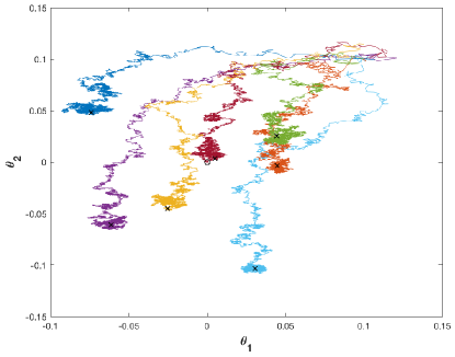
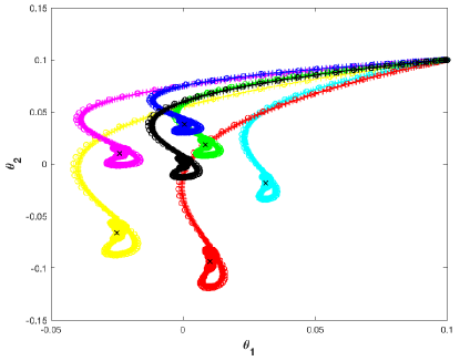
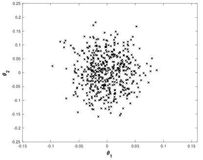
Refer to caption
Refer to caption
Refer to caption
Refer to caption
Figure 1: The scatter plot of the estimator θ^nsubscript^𝜃𝑛\hat{\theta}_{n} and the plots of sample paths for accelerated and stochastic gradient descent algorithms and their corresponding ordinary or stochastic differential equations, where δ=0.05𝛿0.05\delta=0.05, n=1000𝑛1000n=1000, m=200𝑚200m=200, initial values x0=x0n=x0m=(0.1,0.1)subscript𝑥0subscriptsuperscript𝑥𝑛0subscriptsuperscript𝑥𝑚0superscript0.10.1x_{0}=x^{n}_{0}=x^{m}_{0}=(0.1,0.1)^{\prime}, and τ=1𝜏1\tau=1. The top panels are sample paths of the gradient descent algorithms to compute θ^nsubscript^𝜃𝑛\hat{\theta}_{n}, with the top left and right panels for the stochastic gradient descent case, and the accelerated gradient descent case based on all data, respectively. In both top panels, ×\times denotes the estimator θ^nsubscript^𝜃𝑛\hat{\theta}_{n} which is the solution of the stochastic sample optimization (3.7), with \circ for the true parameter value θˇ=(0,0)ˇ𝜃00\check{\theta}=(0,0) which is the solution of the deterministic population optimization (2.1); in the top left panel, color curves are different sample paths of stochastic gradient descent; and in the top right panel, color curves with ++ and \circ correspond to sample paths of the algorithm (3.10) and their corresponding differential equation (3.11), respectively, for accelerated gradient descent based on all data, with the black curve for sample paths of the algorithm (2.4) and the ordinary differential equation (2.6). The bottom left panel is the scatter plot of 500500500 simulated θ^nsubscript^𝜃𝑛\hat{\theta}_{n}, and the bottom right panel is the marginal quantiles for V(t)𝑉𝑡V(t) (the curve with \bullet) and the corresponding estimated quantiles for Vδm(t)subscriptsuperscript𝑉𝑚𝛿𝑡V^{m}_{\delta}(t) (the curve with \circ) based on 500500500 repetitions.

Acknowledgements

The research of Yazhen Wang was supported in part by NSF grants DMS-1528375, DMS-1707605, and DMS-1913149. The authors thank action editor Ryan Tibshirani, an associate editor and three referees for helpful comments and suggestions which led to improvements of the paper.

REFERENCES

A. Ali, Z. Kolter, and R. Tibshirani. A continuous-time view of early stopping for least squares regression. International Conference on Artificial Intelligence and Statistics, 2019.

L. Ambrosio, N. Gigli, and G. Savaré. Gradient Flows: In Metric Spaces and in the Space of Probability Measures. Birkhäuser. Second edition. 2008.

Y. Arjevani, S. Shalev-Shwartz, and O. Shamir. On lower and upper bounds for smooth and strongly convex optimization problems. ArXiv preprint arXiv:1503.06833, 2015.

H. Attouch, J. Peypouquet, and P. Redont. On the fast convergence of an inertial gradient-like system with vanishing viscosity. ArXiv preprint arXiv:1507.04782, 2015.

P. Billingsley. Convergence of Probability Measures. Wiley, 2nd Edition. 1999.

P. J. Bickel, F. Götze, and W. R. van Zwet. Resampling fewer than n observations: Gains, loses, and remedies for loses. Statistica Sinica 7, 1-31. 1997.

S. Blanes, F. Casas, J. A. Oteo, and J. Ros. The Magnus expansion and some of its applications. Physics Reports 470, 151-238, 2009.

M. Bogdan, E. V. D. Berg, C. Sabatti, W. Su, and E. J. Candés. SLOPE adaptive variable selection via convex optimization. Annals of Applied Statistics, 9(3):1103-1140, 2015.

L. Bottou. Online learning and stochastic approximations. On-line learning in neural networks, 17(9):142, 1998.

S. Boyd and L. Vandenberghe. Convex Optimization. Cambridge University Press, 2004.

S. Boyd, N. Parikh, E. Chu, B. Peleato, and J. Eckstein. Distributed optimization and statistical learning via the alternating direction method of multipliers. Foundations and Trends in Machine Learning, 3(1):1-122, 2011.

A. A. Brown and M. C. Bartholomew-Biggs. Some effective methods for unconstrained optimization based on the solution of systems of ordinary differential equations. Journal of Optimization Theory and Applications, 62(2):211-224, 1989.

S. Bubeck, Y. T. Lee, and M. Singh. A geometric alternative to Nesterov’s accelerated gradient descent. ArXiv preprint arXiv:1506.08187, 2015.

S. Bubeck and N. Cesa-Bianchi. Regret analysis of stochastic and nonstochastic multi-armed bandit problems. Foundations and Trends in Machine Learning, 5(1):1-122, 2012.

J. C. Butcher. Numerical Methods for Ordinary Differential Equations. John Wiley. 2008.

V. Chandrasekarana and M. I. Jordan. Computational and statistical tradeoffs via convex relaxation. PNAS 110, no. 13, E1181-E1190. 2012.

C. Chen, D. Carlson, Z. Gan, C. Li, and L. Carin. Bridging the gap between stochastic gradient MCMC and stochastic optimization. arXiv:1512.07962v3, 2016.

C. Chen, N. Ding, and L. Carin. On the convergence of stochastic gradient MCMC algorithms with high-order integrators. arXiv:1610.06665v1, 2016.

X. Chen, J. D. Lee, X. T. Tong, Y. Zhang. Statistical inference for model parameters in stochastic gradient descent. arXiv:1610.08637, 2018.

Y. S. Chow and H. Teicher. Probability Theory. Independence, Interchangeability, Martingales. Third edition. New York, Springer. 1997.

M. Csörgö, L. Horváth, and P. Kokoszka. Approximation for bootstrapped empirical processes. Proceedings of the American Mathematical Society 128, 2457-2464. 1999.

S. Csörgö, and D. M. Mason. Bootstrapping empirical functions. Ann. Statist. 17, 1447-1471. 1989.

G. Da Prato and J. Zabczyk. Ergodicity for Infinite Dimensional Systems. Cambridge University Press, Cambridge; 1996.

A. S. Dalalyan. Further and stronger analogy between sampling and optimization: Langevin Monte Carlo and gradient descent. Proceedings of Machine Learning Research, 65:1-12, 2017.

J. Fan, W. Gong, C. J. Li, and Q. Sun. Statistical sparse online regression: A diffusion approximation perspective. Proceedings of the Twenty-First International Conference on Artificial Intelligence and Statistics, PMLR 84, 1017-1026 (2018).

N. Flammarion and F. R. Bach. From averaging to acceleration, there is only a step-size. In Proceedings of the 28th Conference on Learning Theory (COLT), 2015.

D. J. Foster, A. Sekhari, O. Shamir, N. Srebro, K. Sridharan, B. Woodworth. The complexity of making the gradient small in stochastic convex optimization. Proceedings of Machine Learning Research 99, 1-27 (2019).

A. Frieze, M. Jerrum, and R. Kannan. Learning linear transformations. FOCS 1996.

C. W. Gardiner. Stochastic Methods: A Handbook for the Natural and Social Sciences. Springer, 4th edition. 2009.

R. Ge, F. Huang, C. Jin, and Y. Yuan. Escaping from saddle points - online stochastic gradient for tensor decomposition. In COLT, 2015.

S. Ghadimi and G. Lan. Accelerated gradient methods for nonconvex nonlinear and stochastic programming. Mathematical Programming, 156(1):59-99, 2015.

I. Goodfellow, Y. Bengio, and A. Courville. Deep Learning. MIT press. 2016.

T. Hida and S. Si. Lectures on White Noise Functionals. World Scientific. 2008.

S. W. He, J. G. Wang, and J. A. Yan. Semimartingale Theory and Stochastic Calculus. Science Press and CRC Press. 1992.

C. Hu, J. T. Kwok, and W. Pan. Accelerated gradient methods for stochastic optimization and online learning. In Advances in Neural Information Processing Systems 22, 2009.

N. Ikeda and S. Watanabe. Stochastic Differential Equations and Diffusion Processes, Volume 24 (North-Holland Mathematical Library). 1981.

J. Jacod and A. Shiryaev. Limit Theorems for Stochastic Processes. Springer, 2nd edition, 2003.

S. Jastrzȩbski, Z. Kenton, D. Arpit, N. Ballas, A. Fischer, Y. Bengio, and A. Storkey. Three factors influencing minima in SGD. arXiv:1711.04623v3. 2018.

S. Ji and J.Ye. An accelerated gradient method for trace norm minimization. In Proceedings of the 26th International Conference on Machine Learning (ICML), 2009.

C. Jin, R. Ge, P. Netrapalli, S. M. Kakade, M. I. Jordan. How to escape saddle points efficiently. arXiv:1703.00887v1, 2017.

V. Jojic, S. Gould, and D. Koller. Accelerated dual decomposition for MAP inference. In Proceedings of the 27th International Conference on Machine Learning (ICML), 2010.

A. Juditsky. Convex Optimization II: Algorithms. Lecture Notes, 2013.

A. Juditsky, A. Nemirovski, and C. Tauvel. Solving variational inequalities with stochastic mirror-prox algorithm. Stoch. Syst., 1(1):17-58, 2011.

K. Kawaguchi. Deep learning without poor local minima. In Advances In Neural Information Processing Systems, pages 586-594, 2016.

N. S. Keskar, D. Mudigere, J. Nocedal, M. Smelyanskiy, and P. T. P. Tang. On Large-Batch Training for Deep Learning: Generalization Gap and Sharp Minima. arXiv:1609.04836v2, 2017.

Y. Kifer. The exit problem for small random perturbations of dynamical systems with a hyperbolic fixed point. Israel Journal of Mathematics 40, 74-96 (1981).

J. Kim and D. Pollard (1990). Cube root asymptotics. Ann. Statist.18, 191-219.

J. Komlós, P. Major, and G. Tusnády. An approximation of partial sums of independent R.V.’s and the sample DF. I. Z. Wahrschein. Verw. Gebiete 32, 111-131. 1975.

J. Komlós, P. Major, and G. Tusnády. An approximation of partial sums of independent R.V.’s and the sample DF. II. Z. Wahrschein. Verw. Gebiete 34, 33-58. 1976.

W. Krichene, A. Bayen, and P. Bartlett. Accelerated mirror descent in continuous and discrete time. In Advances in Neural Information Processing Systems (NIPS) 29, 2015.

W. Krichene, S. Krichene, and A. Bayen. Efficient Bregman projections onto the simplex. In 54th IEEE Conference on Decision and Control, 2015.

H. Kushner and G. Yin. Stochastic Approximation and Recursive Algorithms and Applications. Springer, 2003.

G. Lan. An optimal method for stochastic composite optimization. Mathematical Programming, 133(1-2):365-397, 2012.

G. Lan, Z. Lu, and R. Monteiro. Primal-dual first-order methods with O(1/ϵ)𝑂1italic-ϵO(1/\epsilon) iteration-complexity for cone programming. Mathematical Programming, 126(1):1-29, 2011.

J. D. Lee, M. Simchowitz, M. I Jordan, and B. Recht. Gradient descent only converges to minimizers. In Conference on Learning Theory, pages 1246-1257, 2016.

L. Lessard, B. Recht, and A. Packard. Analysis and design of optimization algorithms via integral quadratic constraints. SIAM Journal on Optimization, 26(1):57-95, 2016.

T. Li, L. Liu, A. Kyrillidis, and C. Caramanis. Statistical Inference Using SGD. The Thirty-Second AAAI Conference on Artificial Intelligence (AAAI-18), 3571-3578, 2018.

C. J. Li, Z. Wang, H. Liu. Online ICA: Understanding global dynamics of nonconvex optimization via diffusion processes. 30th Conference on Neural Information Processing Systems (NIPS 2016), Barcelona, Spain.

C. J. Li, M. Wang, H. Liu, and T. Zhang. Diffusion approximations for online principal component estimation and global convergence. 31th Conference on Neural Information Processing Systems (NIPS 2017), Long Beach, CA, USA. 2017a.

C. J. Li, L. Li, J. Qian, J. Liu. Batch Size Matters: A Diffusion Approximation Framework on Nonconvex Stochastic Gradient Descent. arXiv:1705.07562v2, 2017b.

H. Li and Z. Lin. Accelerated proximal gradient methods for nonconvex programming. In Advances in Neural Information Processing Systems (NIPS) 28, 2015.

Q. Li, C. Tai, W. E. Stochastic modified equations and adaptive stochastic gradient algorithms. arXiv:1511.06251v3, 2015.

Y. A. Ma, N. S. Chatterji, X. Cheng, N. Flammarion, P. L. Bartlett, c, and M. I. Jordan Is there an analog of Nesterov acceleration for MCMC? arXiv:1902.00996v1. 2019.

S. Mandt, M. D. Hoffman, and D. M. Blei. A variational analysis of stochastic gradient algorithms. arXiv:1602.02666v1, 2016.

S. Mandt, M. D. Hoffman, and D. M. Blei. Stochastic gradient descent as approximate Bayesian inference. Journal of Machine Learning Research 18, 1-35, 2017.

P. Massart. Strong Approximation for Multivariate Empirical and Related Processes, Via KMT Constructions. Ann. Probab. 17, 266-291, 1989.

Q. Meng, W. Chen, J. Yu,T. Wang, Z. Ma, T. Liu. Asynchronous Accelerated Stochastic Gradient Descent. Proceedings of the Twenty-Fifth International Joint Conference on Artificial Intelligence ((IJCAI-16). 2016.

R. Monteiro, C. Ortiz, and B. Svaiter. An adaptive accelerated first-order method for convex optimization. Technical report, ISyE, Gatech, 2012.

A. Nemirovskii and D. Yudin. Problem Complexity and Method Efficiency in Optimization. John Wiley & Sons, 1983.

Y. Nesterov. A method of solving a convex programming problem with convergence rate O(1/k2)𝑂1superscript𝑘2O(1/k^{2}). Soviet Mathematics Doklady, 27(2):372-376, 1983.

Y. Nesterov. Introductory Lectures on Convex Optimization: A Basic Course. Applied Optimization. Kluwer, 2004.

Y. Nesterov. Smooth minimization of non-smooth functions. Mathematical Programming, 103(1):127-152, 2005.

Y. Nesterov. Accelerating the cubic regularization of Newton’s method on convex problems. Mathematical Programming, 112(1):159-181, 2008.

Y. Nesterov. Gradient methods for minimizing composite functions. Mathematical Programming, 140(1):125-161, 2013.

Y. Nesterov and Boris T. Polyak. Cubic regularization of Newton’s method and its global performance. Mathematical Programming, 108(1):177-205, 2006.

J. Nocedal and S. Wright. Numerical Optimization. Springer Science & Business Media, 2006.

B. O’Donoghue and E. Candés. Adaptive restart for accelerated gradient schemes. Foundations of Computational Mathematics, 15(3):715-732, 2015.

B. O’Donoghue and E. J. Candés. Adaptive restart for accelerated gradient schemes. Found. Comput. Math., 2013.

D. Pollard. Empirical Processes: Theory and Applications. CMS. 1988.

B. T. Polyak. Introduction to optimization. Optimization Software New York, 1987.

B. T. Polyak and A. B. Juditsky. Acceleration of stochastic approximation by averaging. SIAM Journal on Control and Optimization 30 (4): 838, 1992.

M. Raginsky and J. Bouvrie. Continuous-time stochastic mirror descent on a network: Variance reduction, consensus, convergence. In CDC 2012, pages 6793-6800, 2012.

A. Rakhlin, O. Shamir, and K. Sridharan. Making Gradient Descent Optimal for Strongly Convex Stochastic Optimization. arXiv:1109.5647v7, 2012.

E. Rio. Strong Approximation for Set-Indexed Partial Sum Processes Via KMT Constructions I. Ann. Probab. 21, 759-790 (1993a).

E. Rio. Strong Approximation for Set-Indexed Partial-Sum Processes, Via KMT Constructions II. Ann. Probab. 21, 1706-1727 (1993b).

R. T. Rockafellar. Convex Analysis. Princeton Landmarks in Mathematics. Princeton University Press, 1997. Reprint of the 1970 original.

S. Ruder. An overview of gradient descent optimization algorithms. arXiv:1609.04747v1, 2016.

D. Ruppert. Efficient estimators from a slowly converging Robbins-Monro process. Technical report, 1988.

A. P. Ruszczyński. Nonlinear Optimization. Princeton University Press, 2006.

C. J. Shallue, J. Lee, J. Antognini, J. Sohl-Dickstein, R. Frostig, and G. E. Dahl. Measuring the effects of Data Parallelism on Neural Network Training. Journal of Machine Learning Research 20, 1-49 (2019).

N. Z. Shor. Minimization Methods for Non-Differentiable Functions. Springer Science & Business Media, 2012.

J. Sirignano and K. Spiliopoulos. Stochastic gradient descent in continuous time. arXiv:1611.05545v3, 2017.

J. Sirignano and K. Spiliopoulos. Stochastic gradient descent in continuous time: A central limit theorem. arXiv:1710.04273v2, 2017.

I. Sutskever, J. Martens, G. Dahl, and G. Hinton. On the importance of initialization and momentum in deep learning. In Proceedings of the 30th International Conference on Machine Learning, pages 1139-1147, 2013.

W. Su, S. Boyd, and E. J. Candés. A differential equation for modeling Nesterov’s accelerated gradient method: Theory and insights. In Advances in Neural Information Processing Systems (NIPS) 27, 2014.

Weijie Su, Stephen Boyd, and Emmanuel J. Candés. A differential equation for modeling Nesterov’s accelerated gradient method: Theory and Insights. Journal of Machine Learning Research 17, 1-43. 2016.

P. Tseng. On accelerated proximal gradient methods for convex-concave optimization. SIAM Journal on Optimization, 2008.

P. Tseng. Approximation accuracy, gradient methods, and error bound for structured convex optimization. Mathematical Programming, 125(2):263-295, 2010.

P. Toulis and E. M. Airoldi. Asymptotic and finite-sample properties of estimators based on stochastic gradients. Ann. Statist. 45(4), 1694-1727 (2017).

A. W. van der Vaart and J. Wellner. Weak Convergence and Empirical Processes With Applications to Statistics. Springer. 2000.

G. N. Watson. A Treatise on the Theory of Bessel Functions. Cambridge Mathematical Library. Cambridge University Press, 1995. Reprint of the second (1944) edition.

A. Wibisono, A. Wilson, and M. Jordan. A variational perspective on accelerated methods in optimization. Proc Natl Acad Sci 113, E7351-E7358. 2016.

Z. A. Zhu. Katyusha: The first direct acceleration of stochastic gradient methods. Journal of Machine Learning Research 18, 1-51 (2018).

Z. Zhu, J. Wu, B. Yu, L. Wu, and J. Ma The anisotropic noise in stochastic gradient descent: Its behavior of escaping from sharp minima and regularization effects. Xiv:1803.00195v5, 2019.

6 Appendix: Proofs

Denote by C𝐶C generic constant free of (δ,m,n)𝛿𝑚𝑛(\delta,m,n) whose value may change from appearance to appearance. For simplicity we take initial values x0n=x0m=x0subscriptsuperscript𝑥𝑛0subscriptsuperscript𝑥𝑚0subscript𝑥0x^{n}_{0}=x^{m}_{0}=x_{0}. In appendix sections of theorem proofs, lemmas are established under the conditions and assumptions in corresponding theorems, and we often do not repeatedly list these conditions and assumptions in the lemmas. To track processes under different circumstances and facilitate long technical arguments we adopt the following notations and conventions.

It is often necessary to put processes and random variables on some common probability spaces. At such occasions, we often automatically change probability spaces and consider versions of the processes and the random variables on new probability spaces, without altering notations. Because of this convention and Skorokhod’s representation theorem, we often switch between “convergence in probability” and “convergence in distribution.” Also because of the convention, when no confusion occurs, we try to use the same notation for random variables or processes with identical distribution.

Convention 1. We reserve x𝑥x’s and y𝑦y’s for sequences generated from gradient descent algorithms and the corresponding empirical processes, X𝑋X’s for solutions of ordinary differential equations (ODEs) and stochastic differential equations (SDEs).

Convention 2. As described at the end of Section 1, for gradient descent algorithms to solve optimization (3.7), we add superscripts n𝑛n and m𝑚m to notations for the associated processes and sequences based on all data in Section 3 and based on mini-batches in Section 4, respectively, while notations without any superscript are for sequences and functions corresponding to the optimization (2.1).

Convention 3. We reserve V𝑉V’s for normalized solutions difference between differential equations associated with the optimization (2.1) and the optimization (3.7) under the cases for all data and mini-batches, while we reserve V𝑉V without any superscript as their corresponding weak convergence limits.

Convention 4. As described at the end of Section 1, we add a superscript * to notations U𝑈U’s associated with mini-batches and as in Convention 2, their corresponding process notations have a superscript m𝑚m.

Convention 5. We denote by |Ψ|Ψ|\Psi| the absolute value of scalar ΨΨ\Psi, the Euclidean norm of vector ΨΨ\Psi, or the spectral norm of matrix ΨΨ\Psi.

6.1 Proofs of Theorem 3.1

We show that the solution of the linear differential equations (3.12) and (3.13) are Gaussian, assuming the existence and uniqueness. For the equation (3.12) its solution has an expression V(t)=Π0(t)0t[Π0(s)]1𝐙(X(s))𝑑s𝑉𝑡subscriptΠ0𝑡superscriptsubscript0𝑡superscriptdelimited-[]subscriptΠ0𝑠1𝐙𝑋𝑠differential-d𝑠V(t)=\Pi_{0}(t)\int_{0}^{t}[\Pi_{0}(s)]^{-1}{\bf Z}(X(s))ds, where Π0(t)subscriptΠ0𝑡\Pi_{0}(t) is a p𝑝p by p𝑝p deterministic matrix constructed by the Magnus expansion for solving the homogeneous linear differential equation V˙(t)+[𝑰𝑯g(X(t))]V(t)=0˙𝑉𝑡delimited-[]𝑰𝑯𝑔𝑋𝑡𝑉𝑡0\dot{V}(t)+[\boldsymbol{I\!\!H}\!g(X(t))]V(t)=0 (see Blanes et al. (2009)). Thus the limiting distribution of Vn(t)superscript𝑉𝑛𝑡V^{n}(t) is Gaussian. For the equation (3.13) in the accelerated case we may convert the second-order homogeneous linear differential equation V¨(t)+3tV˙(t)+[𝑰𝑯g(X(t))]V(t)=0¨𝑉𝑡3𝑡˙𝑉𝑡delimited-[]𝑰𝑯𝑔𝑋𝑡𝑉𝑡0\ddot{V}(t)+\frac{3}{t}\dot{V}(t)+[\boldsymbol{I\!\!H}\!g(X(t))]V(t)=0 into an equivalent first-order homogeneous linear differential equation system

(V˙(t)Ξ˙(t))=[01𝑰𝑯g(X(t))3t](V(t)Ξ(t)),˙𝑉𝑡˙Ξ𝑡delimited-[]matrix01𝑰𝑯𝑔𝑋𝑡3𝑡𝑉𝑡Ξ𝑡\left(\begin{array}[]{c}\dot{V}(t)\\ \dot{\Xi}(t)\end{array}\right)=\left[\begin{matrix}0&1\\ -\boldsymbol{I\!\!H}\!g(X(t))&-\frac{3}{t}\end{matrix}\right]\left(\begin{array}[]{c}V(t)\\ \Xi(t)\end{array}\right),

where Ξ(t)=V˙(t)Ξ𝑡˙𝑉𝑡\Xi(t)=\dot{V}(t). Similar to the first order case, we apply the Magnus expansion to solve the first-order homogeneous linear differential equation system and then show that the solution of the differential equation (3.13) linearly depends on Z()𝑍Z(\cdot). Therefore, the limiting distribution of Vn(t)superscript𝑉𝑛𝑡V^{n}(t) is also Gaussian. As a matter of fact, the theorem shows that in the special case of 𝐙(θ)=σ(θ)𝐙𝐙𝜃𝜎𝜃𝐙{\bf Z}(\theta)=\sigma(\theta){\bf Z}, we have V(t)=Π(t)𝐙𝑉𝑡Π𝑡𝐙V(t)=\Pi(t){\bf Z} to clearly indicates the Gaussian limiting distribution.

Now we are ready to provide detailed arguments for the accelerated case, as results for the plain case are relatively easier to show and will be established later. From now on for simplicity we provide proof arguments only for the case of 𝐙(θ)=𝝈(θ)𝐙𝐙𝜃𝝈𝜃𝐙{\bf Z}(\theta)=\mbox{\boldmath$\sigma$}(\theta){\bf Z}, as the proof for general 𝐙(θ)𝐙𝜃{\bf Z}(\theta) is essentially the same.

6.1.1 Differential equation derivation

With 𝐔n=(U1,,Un)τsubscript𝐔𝑛superscriptsubscript𝑈1subscript𝑈𝑛𝜏{\bf U}_{n}=(U_{1},\cdots,U_{n})^{\tau}, let Rn(θ;𝐔n)=(R1n(θ;𝐔),,Rpn(θ;𝐔n))τsuperscript𝑅𝑛𝜃subscript𝐔𝑛superscriptsubscriptsuperscript𝑅𝑛1𝜃𝐔subscriptsuperscript𝑅𝑛𝑝𝜃subscript𝐔𝑛𝜏R^{n}(\theta;{\bf U}_{n})=(R^{n}_{1}(\theta;{\bf U}),\cdots,R^{n}_{p}(\theta;{\bf U}_{n}))^{\tau}, where

Rjn(θ;𝐔n)=n[1ni=1nθj(θ;Ui)θjg(θ)],j=1,,p.formulae-sequencesuperscriptsubscript𝑅𝑗𝑛𝜃subscript𝐔𝑛𝑛delimited-[]1𝑛superscriptsubscript𝑖1𝑛subscript𝜃𝑗𝜃subscript𝑈𝑖subscript𝜃𝑗𝑔𝜃𝑗1𝑝R_{j}^{n}(\theta;{\bf U}_{n})=\sqrt{n}\left[\frac{1}{n}\sum_{i=1}^{n}\frac{\partial}{\partial\theta_{j}}\ell(\theta;U_{i})-\frac{\partial}{\partial\theta_{j}}g(\theta)\right],\qquad j=1,\cdots,p.

Then

Rn(θ;𝐔n)=n[1ni=1n(θ;Ui)g(θ)].superscript𝑅𝑛𝜃subscript𝐔𝑛𝑛delimited-[]1𝑛superscriptsubscript𝑖1𝑛𝜃subscript𝑈𝑖𝑔𝜃R^{n}(\theta;{\bf U}_{n})=\sqrt{n}\left[\frac{1}{n}\sum_{i=1}^{n}\nabla\!\ell(\theta;U_{i})-\nabla\!g(\theta)\right].

For the accelerated case, we can re-express ODE (3.11) as

X¨n(t)+3tX˙n(t)+g(Xn(t))+1nRn(Xn(t);𝐔n)=0.superscript¨𝑋𝑛𝑡3𝑡superscript˙𝑋𝑛𝑡𝑔superscript𝑋𝑛𝑡1𝑛superscript𝑅𝑛superscript𝑋𝑛𝑡subscript𝐔𝑛0\ddot{X}^{n}(t)+\frac{3}{t}\dot{X}^{n}(t)+\nabla\!g(X^{n}(t))+\frac{1}{\sqrt{n}}R^{n}(X^{n}(t);{\bf U}_{n})=0. (6.49)

By Lemma 6.5 below we obtain that Xn(t)superscript𝑋𝑛𝑡X^{n}(t) converges in probability to X(t)𝑋𝑡X(t) uniformly over any finite interval. Thus, for large n𝑛n, Xn(t)superscript𝑋𝑛𝑡X^{n}(t) falls into ΘXsubscriptΘ𝑋\Theta_{X}, and Assumption A4 implies that as n𝑛n\rightarrow\infty, Rn(Xn(t);𝐔n)=OP(1)superscript𝑅𝑛superscript𝑋𝑛𝑡subscript𝐔𝑛subscript𝑂𝑃1R^{n}(X^{n}(t);{\bf U}_{n})=O_{P}(1), and n1/2Rn(Xn(t);𝐔n)|0n^{-1/2}R^{n}(X^{n}(t);{\bf U}_{n})|\rightarrow 0. Hence, ODEs (3.11) and (6.49) both converge to ODE (2.6).

From Assumption A4 we have that Rn(θ;𝐔n)superscript𝑅𝑛𝜃subscript𝐔𝑛R^{n}(\theta;{\bf U}_{n}) converges in distribution to 𝝈(θ)𝐙𝝈𝜃𝐙\mbox{\boldmath$\sigma$}(\theta){\bf Z} uniformly over θΘX𝜃subscriptΘ𝑋\theta\in\Theta_{X}, and the generalization of Skorohod’s representation theorem in Lemma 6.1 below shows that there exist 𝐔nsuperscriptsubscript𝐔𝑛{\bf U}_{n}^{\dagger} and 𝐙subscript𝐙{\bf Z}_{\dagger} defined on some common probability spaces with 𝐙Np(0,𝐈p)similar-tosubscript𝐙subscript𝑁𝑝0subscript𝐈𝑝{\bf Z}_{\dagger}\sim N_{p}(0,{\bf I}_{p}) and 𝐔nsuperscriptsubscript𝐔𝑛{\bf U}_{n}^{\dagger} identically distributed as 𝐔nsubscript𝐔𝑛{\bf U}_{n} such that as n𝑛n\rightarrow\infty, Rn(θ;𝐔n)𝝈(θ)𝐙=o(1)superscript𝑅𝑛𝜃superscriptsubscript𝐔𝑛𝝈𝜃subscript𝐙𝑜1R^{n}(\theta;{\bf U}_{n}^{\dagger})-\mbox{\boldmath$\sigma$}(\theta){\bf Z}_{\dagger}=o(1) uniformly over θΘX𝜃subscriptΘ𝑋\theta\in\Theta_{X}. Thus we have that the solution Xn(t)superscript𝑋𝑛𝑡X^{n}(t) of equations (3.11) is identically distributed as the solution Xn(t)subscriptsuperscript𝑋𝑛𝑡X^{n}_{\dagger}(t) of

X¨n(t)+3tX˙n(t)+g(Xn(t))+1nRn(Xn(t);𝐔n)=0,subscriptsuperscript¨𝑋𝑛𝑡3𝑡subscriptsuperscript˙𝑋𝑛𝑡𝑔subscriptsuperscript𝑋𝑛𝑡1𝑛superscript𝑅𝑛subscriptsuperscript𝑋𝑛𝑡superscriptsubscript𝐔𝑛0\ddot{X}^{n}_{\dagger}(t)+\frac{3}{t}\dot{X}^{n}_{\dagger}(t)+\nabla\!g(X^{n}_{\dagger}(t))+\frac{1}{\sqrt{n}}R^{n}(X^{n}_{\dagger}(t);{\bf U}_{n}^{\dagger})=0,

which in turn may be written as

X¨n(t)+3tX˙n(t)+g(Xn(t))+1n𝝈(Xn(t))𝐙+o(n1/2)=0.subscriptsuperscript¨𝑋𝑛𝑡3𝑡subscriptsuperscript˙𝑋𝑛𝑡𝑔subscriptsuperscript𝑋𝑛𝑡1𝑛𝝈subscriptsuperscript𝑋𝑛𝑡subscript𝐙𝑜superscript𝑛120\ddot{X}^{n}_{\dagger}(t)+\frac{3}{t}\dot{X}^{n}_{\dagger}(t)+\nabla\!g(X^{n}_{\dagger}(t))+\frac{1}{\sqrt{n}}\mbox{\boldmath$\sigma$}(X^{n}_{\dagger}(t)){\bf Z}_{\dagger}+o\left(n^{-1/2}\right)=0. (6.50)

In particular (6.50) is equivalent to (3.17) up to the order of n1/2superscript𝑛12n^{-1/2}, which implies that as n𝑛n\rightarrow\infty, ODEs (3.11), (3.17), and (6.50) all converge to ODE (2.6), and Xn(t)subscriptsuperscript𝑋𝑛𝑡X^{n}_{\dagger}(t) almost surely converges to X(t)𝑋𝑡X(t). Since the solutions of equations (3.11), (3.17) and (6.50) are defined in the distribution sense, when there is no confusion, with a little abuse of notations we may drop index \dagger and write equation (6.50) as

X¨n(t)+3tX˙n(t)+g(Xn(t))+1n𝝈(Xn(t))𝐙+o(n1/2)=0,superscript¨𝑋𝑛𝑡3𝑡superscript˙𝑋𝑛𝑡𝑔superscript𝑋𝑛𝑡1𝑛𝝈superscript𝑋𝑛𝑡𝐙𝑜superscript𝑛120\ddot{X}^{n}(t)+\frac{3}{t}\dot{X}^{n}(t)+\nabla\!g(X^{n}(t))+\frac{1}{\sqrt{n}}\mbox{\boldmath$\sigma$}(X^{n}(t)){\bf Z}+o\left(n^{-1/2}\right)=0, (6.51)

where 𝐙𝐙{\bf Z} is a Gaussian random vector with distribution Np(0,𝐈p)subscript𝑁𝑝0subscript𝐈𝑝N_{p}(0,{\bf I}_{p}), and initial conditions Xn(0)=x0superscript𝑋𝑛0subscript𝑥0X^{n}(0)=x_{0} and X˙n(0)=0superscript˙𝑋𝑛00\dot{X}^{n}(0)=0.

The arguments for establishing Theorem 1 in Su et al. (2016) can be directly applied to establish the existence and uniqueness of the solution Xn(t)superscript𝑋𝑛𝑡X^{n}(t) to (6.49) for each n𝑛n. We can employ the same arguments with g()𝑔\nabla g(\cdot) replaced by 𝑰𝑯g(X(t))Π(t)+𝝈(X(t))𝑰𝑯𝑔𝑋𝑡Π𝑡𝝈𝑋𝑡\boldsymbol{I\!\!H}\!g(X(t))\,\Pi(t)+\mbox{\boldmath$\sigma$}(X(t)) or 𝑰𝑯g(X(t))V(t)+𝝈(X(t))𝐙𝑰𝑯𝑔𝑋𝑡𝑉𝑡𝝈𝑋𝑡𝐙\boldsymbol{I\!\!H}\!g(X(t))\,V(t)+\mbox{\boldmath$\sigma$}(X(t)){\bf Z} to show that linear differential equations (3.15) and (3.13) have unique solutions.

For the plain gradient descent case, Lemma 6.2 below shows that Xn(t)superscript𝑋𝑛𝑡X^{n}(t) converges to X(t)𝑋𝑡X(t) uniformly over any finite interval. Similarly we can establish that ODE (3.9) is asymptotically equivalent to ODE (3.16), and the standard ODE theory shows that they have unique solutions.

Now we give a generalization of Skorohod’s representation theorem. Assumption A4 indicates Rn(θ;𝐔n)superscript𝑅𝑛𝜃subscript𝐔𝑛R^{n}(\theta;{\bf U}_{n}) converges in distribution to 𝐙(θ)𝐙𝜃{\bf Z}(\theta), and Skorohod’s representation theorem allows to realize Rn(θ;𝐔n)superscript𝑅𝑛𝜃subscript𝐔𝑛R^{n}(\theta;{\bf U}_{n}) and 𝐙(θ)𝐙𝜃{\bf Z}(\theta) on some common probability spaces with almost sure convergence. The following lemma generalizes Skorohod’s representation theorem to have a joint representation of 𝐔nsubscript𝐔𝑛{\bf U}_{n} and Rn(θ;𝐔n)superscript𝑅𝑛𝜃subscript𝐔𝑛R^{n}(\theta;{\bf U}_{n}) along with almost sure convergence for Rn(θ;𝐔n)superscript𝑅𝑛𝜃subscript𝐔𝑛R^{n}(\theta;{\bf U}_{n}) and 𝐙(θ)𝐙𝜃{\bf Z}(\theta).

Lemma 6.1.

There exist 𝐔nsuperscriptsubscript𝐔𝑛{\bf U}_{n}^{\dagger} and 𝐙(θ)subscript𝐙𝜃{\bf Z}_{\dagger}(\theta) defined on some common probability spaces with 𝐙(θ)subscript𝐙𝜃{\bf Z}_{\dagger}(\theta) and 𝐔nsuperscriptsubscript𝐔𝑛{\bf U}_{n}^{\dagger} identically distributed as 𝐙(θ)𝐙𝜃{\bf Z}(\theta) and 𝐔nsubscript𝐔𝑛{\bf U}_{n}, respectively, such that as n𝑛n\rightarrow\infty, Rn(θ;𝐔n)𝐙(θ)=o(1)superscript𝑅𝑛𝜃superscriptsubscript𝐔𝑛subscript𝐙𝜃𝑜1R^{n}(\theta;{\bf U}_{n}^{\dagger})-{\bf Z}_{\dagger}(\theta)=o(1) uniformly over θΘX𝜃subscriptΘ𝑋\theta\in\Theta_{X}.

Proof. Our proof argument follows the construction proof of Skorohod’s representation theorem in Billingsley (1999, Theorem 6.7), with some delicate modifications involving joint distribution of 𝐔nsubscript𝐔𝑛{\bf U}_{n} and Rn(θ;𝐔n)superscript𝑅𝑛𝜃subscript𝐔𝑛R^{n}(\theta;{\bf U}_{n}) as well as its associated conditional distributions.

Let ΨθsubscriptΨ𝜃\Psi_{\theta} be the normal distribution of 𝐙(θ)𝐙𝜃{\bf Z}(\theta). Assume random variables 𝐔nsubscript𝐔𝑛{\bf U}_{n} are defined on probability space (Ω,,IP)Ω𝐼𝑃(\Omega,{\cal F},I\!\!P). Denote by Ψθ,nsubscriptΨ𝜃𝑛\Psi_{\theta,n} the joint distribution of 𝐔nsubscript𝐔𝑛{\bf U}_{n} and Rn(θ;𝐔n)superscript𝑅𝑛𝜃subscript𝐔𝑛R^{n}(\theta;{\bf U}_{n}), and by Ψθ,n,UsubscriptΨ𝜃𝑛𝑈\Psi_{\theta,n,U} and Ψθ,n,RsubscriptΨ𝜃𝑛𝑅\Psi_{\theta,n,R} the marginal distributions of 𝐔nsubscript𝐔𝑛{\bf U}_{n} and Rn(θ;𝐔n)superscript𝑅𝑛𝜃subscript𝐔𝑛R^{n}(\theta;{\bf U}_{n}), respectively. Let Ξ0(θ),,Ξk(θ)subscriptΞ0𝜃subscriptΞ𝑘𝜃\Xi_{0}(\theta),\cdots,\Xi_{k}(\theta) be the partition of IRp𝐼superscript𝑅𝑝I\!\!R^{p} (the support of normal distribution ΨθsubscriptΨ𝜃\Psi_{\theta}) such that (i) Ψθ(Ξ0(θ))<ϵsubscriptΨ𝜃subscriptΞ0𝜃italic-ϵ\Psi_{\theta}(\Xi_{0}(\theta))<\epsilon, (ii) the boundaries of Ξ0(θ),,Ξk(θ)subscriptΞ0𝜃subscriptΞ𝑘𝜃\Xi_{0}(\theta),\cdots,\Xi_{k}(\theta) have probability zero under ΨθsubscriptΨ𝜃\Psi_{\theta}, and (iii) the diameters of Ξ1(θ),,Ξk(θ)subscriptΞ1𝜃subscriptΞ𝑘𝜃\Xi_{1}(\theta),\cdots,\Xi_{k}(\theta) are bounded by ϵitalic-ϵ\epsilon. Here we use notation Ξi(θ)subscriptΞ𝑖𝜃\Xi_{i}(\theta) to indicate the possible dependence of the partitions on θ𝜃\theta. For r=1,2,𝑟12r=1,2,\cdots, we take ϵr=2rsubscriptitalic-ϵ𝑟superscript2𝑟\epsilon_{r}=2^{-r} and obtain partition Ξ0r(θ),,Ξkrr(θ)subscriptsuperscriptΞ𝑟0𝜃subscriptsuperscriptΞ𝑟subscript𝑘𝑟𝜃\Xi^{r}_{0}(\theta),\cdots,\Xi^{r}_{k_{r}}(\theta). Assumption A4 indicates that Rn(θ;𝐔n)superscript𝑅𝑛𝜃subscript𝐔𝑛R^{n}(\theta;{\bf U}_{n}) converges in distribution to 𝐙(θ)𝐙𝜃{\bf Z}(\theta) uniformly over θΘX𝜃subscriptΘ𝑋\theta\in\Theta_{X}, which implies that for each r𝑟r there exists an integer nrsubscriptsuperscript𝑛𝑟n^{*}_{r} (free of θ𝜃\theta) such that for nnr𝑛subscriptsuperscript𝑛𝑟n\geq n^{*}_{r},

Ψθ,n,R(Ξir(θ))(1ϵr)Ψθ(Ξir(θ)),i=1,,kr,θΘX.formulae-sequencesubscriptΨ𝜃𝑛𝑅subscriptsuperscriptΞ𝑟𝑖𝜃1subscriptitalic-ϵ𝑟subscriptΨ𝜃subscriptsuperscriptΞ𝑟𝑖𝜃formulae-sequence𝑖1subscript𝑘𝑟𝜃subscriptΘ𝑋\Psi_{\theta,n,R}\left(\Xi^{r}_{i}(\theta)\right)\geq(1-\epsilon_{r})\Psi_{\theta}\left(\Xi^{r}_{i}(\theta)\right),\qquad i=1,\cdots,k_{r},\;\theta\in\Theta_{X}.

As in Billingsley (1999, Theorem 6.7), we can always find a probability space to support a random element with any given distribution, and by passing to the appropriate large or infinite product space we can show that there exists a probability space (Ω,,IP)subscriptΩsubscript𝐼subscript𝑃(\Omega_{\dagger},{\cal F}_{\dagger},I\!\!P_{\dagger}) to support random variables ξ𝜉\xi, 𝐙(θ)subscript𝐙𝜃{\bf Z}_{\dagger}(\theta), 𝐔ˇnsubscriptˇ𝐔𝑛\check{{\bf U}}_{n}, and 𝐔n,isubscriptsuperscript𝐔𝑛𝑖{\bf U}^{\dagger}_{n,i}, and 𝚲nsubscript𝚲𝑛\mbox{\boldmath$\Lambda$}_{n}, n,i1𝑛𝑖1n,i\geq 1, all independent of each other, with the following four properties.

(i) ξ𝜉\xi follows a uniform distribution on [0,1]01[0,1].

(ii) 𝐙(θ)subscript𝐙𝜃{\bf Z}_{\dagger}(\theta) follows a normal distribution ΨθsubscriptΨ𝜃\Psi_{\theta}, and 𝐔ˇnsubscriptˇ𝐔𝑛\check{{\bf U}}_{n} has distribution Ψθ,n,UsubscriptΨ𝜃𝑛𝑈\Psi_{\theta,n,U}.

(iii) For each nrn<nr+1subscriptsuperscript𝑛𝑟𝑛subscriptsuperscript𝑛𝑟1n^{*}_{r}\leq n<n^{*}_{r+1} and for each Ξir(θ)subscriptsuperscriptΞ𝑟𝑖𝜃\Xi^{r}_{i}(\theta) with non-zero probability under ΨθsubscriptΨ𝜃\Psi_{\theta}, we take 𝐔n,isubscriptsuperscript𝐔𝑛𝑖{\bf U}^{\dagger}_{n,i} to be independent random variable on (Ω,,IP)subscriptΩsubscript𝐼subscript𝑃(\Omega_{\dagger},{\cal F}_{\dagger},I\!\!P_{\dagger}) such that 𝐔n,isubscriptsuperscript𝐔𝑛𝑖{\bf U}^{\dagger}_{n,i} and Rn(θ;𝐔n,i)superscript𝑅𝑛𝜃subscriptsuperscript𝐔𝑛𝑖R^{n}(\theta;{\bf U}^{\dagger}_{n,i}) jointly follow distribution Ψθ,n(|Ξir(θ))\Psi_{\theta,n}(\cdot|\Xi^{r}_{i}(\theta)), which denotes the joint conditional distribution of 𝐔n(ω)subscript𝐔𝑛𝜔{\bf U}_{n}(\omega) and Rn(θ;𝐔n(ω))superscript𝑅𝑛𝜃subscript𝐔𝑛𝜔R^{n}\left(\theta;{\bf U}_{n}(\omega)\right) given Rn(θ;𝐔n(ω))Ξir(θ)superscript𝑅𝑛𝜃subscript𝐔𝑛𝜔subscriptsuperscriptΞ𝑟𝑖𝜃R^{n}\left(\theta;{\bf U}_{n}(\omega)\right)\in\Xi^{r}_{i}(\theta) (the restriction of the joint distribution Ψθ,nsubscriptΨ𝜃𝑛\Psi_{\theta,n} on the set {𝐮,Rn(θ;𝐮)Ξir(θ)}𝐮superscript𝑅𝑛𝜃𝐮subscriptsuperscriptΞ𝑟𝑖𝜃\{{\bf u},R^{n}\left(\theta;{\bf u}\right)\in\Xi^{r}_{i}(\theta)\}). That is, for any Borel sets A1IRmsubscript𝐴1𝐼superscript𝑅𝑚A_{1}\subset I\!\!R^{m} and A2IRpsubscript𝐴2𝐼superscript𝑅𝑝A_{2}\subset I\!\!R^{p},

IP[𝐔n,i(ω)A1,Rn(θ;𝐔n,i(ω))A2]𝐼subscript𝑃delimited-[]formulae-sequencesubscriptsuperscript𝐔𝑛𝑖subscript𝜔subscript𝐴1superscript𝑅𝑛𝜃subscriptsuperscript𝐔𝑛𝑖subscript𝜔subscript𝐴2\displaystyle I\!\!P_{\dagger}\left[{\bf U}^{\dagger}_{n,i}(\omega_{\dagger})\in A_{1},R^{n}\left(\theta;{\bf U}^{\dagger}_{n,i}(\omega_{\dagger})\right)\in A_{2}\right]
=IP[𝐔ˇn(ω)A1,Rn(θ;𝐔ˇn(ω))A2|Rn(θ;𝐔ˇn(ω))Ξir(θ)]absent𝐼subscript𝑃delimited-[]formulae-sequencesubscriptˇ𝐔𝑛subscript𝜔subscript𝐴1superscript𝑅𝑛𝜃subscriptˇ𝐔𝑛subscript𝜔conditionalsubscript𝐴2superscript𝑅𝑛𝜃subscriptˇ𝐔𝑛subscript𝜔subscriptsuperscriptΞ𝑟𝑖𝜃\displaystyle=\left.I\!\!P_{\dagger}\left[\check{{\bf U}}_{n}(\omega_{\dagger})\in A_{1},R^{n}\left(\theta;\check{{\bf U}}_{n}(\omega_{\dagger})\right)\in A_{2}\right|R^{n}\left(\theta;\check{{\bf U}}_{n}(\omega_{\dagger})\right)\in\Xi^{r}_{i}(\theta)\right]
=IP[𝐔n(ω)A1,Rn(θ;𝐔n(ω))A2|Rn(θ;𝐔n(ω))Ξir(θ)]absent𝐼𝑃delimited-[]formulae-sequencesubscript𝐔𝑛𝜔subscript𝐴1superscript𝑅𝑛𝜃subscript𝐔𝑛𝜔conditionalsubscript𝐴2superscript𝑅𝑛𝜃subscript𝐔𝑛𝜔subscriptsuperscriptΞ𝑟𝑖𝜃\displaystyle=\left.I\!\!P\left[{\bf U}_{n}(\omega)\in A_{1},R^{n}\left(\theta;{\bf U}_{n}(\omega)\right)\in A_{2}\right|R^{n}\left(\theta;{\bf U}_{n}(\omega)\right)\in\Xi^{r}_{i}(\theta)\right]
=Ψθ,n(A1×A2|Ξir(θ)).absentsubscriptΨ𝜃𝑛conditionalsubscript𝐴1subscript𝐴2subscriptsuperscriptΞ𝑟𝑖𝜃\displaystyle=\Psi_{\theta,n}(A_{1}\times A_{2}|\Xi^{r}_{i}(\theta)).

Taking A1=IRmsubscript𝐴1𝐼superscript𝑅𝑚A_{1}=I\!\!R^{m} in above equality we obtain the marginal result for Rn(θ;𝐔n,i)superscript𝑅𝑛𝜃subscriptsuperscript𝐔𝑛𝑖R^{n}(\theta;{\bf U}^{\dagger}_{n,i}),

IP[Rn(θ;𝐔n,i(ω))A2]=IP[Rn(θ;𝐔ˇn(ω))A2|Rn(θ;𝐔ˇn(ω))Ξir(θ)]𝐼subscript𝑃delimited-[]superscript𝑅𝑛𝜃subscriptsuperscript𝐔𝑛𝑖subscript𝜔subscript𝐴2𝐼subscript𝑃delimited-[]superscript𝑅𝑛𝜃subscriptˇ𝐔𝑛subscript𝜔conditionalsubscript𝐴2superscript𝑅𝑛𝜃subscriptˇ𝐔𝑛subscript𝜔subscriptsuperscriptΞ𝑟𝑖𝜃\displaystyle I\!\!P_{\dagger}\left[R^{n}\left(\theta;{\bf U}^{\dagger}_{n,i}(\omega_{\dagger})\right)\in A_{2}\right]=\left.I\!\!P_{\dagger}\left[R^{n}\left(\theta;\check{{\bf U}}_{n}(\omega_{\dagger})\right)\in A_{2}\right|R^{n}\left(\theta;\check{{\bf U}}_{n}(\omega_{\dagger})\right)\in\Xi^{r}_{i}(\theta)\right]
=IP[Rn(θ;𝐔n(ω))A2|Rn(θ;𝐔n(ω))Ξir(θ)]=Ψθ,n,R(A2|Ξir(θ)).absent𝐼𝑃delimited-[]superscript𝑅𝑛𝜃subscript𝐔𝑛𝜔conditionalsubscript𝐴2superscript𝑅𝑛𝜃subscript𝐔𝑛𝜔subscriptsuperscriptΞ𝑟𝑖𝜃subscriptΨ𝜃𝑛𝑅conditionalsubscript𝐴2subscriptsuperscriptΞ𝑟𝑖𝜃\displaystyle=\left.I\!\!P\left[R^{n}\left(\theta;{\bf U}_{n}(\omega)\right)\in A_{2}\right|R^{n}\left(\theta;{\bf U}_{n}(\omega)\right)\in\Xi^{r}_{i}(\theta)\right]=\Psi_{\theta,n,R}\left(A_{2}|\Xi^{r}_{i}(\theta)\right).

(iv) For each nrn<nr+1subscriptsuperscript𝑛𝑟𝑛subscriptsuperscript𝑛𝑟1n^{*}_{r}\leq n<n^{*}_{r+1}, the distribution of 𝚲nsubscript𝚲𝑛\mbox{\boldmath$\Lambda$}_{n} is given by

νn(A)=ϵr1i=0krΨθ,n(A×IRp|Ξir(θ))[Ψθ,n,R(Ξir(θ))(1ϵr)Ψθ(Ξir(θ))].subscript𝜈𝑛𝐴superscriptsubscriptitalic-ϵ𝑟1superscriptsubscript𝑖0subscript𝑘𝑟subscriptΨ𝜃𝑛conditional𝐴𝐼superscript𝑅𝑝subscriptsuperscriptΞ𝑟𝑖𝜃delimited-[]subscriptΨ𝜃𝑛𝑅subscriptsuperscriptΞ𝑟𝑖𝜃1subscriptitalic-ϵ𝑟subscriptΨ𝜃subscriptsuperscriptΞ𝑟𝑖𝜃\displaystyle\nu_{n}(A)=\epsilon_{r}^{-1}\sum_{i=0}^{k_{r}}\Psi_{\theta,n}(A\times I\!\!R^{p}|\Xi^{r}_{i}(\theta))\left[\Psi_{\theta,n,R}(\Xi^{r}_{i}(\theta))-(1-\epsilon_{r})\Psi_{\theta}(\Xi^{r}_{i}(\theta))\right].

Now we define 𝐔nsuperscriptsubscript𝐔𝑛{\bf U}_{n}^{\dagger} on (Ω,,IP)subscriptΩsubscript𝐼subscript𝑃(\Omega_{\dagger},{\cal F}_{\dagger},I\!\!P_{\dagger}) as follows. For n<n1𝑛subscriptsuperscript𝑛1n<n^{*}_{1}, take 𝐔n,=𝐔ˇnsubscript𝐔𝑛subscriptˇ𝐔𝑛{\bf U}_{n,\dagger}=\check{{\bf U}}_{n}. For each nrn<nr+1subscriptsuperscript𝑛𝑟𝑛subscriptsuperscript𝑛𝑟1n^{*}_{r}\leq n<n^{*}_{r+1}, define

𝐔n=i=0kr𝐔n,i1{ξ1ϵr,𝐙(θ)Ξir(θ)}+𝚲n1{ξ>1ϵr}.superscriptsubscript𝐔𝑛superscriptsubscript𝑖0subscript𝑘𝑟subscriptsuperscript𝐔𝑛𝑖1formulae-sequence𝜉1subscriptitalic-ϵ𝑟subscript𝐙𝜃subscriptsuperscriptΞ𝑟𝑖𝜃subscript𝚲𝑛1𝜉1subscriptitalic-ϵ𝑟{\bf U}_{n}^{\dagger}=\sum_{i=0}^{k_{r}}{\bf U}^{\dagger}_{n,i}1\{\xi\leq 1-\epsilon_{r},{\bf Z}_{\dagger}(\theta)\in\Xi^{r}_{i}(\theta)\}+\mbox{\boldmath$\Lambda$}_{n}1\{\xi>1-\epsilon_{r}\}.

We derive the distribution of 𝐔nsuperscriptsubscript𝐔𝑛{\bf U}_{n}^{\dagger}. For any Borel set A1IRmsubscript𝐴1𝐼superscript𝑅𝑚A_{1}\subset I\!\!R^{m},

IP(𝐔nA1)=i=0krIP[𝐔n,iA1,𝐙(θ)Ξir(θ),ξ1ϵr]𝐼subscript𝑃superscriptsubscript𝐔𝑛subscript𝐴1superscriptsubscript𝑖0subscript𝑘𝑟𝐼subscript𝑃delimited-[]formulae-sequencesubscriptsuperscript𝐔𝑛𝑖subscript𝐴1formulae-sequencesubscript𝐙𝜃subscriptsuperscriptΞ𝑟𝑖𝜃𝜉1subscriptitalic-ϵ𝑟\displaystyle I\!\!P_{\dagger}({\bf U}_{n}^{\dagger}\in A_{1})=\sum_{i=0}^{k_{r}}I\!\!P_{\dagger}\left[{\bf U}^{\dagger}_{n,i}\in A_{1},{\bf Z}_{\dagger}(\theta)\in\Xi^{r}_{i}(\theta),\xi\leq 1-\epsilon_{r}\right]
+IP(𝚲nA1,ξ>1ϵr)𝐼subscript𝑃formulae-sequencesubscript𝚲𝑛subscript𝐴1𝜉1subscriptitalic-ϵ𝑟\displaystyle+I\!\!P_{\dagger}(\mbox{\boldmath$\Lambda$}_{n}\in A_{1},\xi>1-\epsilon_{r})
=(1ϵr)i=0krIP[𝐔n,iA1]IP[𝐙(θ)Ξir(θ)]+ϵrνn(A1)absent1subscriptitalic-ϵ𝑟superscriptsubscript𝑖0subscript𝑘𝑟𝐼subscript𝑃delimited-[]subscriptsuperscript𝐔𝑛𝑖subscript𝐴1𝐼subscript𝑃delimited-[]subscript𝐙𝜃subscriptsuperscriptΞ𝑟𝑖𝜃subscriptitalic-ϵ𝑟subscript𝜈𝑛subscript𝐴1\displaystyle=(1-\epsilon_{r})\sum_{i=0}^{k_{r}}I\!\!P_{\dagger}\left[{\bf U}^{\dagger}_{n,i}\in A_{1}\right]I\!\!P_{\dagger}\left[{\bf Z}_{\dagger}(\theta)\in\Xi^{r}_{i}(\theta)\right]+\epsilon_{r}\nu_{n}(A_{1})
=(1ϵr)i=0krΨθ,n(A1×IRp|Ξir(θ))Ψθ(Ξir(θ))+ϵrνn(A1)absent1subscriptitalic-ϵ𝑟superscriptsubscript𝑖0subscript𝑘𝑟subscriptΨ𝜃𝑛conditionalsubscript𝐴1𝐼superscript𝑅𝑝subscriptsuperscriptΞ𝑟𝑖𝜃subscriptΨ𝜃subscriptsuperscriptΞ𝑟𝑖𝜃subscriptitalic-ϵ𝑟subscript𝜈𝑛subscript𝐴1\displaystyle=(1-\epsilon_{r})\sum_{i=0}^{k_{r}}\Psi_{\theta,n}(A_{1}\times I\!\!R^{p}|\Xi^{r}_{i}(\theta))\Psi_{\theta}(\Xi^{r}_{i}(\theta))+\epsilon_{r}\nu_{n}(A_{1})
=i=0krΨθ,n(A×IRp|Ξir(θ))Ψθ,n,R(Ξir(θ))absentsuperscriptsubscript𝑖0subscript𝑘𝑟subscriptΨ𝜃𝑛conditional𝐴𝐼superscript𝑅𝑝subscriptsuperscriptΞ𝑟𝑖𝜃subscriptΨ𝜃𝑛𝑅subscriptsuperscriptΞ𝑟𝑖𝜃\displaystyle=\sum_{i=0}^{k_{r}}\Psi_{\theta,n}(A\times I\!\!R^{p}|\Xi^{r}_{i}(\theta))\Psi_{\theta,n,R}(\Xi^{r}_{i}(\theta))
=i=0krIP[𝐔nA1,Rn(θ;𝐔n(ω))Ξir(θ)]absentsuperscriptsubscript𝑖0subscript𝑘𝑟𝐼𝑃delimited-[]formulae-sequencesubscript𝐔𝑛subscript𝐴1superscript𝑅𝑛𝜃subscript𝐔𝑛𝜔subscriptsuperscriptΞ𝑟𝑖𝜃\displaystyle=\sum_{i=0}^{k_{r}}I\!\!P\left[{\bf U}_{n}\in A_{1},R^{n}\left(\theta;{\bf U}_{n}(\omega)\right)\in\Xi^{r}_{i}(\theta)\right]
=IP[𝐔nA1]=Ψθ,n,U(A1),absent𝐼𝑃delimited-[]subscript𝐔𝑛subscript𝐴1subscriptΨ𝜃𝑛𝑈subscript𝐴1\displaystyle=I\!\!P[{\bf U}_{n}\in A_{1}]=\Psi_{\theta,n,U}(A_{1}),

where the fifth equality is due to the definition of distribution νnsubscript𝜈𝑛\nu_{n} (which is a reverse construction). That is, we have shown that 𝐔nsuperscriptsubscript𝐔𝑛{\bf U}_{n}^{\dagger} is identically distributed as 𝐔nsubscript𝐔𝑛{\bf U}_{n} for all n𝑛n. Let Ωr,={ξ1ϵr,𝐙(θ)Ξ0r(θ)}subscriptΩ𝑟formulae-sequence𝜉1subscriptitalic-ϵ𝑟subscript𝐙𝜃subscriptsuperscriptΞ𝑟0𝜃\Omega_{r,\dagger}=\{\xi\leq 1-\epsilon_{r},{\bf Z}_{\dagger}(\theta)\not\in\Xi^{r}_{0}(\theta)\} and Ω=lim infrΩr,superscriptsubscriptΩsubscriptlimit-infimum𝑟subscriptΩ𝑟\Omega_{\dagger}^{*}=\liminf_{r\rightarrow\infty}\Omega_{r,\dagger}. Then IP(Ωr,)>12ϵr𝐼subscript𝑃superscriptsubscriptΩ𝑟12subscriptitalic-ϵ𝑟I\!\!P_{\dagger}(\Omega_{r,\dagger}^{*})>1-2\epsilon_{r}, and an application of the Borel-Cantelli lemma leads to IP(Ω)=1𝐼subscript𝑃superscriptsubscriptΩ1I\!\!P_{\dagger}(\Omega_{\dagger}^{*})=1. For nrn<nr+1subscriptsuperscript𝑛𝑟𝑛subscriptsuperscript𝑛𝑟1n^{*}_{r}\leq n<n^{*}_{r+1}, on set Ωr,subscriptΩ𝑟\Omega_{r,\dagger}, Rn(θ;𝐔n)superscript𝑅𝑛𝜃subscriptsuperscript𝐔𝑛R^{n}(\theta;{\bf U}^{\dagger}_{n}) and 𝐙(θ)subscript𝐙𝜃{\bf Z}_{\dagger}(\theta) fall into the same set Ξir(θ)subscriptsuperscriptΞ𝑟𝑖𝜃\Xi^{r}_{i}(\theta), whose diameter is less than ϵrsubscriptitalic-ϵ𝑟\epsilon_{r}. Thus, on ΩsuperscriptsubscriptΩ\Omega_{\dagger}^{*}, Rn(θ;𝐔n)superscript𝑅𝑛𝜃subscriptsuperscript𝐔𝑛R^{n}(\theta;{\bf U}^{\dagger}_{n}) a.s. converges to 𝐙(θ)subscript𝐙𝜃{\bf Z}_{\dagger}(\theta) uniformly over θΘX𝜃subscriptΘ𝑋\theta\in\Theta_{X}.

6.1.2 Weak convergence and tightness

To prove the weak convergence of Vn(t)subscript𝑉𝑛𝑡V_{n}(t) to V(t)𝑉𝑡V(t), we need to establish the usual finite-dimensional convergence plus uniform tightness (or stochastic equicontinuity) (see Kim and Pollard (1990, Theorem 2.3), Pollard (1988) and Van der Vaart and Wellner (2000)). We establish finite-dimensional convergence below.

For the accelerated case, taking a difference between ODEs (2.6) and (6.50), we have

[X¨n(t)X¨(t)]+3t[X˙n(t)X˙(t)]+[g(Xn(t))g(X(t))]+1n𝝈(Xn(t))𝐙=o(n1/2).delimited-[]subscriptsuperscript¨𝑋𝑛𝑡¨𝑋𝑡3𝑡delimited-[]subscriptsuperscript˙𝑋𝑛𝑡˙𝑋𝑡𝑔subscriptsuperscript𝑋𝑛𝑡𝑔𝑋𝑡1𝑛𝝈subscriptsuperscript𝑋𝑛𝑡subscript𝐙𝑜superscript𝑛12\displaystyle[\ddot{X}^{n}_{\dagger}(t)-\ddot{X}(t)]+\frac{3}{t}[\dot{X}^{n}_{\dagger}(t)-\dot{X}(t)]+\nabla\![g(X^{n}_{\dagger}(t))-g(X(t))]+\frac{1}{\sqrt{n}}\mbox{\boldmath$\sigma$}(X^{n}_{\dagger}(t)){\bf Z}_{\dagger}=o\left(n^{-1/2}\right).

Let Vn(t)=n[Xn(t)X(t)]subscriptsuperscript𝑉𝑛𝑡𝑛delimited-[]subscriptsuperscript𝑋𝑛𝑡𝑋𝑡V^{n}_{\dagger}(t)=\sqrt{n}[X^{n}_{\dagger}(t)-X(t)]. As n𝑛n\rightarrow\infty, Xn(t)a.s.X(t)subscriptformulae-sequence𝑎𝑠subscriptsuperscript𝑋𝑛𝑡𝑋𝑡X^{n}_{\dagger}(t)\rightarrow_{a.s.}X(t), 𝝈(Xn(t))=𝝈(X(t))+o(1)𝝈subscriptsuperscript𝑋𝑛𝑡𝝈𝑋𝑡𝑜1\mbox{\boldmath$\sigma$}(X^{n}_{\dagger}(t))=\mbox{\boldmath$\sigma$}(X(t))+o(1), and [g(Xn(t))g(X(t))]=2g(X(t))[Xn(t)X(t)]+o(Xn(t)X(t)),𝑔subscriptsuperscript𝑋𝑛𝑡𝑔𝑋𝑡superscript2𝑔𝑋𝑡delimited-[]subscriptsuperscript𝑋𝑛𝑡𝑋𝑡𝑜subscriptsuperscript𝑋𝑛𝑡𝑋𝑡\nabla\![g(X^{n}_{\dagger}(t))-g(X(t))]=\nabla^{2}\!g(X(t))[X^{n}_{\dagger}(t)-X(t)]+o(X^{n}_{\dagger}(t)-X(t)), thus Vn(t)subscriptsuperscript𝑉𝑛𝑡V^{n}_{\dagger}(t) satisfies

V¨n(t)+3tV˙n(t)+𝑰𝑯g(X(t))Vn(t)+𝝈(X(t))𝐙=o(1).subscriptsuperscript¨𝑉𝑛𝑡3𝑡subscriptsuperscript˙𝑉𝑛𝑡𝑰𝑯𝑔𝑋𝑡subscriptsuperscript𝑉𝑛𝑡𝝈𝑋𝑡subscript𝐙𝑜1\displaystyle\ddot{V}^{n}_{\dagger}(t)+\frac{3}{t}\dot{V}^{n}_{\dagger}(t)+\boldsymbol{I\!\!H}\!g(X(t))V^{n}_{\dagger}(t)+\mbox{\boldmath$\sigma$}(X(t)){\bf Z}_{\dagger}=o(1).

As n𝑛n\rightarrow\infty, Vn(t)subscriptsuperscript𝑉𝑛𝑡V^{n}_{\dagger}(t) almost surely converge to the unique solution V(t)subscript𝑉𝑡V_{\dagger}(t) of the following linear differential equation,

V¨(t)+3tV˙(t)+[𝑰𝑯g(X(t))]V(t)+𝝈(X(t))𝐙=0,subscript¨𝑉𝑡3𝑡subscript˙𝑉𝑡delimited-[]𝑰𝑯𝑔𝑋𝑡subscript𝑉𝑡𝝈𝑋𝑡subscript𝐙0\ddot{V}_{\dagger}(t)+\frac{3}{t}\dot{V}_{\dagger}(t)+[\boldsymbol{I\!\!H}\!g(X(t))]V_{\dagger}(t)+\mbox{\boldmath$\sigma$}(X(t)){\bf Z}_{\dagger}=0,

where X(t)𝑋𝑡X(t) is the solution of equation (2.6), random variable 𝐙Np(0,𝐈p)similar-tosubscript𝐙subscript𝑁𝑝0subscript𝐈𝑝{\bf Z}_{\dagger}\sim N_{p}(0,{\bf I}_{p}), and initial conditions V(0)=V˙(0)=0subscript𝑉0subscript˙𝑉00V_{\dagger}(0)=\dot{V}_{\dagger}(0)=0. As V(t)𝑉𝑡V(t) and V(t)subscript𝑉𝑡V_{\dagger}(t) are governed by the equations with the same form but identically distributed random coefficients 𝐙𝐙{\bf Z} and 𝐙subscript𝐙{\bf Z}_{\dagger}, we easily see that V(t)𝑉𝑡V(t) and V(t)subscript𝑉𝑡V_{\dagger}(t) are identically distributed.

The almost sure convergence of Vn(t)subscriptsuperscript𝑉𝑛𝑡V^{n}_{\dagger}(t) to V(t)subscript𝑉𝑡V_{\dagger}(t) implies the joint convergence of (Vn(t1),,Vn(tk))subscriptsuperscript𝑉𝑛subscript𝑡1subscriptsuperscript𝑉𝑛subscript𝑡𝑘(V^{n}_{\dagger}(t_{1}),\cdots,V^{n}_{\dagger}(t_{k})) to (V(t1),,V(tk))subscript𝑉subscript𝑡1subscript𝑉subscript𝑡𝑘(V_{\dagger}(t_{1}),\cdots,V_{\dagger}(t_{k})) for any integer k𝑘k and any t1,,tkIR+subscript𝑡1subscript𝑡𝑘𝐼subscript𝑅t_{1},\cdots,t_{k}\in I\!\!R_{+}. From the identical distributions of Xn(t)superscript𝑋𝑛𝑡X^{n}(t) with Xn(t)subscriptsuperscript𝑋𝑛𝑡X^{n}_{\dagger}(t), Vn(t)superscript𝑉𝑛𝑡V^{n}(t) with Vn(t)subscriptsuperscript𝑉𝑛𝑡V^{n}_{\dagger}(t), and V(t)𝑉𝑡V(t) with V(t)subscript𝑉𝑡V_{\dagger}(t) we immediately conclude that (Vn(t1),,Vn(tk))superscript𝑉𝑛subscript𝑡1superscript𝑉𝑛subscript𝑡𝑘(V^{n}(t_{1}),\cdots,V^{n}(t_{k})) converges in distribution to (V(t1),,V(tk))𝑉subscript𝑡1𝑉subscript𝑡𝑘(V(t_{1}),\cdots,V(t_{k})). This establishes finite-dimensional distribution convergence of Vn(t)superscript𝑉𝑛𝑡V^{n}(t) to V(t)𝑉𝑡V(t).

For the plain gradient descent case, an application of the similar argument to ODEs (2.3) and (3.16) can establish finite-dimensional convergence.

Now we show tightness of Vn(t)subscript𝑉𝑛𝑡V_{n}(t). To establish the tightness of Vn(t)subscript𝑉𝑛𝑡V_{n}(t) on [0,T]0𝑇[0,T], we need to show that for any ε>0𝜀0\varepsilon>0, and η>0𝜂0\eta>0, there exists a positive constant δ𝛿\delta such that

lim supnP[sup(t1,t2)𝒯(T,δ)|Vn(t1)Vn(t2)|>η]<ε,subscriptlimit-supremum𝑛𝑃delimited-[]subscriptsupremumsubscript𝑡1subscript𝑡2𝒯𝑇𝛿subscript𝑉𝑛subscript𝑡1subscript𝑉𝑛subscript𝑡2𝜂𝜀\limsup_{n\rightarrow\infty}P\left[\sup_{(t_{1},t_{2})\in{\cal T}(T,\delta)}|V_{n}(t_{1})-V_{n}(t_{2})|>\eta\right]<\varepsilon, (6.52)

where 𝒯(T,δ)={(t1,t2),t1,t2IR+,max(t1,t2)T,|t1t2|<δ}{\cal T}(T,\delta)=\{(t_{1},t_{2}),t_{1},t_{2}\in I\!\!R_{+},\max(t_{1},t_{2})\leq T,|t_{1}-t_{2}|<\delta\}. The tightness of Vn(t)subscript𝑉𝑛𝑡V_{n}(t) on IR+𝐼subscript𝑅I\!\!R_{+} requires above result for any T<𝑇T<\infty.

Note that as (6.52) requires only some probability evaluation, with the abuse of notations we have dropped index \dagger and work on equation (6.51).

6.1.3 Weak convergence proof for the plain gradient descent case

Lemma 6.2.

For any given T>0𝑇0T>0, we have

maxt[0,T]|Xn(t)X(t)|=OP(n1/2).subscript𝑡0𝑇superscript𝑋𝑛𝑡𝑋𝑡subscript𝑂𝑃superscript𝑛12\max_{t\in[0,T]}|X^{n}(t)-X(t)|=O_{P}(n^{-1/2}).

Proof. From ODEs (2.3) and (3.9) we have

X˙n(t)X˙(t)=[g(Xn(t))g(X(t))]n1/2Rn(Xn(t);𝐔n),superscript˙𝑋𝑛𝑡˙𝑋𝑡delimited-[]𝑔superscript𝑋𝑛𝑡𝑔𝑋𝑡superscript𝑛12superscript𝑅𝑛superscript𝑋𝑛𝑡subscript𝐔𝑛\dot{X}^{n}(t)-\dot{X}(t)=-[\nabla g(X^{n}(t))-\nabla g(X(t))]-n^{-1/2}R^{n}(X^{n}(t);{\bf U}_{n}),

and using assumption A1-A2 we obtain

|g(Xn(t))g(X(t))|L|Xn(t)X(t)|,𝑔superscript𝑋𝑛𝑡𝑔𝑋𝑡𝐿superscript𝑋𝑛𝑡𝑋𝑡\displaystyle|\nabla g(X^{n}(t))-\nabla g(X(t))|\leq L|X^{n}(t)-X(t)|,
n1/2|Rn(Xn(t);𝐔n)Rn(X(t);𝐔n)|(n1i=1nh1(Ui)+L)|Xn(t)X(t)|.superscript𝑛12superscript𝑅𝑛superscript𝑋𝑛𝑡subscript𝐔𝑛superscript𝑅𝑛𝑋𝑡subscript𝐔𝑛superscript𝑛1superscriptsubscript𝑖1𝑛subscript1subscript𝑈𝑖𝐿superscript𝑋𝑛𝑡𝑋𝑡\displaystyle n^{-1/2}|R^{n}(X^{n}(t);{\bf U}_{n})-R^{n}(X(t);{\bf U}_{n})|\leq\left(n^{-1}\sum_{i=1}^{n}h_{1}(U_{i})+L\right)|X^{n}(t)-X(t)|.

Combining them together we arrive at

|Xn(t)X(t)|n1/20t|Rn(X(s);𝐔n)|𝑑s+(n1i=1nh1(Ui)+2L)0t|Xn(s)X(s)|𝑑s,superscript𝑋𝑛𝑡𝑋𝑡superscript𝑛12subscriptsuperscript𝑡0superscript𝑅𝑛𝑋𝑠subscript𝐔𝑛differential-d𝑠superscript𝑛1superscriptsubscript𝑖1𝑛subscript1subscript𝑈𝑖2𝐿superscriptsubscript0𝑡superscript𝑋𝑛𝑠𝑋𝑠differential-d𝑠\displaystyle|X^{n}(t)-X(t)|\leq n^{-1/2}\int^{t}_{0}|R^{n}(X(s);{\bf U}_{n})|ds+\left(n^{-1}\sum_{i=1}^{n}h_{1}(U_{i})+2L\right)\int_{0}^{t}|X^{n}(s)-X(s)|ds,

and an application of Gronwall’s inequality leads to

|Xn(t)X(t)|n1/20t|Rn(X(s);𝐔n)|𝑑ssuperscript𝑋𝑛𝑡𝑋𝑡superscript𝑛12subscriptsuperscript𝑡0superscript𝑅𝑛𝑋𝑠subscript𝐔𝑛differential-d𝑠\displaystyle|X^{n}(t)-X(t)|\leq n^{-1/2}\int^{t}_{0}|R^{n}(X(s);{\bf U}_{n})|ds
+n1/2(n1i=1nh1(Ui)+2L)0te(n1i=1nh1(Ui)+2L)u𝑑u0u|Rn(X(s);𝐔n)|𝑑s,superscript𝑛12superscript𝑛1superscriptsubscript𝑖1𝑛subscript1subscript𝑈𝑖2𝐿superscriptsubscript0𝑡superscript𝑒superscript𝑛1superscriptsubscript𝑖1𝑛subscript1subscript𝑈𝑖2𝐿𝑢differential-d𝑢superscriptsubscript0𝑢superscript𝑅𝑛𝑋𝑠subscript𝐔𝑛differential-d𝑠\displaystyle+n^{-1/2}\left(n^{-1}\sum_{i=1}^{n}h_{1}(U_{i})+2L\right)\int_{0}^{t}e^{\left(n^{-1}\sum_{i=1}^{n}h_{1}(U_{i})+2L\right)u}du\int_{0}^{u}|R^{n}(X(s);{\bf U}_{n})|ds,

which implies

maxt[0,T]|Xn(t)X(t)|n1/20T|Rn(X(s);𝐔n)|𝑑ssubscript𝑡0𝑇superscript𝑋𝑛𝑡𝑋𝑡superscript𝑛12subscriptsuperscript𝑇0superscript𝑅𝑛𝑋𝑠subscript𝐔𝑛differential-d𝑠\displaystyle\max_{t\in[0,T]}|X^{n}(t)-X(t)|\leq n^{-1/2}\int^{T}_{0}|R^{n}(X(s);{\bf U}_{n})|ds
+n1/2(n1i=1nh1(Ui)+2L)0Te(n1i=1nh1(Ui)+2L)u𝑑u0u|Rn(X(s);𝐔n)|𝑑s.superscript𝑛12superscript𝑛1superscriptsubscript𝑖1𝑛subscript1subscript𝑈𝑖2𝐿superscriptsubscript0𝑇superscript𝑒superscript𝑛1superscriptsubscript𝑖1𝑛subscript1subscript𝑈𝑖2𝐿𝑢differential-d𝑢superscriptsubscript0𝑢superscript𝑅𝑛𝑋𝑠subscript𝐔𝑛differential-d𝑠\displaystyle+n^{-1/2}\left(n^{-1}\sum_{i=1}^{n}h_{1}(U_{i})+2L\right)\int_{0}^{T}e^{\left(n^{-1}\sum_{i=1}^{n}h_{1}(U_{i})+2L\right)u}du\int_{0}^{u}|R^{n}(X(s);{\bf U}_{n})|ds.

Since assumptions A3 and A4 indicate supt|Rn(X(t);𝐔n)|supt|𝝈(X(t))𝐙|=OP(1)similar-tosubscriptsupremum𝑡superscript𝑅𝑛𝑋𝑡subscript𝐔𝑛subscriptsupremum𝑡𝝈𝑋𝑡𝐙subscript𝑂𝑃1\sup_{t}|R^{n}(X(t);{\bf U}_{n})|\sim\sup_{t}|\mbox{\boldmath$\sigma$}(X(t)){\bf Z}|=O_{P}(1), and n1i=1nh1(Ui)superscript𝑛1superscriptsubscript𝑖1𝑛subscript1subscript𝑈𝑖n^{-1}\sum_{i=1}^{n}h_{1}(U_{i}) converges in probability to E[h1(U)]<𝐸delimited-[]subscript1𝑈E[h_{1}(U)]<\infty, the above inequality shows maxt[0,T]|Xn(t)X(t)|=OP(n1/2)subscript𝑡0𝑇superscript𝑋𝑛𝑡𝑋𝑡subscript𝑂𝑃superscript𝑛12\max_{t\in[0,T]}|X^{n}(t)-X(t)|=O_{P}(n^{-1/2}).

Lemma 6.3.

For any given T>0𝑇0T>0, Vn(t)superscript𝑉𝑛𝑡V^{n}(t) is stochastically equicontinuous on [0,T].

Proof. Lemma 6.2 has shown maxt[0,T]|Vn(t)|=OP(1)subscript𝑡0𝑇superscript𝑉𝑛𝑡subscript𝑂𝑃1\max_{t\in[0,T]}|V^{n}(t)|=O_{P}(1). From ODEs (2.3) and (3.9) we have

V˙n(t)=n[X˙n(t)X˙(t)]=n[g(Xn(t))g(X(t))]Rn(Xn(t);𝐔n),superscript˙𝑉𝑛𝑡𝑛delimited-[]superscript˙𝑋𝑛𝑡˙𝑋𝑡𝑛delimited-[]𝑔superscript𝑋𝑛𝑡𝑔𝑋𝑡superscript𝑅𝑛superscript𝑋𝑛𝑡subscript𝐔𝑛\displaystyle\dot{V}^{n}(t)=\sqrt{n}[\dot{X}^{n}(t)-\dot{X}(t)]=-\sqrt{n}[\nabla g(X^{n}(t))-\nabla g(X(t))]-R^{n}(X^{n}(t);{\bf U}_{n}),
|V˙n(t)|n|g(Xn(t))g(X(t))|+|Rn(Xn(t);𝐔n)|superscript˙𝑉𝑛𝑡𝑛𝑔superscript𝑋𝑛𝑡𝑔𝑋𝑡superscript𝑅𝑛superscript𝑋𝑛𝑡subscript𝐔𝑛\displaystyle|\dot{V}^{n}(t)|\leq\sqrt{n}|\nabla g(X^{n}(t))-\nabla g(X(t))|+|R^{n}(X^{n}(t);{\bf U}_{n})|
Ln|Xn(t))X(t)|+|Rn(Xn(t);𝐔n)|.\displaystyle\leq L\sqrt{n}|X^{n}(t))-X(t)|+|R^{n}(X^{n}(t);{\bf U}_{n})|.

Lemma 6.2 shows that n|Xn(t))X(t)|=OP(1)\sqrt{n}|X^{n}(t))-X(t)|=O_{P}(1), which indicates that for large n𝑛n, Xn(t)superscript𝑋𝑛𝑡X^{n}(t) falls into ΘXsubscriptΘ𝑋\Theta_{X} and assumption A4 in turn implies |suptRn(Xn(t);𝐔n)|supt|𝝈(Xn(t))𝐙|=OP(1)similar-tosubscriptsupremum𝑡superscript𝑅𝑛superscript𝑋𝑛𝑡subscript𝐔𝑛subscriptsupremum𝑡𝝈superscript𝑋𝑛𝑡𝐙subscript𝑂𝑃1|\sup_{t}R^{n}(X^{n}(t);{\bf U}_{n})|\sim\sup_{t}|\mbox{\boldmath$\sigma$}(X^{n}(t)){\bf Z}|=O_{P}(1). Substituting these into the upper bound of |V˙n(t)|superscript˙𝑉𝑛𝑡|\dot{V}^{n}(t)| we prove that maxt[0,T]|V˙n(t)|=OP(1)subscript𝑡0𝑇superscript˙𝑉𝑛𝑡subscript𝑂𝑃1\max_{t\in[0,T]}|\dot{V}^{n}(t)|=O_{P}(1). Combining this with maxt[0,T]|Vn(t)|=OP(1)subscript𝑡0𝑇superscript𝑉𝑛𝑡subscript𝑂𝑃1\max_{t\in[0,T]}|V^{n}(t)|=O_{P}(1) shown in Lemma 6.2, we immediately establish the lemma.

Proof of Theorem 3.1 for the plain gradient descent case The same perturbation argument in Section 6.1.2 can be used to show finite-dimensional distribution convergence of Vn(t)superscript𝑉𝑛𝑡V^{n}(t) to V(t)𝑉𝑡V(t) for simple ODE (3.9) in the plain gradient descent case. With the tightness of Vn(t)superscript𝑉𝑛𝑡V^{n}(t) shown in Lemma 6.3 together with the finite distribution convergence we immediately prove the weak convergence of Vn(t)superscript𝑉𝑛𝑡V^{n}(t) to V(t)𝑉𝑡V(t) in the plain gradient descent case.

6.1.4 Weak Convergence proof for the accelerated case

We can use the same proof in Su et al. (2016, Theorem 1) to show that ODE (3.11) has a unique solution for each n𝑛n and 𝐔nsubscript𝐔𝑛{\bf U}_{n}. While the proof arguments in Su et al. (2016, Theorem 1) mainly require local ODE properties such as those near a neighbor of zero, our weak convergence analysis needs to investigate global behaviors of processes generated from SDEs and ODEs with random coefficients. We will first extend and refine some local results for the global case and establish several preparatory lemmas for proving weak convergence in the theorem.

Given an interval =[s,t]𝑠𝑡\mathcal{I}=[s,t] and a process Y(t)𝑌𝑡Y(t), define for a(0,1]𝑎01a\in(0,1],

Ma(s,t;Y)=Ma(;Y)=supu[s,t]|Y˙(u)Y˙(s)(us)a|.subscript𝑀𝑎𝑠𝑡𝑌subscript𝑀𝑎𝑌subscriptsupremum𝑢𝑠𝑡˙𝑌𝑢˙𝑌𝑠superscript𝑢𝑠𝑎M_{a}(s,t;Y)=M_{a}(\mathcal{I};Y)=\sup_{u\in[s,t]}\left|\frac{\dot{Y}(u)-\dot{Y}(s)}{(u-s)^{a}}\right|. (6.53)

In the proof of Theorem 3.1 we take a=1𝑎1a=1 and use M1(s,t;Y)subscript𝑀1𝑠𝑡𝑌M_{1}(s,t;Y). We will need Ma(s,t;Y)subscript𝑀𝑎𝑠𝑡𝑌M_{a}(s,t;Y) with a<1𝑎1a<1 later in the proof of Theorems 4.5.

Lemma 6.4.

For X(t)𝑋𝑡X(t) and Xn(t)superscript𝑋𝑛𝑡X^{n}(t) we have the following inequalities,

M1(s,t;X)11L(ts)2/6[(3s+L(ts)2)|X˙(s)|+|g(X(s))|],subscript𝑀1𝑠𝑡𝑋11𝐿superscript𝑡𝑠26delimited-[]3𝑠𝐿𝑡𝑠2˙𝑋𝑠𝑔𝑋𝑠\displaystyle M_{1}(s,t;X)\leq\frac{1}{1-L(t-s)^{2}/6}\left[\left(\frac{3}{s}+\frac{L(t-s)}{2}\right)|\dot{X}(s)|+|\nabla g(X(s))|\right],
M1(s,t;Xn)11[ζ(𝐔n)+2L](ts)2/6subscript𝑀1𝑠𝑡superscript𝑋𝑛11delimited-[]𝜁subscript𝐔𝑛2𝐿superscript𝑡𝑠26\displaystyle M_{1}(s,t;X^{n})\leq\frac{1}{1-[\zeta({\bf U}_{n})+2L](t-s)^{2}/6}
[(3s+[ζ(𝐔n)+2L](ts)2)|X˙n(s)|+|g(Xn(s))|+n1/2|Rn(Xn(s);𝐔n)|],delimited-[]3𝑠delimited-[]𝜁subscript𝐔𝑛2𝐿𝑡𝑠2superscript˙𝑋𝑛𝑠𝑔superscript𝑋𝑛𝑠superscript𝑛12superscript𝑅𝑛superscript𝑋𝑛𝑠subscript𝐔𝑛\displaystyle\left[\left(\frac{3}{s}+\frac{[\zeta({\bf U}_{n})+2L](t-s)}{2}\right)|\dot{X}^{n}(s)|+|\nabla g(X^{n}(s))|+n^{-1/2}|R^{n}(X^{n}(s);{\bf U}_{n})|\right],
M1(s,t;XnX)11[ζ(𝐔n)+2L](ts)2/6{(3/s+(ts)[ζ(𝐔n)+2L])|X˙n(s)X˙(s)|\displaystyle M_{1}(s,t;X^{n}-X)\leq\frac{1}{1-[\zeta({\bf U}_{n})+2L](t-s)^{2}/6}\left\{(3/s+(t-s)[\zeta({\bf U}_{n})+2L])|\dot{X}^{n}(s)-\dot{X}(s)|\right.
+[2ζ(𝐔n)+5L]|Xn(s)X(s)|+n1/2|Rn(Xn(s);𝐔n)|delimited-[]2𝜁subscript𝐔𝑛5𝐿superscript𝑋𝑛𝑠𝑋𝑠superscript𝑛12superscript𝑅𝑛superscript𝑋𝑛𝑠subscript𝐔𝑛\displaystyle+[2\zeta({\bf U}_{n})+5L]|X^{n}(s)-X(s)|+n^{-1/2}|R^{n}(X^{n}(s);{\bf U}_{n})|
+n1/2supu[s,t]|Rn(X(u);𝐔n)Rn(X(s);𝐔n)|},\displaystyle\left.+n^{-1/2}\sup_{u\in[s,t]}|R^{n}(X(u);{\bf U}_{n})-R^{n}(X(s);{\bf U}_{n})|\right\},

when s>0𝑠0s>0 and ts<6/[ζ(𝐔n)+2L]𝑡𝑠6delimited-[]𝜁subscript𝐔𝑛2𝐿t-s<\sqrt{6/[\zeta({\bf U}_{n})+2L]}, ζ(𝐔n)=1ni=1nh1(Ui)𝜁subscript𝐔𝑛1𝑛superscriptsubscript𝑖1𝑛subscript1subscript𝑈𝑖\zeta({\bf U}_{n})=\frac{1}{n}\sum_{i=1}^{n}h_{1}(U_{i}), and h1()subscript1h_{1}(\cdot) is given in assumption A1. In particular for s=0𝑠0s=0,

M1(0,t;X)|g(x0)|1Lt2/6,M1(0,t;Xn)|g(x0)|+n1/2|Rn(x0;𝐔n)|1[ζ(𝐔n)+2L]t2/6,formulae-sequencesubscript𝑀10𝑡𝑋𝑔subscript𝑥01𝐿superscript𝑡26subscript𝑀10𝑡superscript𝑋𝑛𝑔subscript𝑥0superscript𝑛12superscript𝑅𝑛subscript𝑥0subscript𝐔𝑛1delimited-[]𝜁subscript𝐔𝑛2𝐿superscript𝑡26M_{1}(0,t;X)\leq\frac{|\nabla g(x_{0})|}{1-Lt^{2}/6},\;\;M_{1}(0,t;X^{n})\leq\frac{|\nabla g(x_{0})|+n^{-1/2}|R^{n}(x_{0};{\bf U}_{n})|}{1-[\zeta({\bf U}_{n})+2L]t^{2}/6},
M1(0,t;XnX)n1/21[ζ(𝐔n)+2L]t2/6subscript𝑀10𝑡superscript𝑋𝑛𝑋superscript𝑛121delimited-[]𝜁subscript𝐔𝑛2𝐿superscript𝑡26M_{1}(0,t;X^{n}-X)\leq\frac{n^{-1/2}}{1-[\zeta({\bf U}_{n})+2L]t^{2}/6}
[|Rn(x0;𝐔n)|+supu[0,t]|Rn(X(u);𝐔n)Rn(x0;𝐔n)|].delimited-[]superscript𝑅𝑛subscript𝑥0subscript𝐔𝑛subscriptsupremum𝑢0𝑡superscript𝑅𝑛𝑋𝑢subscript𝐔𝑛superscript𝑅𝑛subscript𝑥0subscript𝐔𝑛\left[|R^{n}(x_{0};{\bf U}_{n})|+\sup_{u\in[0,t]}|R^{n}(X(u);{\bf U}_{n})-R^{n}(x_{0};{\bf U}_{n})|\right].

Proof. Because of similarity, we provide proof arguments only for M1(s,t;XnX)subscript𝑀1𝑠𝑡superscript𝑋𝑛𝑋M_{1}(s,t;X^{n}-X). As Vn(t)=n[Xn(t)X(t)]superscript𝑉𝑛𝑡𝑛delimited-[]superscript𝑋𝑛𝑡𝑋𝑡V^{n}(t)=\sqrt{n}[X^{n}(t)-X(t)], M1(s,t;Vn)=nM1(s,t;XnX)subscript𝑀1𝑠𝑡superscript𝑉𝑛𝑛subscript𝑀1𝑠𝑡superscript𝑋𝑛𝑋M_{1}(s,t;V^{n})=\sqrt{n}M_{1}(s,t;X^{n}-X), and we will establish the inequality for M1(s,t;Vn)subscript𝑀1𝑠𝑡superscript𝑉𝑛M_{1}(s,t;V^{n}). Vn(t)superscript𝑉𝑛𝑡V^{n}(t) satisfies the differential equation

V¨n(t)+3tV˙n(t)+n[g(Xn(t))g(X(t))]+Rn(Xn(t);𝐔n)=0.superscript¨𝑉𝑛𝑡3𝑡superscript˙𝑉𝑛𝑡𝑛𝑔superscript𝑋𝑛𝑡𝑔𝑋𝑡superscript𝑅𝑛superscript𝑋𝑛𝑡subscript𝐔𝑛0\ddot{V}^{n}(t)+\frac{3}{t}\dot{V}^{n}(t)+\sqrt{n}\nabla\![g(X^{n}(t))-g(X(t))]+R^{n}(X^{n}(t);{\bf U}_{n})=0. (6.54)

Let

H(t;Vn)=n[g(Xn(t))g(X(t))]+Rn(Xn(t);𝐔n),𝐻𝑡superscript𝑉𝑛𝑛𝑔superscript𝑋𝑛𝑡𝑔𝑋𝑡superscript𝑅𝑛superscript𝑋𝑛𝑡subscript𝐔𝑛\displaystyle H(t;V^{n})=\sqrt{n}\nabla\![g(X^{n}(t))-g(X(t))]+R^{n}(X^{n}(t);{\bf U}_{n}),

and J(s,t;H,Vn)=stu3[H(u;Vn)H(s;Vn)]𝑑u𝐽𝑠𝑡𝐻superscript𝑉𝑛superscriptsubscript𝑠𝑡superscript𝑢3delimited-[]𝐻𝑢superscript𝑉𝑛𝐻𝑠superscript𝑉𝑛differential-d𝑢J(s,t;H,V^{n})=\int_{s}^{t}u^{3}[H(u;V^{n})-H(s;V^{n})]du. Then

|H(t;Vn)H(s;Vn)|n|[g(Xn(t))g(Xn(s))g(X(t))+g(X(s))]|𝐻𝑡superscript𝑉𝑛𝐻𝑠superscript𝑉𝑛𝑛𝑔superscript𝑋𝑛𝑡𝑔superscript𝑋𝑛𝑠𝑔𝑋𝑡𝑔𝑋𝑠\displaystyle|H(t;V^{n})-H(s;V^{n})|\leq\sqrt{n}|\nabla[g(X^{n}(t))-g(X^{n}(s))-g(X(t))+g(X(s))]|
+|Rn(Xn(t);𝐔n)Rn(Xn(s);𝐔n)|.superscript𝑅𝑛superscript𝑋𝑛𝑡subscript𝐔𝑛superscript𝑅𝑛superscript𝑋𝑛𝑠subscript𝐔𝑛\displaystyle+|R^{n}(X^{n}(t);{\bf U}_{n})-R^{n}(X^{n}(s);{\bf U}_{n})|.

As in the proof of Lemma 6.2, using assumptions A1-A2 we obtain

n|[g(Xn(t))g(Xn(s))g(X(t))+g(X(s))]|𝑛𝑔superscript𝑋𝑛𝑡𝑔superscript𝑋𝑛𝑠𝑔𝑋𝑡𝑔𝑋𝑠\displaystyle\sqrt{n}\left|\nabla[g(X^{n}(t))-g(X^{n}(s))-g(X(t))+g(X(s))]\right|
Ln|Xn(t)X(t)|+Ln|Xn(s)X(s)|,absent𝐿𝑛superscript𝑋𝑛𝑡𝑋𝑡𝐿𝑛superscript𝑋𝑛𝑠𝑋𝑠\displaystyle\leq L\sqrt{n}|X^{n}(t)-X(t)|+L\sqrt{n}|X^{n}(s)-X(s)|,
|Rn(Xn(t);𝐔n)Rn(Xn(s);𝐔n)||Rn(Xn(t);𝐔n)Rn(X(t);𝐔n)|superscript𝑅𝑛superscript𝑋𝑛𝑡subscript𝐔𝑛superscript𝑅𝑛superscript𝑋𝑛𝑠subscript𝐔𝑛superscript𝑅𝑛superscript𝑋𝑛𝑡subscript𝐔𝑛superscript𝑅𝑛𝑋𝑡subscript𝐔𝑛\displaystyle|R^{n}(X^{n}(t);{\bf U}_{n})-R^{n}(X^{n}(s);{\bf U}_{n})|\leq|R^{n}(X^{n}(t);{\bf U}_{n})-R^{n}(X(t);{\bf U}_{n})|
+|Rn(Xn(s);𝐔n)Rn(X(s);𝐔n)|+|Rn(X(t);𝐔n)Rn(X(s);𝐔n)|,superscript𝑅𝑛superscript𝑋𝑛𝑠subscript𝐔𝑛superscript𝑅𝑛𝑋𝑠subscript𝐔𝑛superscript𝑅𝑛𝑋𝑡subscript𝐔𝑛superscript𝑅𝑛𝑋𝑠subscript𝐔𝑛\displaystyle+|R^{n}(X^{n}(s);{\bf U}_{n})-R^{n}(X(s);{\bf U}_{n})|+|R^{n}(X(t);{\bf U}_{n})-R^{n}(X(s);{\bf U}_{n})|,
|Rn(Xn(u);𝐔n)Rn(X(u);𝐔n)|[ζ(𝐔n)+L]n|Xn(u)X(u)|,superscript𝑅𝑛superscript𝑋𝑛𝑢subscript𝐔𝑛superscript𝑅𝑛𝑋𝑢subscript𝐔𝑛delimited-[]𝜁subscript𝐔𝑛𝐿𝑛superscript𝑋𝑛𝑢𝑋𝑢\displaystyle|R^{n}(X^{n}(u);{\bf U}_{n})-R^{n}(X(u);{\bf U}_{n})|\leq[\zeta({\bf U}_{n})+L]\sqrt{n}|X^{n}(u)-X(u)|,
n[Xn(t)X(t)]=Vn(t)=st[V˙n(u)V˙n(s)]𝑑u+Vn(s)+(ts)V˙n(s).𝑛delimited-[]superscript𝑋𝑛𝑡𝑋𝑡superscript𝑉𝑛𝑡superscriptsubscript𝑠𝑡delimited-[]superscript˙𝑉𝑛𝑢superscript˙𝑉𝑛𝑠differential-d𝑢superscript𝑉𝑛𝑠𝑡𝑠superscript˙𝑉𝑛𝑠\displaystyle\sqrt{n}[X^{n}(t)-X(t)]=V^{n}(t)=\int_{s}^{t}[\dot{V}^{n}(u)-\dot{V}^{n}(s)]du+V^{n}(s)+(t-s)\dot{V}^{n}(s).

Putting together these results we get

|H(t;Vn)H(s;Vn)|[ζ(𝐔n)+2L][st|V˙n(u)V˙n(s)|𝑑u+2|Vn(s)|+(ts)|V˙n(s)|]𝐻𝑡superscript𝑉𝑛𝐻𝑠superscript𝑉𝑛delimited-[]𝜁subscript𝐔𝑛2𝐿delimited-[]superscriptsubscript𝑠𝑡superscript˙𝑉𝑛𝑢superscript˙𝑉𝑛𝑠differential-d𝑢2superscript𝑉𝑛𝑠𝑡𝑠superscript˙𝑉𝑛𝑠\displaystyle|H(t;V^{n})-H(s;V^{n})|\leq[\zeta({\bf U}_{n})+2L]\left[\int_{s}^{t}|\dot{V}^{n}(u)-\dot{V}^{n}(s)|du+2|V^{n}(s)|+(t-s)|\dot{V}^{n}(s)|\right]
+|Rn(X(t);𝐔n)Rn(X(s);𝐔n)|.superscript𝑅𝑛𝑋𝑡subscript𝐔𝑛superscript𝑅𝑛𝑋𝑠subscript𝐔𝑛\displaystyle+|R^{n}(X(t);{\bf U}_{n})-R^{n}(X(s);{\bf U}_{n})|.

On the other hand, we have

st|V˙n(u)V˙n(s)|𝑑ust(us)|V˙n(u)V˙n(s)|us𝑑ust(us)M1(s,t;Vn)𝑑usuperscriptsubscript𝑠𝑡superscript˙𝑉𝑛𝑢superscript˙𝑉𝑛𝑠differential-d𝑢superscriptsubscript𝑠𝑡𝑢𝑠superscript˙𝑉𝑛𝑢superscript˙𝑉𝑛𝑠𝑢𝑠differential-d𝑢superscriptsubscript𝑠𝑡𝑢𝑠subscript𝑀1𝑠𝑡superscript𝑉𝑛differential-d𝑢\displaystyle\int_{s}^{t}|\dot{V}^{n}(u)-\dot{V}^{n}(s)|du\leq\int_{s}^{t}(u-s)\frac{|\dot{V}^{n}(u)-\dot{V}^{n}(s)|}{u-s}du\leq\int_{s}^{t}(u-s)M_{1}(s,t;V^{n})du
=M1(s,t;Vn)(ts)22,absentsubscript𝑀1𝑠𝑡superscript𝑉𝑛superscript𝑡𝑠22\displaystyle=\frac{M_{1}(s,t;V^{n})(t-s)^{2}}{2},
stM1(s,u;Vn)u3(us)2𝑑u/2M1(s,t;Vn)t3(ts)3/6.superscriptsubscript𝑠𝑡subscript𝑀1𝑠𝑢superscript𝑉𝑛superscript𝑢3superscript𝑢𝑠2differential-d𝑢2subscript𝑀1𝑠𝑡superscript𝑉𝑛superscript𝑡3superscript𝑡𝑠36\displaystyle\int_{s}^{t}M_{1}(s,u;V^{n})u^{3}(u-s)^{2}du/2\leq M_{1}(s,t;V^{n})t^{3}(t-s)^{3}/6.

Substituting above inequalities into the upper bound for |H(u;Vn)H(s;Vn)|𝐻𝑢superscript𝑉𝑛𝐻𝑠superscript𝑉𝑛|H(u;V^{n})-H(s;V^{n})| and the definition of J(s,t;H,Vn)𝐽𝑠𝑡𝐻superscript𝑉𝑛J(s,t;H,V^{n}) we conclude

|J(s,t;H,Vn)|[ζ(𝐔n)+2L]{M1(s,t;Vn)t3(ts)3/6+[2|Vn(s)|+(ts)|V˙n(s)|]t3(ts)}𝐽𝑠𝑡𝐻superscript𝑉𝑛delimited-[]𝜁subscript𝐔𝑛2𝐿subscript𝑀1𝑠𝑡superscript𝑉𝑛superscript𝑡3superscript𝑡𝑠36delimited-[]2superscript𝑉𝑛𝑠𝑡𝑠superscript˙𝑉𝑛𝑠superscript𝑡3𝑡𝑠\displaystyle|J(s,t;H,V^{n})|\leq[\zeta({\bf U}_{n})+2L]\left\{M_{1}(s,t;V^{n})t^{3}(t-s)^{3}/6+[2|V^{n}(s)|+(t-s)|\dot{V}^{n}(s)|]t^{3}(t-s)\right\}
+t3(ts)supu[s,t]|Rn(X(u);𝐔n)Rn(X(s);𝐔n)|.superscript𝑡3𝑡𝑠subscriptsupremum𝑢𝑠𝑡superscript𝑅𝑛𝑋𝑢subscript𝐔𝑛superscript𝑅𝑛𝑋𝑠subscript𝐔𝑛\displaystyle+\,t^{3}(t-s)\sup_{u\in[s,t]}|R^{n}(X(u);{\bf U}_{n})-R^{n}(X(s);{\bf U}_{n})|.

ODE (6.54) is equivalent to

t3V˙n(t)dt=t3H(t;Vn),which impliessuperscript𝑡3superscript˙𝑉𝑛𝑡𝑑𝑡superscript𝑡3𝐻𝑡superscript𝑉𝑛which implies\displaystyle\frac{t^{3}\dot{V}^{n}(t)}{dt}=-t^{3}H(t;V^{n}),\mbox{which implies}
t3V˙n(t)s3V˙n(s)=stu3H(u;Vn)𝑑u=t4s44H(s;Vn)J(s,t;H,Vn),superscript𝑡3superscript˙𝑉𝑛𝑡superscript𝑠3superscript˙𝑉𝑛𝑠superscriptsubscript𝑠𝑡superscript𝑢3𝐻𝑢superscript𝑉𝑛differential-d𝑢superscript𝑡4superscript𝑠44𝐻𝑠superscript𝑉𝑛𝐽𝑠𝑡𝐻superscript𝑉𝑛\displaystyle t^{3}\dot{V}^{n}(t)-s^{3}\dot{V}^{n}(s)=-\int_{s}^{t}u^{3}H(u;V^{n})du=-\frac{t^{4}-s^{4}}{4}H(s;V^{n})-J(s,t;H,V^{n}),
V˙n(t)V˙n(s)ts=t3s3t3(ts)V˙n(s)t4s44t3(ts)H(s;Vn)J(s,t;H,Vn)t3(ts),superscript˙𝑉𝑛𝑡superscript˙𝑉𝑛𝑠𝑡𝑠superscript𝑡3superscript𝑠3superscript𝑡3𝑡𝑠superscript˙𝑉𝑛𝑠superscript𝑡4superscript𝑠44superscript𝑡3𝑡𝑠𝐻𝑠superscript𝑉𝑛𝐽𝑠𝑡𝐻superscript𝑉𝑛superscript𝑡3𝑡𝑠\displaystyle\frac{\dot{V}^{n}(t)-\dot{V}^{n}(s)}{t-s}=-\frac{t^{3}-s^{3}}{t^{3}(t-s)}\dot{V}^{n}(s)-\frac{t^{4}-s^{4}}{4t^{3}(t-s)}H(s;V^{n})-\frac{J(s,t;H,V^{n})}{t^{3}(t-s)},

and using the upper bound of |J(s,t;H,Vn)|𝐽𝑠𝑡𝐻superscript𝑉𝑛|J(s,t;H,V^{n})| and algebraic manipulation we get

|V˙n(t)V˙n(s)|tst3s3t3(ts)|V˙n(s)|+t4s44t3(ts)|H(s;Vn)|+|J(s,t;H,Vn)|t3(ts)superscript˙𝑉𝑛𝑡superscript˙𝑉𝑛𝑠𝑡𝑠superscript𝑡3superscript𝑠3superscript𝑡3𝑡𝑠superscript˙𝑉𝑛𝑠superscript𝑡4superscript𝑠44superscript𝑡3𝑡𝑠𝐻𝑠superscript𝑉𝑛𝐽𝑠𝑡𝐻superscript𝑉𝑛superscript𝑡3𝑡𝑠\displaystyle\frac{|\dot{V}^{n}(t)-\dot{V}^{n}(s)|}{t-s}\leq\frac{t^{3}-s^{3}}{t^{3}(t-s)}|\dot{V}^{n}(s)|+\frac{t^{4}-s^{4}}{4t^{3}(t-s)}|H(s;V^{n})|+\frac{|J(s,t;H,V^{n})|}{t^{3}(t-s)}
t2+st+s2t3|V˙n(s)|+(t2+s2)(t+s)4t3|H(s;Vn)|absentsuperscript𝑡2𝑠𝑡superscript𝑠2superscript𝑡3superscript˙𝑉𝑛𝑠superscript𝑡2superscript𝑠2𝑡𝑠4superscript𝑡3𝐻𝑠superscript𝑉𝑛\displaystyle\leq\frac{t^{2}+st+s^{2}}{t^{3}}|\dot{V}^{n}(s)|+\frac{(t^{2}+s^{2})(t+s)}{4t^{3}}|H(s;V^{n})|
+[ζ(𝐔n)+2L][M1(s,t;Vn)(ts)26+2|Vn(s)|+(ts)|V˙n(s)|]delimited-[]𝜁subscript𝐔𝑛2𝐿delimited-[]subscript𝑀1𝑠𝑡superscript𝑉𝑛superscript𝑡𝑠262superscript𝑉𝑛𝑠𝑡𝑠superscript˙𝑉𝑛𝑠\displaystyle+[\zeta({\bf U}_{n})+2L]\left[M_{1}(s,t;V^{n})\frac{(t-s)^{2}}{6}+2|V^{n}(s)|+(t-s)|\dot{V}^{n}(s)|\right]
+supu[s,t]|Rn(X(u);𝐔n)Rn(X(s);𝐔n)|.subscriptsupremum𝑢𝑠𝑡superscript𝑅𝑛𝑋𝑢subscript𝐔𝑛superscript𝑅𝑛𝑋𝑠subscript𝐔𝑛\displaystyle+\sup_{u\in[s,t]}|R^{n}(X(u);{\bf U}_{n})-R^{n}(X(s);{\bf U}_{n})|.

As above inequality holds for any t>s𝑡𝑠t>s, we may replace t𝑡t by v𝑣v, take the maximum over v[s,t]𝑣𝑠𝑡v\in[s,t], and use the definition of M1(s,t;Vn)subscript𝑀1𝑠𝑡superscript𝑉𝑛M_{1}(s,t;V^{n}) (which is increasing in t𝑡t) to obtain

M1(s,t;Vn)3s|V˙n(s)|+|H(s;Vn)|+[ζ(𝐔n)+2L]M1(s,t;Vn)(ts)26subscript𝑀1𝑠𝑡superscript𝑉𝑛3𝑠superscript˙𝑉𝑛𝑠𝐻𝑠superscript𝑉𝑛delimited-[]𝜁subscript𝐔𝑛2𝐿subscript𝑀1𝑠𝑡superscript𝑉𝑛superscript𝑡𝑠26\displaystyle M_{1}(s,t;V^{n})\leq\frac{3}{s}|\dot{V}^{n}(s)|+|H(s;V^{n})|+[\zeta({\bf U}_{n})+2L]M_{1}(s,t;V^{n})\frac{(t-s)^{2}}{6}
+[ζ(𝐔n)+2L][2|Vn(s)|+(ts)|V˙n(s)|]+supu[s,t]|Rn(X(u);𝐔n)Rn(X(s);𝐔n)|,delimited-[]𝜁subscript𝐔𝑛2𝐿delimited-[]2superscript𝑉𝑛𝑠𝑡𝑠superscript˙𝑉𝑛𝑠subscriptsupremum𝑢𝑠𝑡superscript𝑅𝑛𝑋𝑢subscript𝐔𝑛superscript𝑅𝑛𝑋𝑠subscript𝐔𝑛\displaystyle+[\zeta({\bf U}_{n})+2L][2|V^{n}(s)|+(t-s)|\dot{V}^{n}(s)|]+\sup_{u\in[s,t]}|R^{n}(X(u);{\bf U}_{n})-R^{n}(X(s);{\bf U}_{n})|,
3s|V˙n(s)|+L|Vn(s)|+|Rn(Xn(s);𝐔n)|+[ζ(𝐔n)+2L]M1(t,s;Vn)(ts)26absent3𝑠superscript˙𝑉𝑛𝑠𝐿superscript𝑉𝑛𝑠superscript𝑅𝑛superscript𝑋𝑛𝑠subscript𝐔𝑛delimited-[]𝜁subscript𝐔𝑛2𝐿subscript𝑀1𝑡𝑠superscript𝑉𝑛superscript𝑡𝑠26\displaystyle\leq\frac{3}{s}|\dot{V}^{n}(s)|+L|V^{n}(s)|+|R^{n}(X^{n}(s);{\bf U}_{n})|+[\zeta({\bf U}_{n})+2L]M_{1}(t,s;V^{n})\frac{(t-s)^{2}}{6}
+[ζ(𝐔n)+2L][2|Vn(s)|+(ts)|V˙n(s)|]+supu[s,t]|Rn(X(u);𝐔n)Rn(X(s);𝐔n)|,delimited-[]𝜁subscript𝐔𝑛2𝐿delimited-[]2superscript𝑉𝑛𝑠𝑡𝑠superscript˙𝑉𝑛𝑠subscriptsupremum𝑢𝑠𝑡superscript𝑅𝑛𝑋𝑢subscript𝐔𝑛superscript𝑅𝑛𝑋𝑠subscript𝐔𝑛\displaystyle+[\zeta({\bf U}_{n})+2L][2|V^{n}(s)|+(t-s)|\dot{V}^{n}(s)|]+\sup_{u\in[s,t]}|R^{n}(X(u);{\bf U}_{n})-R^{n}(X(s);{\bf U}_{n})|,

and solving for M1(s,t;Vn)subscript𝑀1𝑠𝑡superscript𝑉𝑛M_{1}(s,t;V^{n}) leads to

M1(s,t;Vn)11[ζ(𝐔n)+2L](ts)2/6{(3/s+(ts)[ζ(𝐔n)+2L])|V˙n(s)|\displaystyle M_{1}(s,t;V^{n})\leq\frac{1}{1-[\zeta({\bf U}_{n})+2L](t-s)^{2}/6}\left\{(3/s+(t-s)[\zeta({\bf U}_{n})+2L])|\dot{V}^{n}(s)|\right.
+[2ζ(𝐔n)+5L]|Vn(s)|+|Rn(Xn(s);𝐔n)|+supu[s,t]|Rn(X(u);𝐔n)Rn(X(s);𝐔n)|},\displaystyle\left.+[2\zeta({\bf U}_{n})+5L]|V^{n}(s)|+|R^{n}(X^{n}(s);{\bf U}_{n})|+\sup_{u\in[s,t]}|R^{n}(X(u);{\bf U}_{n})-R^{n}(X(s);{\bf U}_{n})|\right\},

when s>0𝑠0s>0 and ts<6/[ζ(𝐔n)+2L]𝑡𝑠6delimited-[]𝜁subscript𝐔𝑛2𝐿t-s<\sqrt{6/[\zeta({\bf U}_{n})+2L]}. If s=0𝑠0s=0, we replace the coefficient 3/s3𝑠3/s by 1/t1𝑡1/t in above inequality, and Vn(0)=V˙n(0)=0superscript𝑉𝑛0superscript˙𝑉𝑛00V^{n}(0)=\dot{V}^{n}(0)=0, Xn(0)=X(0)=x0superscript𝑋𝑛0𝑋0subscript𝑥0X^{n}(0)=X(0)=x_{0}. Then

M1(0,t;Vn)11[ζ(𝐔n)+2L]t2/6[|Rn(x0;𝐔n)|+supu[0,t]|Rn(X(u);𝐔n)Rn(x0;𝐔n)|],subscript𝑀10𝑡superscript𝑉𝑛11delimited-[]𝜁subscript𝐔𝑛2𝐿superscript𝑡26delimited-[]superscript𝑅𝑛subscript𝑥0subscript𝐔𝑛subscriptsupremum𝑢0𝑡superscript𝑅𝑛𝑋𝑢subscript𝐔𝑛superscript𝑅𝑛subscript𝑥0subscript𝐔𝑛M_{1}(0,t;V^{n})\leq\frac{1}{1-[\zeta({\bf U}_{n})+2L]t^{2}/6}\left[|R^{n}(x_{0};{\bf U}_{n})|+\sup_{u\in[0,t]}|R^{n}(X(u);{\bf U}_{n})-R^{n}(x_{0};{\bf U}_{n})|\right],

which in particular implies that

supt3/[ζ(𝐔n)+2L]|X˙n(t)X˙(t)|t2n1/2[2|Rn(x0;𝐔n)|+supu[0,t]|Rn(X(u);𝐔n)|]0,subscriptsupremum𝑡3delimited-[]𝜁subscript𝐔𝑛2𝐿superscript˙𝑋𝑛𝑡˙𝑋𝑡𝑡2superscript𝑛12delimited-[]2superscript𝑅𝑛subscript𝑥0subscript𝐔𝑛subscriptsupremum𝑢0𝑡superscript𝑅𝑛𝑋𝑢subscript𝐔𝑛0\sup_{t\leq\sqrt{3/[\zeta({\bf U}_{n})+2L]}}\frac{|\dot{X}^{n}(t)-\dot{X}(t)|}{t}\leq 2n^{-1/2}\left[2|R^{n}(x_{0};{\bf U}_{n})|+\sup_{u\in[0,t]}|R^{n}(X(u);{\bf U}_{n})|\right]\rightarrow 0,

that is, X˙n(t)X˙(t)superscript˙𝑋𝑛𝑡˙𝑋𝑡\dot{X}^{n}(t)\rightarrow\dot{X}(t) uniformly over [0,3/[ζ(𝐔n)+2L]]03delimited-[]𝜁subscript𝐔𝑛2𝐿\left[0,\sqrt{3/[\zeta({\bf U}_{n})+2L]}\right].

Lemma 6.5.

For any given T>0𝑇0T>0, we have

maxt[0,T]|Xn(t)X(t)|=OP(n1/2),maxt[0,T]|Vn(t)|=OP(1),formulae-sequencesubscript𝑡0𝑇superscript𝑋𝑛𝑡𝑋𝑡subscript𝑂𝑃superscript𝑛12subscript𝑡0𝑇superscript𝑉𝑛𝑡subscript𝑂𝑃1\max_{t\in[0,T]}|X^{n}(t)-X(t)|=O_{P}(n^{-1/2}),\;\;\;\max_{t\in[0,T]}|V^{n}(t)|=O_{P}(1),
maxt[0,T]|X˙n(t)X˙(t)|=OP(n1/2),maxt[0,T]|V˙n(t)|=OP(1).formulae-sequencesubscript𝑡0𝑇superscript˙𝑋𝑛𝑡˙𝑋𝑡subscript𝑂𝑃superscript𝑛12subscript𝑡0𝑇superscript˙𝑉𝑛𝑡subscript𝑂𝑃1\max_{t\in[0,T]}|\dot{X}^{n}(t)-\dot{X}(t)|=O_{P}(n^{-1/2}),\;\;\;\max_{t\in[0,T]}|\dot{V}^{n}(t)|=O_{P}(1).

Proof. As Vn(t)=n[Xn(t)X(t)]superscript𝑉𝑛𝑡𝑛delimited-[]superscript𝑋𝑛𝑡𝑋𝑡V^{n}(t)=\sqrt{n}[X^{n}(t)-X(t)], we need to establish the results for Xn(t)X(t)superscript𝑋𝑛𝑡𝑋𝑡X^{n}(t)-X(t) only. Since as n𝑛n\rightarrow\infty, ζ(𝐔n)=1ni=1nh1(Ui)E(h1(U))𝜁subscript𝐔𝑛1𝑛superscriptsubscript𝑖1𝑛subscript1subscript𝑈𝑖𝐸subscript1𝑈\zeta({\bf U}_{n})=\frac{1}{n}\sum_{i=1}^{n}h_{1}(U_{i})\rightarrow E(h_{1}(U)). Divide the interval [0,T]0𝑇[0,T] into N=[T[E(h1(U))+2L]/3]+1𝑁delimited-[]𝑇delimited-[]𝐸subscript1𝑈2𝐿31N=\left[T\sqrt{[E(h_{1}(U))+2L]/3}\right]+1 number of subintervals with length close to 3/[E(h1(U))+2L]3delimited-[]𝐸subscript1𝑈2𝐿\sqrt{3/[E(h_{1}(U))+2L]} (except for the last one), and denote them by i=[si1,si]subscript𝑖subscript𝑠𝑖1subscript𝑠𝑖\mathcal{I}_{i}=[s_{i-1},s_{i}], i=1,,N𝑖1𝑁i=1,\cdots,N (with s0=0subscript𝑠00s_{0}=0, sN=Tsubscript𝑠𝑁𝑇s_{N}=T, 1=[0,s1]subscript10subscript𝑠1\mathcal{I}_{1}=[0,s_{1}], N=[sN1,T]subscript𝑁subscript𝑠𝑁1𝑇\mathcal{I}_{N}=[s_{N-1},T]). First for t1𝑡subscript1t\in\mathcal{I}_{1}, from Lemma 6.4 we have

|X˙n(t)X˙(t)||1|M1(1;XnX)Cn1/2[|Rn(x0;𝐔n)|+|Rn(X(s1);𝐔n)|],superscript˙𝑋𝑛𝑡˙𝑋𝑡subscript1subscript𝑀1subscript1superscript𝑋𝑛𝑋𝐶superscript𝑛12delimited-[]superscript𝑅𝑛subscript𝑥0subscript𝐔𝑛superscript𝑅𝑛𝑋subscript𝑠1subscript𝐔𝑛|\dot{X}^{n}(t)-\dot{X}(t)|\leq|\mathcal{I}_{1}|M_{1}(\mathcal{I}_{1};X^{n}-X)\leq Cn^{-1/2}\left[|R^{n}(x_{0};{\bf U}_{n})|+|R^{n}(X(s_{1});{\bf U}_{n})|\right],
|Xn(t)X(t)|1|X˙n(u)X˙(u)|𝑑uCn1/2[|Rn(x0;𝐔n)|+|Rn(X(s1);𝐔n)|].superscript𝑋𝑛𝑡𝑋𝑡subscriptsubscript1superscript˙𝑋𝑛𝑢˙𝑋𝑢differential-d𝑢𝐶superscript𝑛12delimited-[]superscript𝑅𝑛subscript𝑥0subscript𝐔𝑛superscript𝑅𝑛𝑋subscript𝑠1subscript𝐔𝑛|X^{n}(t)-X(t)|\leq\int_{\mathcal{I}_{1}}|\dot{X}^{n}(u)-\dot{X}(u)|du\leq Cn^{-1/2}\left[|R^{n}(x_{0};{\bf U}_{n})|+|R^{n}(X(s_{1});{\bf U}_{n})|\right].

Assumption A4 implies that Rn(x0;𝐔n)=OP(1)superscript𝑅𝑛subscript𝑥0subscript𝐔𝑛subscript𝑂𝑃1R^{n}(x_{0};{\bf U}_{n})=O_{P}(1), and Rn(X(s1);𝐔n)=OP(1)superscript𝑅𝑛𝑋subscript𝑠1subscript𝐔𝑛subscript𝑂𝑃1R^{n}(X(s_{1});{\bf U}_{n})=O_{P}(1), and thus the upper bounds of X˙n(t)X˙(t)superscript˙𝑋𝑛𝑡˙𝑋𝑡\dot{X}^{n}(t)-\dot{X}(t) and Xn(t)X(t)superscript𝑋𝑛𝑡𝑋𝑡X^{n}(t)-X(t) over t1𝑡subscript1t\in{\cal I}_{1} are OP(n1/2)subscript𝑂𝑃superscript𝑛12O_{P}(n^{-1/2}).

For ti𝑡subscript𝑖t\in\mathcal{I}_{i}, i=2,,N𝑖2𝑁i=2,\cdots,N, from Lemma 6.4 we have

|X˙n(t)X˙(t)X˙n(si1)+X˙(si1)||i|M1(i;XnX)superscript˙𝑋𝑛𝑡˙𝑋𝑡superscript˙𝑋𝑛subscript𝑠𝑖1˙𝑋subscript𝑠𝑖1subscript𝑖subscript𝑀1subscript𝑖superscript𝑋𝑛𝑋\displaystyle|\dot{X}^{n}(t)-\dot{X}(t)-\dot{X}^{n}(s_{i-1})+\dot{X}(s_{i-1})|\leq|\mathcal{I}_{i}|M_{1}(\mathcal{I}_{i};X^{n}-X)
C[[ζ(𝐔n)+C1]|X˙n(si1)X˙(si1)|+[ζ(𝐔n)+C2]|Xn(si1)X(si1)|]absent𝐶delimited-[]delimited-[]𝜁subscript𝐔𝑛subscript𝐶1superscript˙𝑋𝑛subscript𝑠𝑖1˙𝑋subscript𝑠𝑖1delimited-[]𝜁subscript𝐔𝑛subscript𝐶2superscript𝑋𝑛subscript𝑠𝑖1𝑋subscript𝑠𝑖1\displaystyle\leq C\left[[\zeta({\bf U}_{n})+C_{1}]|\dot{X}^{n}(s_{i-1})-\dot{X}(s_{i-1})|+[\zeta({\bf U}_{n})+C_{2}]|X^{n}(s_{i-1})-X(s_{i-1})|\right]
+Cn1/2{|Rn(Xn(si1);𝐔n)|+2supu0|Rn(X(u);𝐔n)|},𝐶superscript𝑛12superscript𝑅𝑛superscript𝑋𝑛subscript𝑠𝑖1subscript𝐔𝑛2subscriptsupremum𝑢0superscript𝑅𝑛𝑋𝑢subscript𝐔𝑛\displaystyle+Cn^{-1/2}\left\{|R^{n}(X^{n}(s_{i-1});{\bf U}_{n})|+2\sup_{u\geq 0}|R^{n}(X(u);{\bf U}_{n})|\right\},

and

|Xn(t)X(t)||Xn(si1)X(si1)|+|i||X˙n(si1)X˙(si1)|superscript𝑋𝑛𝑡𝑋𝑡superscript𝑋𝑛subscript𝑠𝑖1𝑋subscript𝑠𝑖1subscript𝑖superscript˙𝑋𝑛subscript𝑠𝑖1˙𝑋subscript𝑠𝑖1\displaystyle|X^{n}(t)-X(t)|\leq|X^{n}(s_{i-1})-X(s_{i-1})|+|\mathcal{I}_{i}||\dot{X}^{n}(s_{i-1})-\dot{X}(s_{i-1})|
+i|X˙n(u)X˙(u)X˙n(si1)+X˙(si1)|𝑑usubscriptsubscript𝑖superscript˙𝑋𝑛𝑢˙𝑋𝑢superscript˙𝑋𝑛subscript𝑠𝑖1˙𝑋subscript𝑠𝑖1differential-d𝑢\displaystyle+\int_{\mathcal{I}_{i}}|\dot{X}^{n}(u)-\dot{X}(u)-\dot{X}^{n}(s_{i-1})+\dot{X}(s_{i-1})|du
C[[ζ(𝐔n)+C1]|X˙n(si1)X˙(si1)|+[ζ(𝐔n)+C2]|Xn(si1)X(si1)|]absent𝐶delimited-[]delimited-[]𝜁subscript𝐔𝑛subscript𝐶1superscript˙𝑋𝑛subscript𝑠𝑖1˙𝑋subscript𝑠𝑖1delimited-[]𝜁subscript𝐔𝑛subscript𝐶2superscript𝑋𝑛subscript𝑠𝑖1𝑋subscript𝑠𝑖1\displaystyle\leq C\left[[\zeta({\bf U}_{n})+C_{1}]|\dot{X}^{n}(s_{i-1})-\dot{X}(s_{i-1})|+[\zeta({\bf U}_{n})+C_{2}]|X^{n}(s_{i-1})-X(s_{i-1})|\right]
+Cn1/2{|Rn(Xn(si1);𝐔n)|+2supu0|Rn(X(u);𝐔n)|}.𝐶superscript𝑛12superscript𝑅𝑛superscript𝑋𝑛subscript𝑠𝑖1subscript𝐔𝑛2subscriptsupremum𝑢0superscript𝑅𝑛𝑋𝑢subscript𝐔𝑛\displaystyle+Cn^{-1/2}\left\{|R^{n}(X^{n}(s_{i-1});{\bf U}_{n})|+2\sup_{u\geq 0}|R^{n}(X(u);{\bf U}_{n})|\right\}.

We will use above two inequalities to prove by induction that the upper bounds of Xn(t)X(t)superscript𝑋𝑛𝑡𝑋𝑡X^{n}(t)-X(t) and X˙n(t)X˙(t)superscript˙𝑋𝑛𝑡˙𝑋𝑡\dot{X}^{n}(t)-\dot{X}(t) on [0,T]0𝑇[0,T] are OP(n1/2)subscript𝑂𝑃superscript𝑛12O_{P}(n^{-1/2}), and the upper bounds of Xn(t)X(t)superscript𝑋𝑛𝑡𝑋𝑡X^{n}(t)-X(t) and X˙n(t)X˙(t)superscript˙𝑋𝑛𝑡˙𝑋𝑡\dot{X}^{n}(t)-\dot{X}(t) on [0,T]0𝑇[0,T] are OP(n1/2)subscript𝑂𝑃superscript𝑛12O_{P}(n^{-1/2}), Assume that the upper bounds of Xn(t)X(t)superscript𝑋𝑛𝑡𝑋𝑡X^{n}(t)-X(t) and X˙n(t)X˙(t)superscript˙𝑋𝑛𝑡˙𝑋𝑡\dot{X}^{n}(t)-\dot{X}(t) on j=1i1jsuperscriptsubscript𝑗1𝑖1subscript𝑗\cup_{j=1}^{i-1}\mathcal{I}_{j} are OP(n1/2)subscript𝑂𝑃superscript𝑛12O_{P}(n^{-1/2}). Note that N𝑁N is free of n𝑛n, by induction we have shown that the upper bounds of Xn(t)X(t)superscript𝑋𝑛𝑡𝑋𝑡X^{n}(t)-X(t) and X˙n(t)X˙(t)superscript˙𝑋𝑛𝑡˙𝑋𝑡\dot{X}^{n}(t)-\dot{X}(t) over tsi1𝑡subscript𝑠𝑖1t\leq s_{i-1} are OP(n1/2)subscript𝑂𝑃superscript𝑛12O_{P}(n^{-1/2}) in particular Xn(si1)X(si1)superscript𝑋𝑛subscript𝑠𝑖1𝑋subscript𝑠𝑖1X^{n}(s_{i-1})\rightarrow X(s_{i-1}) in probability, and thus assumption A4 indicates that Rn(Xn(si1);𝐔n)=OP(1)superscript𝑅𝑛superscript𝑋𝑛subscript𝑠𝑖1subscript𝐔𝑛subscript𝑂𝑃1R^{n}(X^{n}(s_{i-1});{\bf U}_{n})=O_{P}(1), and supu0|Rn(X(u);𝐔n)|=OP(1)subscriptsupremum𝑢0superscript𝑅𝑛𝑋𝑢subscript𝐔𝑛subscript𝑂𝑃1\sup_{u\geq 0}|R^{n}(X(u);{\bf U}_{n})|=O_{P}(1). Above two inequalities immediately show that their upper bounds on isubscript𝑖\mathcal{I}_{i} are also OP(n1/2)subscript𝑂𝑃superscript𝑛12O_{P}(n^{-1/2}). Hence, we establish that the bounds of Xn(t)X(t)superscript𝑋𝑛𝑡𝑋𝑡X^{n}(t)-X(t) and X˙n(t)X˙(t)superscript˙𝑋𝑛𝑡˙𝑋𝑡\dot{X}^{n}(t)-\dot{X}(t) on j=1Nj=[0,T]superscriptsubscript𝑗1𝑁subscript𝑗0𝑇\cup_{j=1}^{N}\mathcal{I}_{j}=[0,T] are OP(n1/2)subscript𝑂𝑃superscript𝑛12O_{P}(n^{-1/2}).

Lemma 6.6.

Vn(t)superscript𝑉𝑛𝑡V^{n}(t) is stochastically equicontinuous on [0,T]0𝑇[0,T].

Proof. Lemma 6.5 shows that maxt[0,T]|Vn(t)|=OP(1)subscript𝑡0𝑇superscript𝑉𝑛𝑡subscript𝑂𝑃1\max_{t\in[0,T]}|V^{n}(t)|=O_{P}(1) and maxt[0,T]|V˙n(t)|=OP(1)subscript𝑡0𝑇superscript˙𝑉𝑛𝑡subscript𝑂𝑃1\max_{t\in[0,T]}|\dot{V}^{n}(t)|=O_{P}(1), which implies that Vn(t)superscript𝑉𝑛𝑡V^{n}(t) is stochastically equicontinuous on [0,T]0𝑇[0,T].

Proof of Theorem 3.1 Lemma 6.6 together with the finite distribution convergence immediately lead to that as n𝑛n\rightarrow\infty, Vn(t)superscript𝑉𝑛𝑡V^{n}(t) weakly converges to V(t)𝑉𝑡V(t).

6.2 Proof of Theorem 3.2

6.2.1 Proof for the plain gradient descent case

Lemma 6.7.

For the case of plain gradient descent algorithm, we have

maxt[0,T]|xδn(t)Xn(t)|=OP(δ),maxkTδ1|xknXn(kδ)|=OP(δ),formulae-sequencesubscript𝑡0𝑇subscriptsuperscript𝑥𝑛𝛿𝑡superscript𝑋𝑛𝑡subscript𝑂𝑃𝛿subscript𝑘𝑇superscript𝛿1subscriptsuperscript𝑥𝑛𝑘superscript𝑋𝑛𝑘𝛿subscript𝑂𝑃𝛿\max_{t\in[0,T]}|x^{n}_{\delta}(t)-X^{n}(t)|=O_{P}(\delta),\;\;\max_{k\leq T\delta^{-1}}|x^{n}_{k}-X^{n}(k\delta)|=O_{P}(\delta),

where {xkn}subscriptsuperscript𝑥𝑛𝑘\{x^{n}_{k}\} is generated from algorithm (3.8), with xδn(t)subscriptsuperscript𝑥𝑛𝛿𝑡x^{n}_{\delta}(t) its continuous-time step process, and Xn(t)superscript𝑋𝑛𝑡X^{n}(t) is the solution of ODE (3.9).

Proof. Algorithm (3.8) is the Euler scheme for solving ODE (3.9), and we will apply the standard ODE theory to obtain the global approximation error for the Euler scheme. First by assumption A1 we have that n(θ;𝐔n)superscript𝑛𝜃subscript𝐔𝑛\nabla{\cal L}^{n}(\theta;{\bf U}_{n}) is Lipschtiz in θ𝜃\theta with Lipschitz constant 1ni=1nh1(Ui)1𝑛superscriptsubscript𝑖1𝑛subscript1subscript𝑈𝑖\frac{1}{n}\sum_{i=1}^{n}h_{1}(U_{i}), which converges in probability to E[h1(U)]<𝐸delimited-[]subscript1𝑈E[h_{1}(U)]<\infty. On the other hand, taking derivative on both sides of ODE (3.9), we obtain

X¨n(t)=𝑰𝑯n(Xn(t);𝐔n)X˙n(t)=𝑰𝑯n(Xn(t);𝐔n)n(Xn(t);𝐔n).superscript¨𝑋𝑛𝑡𝑰𝑯superscript𝑛superscript𝑋𝑛𝑡subscript𝐔𝑛superscript˙𝑋𝑛𝑡𝑰𝑯superscript𝑛superscript𝑋𝑛𝑡subscript𝐔𝑛superscript𝑛superscript𝑋𝑛𝑡subscript𝐔𝑛\displaystyle\ddot{X}^{n}(t)=-\boldsymbol{I\!\!H}\!{\cal L}^{n}(X^{n}(t);{\bf U}_{n})\dot{X}^{n}(t)=\boldsymbol{I\!\!H}\!{\cal L}^{n}(X^{n}(t);{\bf U}_{n})\nabla{\cal L}^{n}(X^{n}(t);{\bf U}_{n}).

Using Lemma 6.2, we conclude that for large n𝑛n, Xn(t)superscript𝑋𝑛𝑡X^{n}(t) falls into ΘXsubscriptΘ𝑋\Theta_{X}, and thus assumption A4 indicates that supt|κn(Xn(t);𝐔n)|supt|κg(Xn(t))+n1/2𝝈k(Xn(t))𝐙κ|=OP(1)similar-tosubscriptsupremum𝑡superscript𝜅superscript𝑛superscript𝑋𝑛𝑡subscript𝐔𝑛subscriptsupremum𝑡superscript𝜅𝑔superscript𝑋𝑛𝑡superscript𝑛12subscript𝝈𝑘superscript𝑋𝑛𝑡subscript𝐙𝜅subscript𝑂𝑃1\sup_{t}|\nabla^{\kappa}{\cal L}^{n}(X^{n}(t);{\bf U}_{n})|\sim\sup_{t}|\nabla^{\kappa}g(X^{n}(t))+n^{-1/2}\mbox{\boldmath$\sigma$}_{k}(X^{n}(t)){\bf Z}_{\kappa}|=O_{P}(1), where 𝐙κsubscript𝐙𝜅{\bf Z}_{\kappa} are standard normal random variables. Combining these results together we get supt[0,T]|X¨n(t)|=OP(1)subscriptsupremum𝑡0𝑇superscript¨𝑋𝑛𝑡subscript𝑂𝑃1\sup_{t\in[0,T]}|\ddot{X}^{n}(t)|=O_{P}(1). An application of the standard ODE theory for the global approximation error of the Euler scheme (Butcher (2008)) leads to

maxt[0,T]|xδn(t)Xn(t)|δ(2ni=1nh1(Ui))1supt[0,T]|X¨n(t)|[exp(Tni=1nh1(Ui))1]subscript𝑡0𝑇subscriptsuperscript𝑥𝑛𝛿𝑡superscript𝑋𝑛𝑡𝛿superscript2𝑛superscriptsubscript𝑖1𝑛subscript1subscript𝑈𝑖1subscriptsupremum𝑡0𝑇superscript¨𝑋𝑛𝑡delimited-[]𝑇𝑛superscriptsubscript𝑖1𝑛subscript1subscript𝑈𝑖1\displaystyle\max_{t\in[0,T]}|x^{n}_{\delta}(t)-X^{n}(t)|\leq\delta\left(\frac{2}{n}\sum_{i=1}^{n}h_{1}(U_{i})\right)^{-1}\sup_{t\in[0,T]}|\ddot{X}^{n}(t)|\left[\exp\left(\frac{T}{n}\sum_{i=1}^{n}h_{1}(U_{i})\right)-1\right]
=OP(δ).absentsubscript𝑂𝑃𝛿\displaystyle=O_{P}(\delta).

Proof of Theorem 3.2. Lemma 6.7 establishes the first order result for xδn(t)Xn(t)subscriptsuperscript𝑥𝑛𝛿𝑡superscript𝑋𝑛𝑡x^{n}_{\delta}(t)-X^{n}(t), and the weak convergence result is the consequence of the order result and Theorem 3.1.

6.2.2 Proof for the accelerated gradient descent case

Note that (xk,yk)subscript𝑥𝑘subscript𝑦𝑘(x_{k},y_{k}) and (xkn,ykn)subscriptsuperscript𝑥𝑛𝑘subscriptsuperscript𝑦𝑛𝑘(x^{n}_{k},y^{n}_{k}) are generated from accelerated gradient descent algorithms (2.4) and (3.10), respectively, and X(t)𝑋𝑡X(t) and Xn(t)superscript𝑋𝑛𝑡X^{n}(t) are respective solutions of ODEs (2.6) and (3.11).

Lemma 6.8.

For fixed T>0𝑇0T>0, as δ0𝛿0\delta\rightarrow 0, we have

maxkTδ1/2|xkX(kδ1/2)|=O(δ1/2|logδ|),subscript𝑘𝑇superscript𝛿12subscript𝑥𝑘𝑋𝑘superscript𝛿12𝑂superscript𝛿12𝛿\max_{k\leq T\delta^{-1/2}}\left|x_{k}-X(k\delta^{1/2})\right|=O(\delta^{1/2}|\log\delta|), (6.55)
maxkTδ1/2|zkX˙(kδ1/2)|=O(δ1/2|logδ|),subscript𝑘𝑇superscript𝛿12subscript𝑧𝑘˙𝑋𝑘superscript𝛿12𝑂superscript𝛿12𝛿\max_{k\leq T\delta^{-1/2}}\left|z_{k}-\dot{X}(k\delta^{1/2})\right|=O(\delta^{1/2}|\log\delta|), (6.56)

where sequence xksubscript𝑥𝑘x_{k} is generated from algorithm (2.4), X(t)𝑋𝑡X(t) is the solution of the corresponding ODE (2.6), and zk=(xk+1xk)/δ12subscript𝑧𝑘subscript𝑥𝑘1subscript𝑥𝑘superscript𝛿12z_{k}=(x_{k+1}-x_{k})/\delta^{\frac{1}{2}} is given in (4.31).

Proof. We rewrite (2.4) as

xk+2=yk+1δg(yk+1),yk+1=xk+1+kk+3(xk+1xk)=xk+2k+3k+3δ12zk,formulae-sequencesubscript𝑥𝑘2subscript𝑦𝑘1𝛿𝑔subscript𝑦𝑘1subscript𝑦𝑘1subscript𝑥𝑘1𝑘𝑘3subscript𝑥𝑘1subscript𝑥𝑘subscript𝑥𝑘2𝑘3𝑘3superscript𝛿12subscript𝑧𝑘x_{k+2}=y_{k+1}-\delta\nabla g(y_{k+1}),\;\;y_{k+1}=x_{k+1}+\frac{k}{k+3}(x_{k+1}-x_{k})=x_{k}+\frac{2k+3}{k+3}\delta^{\frac{1}{2}}z_{k},

and obtain

zk+1=(13k+3)zkδ12g(xk+2k+3k+3δ12zk).subscript𝑧𝑘113𝑘3subscript𝑧𝑘superscript𝛿12𝑔subscript𝑥𝑘2𝑘3𝑘3superscript𝛿12subscript𝑧𝑘z_{k+1}=\left(1-\frac{3}{k+3}\right)z_{k}-\delta^{\frac{1}{2}}\nabla g\left(x_{k}+\frac{2k+3}{k+3}\delta^{\frac{1}{2}}z_{k}\right). (6.57)

Denote by ysuperscript𝑦y^{*} the critical point of g()𝑔g(\cdot). Then

|g(yk)|=|g(yk)g(y)|L|yky|C1,𝑔subscript𝑦𝑘𝑔subscript𝑦𝑘𝑔superscript𝑦𝐿subscript𝑦𝑘superscript𝑦subscript𝐶1|\nabla g(y_{k})|=|\nabla g(y_{k})-\nabla g(y^{*})|\leq L|y_{k}-y^{*}|\leq C_{1},

where C1subscript𝐶1C_{1} is some constant, and

|z0|=|x1x0|/δ12=δ12|g(x0)|C1δ12,subscript𝑧0subscript𝑥1subscript𝑥0superscript𝛿12superscript𝛿12𝑔subscript𝑥0subscript𝐶1superscript𝛿12|z_{0}|=|x_{1}-x_{0}|/\delta^{\frac{1}{2}}=\delta^{\frac{1}{2}}|\nabla g(x_{0})|\leq C_{1}\delta^{\frac{1}{2}}, (6.58)
|zk|k1k+2|zk1|+C1δ12(k+1)C1δ12.subscript𝑧𝑘𝑘1𝑘2subscript𝑧𝑘1subscript𝐶1superscript𝛿12𝑘1subscript𝐶1superscript𝛿12|z_{k}|\leq\frac{k-1}{k+2}|z_{k-1}|+C_{1}\delta^{\frac{1}{2}}\leq(k+1)C_{1}\delta^{\frac{1}{2}}. (6.59)

To compare xksubscript𝑥𝑘x_{k} and X(kδ12)𝑋𝑘superscript𝛿12X(k\delta^{\frac{1}{2}}) and derive their difference, we first need to find the relationship between X(kδ12)𝑋𝑘superscript𝛿12X(k\delta^{\frac{1}{2}}) and X((k+1)δ12)𝑋𝑘1superscript𝛿12X((k+1)\delta^{\frac{1}{2}}) and between X˙(kδ12)˙𝑋𝑘superscript𝛿12\dot{X}(k\delta^{\frac{1}{2}}) and X˙((k+1)δ12)˙𝑋𝑘1superscript𝛿12\dot{X}((k+1)\delta^{\frac{1}{2}}). As in (4.29), we let Z=X˙𝑍˙𝑋Z=\dot{X}, and ODE (2.6) is equivalent to

X˙=Z,Z˙=3tZg(X).formulae-sequence˙𝑋𝑍˙𝑍3𝑡𝑍𝑔𝑋\dot{X}=Z,\ \ \dot{Z}=-\frac{3}{t}Z-\nabla g(X).

Then with convention tk=kδ12subscript𝑡𝑘𝑘superscript𝛿12t_{k}=k\delta^{\frac{1}{2}}, we have for k1𝑘1k\geq 1,

X(tk+1)=X(tk)+tktk+1Z(u)𝑑u=X(tk)+δ12Z(tk)+tktk+1[Z(u)Z(tk)]𝑑u,𝑋subscript𝑡𝑘1𝑋subscript𝑡𝑘superscriptsubscriptsubscript𝑡𝑘subscript𝑡𝑘1𝑍𝑢differential-d𝑢𝑋subscript𝑡𝑘superscript𝛿12𝑍subscript𝑡𝑘superscriptsubscriptsubscript𝑡𝑘subscript𝑡𝑘1delimited-[]𝑍𝑢𝑍subscript𝑡𝑘differential-d𝑢X(t_{k+1})=X(t_{k})+\int_{t_{k}}^{t_{k+1}}Z(u)du=X(t_{k})+\delta^{\frac{1}{2}}Z(t_{k})+\int_{t_{k}}^{t_{k+1}}[Z(u)-Z(t_{k})]du, (6.60)
Z(tk+1)𝑍subscript𝑡𝑘1\displaystyle Z(t_{k+1}) =\displaystyle= Z(tk)tktk+13uZ(u)𝑑utktk+1g(X(u))𝑑u𝑍subscript𝑡𝑘superscriptsubscriptsubscript𝑡𝑘subscript𝑡𝑘13𝑢𝑍𝑢differential-d𝑢superscriptsubscriptsubscript𝑡𝑘subscript𝑡𝑘1𝑔𝑋𝑢differential-d𝑢\displaystyle Z(t_{k})-\int_{t_{k}}^{t_{k+1}}\frac{3}{u}Z(u)du-\int_{t_{k}}^{t_{k+1}}\nabla g(X(u))du
=\displaystyle= (13k)Z(tk)tktk+1[3uZ(u)3tkZ(tk)]𝑑u13𝑘𝑍subscript𝑡𝑘limit-fromsuperscriptsubscriptsubscript𝑡𝑘subscript𝑡𝑘1delimited-[]3𝑢𝑍𝑢3subscript𝑡𝑘𝑍subscript𝑡𝑘differential-d𝑢\displaystyle\left(1-\frac{3}{k}\right)Z(t_{k})-\int_{t_{k}}^{t_{k+1}}\left[\frac{3}{u}Z(u)-\frac{3}{t_{k}}Z(t_{k})\right]du-
δ12g(X(tk))tktk+1[g(X(u))g(X(tk))]𝑑u.superscript𝛿12𝑔𝑋subscript𝑡𝑘superscriptsubscriptsubscript𝑡𝑘subscript𝑡𝑘1delimited-[]𝑔𝑋𝑢𝑔𝑋subscript𝑡𝑘differential-d𝑢\displaystyle\delta^{\frac{1}{2}}\nabla g(X(t_{k}))-\int_{t_{k}}^{t_{k+1}}[\nabla g(X(u))-\nabla g(X(t_{k}))]du.

Lemma 6.4 shows that on (0,T]0𝑇(0,T], |X˙(t)|/t˙𝑋𝑡𝑡|\dot{X}(t)|/t is bounded, |Z(t)|Ct𝑍𝑡𝐶𝑡|Z(t)|\leq Ct, and |Z˙(t)|=|X¨(t)|C˙𝑍𝑡¨𝑋𝑡𝐶|\dot{Z}(t)|=|\ddot{X}(t)|\leq C for some constant C𝐶C. Then we easily derive bounds for the following integrals appeared on the right hand sides of (6.60) and (6.2.2),

|tktk+1[Z(u)Z(tk)]𝑑u|=O(δ),superscriptsubscriptsubscript𝑡𝑘subscript𝑡𝑘1delimited-[]𝑍𝑢𝑍subscript𝑡𝑘differential-d𝑢𝑂𝛿\left|\int_{t_{k}}^{t_{k+1}}[Z(u)-Z(t_{k})]du\right|=O(\delta),
|tktk+1[3uZ(u)3tkZ(tk)]𝑑u|superscriptsubscriptsubscript𝑡𝑘subscript𝑡𝑘1delimited-[]3𝑢𝑍𝑢3subscript𝑡𝑘𝑍subscript𝑡𝑘differential-d𝑢\displaystyle\left|\int_{t_{k}}^{t_{k+1}}\left[\frac{3}{u}Z(u)-\frac{3}{t_{k}}Z(t_{k})\right]du\right| \displaystyle\leq tktk+1|3u[Z(u)Z(tk)]|𝑑usuperscriptsubscriptsubscript𝑡𝑘subscript𝑡𝑘13𝑢delimited-[]𝑍𝑢𝑍subscript𝑡𝑘differential-d𝑢\displaystyle\int_{t_{k}}^{t_{k+1}}\left|\frac{3}{u}[Z(u)-Z(t_{k})]\right|du
+tktk+1|(3u3tk)Z(tk)|𝑑usuperscriptsubscriptsubscript𝑡𝑘subscript𝑡𝑘13𝑢3subscript𝑡𝑘𝑍subscript𝑡𝑘differential-d𝑢\displaystyle+\int_{t_{k}}^{t_{k+1}}\left|\left(\frac{3}{u}-\frac{3}{t_{k}}\right)Z(t_{k})\right|du
\displaystyle\leq Cδtk+3(tk+1tk)2tktk+1Ctk=O(δ12k1),𝐶𝛿subscript𝑡𝑘3superscriptsubscript𝑡𝑘1subscript𝑡𝑘2subscript𝑡𝑘subscript𝑡𝑘1𝐶subscript𝑡𝑘𝑂superscript𝛿12superscript𝑘1\displaystyle\frac{C\delta}{t_{k}}+\frac{3(t_{k+1}-t_{k})^{2}}{t_{k}t_{k+1}}Ct_{k}=O(\delta^{\frac{1}{2}}k^{-1}),
|tktk+1[g(X(u))g(X(tk))]𝑑u|Ltktk+1|X(u)X(tk)|𝑑u=O(δ).superscriptsubscriptsubscript𝑡𝑘subscript𝑡𝑘1delimited-[]𝑔𝑋𝑢𝑔𝑋subscript𝑡𝑘differential-d𝑢𝐿superscriptsubscriptsubscript𝑡𝑘subscript𝑡𝑘1𝑋𝑢𝑋subscript𝑡𝑘differential-d𝑢𝑂𝛿\left|\int_{t_{k}}^{t_{k+1}}[\nabla g(X(u))-\nabla g(X(t_{k}))]du\right|\leq L\int_{t_{k}}^{t_{k+1}}|X(u)-X(t_{k})|du=O(\delta).

Plugging these integrals bounds into (6.60) and (6.2.2) we conclude

X(tk+1)=X(tk)+δ12Z(tk)+O(δ),𝑋subscript𝑡𝑘1𝑋subscript𝑡𝑘superscript𝛿12𝑍subscript𝑡𝑘𝑂𝛿X(t_{k+1})=X(t_{k})+\delta^{\frac{1}{2}}Z(t_{k})+O(\delta),
Z(tk+1)=(13k)Z(tk)δ12g(X(tk))+O(δ12k1)+O(δ).𝑍subscript𝑡𝑘113𝑘𝑍subscript𝑡𝑘superscript𝛿12𝑔𝑋subscript𝑡𝑘𝑂superscript𝛿12superscript𝑘1𝑂𝛿Z(t_{k+1})=\left(1-\frac{3}{k}\right)Z(t_{k})-\delta^{\frac{1}{2}}\nabla g(X(t_{k}))+O(\delta^{\frac{1}{2}}k^{-1})+O(\delta).

Let ak=|xkX(tk)|,bk=|zkZ(tk)|formulae-sequencesubscript𝑎𝑘subscript𝑥𝑘𝑋subscript𝑡𝑘subscript𝑏𝑘subscript𝑧𝑘𝑍subscript𝑡𝑘a_{k}=|x_{k}-X(t_{k})|,b_{k}=|z_{k}-Z(t_{k})|, and Sk=b0+b1++bksubscript𝑆𝑘subscript𝑏0subscript𝑏1subscript𝑏𝑘S_{k}=b_{0}+b_{1}+...+b_{k}. Using the definition of zksubscript𝑧𝑘z_{k} and (6.57)-(6.59), we have

a0=0,ak+1ak+δ12bk+O(δ),formulae-sequencesubscript𝑎00subscript𝑎𝑘1subscript𝑎𝑘superscript𝛿12subscript𝑏𝑘𝑂𝛿a_{0}=0,\;\;a_{k+1}\leq a_{k}+\delta^{\frac{1}{2}}b_{k}+O(\delta),
akδ12Sk1+O(kδ),subscript𝑎𝑘superscript𝛿12subscript𝑆𝑘1𝑂𝑘𝛿a_{k}\leq\delta^{\frac{1}{2}}S_{k-1}+O(k\delta), (6.62)
b0=|z0|C1δ12,b1=|z1Z(t1)|=O(δ12),formulae-sequencesubscript𝑏0subscript𝑧0subscript𝐶1superscript𝛿12subscript𝑏1subscript𝑧1𝑍subscript𝑡1𝑂superscript𝛿12b_{0}=|z_{0}|\leq C_{1}\delta^{\frac{1}{2}},\;\;b_{1}=|z_{1}-Z(t_{1})|=O(\delta^{\frac{1}{2}}),
bk+1subscript𝑏𝑘1\displaystyle b_{k+1} \displaystyle\leq (13k+3)bk+9k(k+3)|Z(tk)|+13𝑘3subscript𝑏𝑘limit-from9𝑘𝑘3𝑍subscript𝑡𝑘\displaystyle\left(1-\frac{3}{k+3}\right)b_{k}+\frac{9}{k(k+3)}|Z(t_{k})|+ (6.63)
Lδ12|xk+2k+3k+3δ12zkX(tk)|+O(δ12k1)+O(δ)𝐿superscript𝛿12subscript𝑥𝑘2𝑘3𝑘3superscript𝛿12subscript𝑧𝑘𝑋subscript𝑡𝑘𝑂superscript𝛿12superscript𝑘1𝑂𝛿\displaystyle L\delta^{\frac{1}{2}}\left|x_{k}+\frac{2k+3}{k+3}\delta^{\frac{1}{2}}z_{k}-X(t_{k})\right|+O(\delta^{\frac{1}{2}}k^{-1})+O(\delta)
\displaystyle\leq bk+O(δ12k1)+Lδ12ak+2Lδ(k+1)C1δ12+O(δ12k1)+O(δ)subscript𝑏𝑘𝑂superscript𝛿12superscript𝑘1𝐿superscript𝛿12subscript𝑎𝑘2𝐿𝛿𝑘1subscript𝐶1superscript𝛿12𝑂superscript𝛿12superscript𝑘1𝑂𝛿\displaystyle b_{k}+O(\delta^{\frac{1}{2}}k^{-1})+L\delta^{\frac{1}{2}}a_{k}+2L\delta(k+1)C_{1}\delta^{\frac{1}{2}}+O(\delta^{\frac{1}{2}}k^{-1})+O(\delta)
\displaystyle\leq bk+LδSk1+Lδ12O(kδ)+O(δ)+O(δ12k1)subscript𝑏𝑘𝐿𝛿subscript𝑆𝑘1𝐿superscript𝛿12𝑂𝑘𝛿𝑂𝛿𝑂superscript𝛿12superscript𝑘1\displaystyle b_{k}+L\delta S_{k-1}+L\delta^{\frac{1}{2}}O(k\delta)+O(\delta)+O(\delta^{\frac{1}{2}}k^{-1})
\displaystyle\leq bk+LδSk1+O(δ12(k+1)1)subscript𝑏𝑘𝐿𝛿subscript𝑆𝑘1𝑂superscript𝛿12superscript𝑘11\displaystyle b_{k}+L\delta S_{k-1}+O(\delta^{\frac{1}{2}}(k+1)^{-1})

Since for 1kTδ121𝑘𝑇superscript𝛿121\leq k\leq T\delta^{-\frac{1}{2}}, kδ12=O(1),O(δ)=O(δ12k1)formulae-sequence𝑘superscript𝛿12𝑂1𝑂𝛿𝑂superscript𝛿12superscript𝑘1k\delta^{\frac{1}{2}}=O(1),O(\delta)=O(\delta^{\frac{1}{2}}k^{-1}), k12(k+1)1superscript𝑘12superscript𝑘11k^{-1}\leq 2(k+1)^{-1}. Also with b1=O(δ12)subscript𝑏1𝑂superscript𝛿12b_{1}=O(\delta^{\frac{1}{2}}), we can see that (6.63) holds for k=0𝑘0k=0. Therefore, there exists some constant C2>0subscript𝐶20C_{2}>0 such that

bk+1bk+LδSk1+C2δ12(k+1)1.subscript𝑏𝑘1subscript𝑏𝑘𝐿𝛿subscript𝑆𝑘1subscript𝐶2superscript𝛿12superscript𝑘11b_{k+1}\leq b_{k}+L\delta S_{k-1}+C_{2}\delta^{\frac{1}{2}}(k+1)^{-1}.

Define a new sequence bksubscriptsuperscript𝑏𝑘b^{\prime}_{k} from bksubscript𝑏𝑘b_{k} as follows. Let b0=b0subscriptsuperscript𝑏0subscript𝑏0b^{\prime}_{0}=b_{0}, bk+1=bk+LδSk1+C2δ12(k+1)1subscriptsuperscript𝑏𝑘1subscriptsuperscript𝑏𝑘𝐿𝛿subscriptsuperscript𝑆𝑘1subscript𝐶2superscript𝛿12superscript𝑘11b^{\prime}_{k+1}=b^{\prime}_{k}+L\delta S^{\prime}_{k-1}+C_{2}\delta^{\frac{1}{2}}(k+1)^{-1}, where Sk=b0+b1++bksubscriptsuperscript𝑆𝑘subscriptsuperscript𝑏0subscriptsuperscript𝑏1subscriptsuperscript𝑏𝑘S^{\prime}_{k}=b^{\prime}_{0}+b^{\prime}_{1}+...+b^{\prime}_{k}. Then we can easily prove by induction that bkbksubscript𝑏𝑘subscriptsuperscript𝑏𝑘b_{k}\leq b^{\prime}_{k}. Indeed, if bjbjsubscript𝑏𝑗subscriptsuperscript𝑏𝑗b_{j}\leq b^{\prime}_{j} for j=0,1,,k𝑗01𝑘j=0,1,...,k, then Sk1Sk1subscript𝑆𝑘1subscriptsuperscript𝑆𝑘1S_{k-1}\leq S^{\prime}_{k-1},

bk+1bk+LδSk1+C2δ12(k+1)1bk+LδSk1+C2δ12(k+1)1=bk+1.subscript𝑏𝑘1subscript𝑏𝑘𝐿𝛿subscript𝑆𝑘1subscript𝐶2superscript𝛿12superscript𝑘11subscriptsuperscript𝑏𝑘𝐿𝛿subscriptsuperscript𝑆𝑘1subscript𝐶2superscript𝛿12superscript𝑘11subscriptsuperscript𝑏𝑘1b_{k+1}\leq b_{k}+L\delta S_{k-1}+C_{2}\delta^{\frac{1}{2}}(k+1)^{-1}\leq b^{\prime}_{k}+L\delta S^{\prime}_{k-1}+C_{2}\delta^{\frac{1}{2}}(k+1)^{-1}=b^{\prime}_{k+1}.

On the other hand, as LδSk1+C2δ12(k+1)1>0𝐿𝛿subscriptsuperscript𝑆𝑘1subscript𝐶2superscript𝛿12superscript𝑘110L\delta S^{\prime}_{k-1}+C_{2}\delta^{\frac{1}{2}}(k+1)^{-1}>0, {bk}subscriptsuperscript𝑏𝑘\{b^{\prime}_{k}\} is an increasing sequence. Thus, Sk1kbksubscriptsuperscript𝑆𝑘1𝑘subscriptsuperscript𝑏𝑘S^{\prime}_{k-1}\leq kb^{\prime}_{k}, and

bk+1bk+Lδkbk+C2δ12(k+1)1.subscriptsuperscript𝑏𝑘1subscriptsuperscript𝑏𝑘𝐿𝛿𝑘subscriptsuperscript𝑏𝑘subscript𝐶2superscript𝛿12superscript𝑘11b^{\prime}_{k+1}\leq b^{\prime}_{k}+L\delta kb^{\prime}_{k}+C_{2}\delta^{\frac{1}{2}}(k+1)^{-1}.

Again define another sequence bksubscriptsuperscript𝑏𝑘b^{*}_{k} from bksubscriptsuperscript𝑏𝑘b^{\prime}_{k} as follows. Let b0=b0superscriptsubscript𝑏0subscriptsuperscript𝑏0b_{0}^{*}=b^{\prime}_{0}, bk+1=bk+Lδkbk+C2δ12(k+1)1superscriptsubscript𝑏𝑘1superscriptsubscript𝑏𝑘𝐿𝛿𝑘superscriptsubscript𝑏𝑘subscript𝐶2superscript𝛿12superscript𝑘11b_{k+1}^{*}=b_{k}^{*}+L\delta kb_{k}^{*}+C_{2}\delta^{\frac{1}{2}}(k+1)^{-1}. The same induction argument can prove that bkbksubscriptsuperscript𝑏𝑘superscriptsubscript𝑏𝑘b^{\prime}_{k}\leq b_{k}^{*}. The recursive definition of bksubscriptsuperscript𝑏𝑘b^{*}_{k} easily leads to the following expression,

bk=δ12(C1j=1k1(1+Lδj)+C2i=1ki1j=ik1(1+Lδj)),superscriptsubscript𝑏𝑘superscript𝛿12subscript𝐶1superscriptsubscriptproduct𝑗1𝑘11𝐿𝛿𝑗subscript𝐶2superscriptsubscript𝑖1𝑘superscript𝑖1superscriptsubscriptproduct𝑗𝑖𝑘11𝐿𝛿𝑗b_{k}^{*}=\delta^{\frac{1}{2}}\left(C_{1}\prod_{j=1}^{k-1}(1+L\delta j)+C_{2}\sum_{i=1}^{k}i^{-1}\prod_{j=i}^{k-1}(1+L\delta j)\right),

and hence

STδ121subscript𝑆𝑇superscript𝛿121\displaystyle S_{\lfloor T\delta^{-\frac{1}{2}}\rfloor-1} \displaystyle\leq Tδ12bTδ12Tδ12bTδ12Tδ12bTδ12𝑇superscript𝛿12subscript𝑏𝑇superscript𝛿12𝑇superscript𝛿12subscriptsuperscript𝑏𝑇superscript𝛿12𝑇superscript𝛿12subscriptsuperscript𝑏𝑇superscript𝛿12\displaystyle T\delta^{-\frac{1}{2}}b_{\lfloor T\delta^{-\frac{1}{2}}\rfloor}\leq T\delta^{-\frac{1}{2}}b^{\prime}_{\lfloor T\delta^{-\frac{1}{2}}\rfloor}\leq T\delta^{-\frac{1}{2}}b^{*}_{\lfloor T\delta^{-\frac{1}{2}}\rfloor}
\displaystyle\leq C(j=1Tδ121(1+Lδj)+i=1Tδ12i1j=iTδ121(1+Lδj))𝐶superscriptsubscriptproduct𝑗1𝑇superscript𝛿1211𝐿𝛿𝑗superscriptsubscript𝑖1𝑇superscript𝛿12superscript𝑖1superscriptsubscriptproduct𝑗𝑖𝑇superscript𝛿1211𝐿𝛿𝑗\displaystyle C\left(\prod_{j=1}^{\lfloor T\delta^{-\frac{1}{2}}\rfloor-1}(1+L\delta j)+\sum_{i=1}^{\lfloor T\delta^{-\frac{1}{2}}\rfloor}i^{-1}\prod_{j=i}^{\lfloor T\delta^{-\frac{1}{2}}\rfloor-1}(1+L\delta j)\right)
\displaystyle\leq C(j=1Tδ121(1+LδTδ12)+i=1Tδ12i1j=iTδ121(1+LδTδ12))𝐶superscriptsubscriptproduct𝑗1𝑇superscript𝛿1211𝐿𝛿𝑇superscript𝛿12superscriptsubscript𝑖1𝑇superscript𝛿12superscript𝑖1superscriptsubscriptproduct𝑗𝑖𝑇superscript𝛿1211𝐿𝛿𝑇superscript𝛿12\displaystyle C\left(\prod_{j=1}^{\lfloor T\delta^{-\frac{1}{2}}\rfloor-1}(1+L\delta T\delta^{-\frac{1}{2}})+\sum_{i=1}^{\lfloor T\delta^{-\frac{1}{2}}\rfloor}i^{-1}\prod_{j=i}^{\lfloor T\delta^{-\frac{1}{2}}\rfloor-1}(1+L\delta T\delta^{-\frac{1}{2}})\right)
\displaystyle\leq CeLT2(1+i=1Tδ12i1)Clog(Tδ12)=O(|logδ|).𝐶superscript𝑒𝐿superscript𝑇21superscriptsubscript𝑖1𝑇superscript𝛿12superscript𝑖1𝐶𝑇superscript𝛿12𝑂𝛿\displaystyle Ce^{LT^{2}}\left(1+\sum_{i=1}^{\lfloor T\delta^{-\frac{1}{2}}\rfloor}i^{-1}\right)\leq C\log(T\delta^{-\frac{1}{2}})=O(|\log\delta|).

Finally using above inequality and (6.62) we arrive at

maxkTδ12|xkX(kδ12)|δ12STδ121+O(Tδ12)=O(δ12|logδ|),subscript𝑘𝑇superscript𝛿12subscript𝑥𝑘𝑋𝑘superscript𝛿12superscript𝛿12subscript𝑆𝑇superscript𝛿121𝑂𝑇superscript𝛿12𝑂superscript𝛿12𝛿\max_{k\leq T\delta^{-\frac{1}{2}}}\left|x_{k}-X(k\delta^{\frac{1}{2}})\right|\leq\delta^{\frac{1}{2}}S_{\lfloor T\delta^{-\frac{1}{2}}\rfloor-1}+O(T\delta^{\frac{1}{2}})=O(\delta^{\frac{1}{2}}|\log\delta|),

which proves (6.55). It is easy to see that the left hand side of (6.56) is bounded by b[Tδ1/2]superscriptsubscript𝑏delimited-[]𝑇superscript𝛿12b_{[T\delta^{-1/2}]}^{*}, which is of order δ12|logδ|superscript𝛿12𝛿\delta^{\frac{1}{2}}|\log\delta|.

Lemma 6.9.
maxt[0,T]|xδn(t)Xn(t)|=Op(δ12|logδ|),subscript𝑡0𝑇superscriptsubscript𝑥𝛿𝑛𝑡superscript𝑋𝑛𝑡subscript𝑂𝑝superscript𝛿12𝛿\max_{t\in[0,T]}\left|x_{\delta}^{n}(t)-X^{n}(t)\right|=O_{p}(\delta^{\frac{1}{2}}|\log\delta|),

where xδn(t)superscriptsubscript𝑥𝛿𝑛𝑡x_{\delta}^{n}(t) is the continuous-time step processes for discrete sequence xknsuperscriptsubscript𝑥𝑘𝑛x_{k}^{n} generated from algorithm (3.10), and Xn(t)superscript𝑋𝑛𝑡X^{n}(t) is the continuous-time solution of the corresponding ODE (3.11).

Proof. The objective function associated with (10) and (11) is n(θ;𝐔n)=1ni=1n(θ;Ui)superscript𝑛𝜃subscript𝐔𝑛1𝑛superscriptsubscript𝑖1𝑛𝜃subscript𝑈𝑖\nabla{\cal L}^{n}(\theta;{\bf U}_{n})=\frac{1}{n}\sum_{i=1}^{n}\nabla\ell(\theta;U_{i}), which has Lipschitz constant 1ni=1nh1(Ui)=Op(1)1𝑛superscriptsubscript𝑖1𝑛subscript1subscript𝑈𝑖subscript𝑂𝑝1\frac{1}{n}\sum_{i=1}^{n}h_{1}(U_{i})=O_{p}(1). Then for any ϵ>0italic-ϵ0\epsilon>0, there exists some constant L0>0subscript𝐿00L_{0}>0 such that for all n𝑛n, P(1ni=1nh1(Ui)>L0)<ϵ𝑃1𝑛superscriptsubscript𝑖1𝑛subscript1subscript𝑈𝑖subscript𝐿0italic-ϵP\left(\frac{1}{n}\sum_{i=1}^{n}h_{1}(U_{i})>L_{0}\right)<\epsilon. For each n𝑛n, on the event {1ni=1nh1(Ui)L0}1𝑛superscriptsubscript𝑖1𝑛subscript1subscript𝑈𝑖subscript𝐿0\{\frac{1}{n}\sum_{i=1}^{n}h_{1}(U_{i})\leq L_{0}\}, Lemma 6.8 shows that there exists constant M𝑀M (which depends on L0subscript𝐿0L_{0} only and is free of n𝑛n) such that

maxkTδ12|xknXn(kδ12)|Mδ12|logδ|.subscript𝑘𝑇superscript𝛿12superscriptsubscript𝑥𝑘𝑛superscript𝑋𝑛𝑘superscript𝛿12𝑀superscript𝛿12𝛿\max_{k\leq T\delta^{-\frac{1}{2}}}\left|x_{k}^{n}-X^{n}(k\delta^{\frac{1}{2}})\right|\leq M\delta^{\frac{1}{2}}|\log\delta|.

As a result we have that

P(maxkTδ12|xknXn(kδ12)|>Mδ12|logδ|)P(1ni=1nh1(Ui)>L)<ϵ𝑃subscript𝑘𝑇superscript𝛿12superscriptsubscript𝑥𝑘𝑛superscript𝑋𝑛𝑘superscript𝛿12𝑀superscript𝛿12𝛿𝑃1𝑛superscriptsubscript𝑖1𝑛subscript1subscript𝑈𝑖𝐿italic-ϵP\left(\max_{k\leq T\delta^{-\frac{1}{2}}}\left|x_{k}^{n}-X^{n}(k\delta^{\frac{1}{2}})\right|>M\delta^{\frac{1}{2}}|\log\delta|\right)\leq P\left(\frac{1}{n}\sum_{i=1}^{n}h_{1}(U_{i})>L\right)<\epsilon

holds for each n𝑛n, that is

maxkTδ12|xknXn(kδ12)|=Op(δ12|logδ|).subscript𝑘𝑇superscript𝛿12superscriptsubscript𝑥𝑘𝑛superscript𝑋𝑛𝑘superscript𝛿12subscript𝑂𝑝superscript𝛿12𝛿\max_{k\leq T\delta^{-\frac{1}{2}}}\left|x_{k}^{n}-X^{n}(k\delta^{\frac{1}{2}})\right|=O_{p}(\delta^{\frac{1}{2}}|\log\delta|).

Lemma 6.4 indicates supt[0,T]|X˙n(t)|=Op(1)subscriptsupremum𝑡0𝑇superscript˙𝑋𝑛𝑡subscript𝑂𝑝1\sup_{t\in[0,T]}|\dot{X}^{n}(t)|=O_{p}(1), and hence

sups,t[0,T],tsδ12|Xn(t)Xn(s)|δ12supt[0,T]|X˙n(t)|=Op(δ12).subscriptsupremumformulae-sequence𝑠𝑡0𝑇𝑡𝑠superscript𝛿12superscript𝑋𝑛𝑡superscript𝑋𝑛𝑠superscript𝛿12subscriptsupremum𝑡0𝑇superscript˙𝑋𝑛𝑡subscript𝑂𝑝superscript𝛿12\sup_{s,t\in[0,T],t-s\leq\delta^{\frac{1}{2}}}|X^{n}(t)-X^{n}(s)|\leq\delta^{\frac{1}{2}}\sup_{t\in[0,T]}|\dot{X}^{n}(t)|=O_{p}(\delta^{\frac{1}{2}}).

Finally for any t𝑡t we can find k𝑘k such that tkt<tk+1subscript𝑡𝑘𝑡subscript𝑡𝑘1t_{k}\leq t<t_{k+1}, and show

maxt[0,T]|xδn(t)Xn(t)|maxt[0,T]{|xknXn(tk)|+|Xn(tk)Xn(t)|}=Op(δ12|logδ|).subscript𝑡0𝑇superscriptsubscript𝑥𝛿𝑛𝑡superscript𝑋𝑛𝑡subscript𝑡0𝑇superscriptsubscript𝑥𝑘𝑛superscript𝑋𝑛subscript𝑡𝑘superscript𝑋𝑛subscript𝑡𝑘superscript𝑋𝑛𝑡subscript𝑂𝑝superscript𝛿12𝛿\max_{t\in[0,T]}\left|x_{\delta}^{n}(t)-X^{n}(t)\right|\leq\max_{t\in[0,T]}\left\{|x_{k}^{n}-X^{n}(t_{k})|+|X^{n}(t_{k})-X^{n}(t)|\right\}=O_{p}(\delta^{\frac{1}{2}}|\log\delta|).

Proof of Theorem 3.2. Lemma 6.9 establishes the order result for xδn(t)Xn(t)subscriptsuperscript𝑥𝑛𝛿𝑡superscript𝑋𝑛𝑡x^{n}_{\delta}(t)-X^{n}(t), and the weak convergence result is the consequence of the order result and Theorem 3.1.

6.3 Proof of Theorem 3.3

Using Assumption A4 and the standard empirical process argument (van der Vaart and Wellner (2000)) we can show that θ^nsubscript^𝜃𝑛\hat{\theta}_{n} is n𝑛\sqrt{n}-consistent. Define ϑ=n1/2(θθˇ)italic-ϑsuperscript𝑛12𝜃ˇ𝜃\vartheta=n^{1/2}(\theta-\check{\theta}). We apply Taylor expansion to obtain

n(θ,𝐔n)=n(θˇ,𝐔n)+n(θˇ,𝐔n)(θθˇ)+(θθˇ)𝑰𝑯n(θˇ,𝐔n)(θθˇ)/2superscript𝑛𝜃subscript𝐔𝑛superscript𝑛ˇ𝜃subscript𝐔𝑛superscript𝑛ˇ𝜃subscript𝐔𝑛𝜃ˇ𝜃superscript𝜃ˇ𝜃𝑰𝑯superscript𝑛ˇ𝜃subscript𝐔𝑛𝜃ˇ𝜃2\displaystyle{\cal L}^{n}(\theta,{\bf U}_{n})={\cal L}^{n}(\check{\theta},{\bf U}_{n})+\nabla\!{\cal L}^{n}(\check{\theta},{\bf U}_{n})(\theta-\check{\theta})+(\theta-\check{\theta})^{\prime}\boldsymbol{I\!\!H}\!{\cal L}^{n}(\check{\theta},{\bf U}_{n})(\theta-\check{\theta})/2
+oP(n1/2)subscript𝑜𝑃superscript𝑛12\displaystyle+o_{P}(n^{-1/2})
=n(θˇ,𝐔n)+n1/2[g(θˇ)+n1/2𝝈(θˇ)𝐙]ϑ+n1ϑ𝑰𝑯g(θˇ)ϑ/2+oP(n1)absentsuperscript𝑛ˇ𝜃subscript𝐔𝑛superscript𝑛12delimited-[]𝑔ˇ𝜃superscript𝑛12𝝈ˇ𝜃𝐙italic-ϑsuperscript𝑛1superscriptitalic-ϑ𝑰𝑯𝑔ˇ𝜃italic-ϑ2subscript𝑜𝑃superscript𝑛1\displaystyle={\cal L}^{n}(\check{\theta},{\bf U}_{n})+n^{-1/2}[\nabla\!g(\check{\theta})+n^{-1/2}\mbox{\boldmath$\sigma$}(\check{\theta}){\bf Z}]\vartheta+n^{-1}\vartheta^{\prime}\boldsymbol{I\!\!H}\!g(\check{\theta})\vartheta/2+o_{P}(n^{-1})
=n(θˇ,𝐔n)+n1𝝈(θˇ)𝐙ϑ+n1ϑ𝑰𝑯g(θˇ)ϑ/2+oP(n1),absentsuperscript𝑛ˇ𝜃subscript𝐔𝑛superscript𝑛1𝝈ˇ𝜃𝐙italic-ϑsuperscript𝑛1superscriptitalic-ϑ𝑰𝑯𝑔ˇ𝜃italic-ϑ2subscript𝑜𝑃superscript𝑛1\displaystyle={\cal L}^{n}(\check{\theta},{\bf U}_{n})+n^{-1}\mbox{\boldmath$\sigma$}(\check{\theta}){\bf Z}\vartheta+n^{-1}\vartheta^{\prime}\boldsymbol{I\!\!H}\!g(\check{\theta})\vartheta/2+o_{P}(n^{-1}),

where 𝐙𝐙{\bf Z} stands for the standard normal random vector, the second equality is due to Assumptions 2 and 4, and the Skorokhod representation, and the law of large number, and the third equality is from g(θˇ)=0𝑔ˇ𝜃0\nabla\!g(\check{\theta})=0. As θ^nsubscript^𝜃𝑛\hat{\theta}_{n} is the minimizer of n(θ,𝐔n)superscript𝑛𝜃subscript𝐔𝑛{\cal L}^{n}(\theta,{\bf U}_{n}), ϑ^n=n1/2(θ^nθˇ)subscript^italic-ϑ𝑛superscript𝑛12subscript^𝜃𝑛ˇ𝜃\hat{\vartheta}_{n}=n^{1/2}(\hat{\theta}_{n}-\check{\theta}) asymptotically minimizes 𝝈(θˇ)𝐙ϑ+ϑ𝑰𝑯g(θˇ)ϑ/2𝝈ˇ𝜃𝐙italic-ϑsuperscriptitalic-ϑ𝑰𝑯𝑔ˇ𝜃italic-ϑ2\mbox{\boldmath$\sigma$}(\check{\theta}){\bf Z}\vartheta+\vartheta^{\prime}\boldsymbol{I\!\!H}\!g(\check{\theta})\vartheta/2 over ϑitalic-ϑ\vartheta, and thus has an asymptotic distribution [𝑰𝑯g(θˇ)]1𝝈(θˇ)𝐙superscriptdelimited-[]𝑰𝑯𝑔ˇ𝜃1𝝈ˇ𝜃𝐙[\boldsymbol{I\!\!H}\!g(\check{\theta})]^{-1}\mbox{\boldmath$\sigma$}(\check{\theta}){\bf Z}. Note that C(IR+)𝐶𝐼subscript𝑅C(I\!\!R_{+}) is a subspace of D(IR+)𝐷𝐼subscript𝑅D(I\!\!R_{+}), and because of the metrics used in C(IR+)𝐶𝐼subscript𝑅C(I\!\!R_{+}) and D(IR+)𝐷𝐼subscript𝑅D(I\!\!R_{+}), the weak convergence of these process on D(IR+)𝐷𝐼subscript𝑅D(I\!\!R_{+}) is determined by their weak convergence on D([0,T])𝐷0𝑇D([0,T]) for all integers T𝑇T only (see Billingsely (1999) and Jacod and Shiryaev (2002)). Treating X(t)𝑋𝑡X(t), Xn(t)superscript𝑋𝑛𝑡X^{n}(t), V(t)𝑉𝑡V(t), Vn(t)superscript𝑉𝑛𝑡V^{n}(t), and xδn(t)subscriptsuperscript𝑥𝑛𝛿𝑡x^{n}_{\delta}(t) as random elements in D(IR+)𝐷𝐼subscript𝑅D(I\!\!R_{+}), since the weak convergence results established in Theorems 3.1 and 3.2 hold for Xn(t)superscript𝑋𝑛𝑡X^{n}(t) and xδn(t)subscriptsuperscript𝑥𝑛𝛿𝑡x^{n}_{\delta}(t) on D([0,T])𝐷0𝑇D([0,T]) for any T>0𝑇0T>0, thus we may conclude from these established weak convergence results that Vn(t)=n[Xn(t)X(t)]superscript𝑉𝑛𝑡𝑛delimited-[]superscript𝑋𝑛𝑡𝑋𝑡V^{n}(t)=\sqrt{n}[X^{n}(t)-X(t)] and n[xδn(t)X(t)]𝑛delimited-[]subscriptsuperscript𝑥𝑛𝛿𝑡𝑋𝑡\sqrt{n}[x^{n}_{\delta}(t)-X(t)] weakly converge to V(t)𝑉𝑡V(t) on D(IR+)𝐷𝐼subscript𝑅D(I\!\!R_{+}).

On the other hand, it is known that as k𝑘k\rightarrow\infty, xksubscript𝑥𝑘x_{k} generated from algorithms (2.2) and (2.4) converge to the solution θˇˇ𝜃\check{\theta} of (2.1) with speed of (δk)1superscript𝛿𝑘1(\delta k)^{-1} and (δk)2superscript𝛿𝑘2(\sqrt{\delta}k)^{-2}, respectively, while as t𝑡t\rightarrow\infty, their corresponding continuous curves X(t)𝑋𝑡X(t) as the solutions of ODEs (2.3) and (2.6) approach θˇˇ𝜃\check{\theta} with speed of t1superscript𝑡1t^{-1} and t2superscript𝑡2t^{-2}, respectively (see Nesterov (1983) and Su et al. (2016)). Similarly for fixed n𝑛n, as k,t𝑘𝑡k,t\rightarrow\infty, xknsubscriptsuperscript𝑥𝑛𝑘x^{n}_{k} and xδn(t)subscriptsuperscript𝑥𝑛𝛿𝑡x^{n}_{\delta}(t) from algorithms (3.8) and (3.10) and Xn(t)superscript𝑋𝑛𝑡X^{n}(t) from ODEs (3.9) and (3.11) approach the solution θ^nsubscript^𝜃𝑛\hat{\theta}_{n} of (3.7). For the weak limit V(t)𝑉𝑡V(t) governed by (3.14) or (3.12), as t𝑡t\rightarrow\infty, both ODEs lead to [𝑰𝑯g(X())]V()+𝝈(X())𝐙=0delimited-[]𝑰𝑯𝑔𝑋𝑉𝝈𝑋𝐙0[\boldsymbol{I\!\!H}\!g(X(\infty))]V(\infty)+\mbox{\boldmath$\sigma$}(X(\infty)){\bf Z}=0, or equivalently, V()=[𝑰𝑯g(X())]1𝝈(X())𝐙𝑉superscriptdelimited-[]𝑰𝑯𝑔𝑋1𝝈𝑋𝐙V(\infty)=[\boldsymbol{I\!\!H}\!g(X(\infty))]^{-1}\mbox{\boldmath$\sigma$}(X(\infty)){\bf Z}. In fact, the solutions of (3.14) and (3.12) admit simple explicit expressions, for example,

V(t)=0texp[st𝑰𝑯g(X(u))𝑑u]𝝈(X(s))𝑑s𝐙,𝑉𝑡superscriptsubscript0𝑡superscriptsubscript𝑠𝑡𝑰𝑯𝑔𝑋𝑢differential-d𝑢𝝈𝑋𝑠differential-d𝑠𝐙\displaystyle V(t)=\int_{0}^{t}\exp\left[-\int_{s}^{t}\boldsymbol{I\!\!H}\!g(X(u))du\right]\mbox{\boldmath$\sigma$}(X(s))ds{\bf Z}, (6.64)
ϵ>0t0>0 such that s>t0,|[𝑰𝑯g(X(s))]1𝝈(X(s))[𝑰𝑯g(X())]1𝝈(X())|<ϵ,ϵ>0t0>0 such that s>t0superscriptdelimited-[]𝑰𝑯𝑔𝑋𝑠1𝝈𝑋𝑠superscriptdelimited-[]𝑰𝑯𝑔𝑋1𝝈𝑋italic-ϵ\displaystyle\mbox{ $\forall\epsilon>0$, $\exists t_{0}>0$ such that $\forall s>t_{0}$},\left|[\boldsymbol{I\!\!H}\!g(X(s))]^{-1}\mbox{\boldmath$\sigma$}(X(s))-[\boldsymbol{I\!\!H}\!g(X(\infty))]^{-1}\mbox{\boldmath$\sigma$}(X(\infty))\right|<\epsilon,
t0texp[st𝑰𝑯g(X(u))𝑑u]𝝈(X(s))𝑑s=t0texp[st𝑰𝑯g(X(u))𝑑u]𝑰𝑯g(X(s))superscriptsubscriptsubscript𝑡0𝑡superscriptsubscript𝑠𝑡𝑰𝑯𝑔𝑋𝑢differential-d𝑢𝝈𝑋𝑠differential-d𝑠superscriptsubscriptsubscript𝑡0𝑡superscriptsubscript𝑠𝑡𝑰𝑯𝑔𝑋𝑢differential-d𝑢𝑰𝑯𝑔𝑋𝑠\displaystyle\int_{t_{0}}^{t}\exp\left[-\int_{s}^{t}\boldsymbol{I\!\!H}\!g(X(u))du\right]\mbox{\boldmath$\sigma$}(X(s))ds=\int_{t_{0}}^{t}\exp\left[-\int_{s}^{t}\boldsymbol{I\!\!H}\!g(X(u))du\right]\boldsymbol{I\!\!H}\!g(X(s))
{[𝑰𝑯g(X(s))]1𝝈(X(s))[𝑰𝑯g(X())]1𝝈(X())}dssuperscriptdelimited-[]𝑰𝑯𝑔𝑋𝑠1𝝈𝑋𝑠superscriptdelimited-[]𝑰𝑯𝑔𝑋1𝝈𝑋𝑑𝑠\displaystyle\left\{[\boldsymbol{I\!\!H}\!g(X(s))]^{-1}\mbox{\boldmath$\sigma$}(X(s))-[\boldsymbol{I\!\!H}\!g(X(\infty))]^{-1}\mbox{\boldmath$\sigma$}(X(\infty))\right\}ds
+t0texp[st𝑰𝑯g(X(u))𝑑u]𝑰𝑯g(X(s))𝑑s[𝑰𝑯g(X())]1𝝈(X()).superscriptsubscriptsubscript𝑡0𝑡superscriptsubscript𝑠𝑡𝑰𝑯𝑔𝑋𝑢differential-d𝑢𝑰𝑯𝑔𝑋𝑠differential-d𝑠superscriptdelimited-[]𝑰𝑯𝑔𝑋1𝝈𝑋\displaystyle+\int_{t_{0}}^{t}\exp\left[-\int_{s}^{t}\boldsymbol{I\!\!H}\!g(X(u))du\right]\boldsymbol{I\!\!H}\!g(X(s))ds[\boldsymbol{I\!\!H}\!g(X(\infty))]^{-1}\mbox{\boldmath$\sigma$}(X(\infty)). (6.65)

Since the assumptions indicate that 𝝈(X(s))𝝈𝑋𝑠\mbox{\boldmath$\sigma$}(X(s)) and 𝑰𝑯g(X(s))𝑰𝑯𝑔𝑋𝑠\boldsymbol{I\!\!H}\!g(X(s)) are bounded continuous on [0,t0]0subscript𝑡0[0,t_{0}], 0t0|𝝈(X(s))|𝑑ssuperscriptsubscript0subscript𝑡0𝝈𝑋𝑠differential-d𝑠\int_{0}^{t_{0}}|\mbox{\boldmath$\sigma$}(X(s))|ds is finite, and t0t𝑰𝑯g(X(u))𝑑usuperscriptsubscriptsubscript𝑡0𝑡𝑰𝑯𝑔𝑋𝑢differential-d𝑢\int_{t_{0}}^{t}\boldsymbol{I\!\!H}\!g(X(u))du has finite eigenvalues. We immediately conclude that the eigenvalues of t0t𝑰𝑯g(X(s))𝑑ssuperscriptsubscriptsubscript𝑡0𝑡𝑰𝑯𝑔𝑋𝑠differential-d𝑠\int_{t_{0}}^{t}\boldsymbol{I\!\!H}\!g(X(s))ds are no less than the eigenvalues of 0t𝑰𝑯g(X(s))𝑑ssuperscriptsubscript0𝑡𝑰𝑯𝑔𝑋𝑠differential-d𝑠\int_{0}^{t}\boldsymbol{I\!\!H}\!g(X(s))ds minus the maximum eigenvalue of 0t0𝑰𝑯g(X(s))𝑑ssubscriptsuperscriptsubscript𝑡00𝑰𝑯𝑔𝑋𝑠differential-d𝑠\int^{t_{0}}_{0}\boldsymbol{I\!\!H}\!g(X(s))ds, and thus diverge as t𝑡t\rightarrow\infty. Therefore, we can obtain

|0t0exp[st𝑰𝑯g(X(u))𝑑u]𝝈(X(s))𝑑s||exp[t0t𝑰𝑯g(X(u))𝑑u]|0t0|𝝈(X(s))|𝑑s0,superscriptsubscript0subscript𝑡0superscriptsubscript𝑠𝑡𝑰𝑯𝑔𝑋𝑢differential-d𝑢𝝈𝑋𝑠differential-d𝑠superscriptsubscriptsubscript𝑡0𝑡𝑰𝑯𝑔𝑋𝑢differential-d𝑢superscriptsubscript0subscript𝑡0𝝈𝑋𝑠differential-d𝑠0\displaystyle\left|\int_{0}^{t_{0}}\exp\left[-\int_{s}^{t}\boldsymbol{I\!\!H}\!g(X(u))du\right]\mbox{\boldmath$\sigma$}(X(s))ds\right|\leq\left|\exp\left[-\int_{t_{0}}^{t}\boldsymbol{I\!\!H}\!g(X(u))du\right]\right|\int_{0}^{t_{0}}|\mbox{\boldmath$\sigma$}(X(s))|ds\rightarrow 0,
t0texp[st𝑰𝑯g(X(u))𝑑u]𝑰𝑯g(X(s))𝑑s=1exp[t0t𝑰𝑯g(X(s))𝑑s]1,superscriptsubscriptsubscript𝑡0𝑡superscriptsubscript𝑠𝑡𝑰𝑯𝑔𝑋𝑢differential-d𝑢𝑰𝑯𝑔𝑋𝑠differential-d𝑠1superscriptsubscriptsubscript𝑡0𝑡𝑰𝑯𝑔𝑋𝑠differential-d𝑠1\displaystyle\int_{t_{0}}^{t}\exp\left[-\int_{s}^{t}\boldsymbol{I\!\!H}\!g(X(u))du\right]\boldsymbol{I\!\!H}\!g(X(s))ds=1-\exp\left[-\int_{t_{0}}^{t}\boldsymbol{I\!\!H}\!g(X(s))ds\right]\rightarrow 1,
t0t|exp[st𝑰𝑯g(X(u))𝑑u]𝑰𝑯g(X(s))||[𝑰𝑯g(X(s))]1𝝈(X(s))conditionalsuperscriptsubscriptsubscript𝑡0𝑡superscriptsubscript𝑠𝑡𝑰𝑯𝑔𝑋𝑢differential-d𝑢𝑰𝑯𝑔𝑋𝑠superscriptdelimited-[]𝑰𝑯𝑔𝑋𝑠1𝝈𝑋𝑠\displaystyle\int_{t_{0}}^{t}\left|\exp\left[-\int_{s}^{t}\boldsymbol{I\!\!H}\!g(X(u))du\right]\boldsymbol{I\!\!H}\!g(X(s))\right|\left|[\boldsymbol{I\!\!H}\!g(X(s))]^{-1}\mbox{\boldmath$\sigma$}(X(s))\right.
[𝑰𝑯g(X())]1𝝈(X())|dsconditionalsuperscriptdelimited-[]𝑰𝑯𝑔𝑋1𝝈𝑋𝑑𝑠\displaystyle\left.-[\boldsymbol{I\!\!H}\!g(X(\infty))]^{-1}\mbox{\boldmath$\sigma$}(X(\infty))\right|ds
ϵϵ|exp[t0t𝑰𝑯g(X(s))𝑑s]|ϵ,absentitalic-ϵitalic-ϵsuperscriptsubscriptsubscript𝑡0𝑡𝑰𝑯𝑔𝑋𝑠differential-d𝑠italic-ϵ\displaystyle\leq\epsilon-\epsilon\left|\exp\left[-\int_{t_{0}}^{t}\boldsymbol{I\!\!H}\!g(X(s))ds\right]\right|\leq\epsilon,

which goes to zero, as we let ϵ0italic-ϵ0\epsilon\rightarrow 0. Combining these results with (6.64) and (6.65) we conclude that as t𝑡t\rightarrow\infty,

0texp[st𝑰𝑯g(X(u))𝑑u]𝝈(X(s))𝑑s[𝑰𝑯g(X())]1𝝈(X()),superscriptsubscript0𝑡superscriptsubscript𝑠𝑡𝑰𝑯𝑔𝑋𝑢differential-d𝑢𝝈𝑋𝑠differential-d𝑠superscriptdelimited-[]𝑰𝑯𝑔𝑋1𝝈𝑋\int_{0}^{t}\exp\left[-\int_{s}^{t}\boldsymbol{I\!\!H}\!g(X(u))du\right]\mbox{\boldmath$\sigma$}(X(s))ds\rightarrow[\boldsymbol{I\!\!H}\!g(X(\infty))]^{-1}\mbox{\boldmath$\sigma$}(X(\infty)),

and V(t)𝑉𝑡V(t) converges in distribution to [𝑰𝑯g(X())]1𝝈(X())𝐙superscriptdelimited-[]𝑰𝑯𝑔𝑋1𝝈𝑋𝐙[\boldsymbol{I\!\!H}\!g(X(\infty))]^{-1}\mbox{\boldmath$\sigma$}(X(\infty)){\bf Z}.

6.4 Proofs of Theorems 4.1-4.3

Theorem 4.1 is proved by Lemma 6.10, with Theorems 4.2 and 4.3 shown in Lemma 6.18, where both lemmas are established in this section below.

Denote by Q^mksubscriptsuperscript^𝑄𝑚𝑘\hat{Q}^{*}_{mk} the empirical distribution of mini-batch U1k,,Umksubscriptsuperscript𝑈1𝑘subscriptsuperscript𝑈𝑚𝑘U^{*}_{1k},\cdots,U^{*}_{mk}. Then

^m(θ;𝐔mk)=(θ;u)Q^mk(du),superscript^𝑚𝜃superscriptsubscript𝐔𝑚𝑘𝜃𝑢subscriptsuperscript^𝑄𝑚𝑘𝑑𝑢\nabla\!\hat{{\cal L}}^{m}(\theta;{\bf U}_{mk}^{*})=\int\nabla\ell(\theta;u)\hat{Q}^{*}_{mk}(du),\;\;
(θ;u)Q(du)=E[(θ;U)]=g(θ).𝜃𝑢𝑄𝑑𝑢𝐸delimited-[]𝜃𝑈𝑔𝜃\int\nabla\ell(\theta;u)Q(du)=E[\nabla\ell(\theta;U)]=\nabla g(\theta).

Let Rm(θ;𝐔m(t))=(R1m(θ;𝐔m(t)),,Rpm(θ;𝐔m(t)))superscript𝑅𝑚𝜃superscriptsubscript𝐔𝑚𝑡superscriptsubscriptsuperscript𝑅𝑚1𝜃superscriptsubscript𝐔𝑚𝑡subscriptsuperscript𝑅𝑚𝑝𝜃superscriptsubscript𝐔𝑚𝑡R^{m}(\theta;{\bf U}_{m}^{*}(t))=(R^{m}_{1}(\theta;{\bf U}_{m}^{*}(t)),\cdots,R^{m}_{p}(\theta;{\bf U}_{m}^{*}(t)))^{\prime}, where

Rjm(θ;𝐔m(t))=m[1mi=1mθj(θ;Ui(t))θjg(θ)],j=1,,p.formulae-sequencesuperscriptsubscript𝑅𝑗𝑚𝜃superscriptsubscript𝐔𝑚𝑡𝑚delimited-[]1𝑚superscriptsubscript𝑖1𝑚subscript𝜃𝑗𝜃superscriptsubscript𝑈𝑖𝑡subscript𝜃𝑗𝑔𝜃𝑗1𝑝R_{j}^{m}(\theta;{\bf U}_{m}^{*}(t))=\sqrt{m}\left[\frac{1}{m}\sum_{i=1}^{m}\frac{\partial}{\partial\theta_{j}}\ell(\theta;U_{i}^{*}(t))-\frac{\partial}{\partial\theta_{j}}g(\theta)\right],\;\;j=1,\cdots,p.

We have

m1/2Rm(θ;𝐔m(t))=(θ;u)Q^mk(du)(θ;u)Q(du),superscript𝑚12superscript𝑅𝑚𝜃superscriptsubscript𝐔𝑚𝑡𝜃𝑢subscriptsuperscript^𝑄𝑚𝑘𝑑𝑢𝜃𝑢𝑄𝑑𝑢\displaystyle m^{-1/2}R^{m}(\theta;{\bf U}_{m}^{*}(t))=\int\nabla\ell(\theta;u)\hat{Q}^{*}_{mk}(du)-\int\nabla\ell(\theta;u)Q(du),
^m(xk1m;𝐔mk)=g(xk1m)+m1/2Rm(xk1m;𝐔mk).superscript^𝑚subscriptsuperscript𝑥𝑚𝑘1superscriptsubscript𝐔𝑚𝑘𝑔subscriptsuperscript𝑥𝑚𝑘1superscript𝑚12superscript𝑅𝑚subscriptsuperscript𝑥𝑚𝑘1subscriptsuperscript𝐔𝑚𝑘\displaystyle\nabla\!\hat{{\cal L}}^{m}(x^{m}_{k-1};{\bf U}_{mk}^{*})=\nabla g(x^{m}_{k-1})+m^{-1/2}R^{m}(x^{m}_{k-1};{\bf U}^{*}_{mk}).

It is easy to see that Rm(xk1m;𝐔mk)superscript𝑅𝑚subscriptsuperscript𝑥𝑚𝑘1subscriptsuperscript𝐔𝑚𝑘R^{m}(x^{m}_{k-1};{\bf U}^{*}_{mk}), k=1,,T/δ𝑘1𝑇𝛿k=1,\cdots,T/\delta, are martingale differences, and Hδm(t)subscriptsuperscript𝐻𝑚𝛿𝑡H^{m}_{\delta}(t) is a martingale. We may use martingale theory (He et al. (1992), Jacod and Shiryaev (2003)) to establish weak convergence of Hδm(t)subscriptsuperscript𝐻𝑚𝛿𝑡H^{m}_{\delta}(t) to stochastic integral H(t)𝐻𝑡H(t). Below we will use a more direct approach to prove the weak convergence and obtain further convergence rate results.

Lemma 6.10.

As δ0𝛿0\delta\rightarrow 0 and m𝑚m\rightarrow\infty, Hδm(t)subscriptsuperscript𝐻𝑚𝛿𝑡H^{m}_{\delta}(t) weakly converges to H(t)=0t𝛔(X(u))𝑑𝐁(u)𝐻𝑡superscriptsubscript0𝑡𝛔𝑋𝑢differential-d𝐁𝑢H(t)=\int_{0}^{t}\mbox{\boldmath$\sigma$}(X(u))d{\bf B}(u), t[0,T]𝑡0𝑇t\in[0,T].

Proof. Let

Hˇδm(t)=(mδ)1/2tkt[^m(X(tk1);𝐔m(tk))g(X(tk1)]\displaystyle\check{H}^{m}_{\delta}(t)=(m\delta)^{1/2}\sum_{t_{k}\leq t}\left[\nabla\!\hat{{\cal L}}^{m}(X(t_{k-1});{\bf U}_{m}^{*}(t_{k}))-\nabla g(X(t_{k-1})\right]
=(mδ)1/2k=1[t/δ][(X((k1)δ);u)Q^mk(du)\displaystyle=(m\delta)^{1/2}\sum_{k=1}^{[t/\delta]}\left[\int\nabla\ell(X((k-1)\delta);u)\hat{Q}^{*}_{mk}(du)\right.
(X((k1)δ);u)Q(du)].\displaystyle\left.-\int\nabla\ell(X((k-1)\delta);u)Q(du)\right].

Note that

E[(θ;u)Q^mk(du)]=(θ;u)Q(du),𝐸delimited-[]𝜃𝑢subscriptsuperscript^𝑄𝑚𝑘𝑑𝑢𝜃𝑢𝑄𝑑𝑢E\left[\int\nabla\ell(\theta;u)\hat{Q}^{*}_{mk}(du)\right]=\int\nabla\ell(\theta;u)Q(du),
𝝈2(θ)=mVar[(θ;u)Q^mk(du)]=[(θ;u)]2Q(du)superscript𝝈2𝜃𝑚𝑉𝑎𝑟delimited-[]𝜃𝑢subscriptsuperscript^𝑄𝑚𝑘𝑑𝑢superscriptdelimited-[]𝜃𝑢2𝑄𝑑𝑢\displaystyle\mbox{\boldmath$\sigma$}^{2}(\theta)=mVar\left[\int\nabla\ell(\theta;u)\hat{Q}^{*}_{mk}(du)\right]=\int[\nabla\ell(\theta;u)]^{2}Q(du)
[(θ;u)Q(du)]2,superscriptdelimited-[]𝜃𝑢𝑄𝑑𝑢2\displaystyle-\left[\int\nabla\ell(\theta;u)Q(du)\right]^{2},

which are the mean and variance of (θ;U)𝜃𝑈\nabla\ell(\theta;U), respectively. Since 𝐔mksubscriptsuperscript𝐔𝑚𝑘{\bf U}^{*}_{mk}, k=1,2,,[T/δ]𝑘12delimited-[]𝑇𝛿k=1,2,\cdots,[T/\delta], are independent, then Hˇδm(t)subscriptsuperscriptˇ𝐻𝑚𝛿𝑡\check{H}^{m}_{\delta}(t) is a normalized partial sum process for independent random variables and weakly converges to 0t𝝈(X(u))𝑑𝐁(u)superscriptsubscript0𝑡𝝈𝑋𝑢differential-d𝐁𝑢\int_{0}^{t}\mbox{\boldmath$\sigma$}(X(u))d{\bf B}(u). Indeed, its finite-dimensional distribution convergence can be easily established through Lyapunov Central Limit Theorem with assumptions A3-A4 and Lemma 6.14 below, and its tightness can be shown by the fact that for rst𝑟𝑠𝑡r\leq s\leq t,

E{|Hˇδm(t)Hˇδm(s)|2|Hˇδm(s)Hˇδm(r)|2}[Υ(t)Υ(r)]2,𝐸superscriptsubscriptsuperscriptˇ𝐻𝑚𝛿𝑡subscriptsuperscriptˇ𝐻𝑚𝛿𝑠2superscriptsubscriptsuperscriptˇ𝐻𝑚𝛿𝑠subscriptsuperscriptˇ𝐻𝑚𝛿𝑟2superscriptdelimited-[]Υ𝑡Υ𝑟2E\left\{\left|\check{H}^{m}_{\delta}(t)-\check{H}^{m}_{\delta}(s)\right|^{2}\left|\check{H}^{m}_{\delta}(s)-\check{H}^{m}_{\delta}(r)\right|^{2}\right\}\leq[\Upsilon(t)-\Upsilon(r)]^{2}, (6.66)

where Υ()Υ\Upsilon(\cdot) is a continuous non-decreasing function on [0,T]0𝑇[0,T] (Billingsley (1999, equation (13.14) & theorem 13.5)). To establish (6.66), we have that, because of independence,

E{|Hˇδm(t)Hˇδm(s)|2|Hˇδm(s)Hˇδm(r)|2}=E{|Hˇδm(t)Hˇδm(s)|2}E{|Hˇδm(s)Hˇδm(r)|2}𝐸superscriptsubscriptsuperscriptˇ𝐻𝑚𝛿𝑡subscriptsuperscriptˇ𝐻𝑚𝛿𝑠2superscriptsubscriptsuperscriptˇ𝐻𝑚𝛿𝑠subscriptsuperscriptˇ𝐻𝑚𝛿𝑟2𝐸superscriptsubscriptsuperscriptˇ𝐻𝑚𝛿𝑡subscriptsuperscriptˇ𝐻𝑚𝛿𝑠2𝐸superscriptsubscriptsuperscriptˇ𝐻𝑚𝛿𝑠subscriptsuperscriptˇ𝐻𝑚𝛿𝑟2\displaystyle E\left\{\left|\check{H}^{m}_{\delta}(t)-\check{H}^{m}_{\delta}(s)\right|^{2}\left|\check{H}^{m}_{\delta}(s)-\check{H}^{m}_{\delta}(r)\right|^{2}\right\}=E\left\{\left|\check{H}^{m}_{\delta}(t)-\check{H}^{m}_{\delta}(s)\right|^{2}\right\}E\left\{\left|\check{H}^{m}_{\delta}(s)-\check{H}^{m}_{\delta}(r)\right|^{2}\right\}
=δ2s<kδttr[𝝈2(X((k1)δ))]r<kδstr[𝝈2(X((k1)δ))]absentsuperscript𝛿2subscript𝑠𝑘𝛿𝑡𝑡𝑟delimited-[]superscript𝝈2𝑋𝑘1𝛿subscript𝑟𝑘𝛿𝑠𝑡𝑟delimited-[]superscript𝝈2𝑋𝑘1𝛿\displaystyle=\delta^{2}\sum_{s<k\delta\leq t}tr[\mbox{\boldmath$\sigma$}^{2}(X((k-1)\delta))]\sum_{r<k\delta\leq s}tr[\mbox{\boldmath$\sigma$}^{2}(X((k-1)\delta))]
sttr[𝝈2(X(u))]𝑑urstr[𝝈2(X(u))]𝑑u.similar-toabsentsuperscriptsubscript𝑠𝑡𝑡𝑟delimited-[]superscript𝝈2𝑋𝑢differential-d𝑢superscriptsubscript𝑟𝑠𝑡𝑟delimited-[]superscript𝝈2𝑋𝑢differential-d𝑢\displaystyle\sim\int_{s}^{t}tr[\mbox{\boldmath$\sigma$}^{2}(X(u))]du\int_{r}^{s}tr[\mbox{\boldmath$\sigma$}^{2}(X(u))]du.

Since X(t)𝑋𝑡X(t) is a deterministic bounded continuous curve, and 𝝈2(θ)superscript𝝈2𝜃\mbox{\boldmath$\sigma$}^{2}(\theta) is a continuous positive definite matrix,

sttr[𝝈2(X(u))]𝑑urstr[𝝈2(X(u))]𝑑u[rttr[𝝈2(X(u))]𝑑u]2[Υ(t)Υ(r)]2.superscriptsubscript𝑠𝑡𝑡𝑟delimited-[]superscript𝝈2𝑋𝑢differential-d𝑢superscriptsubscript𝑟𝑠𝑡𝑟delimited-[]superscript𝝈2𝑋𝑢differential-d𝑢superscriptdelimited-[]superscriptsubscript𝑟𝑡𝑡𝑟delimited-[]superscript𝝈2𝑋𝑢differential-d𝑢2superscriptdelimited-[]Υ𝑡Υ𝑟2\int_{s}^{t}tr[\mbox{\boldmath$\sigma$}^{2}(X(u))]du\int_{r}^{s}tr[\mbox{\boldmath$\sigma$}^{2}(X(u))]du\leq\left[\int_{r}^{t}tr[\mbox{\boldmath$\sigma$}^{2}(X(u))]du\right]^{2}\equiv[\Upsilon(t)-\Upsilon(r)]^{2}.

We have shown that as δ0𝛿0\delta\rightarrow 0 and m𝑚m\rightarrow\infty, Hˇδm(t)subscriptsuperscriptˇ𝐻𝑚𝛿𝑡\check{H}^{m}_{\delta}(t) weakly converges to H(t)𝐻𝑡H(t). By Central Limit Theorem for stochastic processes (Jacod and Shiryaev 2003, Theorem 3.11 of Ch. VIII), we obtain that quadratic variation [Hˇδm,Hˇδm]tsubscriptsubscriptsuperscriptˇ𝐻𝑚𝛿subscriptsuperscriptˇ𝐻𝑚𝛿𝑡[\check{H}^{m}_{\delta},\check{H}^{m}_{\delta}]_{t} converges in probability to [H,H]tsubscript𝐻𝐻𝑡[H,H]_{t} for t[0,T]𝑡0𝑇t\in[0,T].

The Lipschitz of (θ;u,Q)𝜃𝑢𝑄\nabla\ell(\theta;u,Q) in θ𝜃\theta implies the Lipschitz of ^m(θ;𝐔mk,Q)superscript^𝑚𝜃subscriptsuperscript𝐔𝑚𝑘𝑄\nabla\hat{{\cal L}}^{m}(\theta;{\bf U}^{*}_{mk},Q) (which is proved at the beginning of the proof of Lemma 6.11 below), and Lemma 6.12 below indicates that as δ0𝛿0\delta\rightarrow 0 and m𝑚m\rightarrow\infty, xkmX(kδ)subscriptsuperscript𝑥𝑚𝑘𝑋𝑘𝛿x^{m}_{k}-X(k\delta) converges to zero in probability (with order δ+m1/2δ1/2𝛿superscript𝑚12superscript𝛿12\delta+m^{-1/2}\delta^{1/2}) uniformly over 1kT/δ1𝑘𝑇𝛿1\leq k\leq T/\delta. These two results together with the Lipschitz of g(θ)𝑔𝜃\nabla g(\theta) immediately show that

maxtT|[Hˇδm,Hˇδm]t[Hδm,Hδm]t|=OP((mδ)δ1[δ+m1/2δ1/2])=oP(1),subscript𝑡𝑇subscriptsubscriptsuperscriptˇ𝐻𝑚𝛿subscriptsuperscriptˇ𝐻𝑚𝛿𝑡subscriptsubscriptsuperscript𝐻𝑚𝛿subscriptsuperscript𝐻𝑚𝛿𝑡subscript𝑂𝑃𝑚𝛿superscript𝛿1delimited-[]𝛿superscript𝑚12superscript𝛿12subscript𝑜𝑃1\max_{t\leq T}\left|[\check{H}^{m}_{\delta},\check{H}^{m}_{\delta}]_{t}-[H^{m}_{\delta},H^{m}_{\delta}]_{t}\right|=O_{P}\left((m\delta)\;\delta^{-1}[\delta+m^{-1/2}\delta^{1/2}]\right)=o_{P}(1),

and hence quadratic variation [Hδm,Hδm]tsubscriptsubscriptsuperscript𝐻𝑚𝛿subscriptsuperscript𝐻𝑚𝛿𝑡[H^{m}_{\delta},H^{m}_{\delta}]_{t} also converges in probability to [H,H]tsubscript𝐻𝐻𝑡[H,H]_{t} for t[0,T]𝑡0𝑇t\in[0,T]. An application of Central Limit Theorem for stochastic processes (Jacod and Shiryaev 2003, Theorem 3.11 of Ch. VIII) leads to that as δ0𝛿0\delta\rightarrow 0 and m𝑚m\rightarrow\infty, Hδm(t)subscriptsuperscript𝐻𝑚𝛿𝑡H^{m}_{\delta}(t) weakly converges to H(t)𝐻𝑡H(t), that is, Hˇδm(t)subscriptsuperscriptˇ𝐻𝑚𝛿𝑡\check{H}^{m}_{\delta}(t) and Hδm(t)subscriptsuperscript𝐻𝑚𝛿𝑡H^{m}_{\delta}(t) share the same weak convergence limit H(t)𝐻𝑡H(t).

Lemma 6.11.

We have

maxkT/δ|xkmxk|=OP(m1/2),subscript𝑘𝑇𝛿subscriptsuperscript𝑥𝑚𝑘subscript𝑥𝑘subscript𝑂𝑃superscript𝑚12\max_{k\leq T/\delta}|x^{m}_{k}-x_{k}|=O_{P}(m^{-1/2}),

where xksubscript𝑥𝑘x_{k} and xkmsubscriptsuperscript𝑥𝑚𝑘x^{m}_{k} are defined by (2.2) and (4.18), respectively.

Proof. Let ζ(𝐔mk)=1mi=1mh1(Uik)𝜁subscriptsuperscript𝐔𝑚𝑘1𝑚superscriptsubscript𝑖1𝑚subscript1subscriptsuperscript𝑈𝑖𝑘\zeta({\bf U}^{*}_{mk})=\frac{1}{m}\sum_{i=1}^{m}h_{1}(U^{*}_{ik}), which converges in probability to E[h1(U)]𝐸delimited-[]subscript1𝑈E[h_{1}(U)] as m𝑚m\rightarrow\infty. Then

|^m(θ;𝐔mk)^m(ϑ;𝐔mk)|ζ(𝐔mk)|θϑ|,|𝑰𝑯^m(θ;𝐔mk)|ζ(𝐔mk),formulae-sequencesuperscript^𝑚𝜃subscriptsuperscript𝐔𝑚𝑘superscript^𝑚italic-ϑsubscriptsuperscript𝐔𝑚𝑘𝜁subscriptsuperscript𝐔𝑚𝑘𝜃italic-ϑ𝑰𝑯superscript^𝑚𝜃subscriptsuperscript𝐔𝑚𝑘𝜁subscriptsuperscript𝐔𝑚𝑘\displaystyle|\nabla\hat{{\cal L}}^{m}(\theta;{\bf U}^{*}_{mk})-\nabla\hat{{\cal L}}^{m}(\vartheta;{\bf U}^{*}_{mk})|\leq\zeta({\bf U}^{*}_{mk})|\theta-\vartheta|,\;\;|\boldsymbol{I\!\!H}\!\hat{{\cal L}}^{m}(\theta;{\bf U}^{*}_{mk})|\leq\zeta({\bf U}^{*}_{mk}),
|θˇxkm||θˇxk1m|+δ|^m(xk1m;𝐔mk)^m(θˇ;𝐔mk)|+δ|^m(θˇ;𝐔mk)|ˇ𝜃subscriptsuperscript𝑥𝑚𝑘ˇ𝜃subscriptsuperscript𝑥𝑚𝑘1𝛿superscript^𝑚subscriptsuperscript𝑥𝑚𝑘1subscriptsuperscript𝐔𝑚𝑘superscript^𝑚ˇ𝜃subscriptsuperscript𝐔𝑚𝑘𝛿superscript^𝑚ˇ𝜃subscriptsuperscript𝐔𝑚𝑘\displaystyle|\check{\theta}-x^{m}_{k}|\leq|\check{\theta}-x^{m}_{k-1}|+\delta|\nabla\hat{{\cal L}}^{m}(x^{m}_{k-1};{\bf U}^{*}_{mk})-\nabla\hat{{\cal L}}^{m}(\check{\theta};{\bf U}^{*}_{mk})|+\delta|\nabla\hat{{\cal L}}^{m}(\check{\theta};{\bf U}^{*}_{mk})|
(1+δζ(𝐔mk))|θˇxk1m|+δ|^m(θˇ;𝐔mk)|absent1𝛿𝜁subscriptsuperscript𝐔𝑚𝑘ˇ𝜃subscriptsuperscript𝑥𝑚𝑘1𝛿superscript^𝑚ˇ𝜃subscriptsuperscript𝐔𝑚𝑘\displaystyle\leq(1+\delta\zeta({\bf U}^{*}_{mk}))|\check{\theta}-x^{m}_{k-1}|+\delta|\nabla\hat{{\cal L}}^{m}(\check{\theta};{\bf U}^{*}_{mk})|
(1+δE[h1(U)]+OP(δm1/2))kabsentsuperscript1𝛿𝐸delimited-[]subscript1𝑈subscript𝑂𝑃𝛿superscript𝑚12𝑘\displaystyle\leq\left(1+\delta E[h_{1}(U)]+O_{P}(\delta m^{-1/2})\right)^{k}
+(1+δE[h1(U)]+OP(δm1/2))kδj=1k[|g(θˇ)|+m1/2|Rm(θˇ;𝐔mj)|]superscript1𝛿𝐸delimited-[]subscript1𝑈subscript𝑂𝑃𝛿superscript𝑚12𝑘𝛿superscriptsubscript𝑗1𝑘delimited-[]𝑔ˇ𝜃superscript𝑚12superscript𝑅𝑚ˇ𝜃subscriptsuperscript𝐔𝑚𝑗\displaystyle+\left(1+\delta E[h_{1}(U)]+O_{P}(\delta m^{-1/2})\right)^{k}\delta\sum_{j=1}^{k}[|\nabla g(\check{\theta})|+m^{-1/2}|R^{m}(\check{\theta};{\bf U}^{*}_{mj})|]
eTE[h1(U)][1+|g(θˇ)|+OP(m1/2)]=eTE[h1(U)][1+OP(m1/2)],absentsuperscript𝑒𝑇𝐸delimited-[]subscript1𝑈delimited-[]1𝑔ˇ𝜃subscript𝑂𝑃superscript𝑚12superscript𝑒𝑇𝐸delimited-[]subscript1𝑈delimited-[]1subscript𝑂𝑃superscript𝑚12\displaystyle\leq e^{TE[h_{1}(U)]}[1+|\nabla g(\check{\theta})|+O_{P}(m^{-1/2})]=e^{TE[h_{1}(U)]}[1+O_{P}(m^{-1/2})],

namely, xkmsubscriptsuperscript𝑥𝑚𝑘x^{m}_{k} are bounded uniformly over kT/δ𝑘𝑇𝛿k\leq T/\delta. On the other hand, we have

xkmxk=xk1mxk1δ[^m(xk1m;𝐔mk)g(xk1)]subscriptsuperscript𝑥𝑚𝑘subscript𝑥𝑘subscriptsuperscript𝑥𝑚𝑘1subscript𝑥𝑘1𝛿delimited-[]superscript^𝑚subscriptsuperscript𝑥𝑚𝑘1subscriptsuperscript𝐔𝑚𝑘𝑔subscript𝑥𝑘1\displaystyle x^{m}_{k}-x_{k}=x^{m}_{k-1}-x_{k-1}-\delta[\nabla\hat{{\cal L}}^{m}(x^{m}_{k-1};{\bf U}^{*}_{mk})-\nabla g(x_{k-1})]
=xk1mxk1δ[^m(xk1m;𝐔mk)^m(xk1;𝐔mk)]δm1/2Rm(xk1;𝐔mk)absentsubscriptsuperscript𝑥𝑚𝑘1subscript𝑥𝑘1𝛿delimited-[]superscript^𝑚subscriptsuperscript𝑥𝑚𝑘1subscriptsuperscript𝐔𝑚𝑘superscript^𝑚subscript𝑥𝑘1subscriptsuperscript𝐔𝑚𝑘𝛿superscript𝑚12superscript𝑅𝑚subscript𝑥𝑘1subscriptsuperscript𝐔𝑚𝑘\displaystyle=x^{m}_{k-1}-x_{k-1}-\delta[\nabla\hat{{\cal L}}^{m}(x^{m}_{k-1};{\bf U}^{*}_{mk})-\nabla\hat{{\cal L}}^{m}(x_{k-1};{\bf U}^{*}_{mk})]-\delta m^{-1/2}R^{m}(x_{k-1};{\bf U}^{*}_{mk})
=(xk1mxk1)[1δ𝑰𝑯^m(xξ,k1m;𝐔mk)]δm1/2Rm(xk1;𝐔mk)absentsubscriptsuperscript𝑥𝑚𝑘1subscript𝑥𝑘1delimited-[]1𝛿𝑰𝑯superscript^𝑚subscriptsuperscript𝑥𝑚𝜉𝑘1subscriptsuperscript𝐔𝑚𝑘𝛿superscript𝑚12superscript𝑅𝑚subscript𝑥𝑘1subscriptsuperscript𝐔𝑚𝑘\displaystyle=(x^{m}_{k-1}-x_{k-1})[1-\delta\boldsymbol{I\!\!H}\!\hat{{\cal L}}^{m}(x^{m}_{\xi,k-1};{\bf U}^{*}_{mk})]-\delta m^{-1/2}R^{m}(x_{k-1};{\bf U}^{*}_{mk})
=δm1/2j=1k[1δ𝑰𝑯^m(xξ,j1m;𝐔mj)]jRm(xj1;𝐔mj),absent𝛿superscript𝑚12superscriptsubscript𝑗1𝑘superscriptdelimited-[]1𝛿𝑰𝑯superscript^𝑚subscriptsuperscript𝑥𝑚𝜉𝑗1subscriptsuperscript𝐔𝑚𝑗𝑗superscript𝑅𝑚subscript𝑥𝑗1subscriptsuperscript𝐔𝑚𝑗\displaystyle=-\delta m^{-1/2}\sum_{j=1}^{k}[1-\delta\boldsymbol{I\!\!H}\!\hat{{\cal L}}^{m}(x^{m}_{\xi,j-1};{\bf U}^{*}_{mj})]^{j}R^{m}(x_{j-1};{\bf U}^{*}_{mj}),

where xξ,j1msubscriptsuperscript𝑥𝑚𝜉𝑗1x^{m}_{\xi,j-1} is between xj1subscript𝑥𝑗1x_{j-1} and xj1msubscriptsuperscript𝑥𝑚𝑗1x^{m}_{j-1}. Using ζ(𝐔mj)E[h1(U)]𝜁subscriptsuperscript𝐔𝑚𝑗𝐸delimited-[]subscript1𝑈\zeta({\bf U}^{*}_{mj})\rightarrow E[h_{1}(U)] and assumption A4 we obtain for j,kT/δ𝑗𝑘𝑇𝛿j,k\leq T/\delta,

|[1δ𝑰𝑯^m(xξ,j1m;𝐔mj)]j|[1+δζ(𝐔mj)]T/δeTE[h1(U)][1+OP(m1/2)],superscriptdelimited-[]1𝛿𝑰𝑯superscript^𝑚subscriptsuperscript𝑥𝑚𝜉𝑗1subscriptsuperscript𝐔𝑚𝑗𝑗superscriptdelimited-[]1𝛿𝜁subscriptsuperscript𝐔𝑚𝑗𝑇𝛿superscript𝑒𝑇𝐸delimited-[]subscript1𝑈delimited-[]1subscript𝑂𝑃superscript𝑚12\displaystyle|[1-\delta\boldsymbol{I\!\!H}\!\hat{{\cal L}}^{m}(x^{m}_{\xi,j-1};{\bf U}^{*}_{mj})]^{j}|\leq[1+\delta\zeta({\bf U}^{*}_{mj})]^{T/\delta}\leq e^{TE[h_{1}(U)]}[1+O_{P}(m^{-1/2})],
Rm(xj1;𝐔mj)𝝈(xj1)𝐙=OP(1),similar-tosuperscript𝑅𝑚subscript𝑥𝑗1subscriptsuperscript𝐔𝑚𝑗𝝈subscript𝑥𝑗1𝐙subscript𝑂𝑃1\displaystyle R^{m}(x_{j-1};{\bf U}^{*}_{mj})\sim\mbox{\boldmath$\sigma$}(x_{j-1}){\bf Z}=O_{P}(1),
|xkmxk|δm1/2j=1k|1+δζ(𝐔mj)]T/δ|Rm(xj1;𝐔mj)|=OP(kδm1/2)=OP(m1/2).\displaystyle|x^{m}_{k}-x_{k}|\leq\delta m^{-1/2}\sum_{j=1}^{k}|1+\delta\zeta({\bf U}^{*}_{mj})]^{T/\delta}|R^{m}(x_{j-1};{\bf U}^{*}_{mj})|=O_{P}(k\delta m^{-1/2})=O_{P}(m^{-1/2}).
Lemma 6.12.
maxkT/δ|X(kδ)xkm|=OP(δ+m1/2δ1/2),subscript𝑘𝑇𝛿𝑋𝑘𝛿subscriptsuperscript𝑥𝑚𝑘subscript𝑂𝑃𝛿superscript𝑚12superscript𝛿12\max_{k\leq T/\delta}|X(k\delta)-x^{m}_{k}|=O_{P}(\delta+m^{-1/2}\delta^{1/2}),

where X(t)𝑋𝑡X(t) and xkmsubscriptsuperscript𝑥𝑚𝑘x^{m}_{k} are defined by (2.3) and (4.18), respectively.

Proof. For k=1,,T/δ𝑘1𝑇𝛿k=1,\cdots,T/\delta,

(xk1m;u)Q^mk(du)(xk1m;u)Q(du)subscriptsuperscript𝑥𝑚𝑘1𝑢subscriptsuperscript^𝑄𝑚𝑘𝑑𝑢subscriptsuperscript𝑥𝑚𝑘1𝑢𝑄𝑑𝑢\int\nabla\ell(x^{m}_{k-1};u)\hat{Q}^{*}_{mk}(du)-\int\nabla\ell(x^{m}_{k-1};u)Q(du)

are martingale differences with conditional mean zero and conditional variance 𝝈2(xk1m)/msuperscript𝝈2subscriptsuperscript𝑥𝑚𝑘1𝑚\mbox{\boldmath$\sigma$}^{2}(x^{m}_{k-1})/m. Since xksubscript𝑥𝑘x_{k} in (2.2) is the Euler approximation of solution X(t)𝑋𝑡X(t) of ODE (2.3), the standard ODE theory shows

maxkT/δ|xkX(kδ)|=O(δ).subscript𝑘𝑇𝛿subscript𝑥𝑘𝑋𝑘𝛿𝑂𝛿\max_{k\leq T/\delta}|x_{k}-X(k\delta)|=O(\delta). (6.67)

By Lemma 6.11 we have that with probability tending to one, xk1m,k=1,,T/δ,formulae-sequencesubscriptsuperscript𝑥𝑚𝑘1𝑘1𝑇𝛿x^{m}_{k-1},k=1,\cdots,T/\delta, fall inside a neighborhood of solution curve of ODE (2.3), and thus the maximum of 𝝈2(xk1m)superscript𝝈2subscriptsuperscript𝑥𝑚𝑘1\mbox{\boldmath$\sigma$}^{2}(x^{m}_{k-1}), k=1,,T/δ𝑘1𝑇𝛿k=1,\cdots,T/\delta, is bounded. Applying Burkholder’s inequality (Chow and Teicher (1997), He et al. (1992), Jacod and Shiryaev (2003)) we obtain

max1kT/δ|m=1k[(x1m;u)Q^m(du)(x1m;u)Q(du)]|=OP(δ1/2),subscript1𝑘𝑇𝛿𝑚superscriptsubscript1𝑘delimited-[]subscriptsuperscript𝑥𝑚1𝑢subscriptsuperscript^𝑄𝑚𝑑𝑢subscriptsuperscript𝑥𝑚1𝑢𝑄𝑑𝑢subscript𝑂𝑃superscript𝛿12\max_{1\leq k\leq T/\delta}\left|\sqrt{m}\sum_{\ell=1}^{k}\left[\int\nabla\ell(x^{m}_{\ell-1};u)\hat{Q}^{*}_{m\ell}(du)-\int\nabla\ell(x^{m}_{\ell-1};u)Q(du)\right]\right|=O_{P}(\delta^{-1/2}),

that is,

maxkT/δ|m1/2=1kRm(x1m;𝐔m)|=OP(m1/2δ1/2).subscript𝑘𝑇𝛿superscript𝑚12superscriptsubscript1𝑘superscript𝑅𝑚subscriptsuperscript𝑥𝑚1subscriptsuperscript𝐔𝑚subscript𝑂𝑃superscript𝑚12superscript𝛿12\max_{k\leq T/\delta}\left|m^{-1/2}\sum_{\ell=1}^{k}R^{m}(x^{m}_{\ell-1};{\bf U}^{*}_{m\ell})\right|=O_{P}(m^{-1/2}\delta^{-1/2}).

Therefore, for k=1,,T/δ𝑘1𝑇𝛿k=1,\cdots,T/\delta,

xkm=x0δ=1kg(x1m)m1/2δ=1kRm(x1m;𝐔m)subscriptsuperscript𝑥𝑚𝑘subscript𝑥0𝛿superscriptsubscript1𝑘𝑔subscriptsuperscript𝑥𝑚1superscript𝑚12𝛿superscriptsubscript1𝑘superscript𝑅𝑚subscriptsuperscript𝑥𝑚1subscriptsuperscript𝐔𝑚\displaystyle x^{m}_{k}=x_{0}-\delta\sum_{\ell=1}^{k}\nabla g(x^{m}_{\ell-1})-m^{-1/2}\delta\sum_{\ell=1}^{k}R^{m}(x^{m}_{\ell-1};{\bf U}^{*}_{m\ell})
=x0δ=1kg(x1m)OP(m1/2δ1/2).absentsubscript𝑥0𝛿superscriptsubscript1𝑘𝑔subscriptsuperscript𝑥𝑚1subscript𝑂𝑃superscript𝑚12superscript𝛿12\displaystyle=x_{0}-\delta\sum_{\ell=1}^{k}\nabla g(x^{m}_{\ell-1})-O_{P}(m^{-1/2}\delta^{1/2}).

and with the same initial value x0subscript𝑥0x_{0}, comparing the expressions for xksubscript𝑥𝑘x_{k} and xkmsubscriptsuperscript𝑥𝑚𝑘x^{m}_{k} we obtain

xkmxk=xk1mxk1δ[g(xk1m)g(xk1)]δm1/2Rm(xk1m;𝐔mk)subscriptsuperscript𝑥𝑚𝑘subscript𝑥𝑘subscriptsuperscript𝑥𝑚𝑘1subscript𝑥𝑘1𝛿delimited-[]𝑔subscriptsuperscript𝑥𝑚𝑘1𝑔subscript𝑥𝑘1𝛿superscript𝑚12superscript𝑅𝑚subscriptsuperscript𝑥𝑚𝑘1subscriptsuperscript𝐔𝑚𝑘\displaystyle x^{m}_{k}-x_{k}=x^{m}_{k-1}-x_{k-1}-\delta[\nabla g(x^{m}_{k-1})-\nabla g(x_{k-1})]-\delta m^{-1/2}R^{m}(x^{m}_{k-1};{\bf U}^{*}_{mk})
=δ=1k[g(x1)g(x1m)]δm1/2=1kRm(x1m;𝐔m).absent𝛿superscriptsubscript1𝑘delimited-[]𝑔subscript𝑥1𝑔subscriptsuperscript𝑥𝑚1𝛿superscript𝑚12superscriptsubscript1𝑘superscript𝑅𝑚subscriptsuperscript𝑥𝑚1subscriptsuperscript𝐔𝑚\displaystyle=\delta\sum_{\ell=1}^{k}[\nabla g(x_{\ell-1})-\nabla g(x^{m}_{\ell-1})]-\delta m^{-1/2}\sum_{\ell=1}^{k}R^{m}(x^{m}_{\ell-1};{\bf U}^{*}_{m\ell}).

Using the L-Lipschitz assumption on g()𝑔\nabla g(\cdot) we conclude for k=1,,T/δ𝑘1𝑇𝛿k=1,\cdots,T/\delta,

|xkmxk|Lδ=1k|x1mx1|+δm1/2|=1kRm(x1m;𝐔m)|subscriptsuperscript𝑥𝑚𝑘subscript𝑥𝑘𝐿𝛿superscriptsubscript1𝑘subscriptsuperscript𝑥𝑚1subscript𝑥1𝛿superscript𝑚12superscriptsubscript1𝑘superscript𝑅𝑚subscriptsuperscript𝑥𝑚1subscriptsuperscript𝐔𝑚\displaystyle|x^{m}_{k}-x_{k}|\leq L\delta\sum_{\ell=1}^{k}|x^{m}_{\ell-1}-x_{\ell-1}|+\delta m^{-1/2}\left|\sum_{\ell=1}^{k}R^{m}(x^{m}_{\ell-1};{\bf U}^{*}_{m\ell})\right|
LTmax1k|x1mx1|+δm1/2|=1kRm(x1m;𝐔m)|.absent𝐿𝑇subscript1𝑘subscriptsuperscript𝑥𝑚1subscript𝑥1𝛿superscript𝑚12superscriptsubscript1𝑘superscript𝑅𝑚subscriptsuperscript𝑥𝑚1subscriptsuperscript𝐔𝑚\displaystyle\leq LT\max_{1\leq\ell\leq k}|x^{m}_{\ell-1}-x_{\ell-1}|+\delta m^{-1/2}\left|\sum_{\ell=1}^{k}R^{m}(x^{m}_{\ell-1};{\bf U}^{*}_{m\ell})\right|.

Finally we can easily show by induction that

maxkT/δ|xkmxk|=OP(m1/2δ1/2).subscript𝑘𝑇𝛿subscriptsuperscript𝑥𝑚𝑘subscript𝑥𝑘subscript𝑂𝑃superscript𝑚12superscript𝛿12\max_{k\leq T/\delta}|x^{m}_{k}-x_{k}|=O_{P}(m^{-1/2}\delta^{1/2}).

The lemma is a consequence of above result and (6.67).

The following lemma refines the order regarding m1/2δ1/2superscript𝑚12superscript𝛿12m^{-1/2}\delta^{1/2} in Lemma 6.12.

Lemma 6.13.

We have

maxkT/δ|xkmXδm(kδ)|=oP(m1/2δ1/2)+OP(δ+δm1/2|logδ|1/2),subscript𝑘𝑇𝛿subscriptsuperscript𝑥𝑚𝑘subscriptsuperscript𝑋𝑚𝛿𝑘𝛿subscript𝑜𝑃superscript𝑚12superscript𝛿12subscript𝑂𝑃𝛿𝛿superscript𝑚12superscript𝛿12\max_{k\leq T/\delta}|x^{m}_{k}-X^{m}_{\delta}(k\delta)|=o_{P}(m^{-1/2}\delta^{1/2})+O_{P}(\delta+\delta m^{-1/2}|\log\delta|^{1/2}),
maxtT|xδm(t)Xδm(t)|=oP(m1/2δ1/2)+OP(δ|logδ|1/2),subscript𝑡𝑇subscriptsuperscript𝑥𝑚𝛿𝑡subscriptsuperscript𝑋𝑚𝛿𝑡subscript𝑜𝑃superscript𝑚12superscript𝛿12subscript𝑂𝑃𝛿superscript𝛿12\max_{t\leq T}|x^{m}_{\delta}(t)-X^{m}_{\delta}(t)|=o_{P}(m^{-1/2}\delta^{1/2})+O_{P}(\delta|\log\delta|^{1/2}),

where Xδm(t)subscriptsuperscript𝑋𝑚𝛿𝑡X^{m}_{\delta}(t) is given by (4.21), and xkmsubscriptsuperscript𝑥𝑚𝑘x^{m}_{k} and xδm(t)subscriptsuperscript𝑥𝑚𝛿𝑡x^{m}_{\delta}(t) are defined by (4.18) and (4.19), respectively.

Proof. With weak convergence of Hδm(t)subscriptsuperscript𝐻𝑚𝛿𝑡H^{m}_{\delta}(t) to H(t)𝐻𝑡H(t) in Lemma 6.10, by Skohorod’s representation we may realize Hδm(t)subscriptsuperscript𝐻𝑚𝛿𝑡H^{m}_{\delta}(t) and H(t)𝐻𝑡H(t) on some common probability spaces such that as δ0𝛿0\delta\rightarrow 0 and m𝑚m\rightarrow\infty, under the metric in D([0,T])𝐷0𝑇D([0,T]), Hδm(t)H(t)subscriptsuperscript𝐻𝑚𝛿𝑡𝐻𝑡H^{m}_{\delta}(t)-H(t) is oP(1)subscript𝑜𝑃1o_{P}(1). We may use arguments based on Lemma 6.37 (in Section 6.7) and stochastic equi-continuity to establish the convergence of Hδm(t)H(t)subscriptsuperscript𝐻𝑚𝛿𝑡𝐻𝑡H^{m}_{\delta}(t)-H(t) under the maximum norm. Here we adopt a direct approach. Consider linear interpolation H~δm(t)subscriptsuperscript~𝐻𝑚𝛿𝑡\tilde{H}^{m}_{\delta}(t) between the values of Hδm(kδ)subscriptsuperscript𝐻𝑚𝛿𝑘𝛿H^{m}_{\delta}(k\delta), k=1,,T/δ𝑘1𝑇𝛿k=1,\cdots,T/\delta, which satisfies

maxtT|H~δm(t)Hδm(t)|δ1/2maxkT/δ|Rm(xk1m;𝐔mk)|.subscript𝑡𝑇subscriptsuperscript~𝐻𝑚𝛿𝑡subscriptsuperscript𝐻𝑚𝛿𝑡superscript𝛿12subscript𝑘𝑇𝛿superscript𝑅𝑚subscriptsuperscript𝑥𝑚𝑘1subscriptsuperscript𝐔𝑚𝑘\displaystyle\max_{t\leq T}|\tilde{H}^{m}_{\delta}(t)-H^{m}_{\delta}(t)|\leq\delta^{1/2}\max_{k\leq T/\delta}|R^{m}(x^{m}_{k-1};{\bf U}^{*}_{mk})|.

By assumptions A1-A2, we have

|[(xk1m;Uik)g(xk1m)][(X((k1)δ);Uik)g(X((k1)δ))]|delimited-[]subscriptsuperscript𝑥𝑚𝑘1subscriptsuperscript𝑈𝑖𝑘𝑔subscriptsuperscript𝑥𝑚𝑘1delimited-[]𝑋𝑘1𝛿subscriptsuperscript𝑈𝑖𝑘𝑔𝑋𝑘1𝛿\displaystyle|[\nabla\ell(x^{m}_{k-1};U^{*}_{ik})-\nabla g(x^{m}_{k-1})]-[\nabla\ell(X((k-1)\delta);U^{*}_{ik})-\nabla g(X((k-1)\delta))]|
[h1(Uik)+L]|xk1mX((k1)δ)|,absentdelimited-[]subscript1subscriptsuperscript𝑈𝑖𝑘𝐿subscriptsuperscript𝑥𝑚𝑘1𝑋𝑘1𝛿\displaystyle\leq[h_{1}(U^{*}_{ik})+L]|x^{m}_{k-1}-X((k-1)\delta)|,

and then

|Rm(xk1m;𝐔mk)|Rm(X((k1)δ);𝐔mk)|\displaystyle|R^{m}(x^{m}_{k-1};{\bf U}^{*}_{mk})\leq|R^{m}(X((k-1)\delta);{\bf U}^{*}_{mk})|
+m1/2i=1m[h1(Uik)+L]|xk1mX((k1)δ)|,superscript𝑚12superscriptsubscript𝑖1𝑚delimited-[]subscript1subscriptsuperscript𝑈𝑖𝑘𝐿subscriptsuperscript𝑥𝑚𝑘1𝑋𝑘1𝛿\displaystyle+m^{-1/2}\sum_{i=1}^{m}[h_{1}(U^{*}_{ik})+L]|x^{m}_{k-1}-X((k-1)\delta)|,
maxtT|H~δm(t)Hδm(t)|δ1/2maxkT/δ|Rm(X((k1)δ);𝐔mk)|subscript𝑡𝑇subscriptsuperscript~𝐻𝑚𝛿𝑡subscriptsuperscript𝐻𝑚𝛿𝑡superscript𝛿12subscript𝑘𝑇𝛿superscript𝑅𝑚𝑋𝑘1𝛿subscriptsuperscript𝐔𝑚𝑘\displaystyle\max_{t\leq T}|\tilde{H}^{m}_{\delta}(t)-H^{m}_{\delta}(t)|\leq\delta^{1/2}\max_{k\leq T/\delta}|R^{m}(X((k-1)\delta);{\bf U}^{*}_{mk})|
+δ1/2maxkT/δ{1mi=1mh1(Uik)+L}m1/2maxkT/δ|xk1mX((k1)δ)|.superscript𝛿12subscript𝑘𝑇𝛿1𝑚superscriptsubscript𝑖1𝑚subscript1subscriptsuperscript𝑈𝑖𝑘𝐿superscript𝑚12subscript𝑘𝑇𝛿subscriptsuperscript𝑥𝑚𝑘1𝑋𝑘1𝛿\displaystyle+\delta^{1/2}\max_{k\leq T/\delta}\left\{\frac{1}{m}\sum_{i=1}^{m}h_{1}(U^{*}_{ik})+L\right\}m^{1/2}\max_{k\leq T/\delta}|x^{m}_{k-1}-X((k-1)\delta)|.

Lemma 6.12 implies m1/2maxkT/δ|xk1mX((k1)δ)|=m1/2OP(δ+m1/2δ1/2)=OP(m1/2δ+δ1/2)=oP(1)superscript𝑚12subscript𝑘𝑇𝛿subscriptsuperscript𝑥𝑚𝑘1𝑋𝑘1𝛿superscript𝑚12subscript𝑂𝑃𝛿superscript𝑚12superscript𝛿12subscript𝑂𝑃superscript𝑚12𝛿superscript𝛿12subscript𝑜𝑃1m^{1/2}\max_{k\leq T/\delta}|x^{m}_{k-1}-X((k-1)\delta)|=m^{1/2}O_{P}(\delta+m^{-1/2}\delta^{1/2})=O_{P}(m^{1/2}\delta+\delta^{1/2})=o_{P}(1), and by Lemma 6.14 below we derive that maxtT|H~δm(t)Hδm(t)|=oP(δ1/4|logδ|)subscript𝑡𝑇subscriptsuperscript~𝐻𝑚𝛿𝑡subscriptsuperscript𝐻𝑚𝛿𝑡subscript𝑜𝑃superscript𝛿14𝛿\max_{t\leq T}|\tilde{H}^{m}_{\delta}(t)-H^{m}_{\delta}(t)|=o_{P}(\delta^{1/4}|\log\delta|). Thus, H~δm(t)subscriptsuperscript~𝐻𝑚𝛿𝑡\tilde{H}^{m}_{\delta}(t) weakly converges to H(t)𝐻𝑡H(t) in D([0,T])𝐷0𝑇D([0,T]). As both H~δm(t)subscriptsuperscript~𝐻𝑚𝛿𝑡\tilde{H}^{m}_{\delta}(t) and H(t)𝐻𝑡H(t) live in C([0,T])𝐶0𝑇C([0,T]), the weak convergence of H~δm(t)subscriptsuperscript~𝐻𝑚𝛿𝑡\tilde{H}^{m}_{\delta}(t) to H(t)𝐻𝑡H(t) holds in C([0,T])𝐶0𝑇C([0,T]). Again by Skohorod’s representation we may realize H~δm(t)subscriptsuperscript~𝐻𝑚𝛿𝑡\tilde{H}^{m}_{\delta}(t) and H(t)𝐻𝑡H(t) on some common probability spaces such that as δ0𝛿0\delta\rightarrow 0 and m𝑚m\rightarrow\infty, maxtT|H~δm(t)H(t)|=oP(1)subscript𝑡𝑇subscriptsuperscript~𝐻𝑚𝛿𝑡𝐻𝑡subscript𝑜𝑃1\max_{t\leq T}|\tilde{H}^{m}_{\delta}(t)-H(t)|=o_{P}(1), and hence maxtT|Hδm(t)H(t)|=oP(1)subscript𝑡𝑇subscriptsuperscript𝐻𝑚𝛿𝑡𝐻𝑡subscript𝑜𝑃1\max_{t\leq T}|H^{m}_{\delta}(t)-H(t)|=o_{P}(1).

Note that for 1kT/δ1𝑘𝑇𝛿1\leq k\leq T/\delta,

δ^m(xk1m;𝐔mk)=δg(xk1m)+m1/2δ1/2[Hδm(kδ)Hδm((k1)δ)],𝛿superscript^𝑚subscriptsuperscript𝑥𝑚𝑘1superscriptsubscript𝐔𝑚𝑘𝛿𝑔subscriptsuperscript𝑥𝑚𝑘1superscript𝑚12superscript𝛿12delimited-[]subscriptsuperscript𝐻𝑚𝛿𝑘𝛿subscriptsuperscript𝐻𝑚𝛿𝑘1𝛿\displaystyle\delta\nabla\!\hat{{\cal L}}^{m}(x^{m}_{k-1};{\bf U}_{mk}^{*})=\delta\nabla g(x^{m}_{k-1})+m^{-1/2}\delta^{1/2}[H^{m}_{\delta}(k\delta)-H^{m}_{\delta}((k-1)\delta)],
xkmxk1m=δg(xm(tk1))m1/2δ1/2[Hδm(kδ)Hδm((k1)δ)],subscriptsuperscript𝑥𝑚𝑘subscriptsuperscript𝑥𝑚𝑘1𝛿𝑔superscript𝑥𝑚subscript𝑡𝑘1superscript𝑚12superscript𝛿12delimited-[]subscriptsuperscript𝐻𝑚𝛿𝑘𝛿subscriptsuperscript𝐻𝑚𝛿𝑘1𝛿\displaystyle x^{m}_{k}-x^{m}_{k-1}=-\delta\nabla g(x^{m}(t_{k-1}))-m^{-1/2}\delta^{1/2}[H^{m}_{\delta}(k\delta)-H^{m}_{\delta}((k-1)\delta)],
xkm=x0δ=1kg(x1m)m1/2δ1/2Hδm(kδ)subscriptsuperscript𝑥𝑚𝑘subscript𝑥0𝛿superscriptsubscript1𝑘𝑔subscriptsuperscript𝑥𝑚1superscript𝑚12superscript𝛿12subscriptsuperscript𝐻𝑚𝛿𝑘𝛿\displaystyle x^{m}_{k}=x_{0}-\delta\sum_{\ell=1}^{k}\nabla g(x^{m}_{\ell-1})-m^{-1/2}\delta^{1/2}H^{m}_{\delta}(k\delta)
=x0δ=1kg(x1m)m1/2δ1/2H(kδ)+oP(m1/2δ1/2).absentsubscript𝑥0𝛿superscriptsubscript1𝑘𝑔subscriptsuperscript𝑥𝑚1superscript𝑚12superscript𝛿12𝐻𝑘𝛿subscript𝑜𝑃superscript𝑚12superscript𝛿12\displaystyle=x_{0}-\delta\sum_{\ell=1}^{k}\nabla g(x^{m}_{\ell-1})-m^{-1/2}\delta^{1/2}H(k\delta)+o_{P}(m^{-1/2}\delta^{1/2}).

Define xˇ0m=x0subscriptsuperscriptˇ𝑥𝑚0subscript𝑥0\check{x}^{m}_{0}=x_{0}, and

xˇkmxˇk1m=δg(xˇk1m)m1/2δ1/2[H(kδ)H((k1)δ)].subscriptsuperscriptˇ𝑥𝑚𝑘subscriptsuperscriptˇ𝑥𝑚𝑘1𝛿𝑔subscriptsuperscriptˇ𝑥𝑚𝑘1superscript𝑚12superscript𝛿12delimited-[]𝐻𝑘𝛿𝐻𝑘1𝛿\check{x}^{m}_{k}-\check{x}^{m}_{k-1}=-\delta\nabla g(\check{x}^{m}_{k-1})-m^{-1/2}\delta^{1/2}[H(k\delta)-H((k-1)\delta)]. (6.68)

Then the situation is the same as in the last proof part of Lemma 6.12, and the same argument can be used to derive a recursive expression for xkmxˇkmsubscriptsuperscript𝑥𝑚𝑘subscriptsuperscriptˇ𝑥𝑚𝑘x^{m}_{k}-\check{x}^{m}_{k} and prove by induction that

maxkT/δ|xkmxˇkm|=oP(m1/2δ1/2).subscript𝑘𝑇𝛿subscriptsuperscript𝑥𝑚𝑘subscriptsuperscriptˇ𝑥𝑚𝑘subscript𝑜𝑃superscript𝑚12superscript𝛿12\max_{k\leq T/\delta}|x^{m}_{k}-\check{x}^{m}_{k}|=o_{P}(m^{-1/2}\delta^{1/2}).

The lemma is a consequence of above result and Lemma 6.15 below.

Lemma 6.14.
supE{|Rm(X(t);𝐔mk)|4:t[0,T],k=1,,T/δ}<,\sup E\{|R^{m}(X(t);{\bf U}^{*}_{mk})|^{4}:t\in[0,T],k=1,\cdots,T/\delta\}<\infty,
δ1/2maxkT/δ{1mi=1mh1(Uik)E[h1(U)]}=OP(δ1/4|logδ|),superscript𝛿12subscript𝑘𝑇𝛿1𝑚superscriptsubscript𝑖1𝑚subscript1subscriptsuperscript𝑈𝑖𝑘𝐸delimited-[]subscript1𝑈subscript𝑂𝑃superscript𝛿14𝛿\delta^{1/2}\max_{k\leq T/\delta}\left\{\frac{1}{m}\sum_{i=1}^{m}h_{1}(U^{*}_{ik})-E[h_{1}(U)]\right\}=O_{P}(\delta^{1/4}|\log\delta|),
δ1/2maxkT/δ|Rm(X((k1)δ);𝐔mk)|=OP(δ1/4|logδ|).superscript𝛿12subscript𝑘𝑇𝛿superscript𝑅𝑚𝑋𝑘1𝛿subscriptsuperscript𝐔𝑚𝑘subscript𝑂𝑃superscript𝛿14𝛿\delta^{1/2}\max_{k\leq T/\delta}|R^{m}(X((k-1)\delta);{\bf U}^{*}_{mk})|=O_{P}(\delta^{1/4}|\log\delta|).

Proof. Direct calculations lead to

P(δ1/2maxkT/δ|Rm(X((k1)δ);𝐔mk)|>δ1/4|logδ|)𝑃superscript𝛿12subscript𝑘𝑇𝛿superscript𝑅𝑚𝑋𝑘1𝛿subscriptsuperscript𝐔𝑚𝑘superscript𝛿14𝛿\displaystyle P\left(\delta^{1/2}\max_{k\leq T/\delta}|R^{m}(X((k-1)\delta);{\bf U}^{*}_{mk})|>\delta^{1/4}|\log\delta|\right)
=1kT/δP(δ1/4|Rm(X((k1)δ);𝐔mk)||logδ|)absent1subscriptproduct𝑘𝑇𝛿𝑃superscript𝛿14superscript𝑅𝑚𝑋𝑘1𝛿subscriptsuperscript𝐔𝑚𝑘𝛿\displaystyle=1-\prod_{k\leq T/\delta}P\left(\delta^{1/4}|R^{m}(X((k-1)\delta);{\bf U}^{*}_{mk})|\leq|\log\delta|\right)
1kT/δ[1δE{|Rm(X((k1)δ);𝐔mk)|4}/|logδ|4]absent1subscriptproduct𝑘𝑇𝛿delimited-[]1𝛿𝐸superscriptsuperscript𝑅𝑚𝑋𝑘1𝛿subscriptsuperscript𝐔𝑚𝑘4superscript𝛿4\displaystyle\leq 1-\prod_{k\leq T/\delta}\left[1-\delta E\left\{|R^{m}(X((k-1)\delta);{\bf U}^{*}_{mk})|^{4}\right\}/|\log\delta|^{4}\right]
1exp[2Tτ/|logδ|4]2Tτ/|logδ|40,absent12𝑇𝜏superscript𝛿4similar-to2𝑇𝜏superscript𝛿40\displaystyle\leq 1-\exp\left[-2T\tau/|\log\delta|^{4}\right]\sim 2T\tau/|\log\delta|^{4}\rightarrow 0,

where we use Chebyshev’s inequality, log(1u)2u1𝑢2𝑢\log(1-u)\geq-2u for 0<u<0.750𝑢0.750<u<0.75, and τ=supt,kE{|Rm(X(t);𝐔mk)|4}supE{|Rm(X(t);𝐔mk)|4:t[0,T],k=1,,T/δ}\tau=\sup_{t,k}E\{|R^{m}(X(t);{\bf U}^{*}_{mk})|^{4}\}\equiv\sup E\{|R^{m}(X(t);{\bf U}^{*}_{mk})|^{4}:t\in[0,T],k=1,\cdots,T/\delta\} whose finiteness will be shown below. Indeed, it is enough to show that each component of Rm(X(t);𝐔mk)superscript𝑅𝑚𝑋𝑡subscriptsuperscript𝐔𝑚𝑘R^{m}(X(t);{\bf U}^{*}_{mk}) has finite fourth moment uniformly over t[0,T],k=1,,T/δformulae-sequence𝑡0𝑇𝑘1𝑇𝛿t\in[0,T],k=1,\cdots,T/\delta, and thus we need to prove it only in the one dimensional case with gradient equal to the partial derivative. With this simple set-up we have

|Rm(X(t);𝐔mk)|4=m2[i=1m{(X(t);Uik)g(X(t))}]4superscriptsuperscript𝑅𝑚𝑋𝑡subscriptsuperscript𝐔𝑚𝑘4superscript𝑚2superscriptdelimited-[]superscriptsubscript𝑖1𝑚𝑋𝑡subscriptsuperscript𝑈𝑖𝑘𝑔𝑋𝑡4\displaystyle|R^{m}(X(t);{\bf U}^{*}_{mk})|^{4}=m^{-2}\left[\sum_{i=1}^{m}\{\nabla\ell(X(t);U^{*}_{ik})-\nabla g(X(t))\}\right]^{4}
=m2ij{(X(t);Uik)g(X(t))}2{(X(t);Ujk)g(X(t))}2absentsuperscript𝑚2subscript𝑖𝑗superscript𝑋𝑡subscriptsuperscript𝑈𝑖𝑘𝑔𝑋𝑡2superscript𝑋𝑡subscriptsuperscript𝑈𝑗𝑘𝑔𝑋𝑡2\displaystyle=m^{-2}\sum_{i\neq j}\{\nabla\ell(X(t);U^{*}_{ik})-\nabla g(X(t))\}^{2}\{\nabla\ell(X(t);U^{*}_{jk})-\nabla g(X(t))\}^{2}
+m2i=1m{(X(t);Uik)g(X(t))}4+odd power terms,superscript𝑚2superscriptsubscript𝑖1𝑚superscript𝑋𝑡subscriptsuperscript𝑈𝑖𝑘𝑔𝑋𝑡4odd power terms\displaystyle+m^{-2}\sum_{i=1}^{m}\{\nabla\ell(X(t);U^{*}_{ik})-\nabla g(X(t))\}^{4}+\mbox{odd power terms},
E{|Rm(X(t);𝐔mk)|4}=m2i=1mE[{(X(t);Uik)g(X(t))}4]𝐸superscriptsuperscript𝑅𝑚𝑋𝑡subscriptsuperscript𝐔𝑚𝑘4superscript𝑚2superscriptsubscript𝑖1𝑚𝐸delimited-[]superscript𝑋𝑡subscriptsuperscript𝑈𝑖𝑘𝑔𝑋𝑡4\displaystyle E\{|R^{m}(X(t);{\bf U}^{*}_{mk})|^{4}\}=m^{-2}\sum_{i=1}^{m}E[\{\nabla\ell(X(t);U^{*}_{ik})-\nabla g(X(t))\}^{4}]
+m2ijE[{(X(t);Uik)g(X(t))}2]E[{(X(t);Ujk)g(X(t))}2]superscript𝑚2subscript𝑖𝑗𝐸delimited-[]superscript𝑋𝑡subscriptsuperscript𝑈𝑖𝑘𝑔𝑋𝑡2𝐸delimited-[]superscript𝑋𝑡subscriptsuperscript𝑈𝑗𝑘𝑔𝑋𝑡2\displaystyle+m^{-2}\sum_{i\neq j}E[\{\nabla\ell(X(t);U^{*}_{ik})-\nabla g(X(t))\}^{2}]E[\{\nabla\ell(X(t);U^{*}_{jk})-\nabla g(X(t))\}^{2}]
{E[{(X(t);U1k)g(X(t))}2]}2+E[{(X(t);U1k)g(X(t))}4]/mabsentsuperscript𝐸delimited-[]superscript𝑋𝑡subscriptsuperscript𝑈1𝑘𝑔𝑋𝑡22𝐸delimited-[]superscript𝑋𝑡subscriptsuperscript𝑈1𝑘𝑔𝑋𝑡4𝑚\displaystyle\leq\{E[\{\nabla\ell(X(t);U^{*}_{1k})-\nabla g(X(t))\}^{2}]\}^{2}+E[\{\nabla\ell(X(t);U^{*}_{1k})-\nabla g(X(t))\}^{4}]/m
{E[{(X(t);U1k)g(X(t))}2]}2+E[{(X(t);U1k)g(X(t))}4]/m,absentsuperscript𝐸delimited-[]superscript𝑋𝑡subscript𝑈1𝑘𝑔𝑋𝑡22𝐸delimited-[]superscript𝑋𝑡subscript𝑈1𝑘𝑔𝑋𝑡4𝑚\displaystyle\leq\{E[\{\nabla\ell(X(t);U_{1k})-\nabla g(X(t))\}^{2}]\}^{2}+E[\{\nabla\ell(X(t);U_{1k})-\nabla g(X(t))\}^{4}]/m,

where we use the fact that all odd power terms have mean zero factor (X(t);Uik)g(X(t))𝑋𝑡subscriptsuperscript𝑈𝑖𝑘𝑔𝑋𝑡\nabla\ell(X(t);U^{*}_{ik})-\nabla g(X(t)), and thus their expectations are equal to zero. By assumption A1, we have

supt,kE[{(X(t);U1k)g(X(t))}2]2supt0{|X(t)x0|2}E[h12(U)]subscriptsupremum𝑡𝑘𝐸delimited-[]superscript𝑋𝑡subscript𝑈1𝑘𝑔𝑋𝑡22subscriptsupremum𝑡0superscript𝑋𝑡subscript𝑥02𝐸delimited-[]subscriptsuperscript21𝑈\displaystyle\sup_{t,k}E[\{\nabla\ell(X(t);U_{1k})-\nabla g(X(t))\}^{2}]\leq 2\sup_{t\geq 0}\left\{|X(t)-x_{0}|^{2}\right\}E[h^{2}_{1}(U)]
+2E[{(x0,U)}2]+2supt0{[g(X(t))]2},2𝐸delimited-[]superscriptsubscript𝑥0𝑈22subscriptsupremum𝑡0superscriptdelimited-[]𝑔𝑋𝑡2\displaystyle+2E[\{\nabla\ell(x_{0},U)\}^{2}]+2\sup_{t\geq 0}\{[\nabla g(X(t))]^{2}\},
supt,kE[{(X(t);U1k)g(X(t))}4]64supt0{|X(t)x0|4}E[h14(U)]subscriptsupremum𝑡𝑘𝐸delimited-[]superscript𝑋𝑡subscript𝑈1𝑘𝑔𝑋𝑡464subscriptsupremum𝑡0superscript𝑋𝑡subscript𝑥04𝐸delimited-[]subscriptsuperscript41𝑈\displaystyle\sup_{t,k}E[\{\nabla\ell(X(t);U_{1k})-\nabla g(X(t))\}^{4}]\leq 64\sup_{t\geq 0}\left\{|X(t)-x_{0}|^{4}\right\}E[h^{4}_{1}(U)]
+64E[{(x0,U)}4]+8supt0{[g(X(t))]4},64𝐸delimited-[]superscriptsubscript𝑥0𝑈48subscriptsupremum𝑡0superscriptdelimited-[]𝑔𝑋𝑡4\displaystyle+64E[\{\nabla\ell(x_{0},U)\}^{4}]+8\sup_{t\geq 0}\{[\nabla g(X(t))]^{4}\},

which are finite because X(t)𝑋𝑡X(t) is deterministic and bounded. Thus τ=supt,kE{|Rm(X(t);𝐔mk)|4}𝜏subscriptsupremum𝑡𝑘𝐸superscriptsuperscript𝑅𝑚𝑋𝑡subscriptsuperscript𝐔𝑚𝑘4\tau=\sup_{t,k}E\{|R^{m}(X(t);{\bf U}^{*}_{mk})|^{4}\} is finite.

Similarly as h1(U)subscript1𝑈h_{1}(U) has the fourth moment, we have

E{|m1/2i=1m{h1(Uik)E[h1(Uik)]}|4}[Var(h1(U))]2+E[{h1(U)E[h1(U)]}4]τ1,𝐸superscriptsuperscript𝑚12superscriptsubscript𝑖1𝑚subscript1subscriptsuperscript𝑈𝑖𝑘𝐸delimited-[]subscript1subscriptsuperscript𝑈𝑖𝑘4superscriptdelimited-[]𝑉𝑎𝑟subscript1𝑈2𝐸delimited-[]superscriptsubscript1𝑈𝐸delimited-[]subscript1𝑈4subscript𝜏1\displaystyle E\left\{\left|m^{-1/2}\sum_{i=1}^{m}\{h_{1}(U^{*}_{ik})-E[h_{1}(U^{*}_{ik})]\}\right|^{4}\right\}\leq[Var(h_{1}(U))]^{2}+E\left[\{h_{1}(U)-E[h_{1}(U)]\}^{4}\right]\equiv\tau_{1},
P(δ1/2maxkT/δ|m1i=1mh1(Uik)E[h1(Uik)]|>δ1/4|logδ|)𝑃superscript𝛿12subscript𝑘𝑇𝛿superscript𝑚1superscriptsubscript𝑖1𝑚subscript1subscriptsuperscript𝑈𝑖𝑘𝐸delimited-[]subscript1subscriptsuperscript𝑈𝑖𝑘superscript𝛿14𝛿\displaystyle P\left(\delta^{1/2}\max_{k\leq T/\delta}\left|m^{-1}\sum_{i=1}^{m}h_{1}(U^{*}_{ik})-E[h_{1}(U^{*}_{ik})]\right|>\delta^{1/4}|\log\delta|\right)
1kT/δ[1δE{|m1i=1mh1(Uik)E[h1(Uik)]|4}/|logδ|4]absent1subscriptproduct𝑘𝑇𝛿delimited-[]1𝛿𝐸superscriptsuperscript𝑚1superscriptsubscript𝑖1𝑚subscript1subscriptsuperscript𝑈𝑖𝑘𝐸delimited-[]subscript1subscriptsuperscript𝑈𝑖𝑘4superscript𝛿4\displaystyle\leq 1-\prod_{k\leq T/\delta}\left[1-\delta E\left\{\left|m^{-1}\sum_{i=1}^{m}h_{1}(U^{*}_{ik})-E[h_{1}(U^{*}_{ik})]\right|^{4}\right\}/|\log\delta|^{4}\right]
1exp[2Tτ1/|logδ|4]2Tτ1/|logδ|40, as δ0,formulae-sequenceabsent12𝑇subscript𝜏1superscript𝛿4similar-to2𝑇subscript𝜏1superscript𝛿40 as δ0\displaystyle\leq 1-\exp\left[-2T\tau_{1}/|\log\delta|^{4}\right]\sim 2T\tau_{1}/|\log\delta|^{4}\rightarrow 0,\mbox{ as $\delta\rightarrow 0$},

which together with E[h1(Uik)]=E[h1(U)]𝐸delimited-[]subscript1subscriptsuperscript𝑈𝑖𝑘𝐸delimited-[]subscript1𝑈E[h_{1}(U^{*}_{ik})]=E[h_{1}(U)] imply δ1/2maxkT/δ{i=1mh1(Uik)}/m=δ1/2E[h1(U)]+OP(δ1/4|logδ|)superscript𝛿12subscript𝑘𝑇𝛿superscriptsubscript𝑖1𝑚subscript1subscriptsuperscript𝑈𝑖𝑘𝑚superscript𝛿12𝐸delimited-[]subscript1𝑈subscript𝑂𝑃superscript𝛿14𝛿\delta^{1/2}\max_{k\leq T/\delta}\{\sum_{i=1}^{m}h_{1}(U^{*}_{ik})\}/m=\delta^{1/2}E[h_{1}(U)]+O_{P}(\delta^{1/4}|\log\delta|).

Lemma 6.15.
maxt[0,T]|xˇkmXδm(kδ)|=OP(δ+δm1/2|logδ|1/2),subscript𝑡0𝑇subscriptsuperscriptˇ𝑥𝑚𝑘subscriptsuperscript𝑋𝑚𝛿𝑘𝛿subscript𝑂𝑃𝛿𝛿superscript𝑚12superscript𝛿12\displaystyle\max_{t\in[0,T]}|\check{x}^{m}_{k}-X^{m}_{\delta}(k\delta)|=O_{P}(\delta+\delta m^{-1/2}|\log\delta|^{1/2}),
max0tsδ|Xδm(t)Xδm(s)|=OP(δ|logδ|1/2),subscript0𝑡𝑠𝛿subscriptsuperscript𝑋𝑚𝛿𝑡subscriptsuperscript𝑋𝑚𝛿𝑠subscript𝑂𝑃𝛿superscript𝛿12\displaystyle\max_{0\leq t-s\leq\delta}|X^{m}_{\delta}(t)-X^{m}_{\delta}(s)|=O_{P}(\delta|\log\delta|^{1/2}),

where xˇkmsubscriptsuperscriptˇ𝑥𝑚𝑘\check{x}^{m}_{k} and Xδm(t)subscriptsuperscript𝑋𝑚𝛿𝑡X^{m}_{\delta}(t) are defined by (6.68) and (4.21), respectively.

Proof. By (4.21) we have

|Xδm(t)Xδm(s)|st|g(Xδm(u))|𝑑u+m1/2δ1/2|st𝝈(X(u))𝑑𝐁(u)|subscriptsuperscript𝑋𝑚𝛿𝑡subscriptsuperscript𝑋𝑚𝛿𝑠superscriptsubscript𝑠𝑡𝑔subscriptsuperscript𝑋𝑚𝛿𝑢differential-d𝑢superscript𝑚12superscript𝛿12superscriptsubscript𝑠𝑡𝝈𝑋𝑢differential-d𝐁𝑢\displaystyle|X^{m}_{\delta}(t)-X^{m}_{\delta}(s)|\leq\int_{s}^{t}|\nabla g(X^{m}_{\delta}(u))|du+m^{-1/2}\delta^{1/2}\left|\int_{s}^{t}\mbox{\boldmath$\sigma$}(X(u))d{\bf B}(u)\right|
=OP(δ+m1/2δ|logδ|1/2),absentsubscript𝑂𝑃𝛿superscript𝑚12𝛿superscript𝛿12\displaystyle=O_{P}(\delta+m^{-1/2}\delta|\log\delta|^{1/2}),

where we use the fact that uniformly over 0tsδ0𝑡𝑠𝛿0\leq t-s\leq\delta,

st|g(Xδm(u))|𝑑u=OP(δ),st𝝈(X(u))𝑑𝐁(u)=OP(δ1/2|logδ|1/2),formulae-sequencesuperscriptsubscript𝑠𝑡𝑔subscriptsuperscript𝑋𝑚𝛿𝑢differential-d𝑢subscript𝑂𝑃𝛿superscriptsubscript𝑠𝑡𝝈𝑋𝑢differential-d𝐁𝑢subscript𝑂𝑃superscript𝛿12superscript𝛿12\int_{s}^{t}|\nabla g(X^{m}_{\delta}(u))|du=O_{P}(\delta),\;\;\int_{s}^{t}\mbox{\boldmath$\sigma$}(X(u))d{\bf B}(u)=O_{P}(\delta^{1/2}|\log\delta|^{1/2}),

and the order for the Brownian term is derived by law of the iterated logarithm for Brownian motion.

Note that xˇkmsubscriptsuperscriptˇ𝑥𝑚𝑘\check{x}^{m}_{k} are the Euler approximation of SDE (4.21). The first result follows from the standard argument for the Euler approximation. Let D(k)=|xˇkmXδm(kδ)|𝐷𝑘subscriptsuperscriptˇ𝑥𝑚𝑘subscriptsuperscript𝑋𝑚𝛿𝑘𝛿D(k)=|\check{x}^{m}_{k}-X^{m}_{\delta}(k\delta)|. As xˇ0m=Xδm(0)=x0subscriptsuperscriptˇ𝑥𝑚0subscriptsuperscript𝑋𝑚𝛿0subscript𝑥0\check{x}^{m}_{0}=X^{m}_{\delta}(0)=x_{0}, we have

xˇ1mXδm(δ)=0δg(Xδm(u))𝑑uδg(x0),subscriptsuperscriptˇ𝑥𝑚1subscriptsuperscript𝑋𝑚𝛿𝛿superscriptsubscript0𝛿𝑔subscriptsuperscript𝑋𝑚𝛿𝑢differential-d𝑢𝛿𝑔subscript𝑥0\displaystyle\check{x}^{m}_{1}-X^{m}_{\delta}(\delta)=\int_{0}^{\delta}\nabla g(X^{m}_{\delta}(u))du-\delta\nabla g(x_{0}),
D(1)=|xˇ1mXδm(δ)|=|0δ[g(Xδm(u))g(x0)]𝑑u|𝐷1subscriptsuperscriptˇ𝑥𝑚1subscriptsuperscript𝑋𝑚𝛿𝛿superscriptsubscript0𝛿delimited-[]𝑔subscriptsuperscript𝑋𝑚𝛿𝑢𝑔subscript𝑥0differential-d𝑢\displaystyle D(1)=|\check{x}^{m}_{1}-X^{m}_{\delta}(\delta)|=|\int_{0}^{\delta}[\nabla g(X^{m}_{\delta}(u))-\nabla g(x_{0})]du|
Cδmax0uδ|Xδm(u)x0|=OP(δ2+m1/2δ2|logδ|1/2),absent𝐶𝛿subscript0𝑢𝛿subscriptsuperscript𝑋𝑚𝛿𝑢subscript𝑥0subscript𝑂𝑃superscript𝛿2superscript𝑚12superscript𝛿2superscript𝛿12\displaystyle\leq C\delta\max_{0\leq u\leq\delta}|X^{m}_{\delta}(u)-x_{0}|=O_{P}(\delta^{2}+m^{-1/2}\delta^{2}|\log\delta|^{1/2}),

where we use the fact that for u[0,δ]𝑢0𝛿u\in[0,\delta],

|Xδm(u)x0|0u|g(Xδm(v))|𝑑v+m1/2δ1/2|0u𝝈(X(v))𝑑𝐁(v)|subscriptsuperscript𝑋𝑚𝛿𝑢subscript𝑥0superscriptsubscript0𝑢𝑔subscriptsuperscript𝑋𝑚𝛿𝑣differential-d𝑣superscript𝑚12superscript𝛿12superscriptsubscript0𝑢𝝈𝑋𝑣differential-d𝐁𝑣\displaystyle|X^{m}_{\delta}(u)-x_{0}|\leq\int_{0}^{u}|\nabla g(X^{m}_{\delta}(v))|dv+m^{-1/2}\delta^{1/2}\left|\int_{0}^{u}\mbox{\boldmath$\sigma$}(X(v))d{\bf B}(v)\right|
=OP(δ+m1/2δ|logδ|1/2).absentsubscript𝑂𝑃𝛿superscript𝑚12𝛿superscript𝛿12\displaystyle=O_{P}(\delta+m^{-1/2}\delta|\log\delta|^{1/2}).

For the general k𝑘k, we obtain

D(k)=|0kδg(Xδm(u))𝑑uδ=1kg(xˇ1m)|𝐷𝑘superscriptsubscript0𝑘𝛿𝑔subscriptsuperscript𝑋𝑚𝛿𝑢differential-d𝑢𝛿superscriptsubscript1𝑘𝑔subscriptsuperscriptˇ𝑥𝑚1\displaystyle D(k)=\left|\int_{0}^{k\delta}\nabla g(X^{m}_{\delta}(u))du-\delta\sum_{\ell=1}^{k}\nabla g(\check{x}^{m}_{\ell-1})\right|
D(k1)+|(k1)δkδg(Xδm(u))𝑑uδg(xˇk1m)|,absent𝐷𝑘1superscriptsubscript𝑘1𝛿𝑘𝛿𝑔subscriptsuperscript𝑋𝑚𝛿𝑢differential-d𝑢𝛿𝑔subscriptsuperscriptˇ𝑥𝑚𝑘1\displaystyle\leq D(k-1)+\left|\int_{(k-1)\delta}^{k\delta}\nabla g(X^{m}_{\delta}(u))du-\delta\nabla g(\check{x}^{m}_{k-1})\right|,
(k1)δkδg(Xδm(u))𝑑uδg(xˇk1m)=(k1)δkδ[g(Xδm(u))g(Xδm((k1)δ))]𝑑usuperscriptsubscript𝑘1𝛿𝑘𝛿𝑔subscriptsuperscript𝑋𝑚𝛿𝑢differential-d𝑢𝛿𝑔subscriptsuperscriptˇ𝑥𝑚𝑘1superscriptsubscript𝑘1𝛿𝑘𝛿delimited-[]𝑔subscriptsuperscript𝑋𝑚𝛿𝑢𝑔subscriptsuperscript𝑋𝑚𝛿𝑘1𝛿differential-d𝑢\displaystyle\int_{(k-1)\delta}^{k\delta}\nabla g(X^{m}_{\delta}(u))du-\delta\nabla g(\check{x}^{m}_{k-1})=\int_{(k-1)\delta}^{k\delta}[\nabla g(X^{m}_{\delta}(u))-\nabla g(X^{m}_{\delta}((k-1)\delta))]du
+δ[g(X((k1)δ))g(xˇk1m)],𝛿delimited-[]𝑔𝑋𝑘1𝛿𝑔subscriptsuperscriptˇ𝑥𝑚𝑘1\displaystyle+\delta[\nabla g(X((k-1)\delta))-\nabla g(\check{x}^{m}_{k-1})],
|g(X((k1)δ))g(xˇk1m)|C|X((k1)δ)xˇk1m|=CD(k1),𝑔𝑋𝑘1𝛿𝑔subscriptsuperscriptˇ𝑥𝑚𝑘1𝐶𝑋𝑘1𝛿subscriptsuperscriptˇ𝑥𝑚𝑘1𝐶𝐷𝑘1\displaystyle|\nabla g(X((k-1)\delta))-\nabla g(\check{x}^{m}_{k-1})|\leq C|X((k-1)\delta)-\check{x}^{m}_{k-1}|=CD(k-1),
|g(Xδm(u))g(Xδm((k1)δ))|=|𝑰𝑯g(Xδm(u))[Xδm(u)Xδm((k1)δ)]|𝑔subscriptsuperscript𝑋𝑚𝛿𝑢𝑔subscriptsuperscript𝑋𝑚𝛿𝑘1𝛿𝑰𝑯𝑔subscriptsuperscript𝑋𝑚𝛿subscript𝑢delimited-[]subscriptsuperscript𝑋𝑚𝛿𝑢subscriptsuperscript𝑋𝑚𝛿𝑘1𝛿\displaystyle|\nabla g(X^{m}_{\delta}(u))-\nabla g(X^{m}_{\delta}((k-1)\delta))|=|\boldsymbol{I\!\!H}\!g(X^{m}_{\delta}(u_{*}))[X^{m}_{\delta}(u)-X^{m}_{\delta}((k-1)\delta)]|
C(k1)δu|g(Xδm(v))|𝑑v+Cm1/2δ1/2|(k1)δu𝝈(X(v))𝑑𝐁(v)|absent𝐶superscriptsubscript𝑘1𝛿𝑢𝑔subscriptsuperscript𝑋𝑚𝛿𝑣differential-d𝑣𝐶superscript𝑚12superscript𝛿12superscriptsubscript𝑘1𝛿𝑢𝝈𝑋𝑣differential-d𝐁𝑣\displaystyle\leq C\int_{(k-1)\delta}^{u}|\nabla g(X^{m}_{\delta}(v))|dv+Cm^{-1/2}\delta^{1/2}\left|\int_{(k-1)\delta}^{u}\mbox{\boldmath$\sigma$}(X(v))d{\bf B}(v)\right|
=OP(δ+m1/2δ|logδ|1/2),absentsubscript𝑂𝑃𝛿superscript𝑚12𝛿superscript𝛿12\displaystyle=O_{P}(\delta+m^{-1/2}\delta|\log\delta|^{1/2}),

and thus

D(k)D(k1)+CδD(k1)+OP(δ2+m1/2δ2|logδ|1/2),𝐷𝑘𝐷𝑘1𝐶𝛿𝐷𝑘1subscript𝑂𝑃superscript𝛿2superscript𝑚12superscript𝛿2superscript𝛿12D(k)\leq D(k-1)+C\delta D(k-1)+O_{P}(\delta^{2}+m^{-1/2}\delta^{2}|\log\delta|^{1/2}),

which shows that for kT/δ𝑘𝑇𝛿k\leq T/\delta,

D(k)(1+Cδ)k1D(1)+OP(kδ2+km1/2δ2|logδ|1/2)=OP(δ+m1/2δ|logδ|1/2).𝐷𝑘superscript1𝐶𝛿𝑘1𝐷1subscript𝑂𝑃𝑘superscript𝛿2𝑘superscript𝑚12superscript𝛿2superscript𝛿12subscript𝑂𝑃𝛿superscript𝑚12𝛿superscript𝛿12D(k)\leq(1+C\delta)^{k-1}D(1)+O_{P}(k\delta^{2}+km^{-1/2}\delta^{2}|\log\delta|^{1/2})=O_{P}(\delta+m^{-1/2}\delta|\log\delta|^{1/2}).
Lemma 6.16.
maxtT|Xδm(t)X(t)|Cm1/2δ1/2maxtT|0t𝝈(X(u))𝑑𝐁(u)|=OP(m1/2δ1/2),subscript𝑡𝑇subscriptsuperscript𝑋𝑚𝛿𝑡𝑋𝑡𝐶superscript𝑚12superscript𝛿12subscript𝑡𝑇superscriptsubscript0𝑡𝝈𝑋𝑢differential-d𝐁𝑢subscript𝑂𝑃superscript𝑚12superscript𝛿12\max_{t\leq T}|X^{m}_{\delta}(t)-X(t)|\leq Cm^{-1/2}\delta^{1/2}\max_{t\leq T}\left|\int_{0}^{t}\mbox{\boldmath$\sigma$}(X(u))d{\bf B}(u)\right|=O_{P}(m^{-1/2}\delta^{1/2}),

where X(t)𝑋𝑡X(t) and Xδm(t)subscriptsuperscript𝑋𝑚𝛿𝑡X^{m}_{\delta}(t) are defined by (2.3) and (4.21), respectively.

Proof. With the same initial value for X(t)𝑋𝑡X(t) and Xδmsubscriptsuperscript𝑋𝑚𝛿X^{m}_{\delta}, from (2.3) and (4.21) we have

|Xδm(t)X(t)|0t|g(Xδm(u))g(X(u))|𝑑u+m1/2δ1/2|0t𝝈(X(u))𝑑𝐁(u)|subscriptsuperscript𝑋𝑚𝛿𝑡𝑋𝑡superscriptsubscript0𝑡𝑔subscriptsuperscript𝑋𝑚𝛿𝑢𝑔𝑋𝑢differential-d𝑢superscript𝑚12superscript𝛿12superscriptsubscript0𝑡𝝈𝑋𝑢differential-d𝐁𝑢\displaystyle|X^{m}_{\delta}(t)-X(t)|\leq\int_{0}^{t}|\nabla g(X^{m}_{\delta}(u))-\nabla g(X(u))|du+m^{-1/2}\delta^{1/2}\left|\int_{0}^{t}\mbox{\boldmath$\sigma$}(X(u))d{\bf B}(u)\right|
C0t|Xδm(u)X(u)|𝑑u+m1/2δ1/2|0t𝝈(X(u))𝑑𝐁(u)|.absent𝐶superscriptsubscript0𝑡subscriptsuperscript𝑋𝑚𝛿𝑢𝑋𝑢differential-d𝑢superscript𝑚12superscript𝛿12superscriptsubscript0𝑡𝝈𝑋𝑢differential-d𝐁𝑢\displaystyle\leq C\int_{0}^{t}|X^{m}_{\delta}(u)-X(u)|du+m^{-1/2}\delta^{1/2}\left|\int_{0}^{t}\mbox{\boldmath$\sigma$}(X(u))d{\bf B}(u)\right|.

Applying the Gronwall inequality we get

|Xδm(t)X(t)|m1/2δ1/2[|0t𝝈(X(t))𝑑𝐁(u)|+C0teC(ts)|0s𝝈(X(u))𝑑𝐁(u)|𝑑s],subscriptsuperscript𝑋𝑚𝛿𝑡𝑋𝑡superscript𝑚12superscript𝛿12delimited-[]superscriptsubscript0𝑡𝝈𝑋𝑡differential-d𝐁𝑢𝐶superscriptsubscript0𝑡superscript𝑒𝐶𝑡𝑠superscriptsubscript0𝑠𝝈𝑋𝑢differential-d𝐁𝑢differential-d𝑠|X^{m}_{\delta}(t)-X(t)|\leq m^{-1/2}\delta^{1/2}\left[\left|\int_{0}^{t}\mbox{\boldmath$\sigma$}(X(t))d{\bf B}(u)\right|+C\int_{0}^{t}e^{C(t-s)}\left|\int_{0}^{s}\mbox{\boldmath$\sigma$}(X(u))d{\bf B}(u)\right|ds\right],

which implies

maxtT|Xδm(t)X(t)|Cm1/2δ1/2maxtT|0t𝝈(X(u))𝑑𝐁(u)|=OP(m1/2δ1/2),subscript𝑡𝑇subscriptsuperscript𝑋𝑚𝛿𝑡𝑋𝑡𝐶superscript𝑚12superscript𝛿12subscript𝑡𝑇superscriptsubscript0𝑡𝝈𝑋𝑢differential-d𝐁𝑢subscript𝑂𝑃superscript𝑚12superscript𝛿12\max_{t\leq T}|X^{m}_{\delta}(t)-X(t)|\leq Cm^{-1/2}\delta^{1/2}\max_{t\leq T}\left|\int_{0}^{t}\mbox{\boldmath$\sigma$}(X(u))d{\bf B}(u)\right|=O_{P}(m^{-1/2}\delta^{1/2}),

where the last equality is due to Burkholder’s inequality.

Lemma 6.17.
maxtT|Xδm(t)Xˇδm(t)|=OP(m1δ).subscript𝑡𝑇subscriptsuperscript𝑋𝑚𝛿𝑡subscriptsuperscriptˇ𝑋𝑚𝛿𝑡subscript𝑂𝑃superscript𝑚1𝛿\max_{t\leq T}|X^{m}_{\delta}(t)-\check{X}^{m}_{\delta}(t)|=O_{P}(m^{-1}\delta).

where Xδm(t)subscriptsuperscript𝑋𝑚𝛿𝑡X^{m}_{\delta}(t) and Xˇδm(t)subscriptsuperscriptˇ𝑋𝑚𝛿𝑡\check{X}^{m}_{\delta}(t) are the solutions of (4.21) and (4.22), respectively.

Proof. We have

|Xδm(t)Xˇδm(t)|0t|g(Xδm(u))g(Xˇδm(u))|𝑑usubscriptsuperscript𝑋𝑚𝛿𝑡subscriptsuperscriptˇ𝑋𝑚𝛿𝑡superscriptsubscript0𝑡𝑔subscriptsuperscript𝑋𝑚𝛿𝑢𝑔subscriptsuperscriptˇ𝑋𝑚𝛿𝑢differential-d𝑢\displaystyle|X^{m}_{\delta}(t)-\check{X}^{m}_{\delta}(t)|\leq\int_{0}^{t}|\nabla g(X^{m}_{\delta}(u))-\nabla g(\check{X}^{m}_{\delta}(u))|du
+m1/2δ1/2|0t[𝝈(X(u))𝝈(Xˇδm(u))]𝑑𝐁(u)|superscript𝑚12superscript𝛿12superscriptsubscript0𝑡delimited-[]𝝈𝑋𝑢𝝈subscriptsuperscriptˇ𝑋𝑚𝛿𝑢differential-d𝐁𝑢\displaystyle+m^{-1/2}\delta^{1/2}\left|\int_{0}^{t}[\mbox{\boldmath$\sigma$}(X(u))-\mbox{\boldmath$\sigma$}(\check{X}^{m}_{\delta}(u))]d{\bf B}(u)\right|
C0t|Xδm(u)X(u)|𝑑u+m1/2δ1/2|0t[𝝈(X(u))𝝈(Xˇδm(u))]𝑑𝐁(u)|.absent𝐶superscriptsubscript0𝑡subscriptsuperscript𝑋𝑚𝛿𝑢𝑋𝑢differential-d𝑢superscript𝑚12superscript𝛿12superscriptsubscript0𝑡delimited-[]𝝈𝑋𝑢𝝈subscriptsuperscriptˇ𝑋𝑚𝛿𝑢differential-d𝐁𝑢\displaystyle\leq C\int_{0}^{t}|X^{m}_{\delta}(u)-X(u)|du+m^{-1/2}\delta^{1/2}\left|\int_{0}^{t}[\mbox{\boldmath$\sigma$}(X(u))-\mbox{\boldmath$\sigma$}(\check{X}^{m}_{\delta}(u))]d{\bf B}(u)\right|.
E[|Xδm(t)Xˇδm(t)|2]C0tE[|Xδm(u)Xˇδm(u)|2]𝑑u𝐸delimited-[]superscriptsubscriptsuperscript𝑋𝑚𝛿𝑡subscriptsuperscriptˇ𝑋𝑚𝛿𝑡2𝐶superscriptsubscript0𝑡𝐸delimited-[]superscriptsubscriptsuperscript𝑋𝑚𝛿𝑢subscriptsuperscriptˇ𝑋𝑚𝛿𝑢2differential-d𝑢\displaystyle E[|X^{m}_{\delta}(t)-\check{X}^{m}_{\delta}(t)|^{2}]\leq C\int_{0}^{t}E[|X^{m}_{\delta}(u)-\check{X}^{m}_{\delta}(u)|^{2}]du
+2m1δE[|0t[𝝈(X(u))𝝈(Xˇδm(u))]𝑑𝐁(u)|2]2superscript𝑚1𝛿𝐸delimited-[]superscriptsuperscriptsubscript0𝑡delimited-[]𝝈𝑋𝑢𝝈subscriptsuperscriptˇ𝑋𝑚𝛿𝑢differential-d𝐁𝑢2\displaystyle+2m^{-1}\delta E\left[\left|\int_{0}^{t}[\mbox{\boldmath$\sigma$}(X(u))-\mbox{\boldmath$\sigma$}(\check{X}^{m}_{\delta}(u))]d{\bf B}(u)\right|^{2}\right]
C0tE[|Xδm(u)Xˇδm(u)|2]𝑑u+2m1δ0tE[|𝝈(X(u))𝝈(Xˇδm(u))|2]𝑑uabsent𝐶superscriptsubscript0𝑡𝐸delimited-[]superscriptsubscriptsuperscript𝑋𝑚𝛿𝑢subscriptsuperscriptˇ𝑋𝑚𝛿𝑢2differential-d𝑢2superscript𝑚1𝛿superscriptsubscript0𝑡𝐸delimited-[]superscript𝝈𝑋𝑢𝝈subscriptsuperscriptˇ𝑋𝑚𝛿𝑢2differential-d𝑢\displaystyle\leq C\int_{0}^{t}E[|X^{m}_{\delta}(u)-\check{X}^{m}_{\delta}(u)|^{2}]du+2m^{-1}\delta\int_{0}^{t}E[|\mbox{\boldmath$\sigma$}(X(u))-\mbox{\boldmath$\sigma$}(\check{X}^{m}_{\delta}(u))|^{2}]du
C0tE[|Xδm(u)Xˇδm(u)|2]𝑑u+C1m1δ0tE[|X(u)Xδm(u)|2]𝑑uabsent𝐶superscriptsubscript0𝑡𝐸delimited-[]superscriptsubscriptsuperscript𝑋𝑚𝛿𝑢subscriptsuperscriptˇ𝑋𝑚𝛿𝑢2differential-d𝑢subscript𝐶1superscript𝑚1𝛿superscriptsubscript0𝑡𝐸delimited-[]superscript𝑋𝑢subscriptsuperscript𝑋𝑚𝛿𝑢2differential-d𝑢\displaystyle\leq C\int_{0}^{t}E[|X^{m}_{\delta}(u)-\check{X}^{m}_{\delta}(u)|^{2}]du+C_{1}m^{-1}\delta\int_{0}^{t}E[|X(u)-X^{m}_{\delta}(u)|^{2}]du
+C1m1δ0tE[|Xδm(u)Xˇδm(u)|2]𝑑u,subscript𝐶1superscript𝑚1𝛿superscriptsubscript0𝑡𝐸delimited-[]superscriptsubscriptsuperscript𝑋𝑚𝛿𝑢subscriptsuperscriptˇ𝑋𝑚𝛿𝑢2differential-d𝑢\displaystyle+C_{1}m^{-1}\delta\int_{0}^{t}E[|X^{m}_{\delta}(u)-\check{X}^{m}_{\delta}(u)|^{2}]du,

where the last inequality is due to

|𝝈(X(u))𝝈(Xˇδm(u))|C|X(u)Xˇδm(u)|C|X(u)Xδm(t)|+C|Xδm(t)Xˇδm(t)|.𝝈𝑋𝑢𝝈subscriptsuperscriptˇ𝑋𝑚𝛿𝑢𝐶𝑋𝑢subscriptsuperscriptˇ𝑋𝑚𝛿𝑢𝐶𝑋𝑢subscriptsuperscript𝑋𝑚𝛿𝑡𝐶subscriptsuperscript𝑋𝑚𝛿𝑡subscriptsuperscriptˇ𝑋𝑚𝛿𝑡|\mbox{\boldmath$\sigma$}(X(u))-\mbox{\boldmath$\sigma$}(\check{X}^{m}_{\delta}(u))|\leq C|X(u)-\check{X}^{m}_{\delta}(u)|\leq C|X(u)-X^{m}_{\delta}(t)|+C|X^{m}_{\delta}(t)-\check{X}^{m}_{\delta}(t)|.

The Gronwall inequality leads to

E[|Xδm(t)Xˇδm(t)|2]Cm1δmaxstE[|X(s)Xδm(s)|2].𝐸delimited-[]superscriptsubscriptsuperscript𝑋𝑚𝛿𝑡subscriptsuperscriptˇ𝑋𝑚𝛿𝑡2𝐶superscript𝑚1𝛿subscript𝑠𝑡𝐸delimited-[]superscript𝑋𝑠subscriptsuperscript𝑋𝑚𝛿𝑠2E[|X^{m}_{\delta}(t)-\check{X}^{m}_{\delta}(t)|^{2}]\leq Cm^{-1}\delta\max_{s\leq t}E[|X(s)-X^{m}_{\delta}(s)|^{2}].

Using Lemma 6.16 we have

maxstE[|X(s)Xδm(s)|2]Cm1δE[maxst|0s𝝈(X(u))𝑑𝐁(u)|2]subscript𝑠𝑡𝐸delimited-[]superscript𝑋𝑠subscriptsuperscript𝑋𝑚𝛿𝑠2𝐶superscript𝑚1𝛿𝐸delimited-[]subscript𝑠𝑡superscriptsuperscriptsubscript0𝑠𝝈𝑋𝑢differential-d𝐁𝑢2\displaystyle\max_{s\leq t}E[|X(s)-X^{m}_{\delta}(s)|^{2}]\leq Cm^{-1}\delta E\left[\max_{s\leq t}\left|\int_{0}^{s}\mbox{\boldmath$\sigma$}(X(u))d{\bf B}(u)\right|^{2}\right]
Cm1δE[0t[𝝈(X(u))]2𝑑u],absent𝐶superscript𝑚1𝛿𝐸delimited-[]superscriptsubscript0𝑡superscriptdelimited-[]𝝈𝑋𝑢2differential-d𝑢\displaystyle\leq Cm^{-1}\delta E\left[\int_{0}^{t}[\mbox{\boldmath$\sigma$}(X(u))]^{2}du\right],

where the last inequality is from Burkholder’s inequality. Hence

E[|Xδm(t)Xˇδm(t)|2]Cm2δ2E[0t[𝝈(X(u))]2𝑑u],𝐸delimited-[]superscriptsubscriptsuperscript𝑋𝑚𝛿𝑡subscriptsuperscriptˇ𝑋𝑚𝛿𝑡2𝐶superscript𝑚2superscript𝛿2𝐸delimited-[]superscriptsubscript0𝑡superscriptdelimited-[]𝝈𝑋𝑢2differential-d𝑢E[|X^{m}_{\delta}(t)-\check{X}^{m}_{\delta}(t)|^{2}]\leq Cm^{-2}\delta^{2}E\left[\int_{0}^{t}[\mbox{\boldmath$\sigma$}(X(u))]^{2}du\right],

and we can adopt the same argument to establish it for t𝑡t as a bounded stopping time. Finally we prove the lemma by applying Lenglart’s inequality for semi-martingale with ηi=Dim1δsubscript𝜂𝑖subscript𝐷𝑖superscript𝑚1𝛿\eta_{i}=D_{i}m^{-1}\delta for some positive constants Disubscript𝐷𝑖D_{i},

P(maxst|X(s)Xδm(s)|>η1)Cm2δ20t[𝝈(X(u))]2𝑑uη12𝑃subscript𝑠𝑡𝑋𝑠subscriptsuperscript𝑋𝑚𝛿𝑠subscript𝜂1𝐶superscript𝑚2superscript𝛿2superscriptsubscript0𝑡superscriptdelimited-[]𝝈𝑋𝑢2differential-d𝑢superscriptsubscript𝜂12\displaystyle P\left(\max_{s\leq t}|X(s)-X^{m}_{\delta}(s)|>\eta_{1}\right)\leq\frac{Cm^{-2}\delta^{2}\int_{0}^{t}[\mbox{\boldmath$\sigma$}(X(u))]^{2}du}{\eta_{1}^{2}}
+P(Cm2δ20t[𝝈(X(u))]2𝑑u>η22)0, as Di.formulae-sequence𝑃𝐶superscript𝑚2superscript𝛿2superscriptsubscript0𝑡superscriptdelimited-[]𝝈𝑋𝑢2differential-d𝑢superscriptsubscript𝜂220 as subscript𝐷𝑖\displaystyle+P\left(Cm^{-2}\delta^{2}\int_{0}^{t}[\mbox{\boldmath$\sigma$}(X(u))]^{2}du>\eta_{2}^{2}\right)\rightarrow 0,\mbox{ as }D_{i}\rightarrow\infty.
Lemma 6.18.

As δ0𝛿0\delta\rightarrow 0, and m,n𝑚𝑛m,n\rightarrow\infty, we have Vδm(t)subscriptsuperscript𝑉𝑚𝛿𝑡V^{m}_{\delta}(t) and Vˇδm(t)subscriptsuperscriptˇ𝑉𝑚𝛿𝑡\check{V}^{m}_{\delta}(t) both weakly converge to V(t)𝑉𝑡V(t). Moreover, if m(nδ)1/20𝑚superscript𝑛𝛿120m(n\delta)^{1/2}\rightarrow 0, and m1/2δ|logδ|1/20superscript𝑚12𝛿superscript𝛿120m^{1/2}\delta|\log\delta|^{1/2}\rightarrow 0, (m/δ)1/2[xδm(t)X(t)]superscript𝑚𝛿12delimited-[]subscriptsuperscript𝑥𝑚𝛿𝑡𝑋𝑡(m/\delta)^{1/2}[x^{m}_{\delta}(t)-X(t)] weakly converges to V(t)𝑉𝑡V(t).

Proof. As the solutions of (4.21) and (4.22) have difference of order m1δsuperscript𝑚1𝛿m^{-1}\delta, they have the same asymptotic distribution, and we can easily establish the result for Vˇδm(t)subscriptsuperscriptˇ𝑉𝑚𝛿𝑡\check{V}^{m}_{\delta}(t) by that for Vδm(t)subscriptsuperscript𝑉𝑚𝛿𝑡V^{m}_{\delta}(t) and Lemma 6.13.

Let consider the easier one for Xδm(t)subscriptsuperscript𝑋𝑚𝛿𝑡X^{m}_{\delta}(t). From (4.21) and (2.3), we have

d[Xδm(t)X(t)]=[g(Xδm(t)g(X(t))]dtm1/2δ1/2𝝈(X(t))d𝐁(t),d[X^{m}_{\delta}(t)-X(t)]=-[\nabla g(X^{m}_{\delta}(t)-\nabla g(X(t))]dt-m^{-1/2}\delta^{1/2}\mbox{\boldmath$\sigma$}(X(t))d{\bf B}(t),

and for t[0,T]𝑡0𝑇t\in[0,T],

Xδm(t)X(t)=0t[𝑰𝑯g(Xξ)][Xδm(u)X(u)]𝑑um1/2δ1/20t𝝈(X(u))𝑑𝐁(u),subscriptsuperscript𝑋𝑚𝛿𝑡𝑋𝑡superscriptsubscript0𝑡delimited-[]𝑰𝑯𝑔subscript𝑋𝜉delimited-[]subscriptsuperscript𝑋𝑚𝛿𝑢𝑋𝑢differential-d𝑢superscript𝑚12superscript𝛿12superscriptsubscript0𝑡𝝈𝑋𝑢differential-d𝐁𝑢X^{m}_{\delta}(t)-X(t)=-\int_{0}^{t}[\boldsymbol{I\!\!H}\!g(X_{\xi})][X^{m}_{\delta}(u)-X(u)]du-m^{-1/2}\delta^{1/2}\int_{0}^{t}\mbox{\boldmath$\sigma$}(X(u))d{\bf B}(u),

where Xξsubscript𝑋𝜉X_{\xi} is between X(u)𝑋𝑢X(u) and Xδm(u)subscriptsuperscript𝑋𝑚𝛿𝑢X^{m}_{\delta}(u) and thus Lemma 6.16 shows that uniformly over [0,T]0𝑇[0,T],

|XξX(u)||Xδm(u)X(u)|=OP(m1/2δ).subscript𝑋𝜉𝑋𝑢subscriptsuperscript𝑋𝑚𝛿𝑢𝑋𝑢subscript𝑂𝑃superscript𝑚12𝛿|X_{\xi}-X(u)|\leq|X^{m}_{\delta}(u)-X(u)|=O_{P}(m^{-1/2}\delta).

Then

Vδm(t)=0t[𝑰𝑯g(Xξ)]Vδm(u)𝑑u0t𝝈(X(u))𝑑𝐁(u).subscriptsuperscript𝑉𝑚𝛿𝑡superscriptsubscript0𝑡delimited-[]𝑰𝑯𝑔subscript𝑋𝜉subscriptsuperscript𝑉𝑚𝛿𝑢differential-d𝑢superscriptsubscript0𝑡𝝈𝑋𝑢differential-d𝐁𝑢V^{m}_{\delta}(t)=-\int_{0}^{t}[\boldsymbol{I\!\!H}\!g(X_{\xi})]V^{m}_{\delta}(u)du-\int_{0}^{t}\mbox{\boldmath$\sigma$}(X(u))d{\bf B}(u). (6.69)

First as δ0𝛿0\delta\rightarrow 0, m,n𝑚𝑛m,n\rightarrow\infty, equation (6.69) converges to (4.24).

We need to show stochastic equicontinuity for Vδm(t)subscriptsuperscript𝑉𝑚𝛿𝑡V^{m}_{\delta}(t). From (6.69) we obtain

|Vδm(t)|C0t|Vδm(u)|𝑑u+|0t𝝈(X(u))𝑑𝐁(u)|,subscriptsuperscript𝑉𝑚𝛿𝑡𝐶superscriptsubscript0𝑡subscriptsuperscript𝑉𝑚𝛿𝑢differential-d𝑢superscriptsubscript0𝑡𝝈𝑋𝑢differential-d𝐁𝑢|V^{m}_{\delta}(t)|\leq C\int_{0}^{t}|V^{m}_{\delta}(u)|du+\left|\int_{0}^{t}\mbox{\boldmath$\sigma$}(X(u))d{\bf B}(u)\right|,

and by the Gronwall inequality we have

maxtT|Vδm(t)|CmaxtT|0t𝝈(X(u))𝑑𝐁(u)|,subscript𝑡𝑇subscriptsuperscript𝑉𝑚𝛿𝑡𝐶subscript𝑡𝑇superscriptsubscript0𝑡𝝈𝑋𝑢differential-d𝐁𝑢\max_{t\leq T}|V^{m}_{\delta}(t)|\leq C\max_{t\leq T}\left|\int_{0}^{t}\mbox{\boldmath$\sigma$}(X(u))d{\bf B}(u)\right|,

that is Vδm(t)subscriptsuperscript𝑉𝑚𝛿𝑡V^{m}_{\delta}(t) is bounded in probability uniformly over [0,T]0𝑇[0,T]. Again (6.69) indicates that for any s,t[0,T]𝑠𝑡0𝑇s,t\in[0,T], and t[s,s+γ]𝑡𝑠𝑠𝛾t\in[s,s+\gamma],

Vδm(t)Vδm(s)=st[𝑰𝑯g(Xξ)]Vδm(u)𝑑ust𝝈(X(u))𝑑𝐁(u),subscriptsuperscript𝑉𝑚𝛿𝑡subscriptsuperscript𝑉𝑚𝛿𝑠superscriptsubscript𝑠𝑡delimited-[]𝑰𝑯𝑔subscript𝑋𝜉subscriptsuperscript𝑉𝑚𝛿𝑢differential-d𝑢superscriptsubscript𝑠𝑡𝝈𝑋𝑢differential-d𝐁𝑢\displaystyle V^{m}_{\delta}(t)-V^{m}_{\delta}(s)=-\int_{s}^{t}[\boldsymbol{I\!\!H}\!g(X_{\xi})]V^{m}_{\delta}(u)du-\int_{s}^{t}\mbox{\boldmath$\sigma$}(X(u))d{\bf B}(u),
|Vδm(t)Vδm(s)|Cst|Vδm(u)|𝑑u+|st𝝈(X(u))𝑑𝐁(u)|subscriptsuperscript𝑉𝑚𝛿𝑡subscriptsuperscript𝑉𝑚𝛿𝑠𝐶superscriptsubscript𝑠𝑡subscriptsuperscript𝑉𝑚𝛿𝑢differential-d𝑢superscriptsubscript𝑠𝑡𝝈𝑋𝑢differential-d𝐁𝑢\displaystyle|V^{m}_{\delta}(t)-V^{m}_{\delta}(s)|\leq C\int_{s}^{t}|V^{m}_{\delta}(u)|du+\left|\int_{s}^{t}\mbox{\boldmath$\sigma$}(X(u))d{\bf B}(u)\right|
Cst|Vδm(u)Vδm(s)|𝑑u+C(ts)|Vδn(s)|+|st𝝈(X(u))𝑑𝐁(u)|.absent𝐶superscriptsubscript𝑠𝑡subscriptsuperscript𝑉𝑚𝛿𝑢subscriptsuperscript𝑉𝑚𝛿𝑠differential-d𝑢𝐶𝑡𝑠subscriptsuperscript𝑉𝑛𝛿𝑠superscriptsubscript𝑠𝑡𝝈𝑋𝑢differential-d𝐁𝑢\displaystyle\leq C\int_{s}^{t}|V^{m}_{\delta}(u)-V^{m}_{\delta}(s)|du+C(t-s)|V^{n}_{\delta}(s)|+\left|\int_{s}^{t}\mbox{\boldmath$\sigma$}(X(u))d{\bf B}(u)\right|.

Again applying the Gronwall inequality we obtain uniformly for t[s,s+γ]𝑡𝑠𝑠𝛾t\in[s,s+\gamma],

|Vδm(t)Vδm(s)|Cγ|Vδn(s)|+Cmaxsts+γ|st𝝈(X(u))𝑑𝐁(u)|=OP(γ+γ1/2|logγ|1/2),subscriptsuperscript𝑉𝑚𝛿𝑡subscriptsuperscript𝑉𝑚𝛿𝑠𝐶𝛾subscriptsuperscript𝑉𝑛𝛿𝑠𝐶subscript𝑠𝑡𝑠𝛾superscriptsubscript𝑠𝑡𝝈𝑋𝑢differential-d𝐁𝑢subscript𝑂𝑃𝛾superscript𝛾12superscript𝛾12\displaystyle|V^{m}_{\delta}(t)-V^{m}_{\delta}(s)|\leq C\gamma|V^{n}_{\delta}(s)|+C\max_{s\leq t\leq s+\gamma}\left|\int_{s}^{t}\mbox{\boldmath$\sigma$}(X(u))d{\bf B}(u)\right|=O_{P}(\gamma+\gamma^{1/2}|\log\gamma|^{1/2}),

which proves stochastic equicontinuity for Vδn(t)subscriptsuperscript𝑉𝑛𝛿𝑡V^{n}_{\delta}(t).

6.5 Proof of Theorem 4.4

Theorem 4.4 can be proved by the same proof argument of Theorem 4.1 except for changing step size from δ𝛿\delta to δ1/2superscript𝛿12\delta^{1/2}.

6.6 Proof of Theorems 4.5

6.6.1 The unique solution of the second order SDEs

In this section we will prove Lemma 6.25 blow that the second order SDEs (4.35) (with fixed (δ,m)𝛿𝑚(\delta,m)) and (4.36) have unique (weak) solutions in the distributional sense.

Due to the similarity we provide proof arguments for (4.36) only. Consider the 2nd order SDE (4.36) with initial conditions V(0)=c𝑉0𝑐V(0)=c and V˙(0)=0˙𝑉00\dot{V}(0)=0, where 𝐁(t)𝐁𝑡{\bf B}(t) is a standard Brownian motion, V˙(t)˙𝑉𝑡\dot{V}(t) and V¨(t)¨𝑉𝑡\ddot{V}(t) are the first and second derivatives of V(t)𝑉𝑡V(t), respectively, 𝐁˙(t)=dB(t)dt˙𝐁𝑡𝑑𝐵𝑡𝑑𝑡\dot{{\bf B}}(t)=\frac{dB(t)}{dt} is a white noise in a sense that for any smooth function h(t)𝑡h(t) with compact support,

h(t)𝐁˙(t)𝑑t=h(t)𝑑B(t),𝑡˙𝐁𝑡differential-d𝑡𝑡differential-d𝐵𝑡\int h(t)\dot{{\bf B}}(t)dt=\int h(t)dB(t),

where the right hand side is Itô integral.

The second order SDE (4.36) is equivalent to

Y(t)=V(t)+t2V˙(t),Y˙(t)=t2[g(X(t))]V(t)t2𝝈(X(t))𝐁˙(t),formulae-sequence𝑌𝑡𝑉𝑡𝑡2˙𝑉𝑡˙𝑌𝑡𝑡2delimited-[]𝑔𝑋𝑡𝑉𝑡𝑡2𝝈𝑋𝑡˙𝐁𝑡Y(t)=V(t)+\frac{t}{2}\,\dot{V}(t),\;\;\dot{Y}(t)=-\frac{t}{2}\,[\nabla\!g(X(t))]V(t)-\frac{t}{2}\,\mbox{\boldmath$\sigma$}(X(t))\dot{{\bf B}}(t), (6.70)

where V(0)=c,V˙(0)=0formulae-sequence𝑉0𝑐˙𝑉00V(0)=c,\dot{V}(0)=0, and Y(0)=V(0)=c𝑌0𝑉0𝑐Y(0)=V(0)=c. Denote by Vη(t)subscript𝑉𝜂𝑡V_{\eta}(t) the solution of the smoothed second order SDE

V¨η(t)+3tηV˙η(t)+[g(X(t))]Vη(t)+𝝈(X(t))𝐁˙(t)=0,subscript¨𝑉𝜂𝑡3𝑡𝜂subscript˙𝑉𝜂𝑡delimited-[]𝑔𝑋𝑡subscript𝑉𝜂𝑡𝝈𝑋𝑡˙𝐁𝑡0\ddot{V}_{\eta}(t)+\frac{3}{t\vee\eta}\dot{V}_{\eta}(t)+[\nabla g(X(t))]V_{\eta}(t)+\mbox{\boldmath$\sigma$}(X(t))\dot{{\bf B}}(t)=0, (6.71)

with initial conditions Vη(0)=csubscript𝑉𝜂0𝑐V_{\eta}(0)=c and V˙η(0)=0subscript˙𝑉𝜂00\dot{V}_{\eta}(0)=0.

We need notation Ma(s,t;Y)subscript𝑀𝑎𝑠𝑡𝑌M_{a}(s,t;Y) defined in (6.53). In the proofs of Theorems 3.1 and 4.1, we have employed Ma(s,t;Y)subscript𝑀𝑎𝑠𝑡𝑌M_{a}(s,t;Y) with a=1𝑎1a=1, as curves and processes are solutions of ODE and thus differentiable. For this part of proofs we need to handle Brownian motion and SDEs, and the related processes have less than 1/2121/2-derivatives, so we fix a(0,1/2)𝑎012a\in(0,1/2) and consider Ma(s,t;Y)subscript𝑀𝑎𝑠𝑡𝑌M_{a}(s,t;Y) with a<1/2𝑎12a<1/2.

Lemma 6.19.
|g(X(t))||g(X(s))|+L(ts)|X˙(s)|+LMa(s,t;X)(ts)1+a/(1+a),𝑔𝑋𝑡𝑔𝑋𝑠𝐿𝑡𝑠˙𝑋𝑠𝐿subscript𝑀𝑎𝑠𝑡𝑋superscript𝑡𝑠1𝑎1𝑎\displaystyle|\nabla g(X(t))|\leq|\nabla g(X(s))|+L(t-s)|\dot{X}(s)|+LM_{a}(s,t;X)(t-s)^{1+a}/(1+a),
|g(X(t))Vη(t)g(X(s))Vη(s)|L|Vη(s)|(ts)|X˙(s)|+|g(X(t))|(ts)|V˙η(s)|𝑔𝑋𝑡subscript𝑉𝜂𝑡𝑔𝑋𝑠subscript𝑉𝜂𝑠𝐿subscript𝑉𝜂𝑠𝑡𝑠˙𝑋𝑠𝑔𝑋𝑡𝑡𝑠subscript˙𝑉𝜂𝑠\displaystyle|\nabla g(X(t))V_{\eta}(t)-\nabla g(X(s))V_{\eta}(s)|\leq L|V_{\eta}(s)|(t-s)|\dot{X}(s)|+|\nabla g(X(t))|(t-s)|\dot{V}_{\eta}(s)|
+[L|Vη(s)|Ma(s,t;X)+|g(X(t))|Ma(s,t;Vη)](ts)1+a/(1+a).delimited-[]𝐿subscript𝑉𝜂𝑠subscript𝑀𝑎𝑠𝑡𝑋𝑔𝑋𝑡subscript𝑀𝑎𝑠𝑡subscript𝑉𝜂superscript𝑡𝑠1𝑎1𝑎\displaystyle+[L|V_{\eta}(s)|M_{a}(s,t;X)+|\nabla g(X(t))|M_{a}(s,t;V_{\eta})](t-s)^{1+a}/(1+a).

Proof. We prove the lemma by the following direct calculation,

|g(X(t))Vη(t)g(X(s))Vη(s)||g(X(t))||Vη(t)Vη(s)|𝑔𝑋𝑡subscript𝑉𝜂𝑡𝑔𝑋𝑠subscript𝑉𝜂𝑠𝑔𝑋𝑡subscript𝑉𝜂𝑡subscript𝑉𝜂𝑠\displaystyle|\nabla g(X(t))V_{\eta}(t)-\nabla g(X(s))V_{\eta}(s)|\leq|\nabla g(X(t))||V_{\eta}(t)-V_{\eta}(s)|
+|g(X(t))g(X(s))||Vη(s)|𝑔𝑋𝑡𝑔𝑋𝑠subscript𝑉𝜂𝑠\displaystyle+|\nabla g(X(t))-\nabla g(X(s))||V_{\eta}(s)|
|g(X(t))||Vη(t)Vη(s)|+L|Vη(s)||X(t)X(s)|absent𝑔𝑋𝑡subscript𝑉𝜂𝑡subscript𝑉𝜂𝑠𝐿subscript𝑉𝜂𝑠𝑋𝑡𝑋𝑠\displaystyle\leq|\nabla g(X(t))||V_{\eta}(t)-V_{\eta}(s)|+L|V_{\eta}(s)||X(t)-X(s)|
L|Vη(s)||st[X˙(v)X˙(s)]𝑑v+(ts)X˙(s)|absent𝐿subscript𝑉𝜂𝑠superscriptsubscript𝑠𝑡delimited-[]˙𝑋𝑣˙𝑋𝑠differential-d𝑣𝑡𝑠˙𝑋𝑠\displaystyle\leq L|V_{\eta}(s)||\int_{s}^{t}[\dot{X}(v)-\dot{X}(s)]dv+(t-s)\dot{X}(s)|
+|g(X(t))||st[V˙η(v)V˙η(s)]𝑑v+(ts)V˙η(s)|𝑔𝑋𝑡superscriptsubscript𝑠𝑡delimited-[]subscript˙𝑉𝜂𝑣subscript˙𝑉𝜂𝑠differential-d𝑣𝑡𝑠subscript˙𝑉𝜂𝑠\displaystyle+|\nabla g(X(t))||\int_{s}^{t}[\dot{V}_{\eta}(v)-\dot{V}_{\eta}(s)]dv+(t-s)\dot{V}_{\eta}(s)|
L|Vη(s)|(ts)|X˙(s)|+|g(X(t))|(ts)|V˙η(s)|absent𝐿subscript𝑉𝜂𝑠𝑡𝑠˙𝑋𝑠𝑔𝑋𝑡𝑡𝑠subscript˙𝑉𝜂𝑠\displaystyle\leq L|V_{\eta}(s)|(t-s)|\dot{X}(s)|+|\nabla g(X(t))|(t-s)|\dot{V}_{\eta}(s)|
+L|Vη(s)||st(vs)aX˙(v)X˙(s)(vs)a𝑑v|+|g(X(t))||st(vs)aV˙η(v)V˙η(s)(vs)a𝑑v|𝐿subscript𝑉𝜂𝑠superscriptsubscript𝑠𝑡superscript𝑣𝑠𝑎˙𝑋𝑣˙𝑋𝑠superscript𝑣𝑠𝑎differential-d𝑣𝑔𝑋𝑡superscriptsubscript𝑠𝑡superscript𝑣𝑠𝑎subscript˙𝑉𝜂𝑣subscript˙𝑉𝜂𝑠superscript𝑣𝑠𝑎differential-d𝑣\displaystyle+L|V_{\eta}(s)||\int_{s}^{t}(v-s)^{a}\frac{\dot{X}(v)-\dot{X}(s)}{(v-s)^{a}}dv|+|\nabla g(X(t))||\int_{s}^{t}(v-s)^{a}\frac{\dot{V}_{\eta}(v)-\dot{V}_{\eta}(s)}{(v-s)^{a}}dv|
L|Vη(s)|(ts)|X˙(s)|+|g(X(t))|(ts)|V˙η(s)|absent𝐿subscript𝑉𝜂𝑠𝑡𝑠˙𝑋𝑠𝑔𝑋𝑡𝑡𝑠subscript˙𝑉𝜂𝑠\displaystyle\leq L|V_{\eta}(s)|(t-s)|\dot{X}(s)|+|\nabla g(X(t))|(t-s)|\dot{V}_{\eta}(s)|
+[L|Vη(s)|Ma(s,t;X)+|g(X(t))|Ma(s,t;Vη)(ts)1+a/(1+a),\displaystyle+[L|V_{\eta}(s)|M_{a}(s,t;X)+|\nabla g(X(t))|M_{a}(s,t;V_{\eta})(t-s)^{1+a}/(1+a),
|g(X(t))||g(X(s))|+L|X(t)X(s)|𝑔𝑋𝑡𝑔𝑋𝑠𝐿𝑋𝑡𝑋𝑠\displaystyle|\nabla g(X(t))|\leq|\nabla g(X(s))|+L|X(t)-X(s)|
|g(X(s))|+L(ts)|X˙(s)|+LMa(s,t;X)](ts)1+a/(1+a).\displaystyle\leq|\nabla g(X(s))|+L(t-s)|\dot{X}(s)|+LM_{a}(s,t;X)](t-s)^{1+a}/(1+a).
Lemma 6.20.

There exists η0>0subscript𝜂00\eta_{0}>0 such that for η(0,η0]𝜂0subscript𝜂0\eta\in(0,\eta_{0}], 1|g(X(0))|η2/[(1+a)(2+a)]LMa(0,η;X)η3+a/[(1+a)2(3+2a)]1𝑔𝑋0superscript𝜂2delimited-[]1𝑎2𝑎𝐿subscript𝑀𝑎0𝜂𝑋superscript𝜂3𝑎delimited-[]superscript1𝑎232𝑎1-|\nabla g(X(0))|\eta^{2}/[(1+a)(2+a)]-LM_{a}(0,\eta;X)\eta^{3+a}/[(1+a)^{2}(3+2a)] is bounded below from zero. Then we have for η(0,η0]𝜂0subscript𝜂0\eta\in(0,\eta_{0}],

Ma(0,η;Vη)11|g(X(0))|η2/[(1+a)(2+a)]LMa(0,η;X)η3+a/[(1+a)2(3+2a)]subscript𝑀𝑎0𝜂subscript𝑉𝜂11𝑔𝑋0superscript𝜂2delimited-[]1𝑎2𝑎𝐿subscript𝑀𝑎0𝜂𝑋superscript𝜂3𝑎delimited-[]superscript1𝑎232𝑎M_{a}(0,\eta;V_{\eta})\leq\frac{1}{1-|\nabla g(X(0))|\eta^{2}/[(1+a)(2+a)]-LM_{a}(0,\eta;X)\eta^{3+a}/[(1+a)^{2}(3+2a)]}
[|g(X(0))Vη(0)|η1a+L|Vη(0)|Ma(0,η;X)η2(1+a)(2+a)+maxt(0,η]|1tae3t/η0te3u/η𝝈(X(u))𝑑𝐁(u)|].delimited-[]𝑔𝑋0subscript𝑉𝜂0superscript𝜂1𝑎𝐿subscript𝑉𝜂0subscript𝑀𝑎0𝜂𝑋superscript𝜂21𝑎2𝑎subscript𝑡0𝜂1superscript𝑡𝑎superscript𝑒3𝑡𝜂superscriptsubscript0𝑡superscript𝑒3𝑢𝜂𝝈𝑋𝑢differential-d𝐁𝑢\left[|\nabla g(X(0))V_{\eta}(0)|\eta^{1-a}+\frac{L|V_{\eta}(0)|M_{a}(0,\eta;X)\eta^{2}}{(1+a)(2+a)}+\max_{t\in(0,\eta]}\left|\frac{1}{t^{a}}e^{-3t/\eta}\int_{0}^{t}e^{3u/\eta}\mbox{\boldmath$\sigma$}(X(u))d{\bf B}(u)\right|\right].

Proof. Since g(X(0))𝑔𝑋0\nabla g(X(0)) and Ma(0,η;X)subscript𝑀𝑎0𝜂𝑋M_{a}(0,\eta;X) for each η𝜂\eta are deterministic and finite, and Ma(0,η;X)subscript𝑀𝑎0𝜂𝑋M_{a}(0,\eta;X) is continuous and increasing in η𝜂\eta, we easily show that |g(X(0))|η2/[(1+a)(2+a)]+LMa(0,η;X)η3+a/[(1+a)2(3+2a)]𝑔𝑋0superscript𝜂2delimited-[]1𝑎2𝑎𝐿subscript𝑀𝑎0𝜂𝑋superscript𝜂3𝑎delimited-[]superscript1𝑎232𝑎|\nabla g(X(0))|\eta^{2}/[(1+a)(2+a)]+LM_{a}(0,\eta;X)\eta^{3+a}/[(1+a)^{2}(3+2a)] approaches zero as η0𝜂0\eta\rightarrow 0, which leads to the existence of η0subscript𝜂0\eta_{0}. Lemma 6.19 indicates

|g(X(u))Vη(u)g(X(0))Vη(0)|𝑔𝑋𝑢subscript𝑉𝜂𝑢𝑔𝑋0subscript𝑉𝜂0\displaystyle|\nabla g(X(u))V_{\eta}(u)-\nabla g(X(0))V_{\eta}(0)|
[L|Vη(0)|Ma(0,u;X)+|g(X(u))|Ma(0,u;Vη)]u1+a/(1+a),absentdelimited-[]𝐿subscript𝑉𝜂0subscript𝑀𝑎0𝑢𝑋𝑔𝑋𝑢subscript𝑀𝑎0𝑢subscript𝑉𝜂superscript𝑢1𝑎1𝑎\displaystyle\leq[L|V_{\eta}(0)|M_{a}(0,u;X)+|\nabla g(X(u))|M_{a}(0,u;V_{\eta})]u^{1+a}/(1+a),
|g(X(u))||g(X(0))|+LMa(0,u;X)u1+a/(1+a).𝑔𝑋𝑢𝑔𝑋0𝐿subscript𝑀𝑎0𝑢𝑋superscript𝑢1𝑎1𝑎\displaystyle|\nabla g(X(u))|\leq|\nabla g(X(0))|+LM_{a}(0,u;X)u^{1+a}/(1+a).

For t(0,η]𝑡0𝜂t\in(0,\eta], Vηsubscript𝑉𝜂V_{\eta} satisfies

V¨η(t)+3ηV˙η(t)+[g(X(t))]Vη(t)+𝝈(X(t))𝐁˙(t)=0,subscript¨𝑉𝜂𝑡3𝜂subscript˙𝑉𝜂𝑡delimited-[]𝑔𝑋𝑡subscript𝑉𝜂𝑡𝝈𝑋𝑡˙𝐁𝑡0\ddot{V}_{\eta}(t)+\frac{3}{\eta}\dot{V}_{\eta}(t)+[\nabla g(X(t))]V_{\eta}(t)+\mbox{\boldmath$\sigma$}(X(t))\dot{{\bf B}}(t)=0,

which is equivalent to

[V˙η(t)e3t/η]=e3t/η[g(X(t))]Vη(t)e3t/η𝝈(X(t))𝐁˙(t),superscriptdelimited-[]subscript˙𝑉𝜂𝑡superscript𝑒3𝑡𝜂superscript𝑒3𝑡𝜂delimited-[]𝑔𝑋𝑡subscript𝑉𝜂𝑡superscript𝑒3𝑡𝜂𝝈𝑋𝑡˙𝐁𝑡\left[\dot{V}_{\eta}(t)e^{3t/\eta}\right]^{\prime}=-e^{3t/\eta}[\nabla g(X(t))]V_{\eta}(t)-e^{3t/\eta}\mbox{\boldmath$\sigma$}(X(t))\dot{{\bf B}}(t),
V˙η(t)e3t/η=0te3u/η[g(X(u))]Vη(u)]du0te3u/η𝝈(X(u))𝐁˙(u)du\displaystyle\dot{V}_{\eta}(t)e^{3t/\eta}=-\int_{0}^{t}e^{3u/\eta}[\nabla g(X(u))]V_{\eta}(u)]du-\int_{0}^{t}e^{3u/\eta}\mbox{\boldmath$\sigma$}(X(u))\dot{{\bf B}}(u)du
=g(X(0))Vη(0)0te3u/η𝑑u0te3u/η[g(X(u))Vη(u)g(X(0))Vη(0)]𝑑uabsent𝑔𝑋0subscript𝑉𝜂0superscriptsubscript0𝑡superscript𝑒3𝑢𝜂differential-d𝑢superscriptsubscript0𝑡superscript𝑒3𝑢𝜂delimited-[]𝑔𝑋𝑢subscript𝑉𝜂𝑢𝑔𝑋0subscript𝑉𝜂0differential-d𝑢\displaystyle=-\nabla g(X(0))V_{\eta}(0)\int_{0}^{t}e^{3u/\eta}du-\int_{0}^{t}e^{3u/\eta}[\nabla g(X(u))V_{\eta}(u)-\nabla g(X(0))V_{\eta}(0)]du
0te3u/η𝝈(X(u))𝑑𝐁(u).superscriptsubscript0𝑡superscript𝑒3𝑢𝜂𝝈𝑋𝑢differential-d𝐁𝑢\displaystyle-\,\int_{0}^{t}e^{3u/\eta}\mbox{\boldmath$\sigma$}(X(u))d{\bf B}(u).

Thus for t(0,η]𝑡0𝜂t\in(0,\eta] we have

|V˙η(t)ta|1tae3t/η|[g(X(0))]Vη(0)|0te3u/η𝑑u+1tae3t/η|0te3u/η𝝈(X(u))𝑑𝐁(u)|subscript˙𝑉𝜂𝑡superscript𝑡𝑎1superscript𝑡𝑎superscript𝑒3𝑡𝜂delimited-[]𝑔𝑋0subscript𝑉𝜂0superscriptsubscript0𝑡superscript𝑒3𝑢𝜂differential-d𝑢1superscript𝑡𝑎superscript𝑒3𝑡𝜂superscriptsubscript0𝑡superscript𝑒3𝑢𝜂𝝈𝑋𝑢differential-d𝐁𝑢\displaystyle\left|\frac{\dot{V}_{\eta}(t)}{t^{a}}\right|\leq\frac{1}{t^{a}}e^{-3t/\eta}|[\nabla g(X(0))]V_{\eta}(0)|\int_{0}^{t}e^{3u/\eta}du+\frac{1}{t^{a}}e^{-3t/\eta}\left|\int_{0}^{t}e^{3u/\eta}\mbox{\boldmath$\sigma$}(X(u))d{\bf B}(u)\right|
+1(1+a)tae3t/η0t[L|Vη(0)|Ma(0,u;X)+|g(X(u))|Ma(0,u;Vη)]u1+ae3u/η𝑑u,11𝑎superscript𝑡𝑎superscript𝑒3𝑡𝜂superscriptsubscript0𝑡delimited-[]𝐿subscript𝑉𝜂0subscript𝑀𝑎0𝑢𝑋𝑔𝑋𝑢subscript𝑀𝑎0𝑢subscript𝑉𝜂superscript𝑢1𝑎superscript𝑒3𝑢𝜂differential-d𝑢\displaystyle+\,\frac{1}{(1+a)t^{a}}e^{-3t/\eta}\int_{0}^{t}[L|V_{\eta}(0)|M_{a}(0,u;X)+|\nabla g(X(u))|M_{a}(0,u;V_{\eta})]u^{1+a}e^{3u/\eta}du,
t1a|g(X(0))Vη(0)|+[L|Vη(0)|Ma(0,t;X)+|g(X(0))|Ma(0,t,Vη)]η2(1+a)(2+a)absentsuperscript𝑡1𝑎𝑔𝑋0subscript𝑉𝜂0delimited-[]𝐿subscript𝑉𝜂0subscript𝑀𝑎0𝑡𝑋𝑔𝑋0subscript𝑀𝑎0𝑡subscript𝑉𝜂superscript𝜂21𝑎2𝑎\displaystyle\leq t^{1-a}|\nabla g(X(0))V_{\eta}(0)|+\frac{[L|V_{\eta}(0)|M_{a}(0,t;X)+|\nabla g(X(0))|M_{a}(0,t,V_{\eta})]\eta^{2}}{(1+a)(2+a)}
+LMa(0,t;X)Ma(0,t,Vη)η3+a(1+a)2(3+2a)+1tae3t/η|0te3u/η𝝈(X(u))𝑑𝐁(u)|.𝐿subscript𝑀𝑎0𝑡𝑋subscript𝑀𝑎0𝑡subscript𝑉𝜂superscript𝜂3𝑎superscript1𝑎232𝑎1superscript𝑡𝑎superscript𝑒3𝑡𝜂superscriptsubscript0𝑡superscript𝑒3𝑢𝜂𝝈𝑋𝑢differential-d𝐁𝑢\displaystyle+\frac{LM_{a}(0,t;X)M_{a}(0,t,V_{\eta})\eta^{3+a}}{(1+a)^{2}(3+2a)}+\frac{1}{t^{a}}e^{-3t/\eta}\left|\int_{0}^{t}e^{3u/\eta}\mbox{\boldmath$\sigma$}(X(u))d{\bf B}(u)\right|.

Taking the maximum over t(0,η]𝑡0𝜂t\in(0,\eta] on both sides of above inequality, and using the definition of Ma(0,t;)subscript𝑀𝑎0𝑡M_{a}(0,t;\cdot) (which is increasing in t𝑡t), we can easily prove the lemma through the simple algebra manipulation (which is also employed in the proof of Lemma 6.4).

Lemma 6.21.

There exists η0>0subscript𝜂00\eta_{0}>0 such that for η(0,η0]𝜂0subscript𝜂0\eta\in(0,\eta_{0}] and η<t<η+η0𝜂𝑡𝜂subscript𝜂0\eta<t<\eta+\eta_{0}, 1(tη)2(1+a)(2+a)|g(X(η))|LMa(η,t;X)(tη)3+a(1+a)2(3+2a)1superscript𝑡𝜂21𝑎2𝑎𝑔𝑋𝜂𝐿subscript𝑀𝑎𝜂𝑡𝑋superscript𝑡𝜂3𝑎superscript1𝑎232𝑎1-\frac{(t-\eta)^{2}}{(1+a)(2+a)}|\nabla g(X(\eta))|-\frac{LM_{a}(\eta,t;X)(t-\eta)^{3+a}}{(1+a)^{2}(3+2a)} is bounded below from zero. Then we have for η(0,η0]𝜂0subscript𝜂0\eta\in(0,\eta_{0}] and η<t<η+η0𝜂𝑡𝜂subscript𝜂0\eta<t<\eta+\eta_{0},

Ma(η,t;Vη)[1(tη)2(1+a)(2+a)|g(X(η))|LMa(η,t;X)(tη)3+a(1+a)2(3+2a)]subscript𝑀𝑎𝜂𝑡subscript𝑉𝜂delimited-[]1superscript𝑡𝜂21𝑎2𝑎𝑔𝑋𝜂𝐿subscript𝑀𝑎𝜂𝑡𝑋superscript𝑡𝜂3𝑎superscript1𝑎232𝑎\displaystyle M_{a}(\eta,t;V_{\eta})\left[1-\frac{(t-\eta)^{2}}{(1+a)(2+a)}|\nabla g(X(\eta))|-\frac{LM_{a}(\eta,t;X)(t-\eta)^{3+a}}{(1+a)^{2}(3+2a)}\right]
C1Ma(0,η;Vη)+C2|g(X(η))Vη(η)|absentsubscript𝐶1subscript𝑀𝑎0𝜂subscript𝑉𝜂subscript𝐶2𝑔𝑋𝜂subscript𝑉𝜂𝜂\displaystyle\leq C_{1}M_{a}(0,\eta;V_{\eta})+C_{2}|\nabla g(X(\eta))V_{\eta}(\eta)|
+(tη)2a2[L(|Vη(η)|+1)|X˙(η)|+|g(X(η)|]+(tη)3(1+a)(3+a)L|V˙η(η)|Ma(η,t;X)\displaystyle+\frac{(t-\eta)^{2-a}}{2}[L(|V_{\eta}(\eta)|+1)|\dot{X}(\eta)|+|\nabla g(X(\eta)|]+\frac{(t-\eta)^{3}}{(1+a)(3+a)}L|\dot{V}_{\eta}(\eta)|M_{a}(\eta,t;X)
+(tη)2(1+a)(2+a)L|Vη(η)|Ma(η,t;X)+maxt0(η,t]|1t03(t0η)aηt0u3𝝈(X(u))𝐁˙(u)𝑑u|.superscript𝑡𝜂21𝑎2𝑎𝐿subscript𝑉𝜂𝜂subscript𝑀𝑎𝜂𝑡𝑋subscriptsubscript𝑡0𝜂𝑡1superscriptsubscript𝑡03superscriptsubscript𝑡0𝜂𝑎superscriptsubscript𝜂subscript𝑡0superscript𝑢3𝝈𝑋𝑢˙𝐁𝑢differential-d𝑢\displaystyle+\frac{(t-\eta)^{2}}{(1+a)(2+a)}L|V_{\eta}(\eta)|M_{a}(\eta,t;X)+\max_{t_{0}\in(\eta,t]}\left|\frac{1}{t_{0}^{3}(t_{0}-\eta)^{a}}\int_{\eta}^{t_{0}}u^{3}\mbox{\boldmath$\sigma$}(X(u))\dot{{\bf B}}(u)du\right|.

Proof. Since g(X(η))𝑔𝑋𝜂\nabla g(X(\eta)) and Ma(η,t;X)subscript𝑀𝑎𝜂𝑡𝑋M_{a}(\eta,t;X) are deterministic and continuous in η𝜂\eta, their maximum over η𝜂\eta in a neighborhood of 00 is finite. As tη0𝑡𝜂0t-\eta\rightarrow 0, (tη)2(1+a)(2+a)|g(X(η))|+LMa(η,t;X)(tη)3+a(1+a)2(3+2a)superscript𝑡𝜂21𝑎2𝑎𝑔𝑋𝜂𝐿subscript𝑀𝑎𝜂𝑡𝑋superscript𝑡𝜂3𝑎superscript1𝑎232𝑎\frac{(t-\eta)^{2}}{(1+a)(2+a)}|\nabla g(X(\eta))|+\frac{LM_{a}(\eta,t;X)(t-\eta)^{3+a}}{(1+a)^{2}(3+2a)} approaches zero, and thus the existence of η0subscript𝜂0\eta_{0} is obvious. For t>η𝑡𝜂t>\eta, Vηsubscript𝑉𝜂V_{\eta} satisfies

V¨η(t)+3tV˙η(t)+[g(X(t))]Vη(t)+𝝈(X(t))𝐁˙(t)=0,subscript¨𝑉𝜂𝑡3𝑡subscript˙𝑉𝜂𝑡delimited-[]𝑔𝑋𝑡subscript𝑉𝜂𝑡𝝈𝑋𝑡˙𝐁𝑡0\ddot{V}_{\eta}(t)+\frac{3}{t}\dot{V}_{\eta}(t)+[\nabla g(X(t))]V_{\eta}(t)+\mbox{\boldmath$\sigma$}(X(t))\dot{{\bf B}}(t)=0,

which is equivalent to

[t3V˙η(t)]=t3[g(X(t))]Vη(t)t3𝝈(X(t))𝐁˙(t),superscriptdelimited-[]superscript𝑡3subscript˙𝑉𝜂𝑡superscript𝑡3delimited-[]𝑔𝑋𝑡subscript𝑉𝜂𝑡superscript𝑡3𝝈𝑋𝑡˙𝐁𝑡\left[t^{3}\dot{V}_{\eta}(t)\right]^{\prime}=-t^{3}[\nabla g(X(t))]V_{\eta}(t)-t^{3}\mbox{\boldmath$\sigma$}(X(t))\dot{{\bf B}}(t),

and

t3V˙η(t)=η3V˙η(η)ηtu3[g(X(u))]Vη(u)𝑑uηtu3𝝈(X(u))𝐁˙(u)𝑑usuperscript𝑡3subscript˙𝑉𝜂𝑡superscript𝜂3subscript˙𝑉𝜂𝜂superscriptsubscript𝜂𝑡superscript𝑢3delimited-[]𝑔𝑋𝑢subscript𝑉𝜂𝑢differential-d𝑢superscriptsubscript𝜂𝑡superscript𝑢3𝝈𝑋𝑢˙𝐁𝑢differential-d𝑢\displaystyle t^{3}\dot{V}_{\eta}(t)=\eta^{3}\dot{V}_{\eta}(\eta)-\int_{\eta}^{t}u^{3}[\nabla g(X(u))]V_{\eta}(u)du-\int_{\eta}^{t}u^{3}\mbox{\boldmath$\sigma$}(X(u))\dot{{\bf B}}(u)du
=η3V˙η(η)ηtu3[g(X(u))Vη(u)g(X(η))Vη(η)]𝑑uηtu3[g(X(η))]Vη(η)𝑑uabsentsuperscript𝜂3subscript˙𝑉𝜂𝜂superscriptsubscript𝜂𝑡superscript𝑢3delimited-[]𝑔𝑋𝑢subscript𝑉𝜂𝑢𝑔𝑋𝜂subscript𝑉𝜂𝜂differential-d𝑢superscriptsubscript𝜂𝑡superscript𝑢3delimited-[]𝑔𝑋𝜂subscript𝑉𝜂𝜂differential-d𝑢\displaystyle=\eta^{3}\dot{V}_{\eta}(\eta)-\int_{\eta}^{t}u^{3}[\nabla g(X(u))V_{\eta}(u)-\nabla g(X(\eta))V_{\eta}(\eta)]du-\int_{\eta}^{t}u^{3}[\nabla g(X(\eta))]V_{\eta}(\eta)du
ηtu3𝝈(X(u))𝐁˙(u)𝑑u.superscriptsubscript𝜂𝑡superscript𝑢3𝝈𝑋𝑢˙𝐁𝑢differential-d𝑢\displaystyle-\,\int_{\eta}^{t}u^{3}\mbox{\boldmath$\sigma$}(X(u))\dot{{\bf B}}(u)du.

Thus,

|V˙η(t)V˙η(η)|(tη)a(t3η3)ηat3(tη)a|V˙η(η)|ηa+t4η44t3(tη)a|g(X(η))Vη(η)|subscript˙𝑉𝜂𝑡subscript˙𝑉𝜂𝜂superscript𝑡𝜂𝑎superscript𝑡3superscript𝜂3superscript𝜂𝑎superscript𝑡3superscript𝑡𝜂𝑎subscript˙𝑉𝜂𝜂superscript𝜂𝑎superscript𝑡4superscript𝜂44superscript𝑡3superscript𝑡𝜂𝑎𝑔𝑋𝜂subscript𝑉𝜂𝜂\displaystyle\frac{|\dot{V}_{\eta}(t)-\dot{V}_{\eta}(\eta)|}{(t-\eta)^{a}}\leq\frac{(t^{3}-\eta^{3})\eta^{a}}{t^{3}(t-\eta)^{a}}\frac{|\dot{V}_{\eta}(\eta)|}{\eta^{a}}+\frac{t^{4}-\eta^{4}}{4t^{3}(t-\eta)^{a}}|\nabla g(X(\eta))V_{\eta}(\eta)|
+1t3(tη)aηt[L|Vη(η)|(uη)|X˙(η)|+|g(X(u)|(uη)|V˙η(η)|]u3du\displaystyle+\frac{1}{t^{3}(t-\eta)^{a}}\int_{\eta}^{t}[L|V_{\eta}(\eta)|(u-\eta)|\dot{X}(\eta)|+|\nabla g(X(u)|(u-\eta)|\dot{V}_{\eta}(\eta)|]u^{3}du
+1(1+a)t3(tη)aηt[L|Vη(η)|Ma(η,u;X)+|g(X(u))|Ma(η,u;Vη)]u3(uη)1+a𝑑u11𝑎superscript𝑡3superscript𝑡𝜂𝑎superscriptsubscript𝜂𝑡delimited-[]𝐿subscript𝑉𝜂𝜂subscript𝑀𝑎𝜂𝑢𝑋𝑔𝑋𝑢subscript𝑀𝑎𝜂𝑢subscript𝑉𝜂superscript𝑢3superscript𝑢𝜂1𝑎differential-d𝑢\displaystyle+\,\frac{1}{(1+a)t^{3}(t-\eta)^{a}}\int_{\eta}^{t}[L|V_{\eta}(\eta)|M_{a}(\eta,u;X)+|\nabla g(X(u))|M_{a}(\eta,u;V_{\eta})]u^{3}(u-\eta)^{1+a}du
+1t3(tη)a|ηtu3𝝈(X(u))𝐁˙(u)𝑑u|1superscript𝑡3superscript𝑡𝜂𝑎superscriptsubscript𝜂𝑡superscript𝑢3𝝈𝑋𝑢˙𝐁𝑢differential-d𝑢\displaystyle+\,\frac{1}{t^{3}(t-\eta)^{a}}\left|\int_{\eta}^{t}u^{3}\mbox{\boldmath$\sigma$}(X(u))\dot{{\bf B}}(u)du\right|
(t3η3)ηat3(tη)aMa(0,η;Vη)+t4η44t3(tη)a|g(X(η))Vη(η)|absentsuperscript𝑡3superscript𝜂3superscript𝜂𝑎superscript𝑡3superscript𝑡𝜂𝑎subscript𝑀𝑎0𝜂subscript𝑉𝜂superscript𝑡4superscript𝜂44superscript𝑡3superscript𝑡𝜂𝑎𝑔𝑋𝜂subscript𝑉𝜂𝜂\displaystyle\leq\frac{(t^{3}-\eta^{3})\eta^{a}}{t^{3}(t-\eta)^{a}}M_{a}(0,\eta;V_{\eta})+\frac{t^{4}-\eta^{4}}{4t^{3}(t-\eta)^{a}}|\nabla g(X(\eta))V_{\eta}(\eta)|
+(tη)2a2[L(|Vη(η)|+1)|X˙(η)|+|g(X(η)|]+(tη)3(1+a)(3+a)L|V˙η(η)|Ma(η,t;X)\displaystyle+\frac{(t-\eta)^{2-a}}{2}[L(|V_{\eta}(\eta)|+1)|\dot{X}(\eta)|+|\nabla g(X(\eta)|]+\frac{(t-\eta)^{3}}{(1+a)(3+a)}L|\dot{V}_{\eta}(\eta)|M_{a}(\eta,t;X)
+(tη)2(1+a)(2+a)[L|Vη(η)|Ma(η,t;X)+|g(X(η))|Ma(η,t;Vη)]superscript𝑡𝜂21𝑎2𝑎delimited-[]𝐿subscript𝑉𝜂𝜂subscript𝑀𝑎𝜂𝑡𝑋𝑔𝑋𝜂subscript𝑀𝑎𝜂𝑡subscript𝑉𝜂\displaystyle+\frac{(t-\eta)^{2}}{(1+a)(2+a)}[L|V_{\eta}(\eta)|M_{a}(\eta,t;X)+|\nabla g(X(\eta))|M_{a}(\eta,t;V_{\eta})]
+LMa(η,t;X)Ma(η,t,Vη)(tη)3+a(1+a)2(3+2a)+1t3(tη)a|ηtu3𝝈(X(u))𝐁˙(u)𝑑u|.𝐿subscript𝑀𝑎𝜂𝑡𝑋subscript𝑀𝑎𝜂𝑡subscript𝑉𝜂superscript𝑡𝜂3𝑎superscript1𝑎232𝑎1superscript𝑡3superscript𝑡𝜂𝑎superscriptsubscript𝜂𝑡superscript𝑢3𝝈𝑋𝑢˙𝐁𝑢differential-d𝑢\displaystyle+\,\frac{LM_{a}(\eta,t;X)M_{a}(\eta,t,V_{\eta})(t-\eta)^{3+a}}{(1+a)^{2}(3+2a)}+\frac{1}{t^{3}(t-\eta)^{a}}\left|\int_{\eta}^{t}u^{3}\mbox{\boldmath$\sigma$}(X(u))\dot{{\bf B}}(u)du\right|.

As in the proof of Lemma 6.20, replacing t𝑡t by u𝑢u in above inequality, taking the maximum over u(η,t]𝑢𝜂𝑡u\in(\eta,t] on both sides, and using the definition of Ma(η,t;)subscript𝑀𝑎𝜂𝑡M_{a}(\eta,t;\cdot) (which is increasing in t𝑡t), we conclude that

Ma(η,t;Vη)C1Ma(0,η;Vη)+C2|g(X(η))Vη(η)|subscript𝑀𝑎𝜂𝑡subscript𝑉𝜂subscript𝐶1subscript𝑀𝑎0𝜂subscript𝑉𝜂subscript𝐶2𝑔𝑋𝜂subscript𝑉𝜂𝜂\displaystyle M_{a}(\eta,t;V_{\eta})\leq C_{1}M_{a}(0,\eta;V_{\eta})+C_{2}|\nabla g(X(\eta))V_{\eta}(\eta)|
+(tη)2a2[L(|Vη(η)|+1)|X˙(η)|+|g(X(η)|]+(tη)3(1+a)(3+a)L|V˙η(η)|Ma(η,t;X)\displaystyle+\frac{(t-\eta)^{2-a}}{2}[L(|V_{\eta}(\eta)|+1)|\dot{X}(\eta)|+|\nabla g(X(\eta)|]+\frac{(t-\eta)^{3}}{(1+a)(3+a)}L|\dot{V}_{\eta}(\eta)|M_{a}(\eta,t;X)
+(tη)2(1+a)(2+a)[L|Vη(η)|Ma(η,t;X)+|g(X(η))|Ma(η,t;Vη)]superscript𝑡𝜂21𝑎2𝑎delimited-[]𝐿subscript𝑉𝜂𝜂subscript𝑀𝑎𝜂𝑡𝑋𝑔𝑋𝜂subscript𝑀𝑎𝜂𝑡subscript𝑉𝜂\displaystyle+\frac{(t-\eta)^{2}}{(1+a)(2+a)}[L|V_{\eta}(\eta)|M_{a}(\eta,t;X)+|\nabla g(X(\eta))|M_{a}(\eta,t;V_{\eta})]
+LMa(η,t;X)Ma(η,t;Vη)(tη)3+a(1+a)2(3+2a)+maxt0(η,t]|1t03(t0η)aηt0u3𝝈(X(u))𝐁˙(u)𝑑u|,𝐿subscript𝑀𝑎𝜂𝑡𝑋subscript𝑀𝑎𝜂𝑡subscript𝑉𝜂superscript𝑡𝜂3𝑎superscript1𝑎232𝑎subscriptsubscript𝑡0𝜂𝑡1superscriptsubscript𝑡03superscriptsubscript𝑡0𝜂𝑎superscriptsubscript𝜂subscript𝑡0superscript𝑢3𝝈𝑋𝑢˙𝐁𝑢differential-d𝑢\displaystyle+\,\frac{LM_{a}(\eta,t;X)M_{a}(\eta,t;V_{\eta})(t-\eta)^{3+a}}{(1+a)^{2}(3+2a)}+\max_{t_{0}\in(\eta,t]}\left|\frac{1}{t_{0}^{3}(t_{0}-\eta)^{a}}\int_{\eta}^{t_{0}}u^{3}\mbox{\boldmath$\sigma$}(X(u))\dot{{\bf B}}(u)du\right|,

which leads to the lemma.

Lemma 6.22.

There exists η0>0subscript𝜂00\eta_{0}>0 such that for η(0,η0]𝜂0subscript𝜂0\eta\in(0,\eta_{0}] and η<s<t<η+sT𝜂𝑠𝑡𝜂𝑠𝑇\eta<s<t<\eta+s\leq T, 1(ts)2(1+a)(2+a)|g(X(s))|LMa(s,t;X)(ts)3+a(1+a)2(3+2a)1superscript𝑡𝑠21𝑎2𝑎𝑔𝑋𝑠𝐿subscript𝑀𝑎𝑠𝑡𝑋superscript𝑡𝑠3𝑎superscript1𝑎232𝑎1-\frac{(t-s)^{2}}{(1+a)(2+a)}|\nabla g(X(s))|-\frac{LM_{a}(s,t;X)(t-s)^{3+a}}{(1+a)^{2}(3+2a)} is bounded below from zero. Then we have for η(0,η0]𝜂0subscript𝜂0\eta\in(0,\eta_{0}] and η<s<t<η+s𝜂𝑠𝑡𝜂𝑠\eta<s<t<\eta+s,

Ma(s,t;Vη)[1(ts)2(1+a)(2+a)|g(X(s))|LMa(s,t;X)(ts)3+a(1+a)2(3+2a)]subscript𝑀𝑎𝑠𝑡subscript𝑉𝜂delimited-[]1superscript𝑡𝑠21𝑎2𝑎𝑔𝑋𝑠𝐿subscript𝑀𝑎𝑠𝑡𝑋superscript𝑡𝑠3𝑎superscript1𝑎232𝑎\displaystyle M_{a}(s,t;V_{\eta})\left[1-\frac{(t-s)^{2}}{(1+a)(2+a)}|\nabla g(X(s))|-\frac{LM_{a}(s,t;X)(t-s)^{3+a}}{(1+a)^{2}(3+2a)}\right]
C1Ma(0,s;Vη)+C2|g(X(s))Vη(s)|absentsubscript𝐶1subscript𝑀𝑎0𝑠subscript𝑉𝜂subscript𝐶2𝑔𝑋𝑠subscript𝑉𝜂𝑠\displaystyle\leq C_{1}M_{a}(0,s;V_{\eta})+C_{2}|\nabla g(X(s))V_{\eta}(s)|
+(ts)2a2[L(|Vη(s)|+1)|X˙(s)|+|g(X(s)|]+(ts)3(1+a)(3+a)L|V˙η(s)|Ma(s,t;X)\displaystyle+\frac{(t-s)^{2-a}}{2}[L(|V_{\eta}(s)|+1)|\dot{X}(s)|+|\nabla g(X(s)|]+\frac{(t-s)^{3}}{(1+a)(3+a)}L|\dot{V}_{\eta}(s)|M_{a}(s,t;X)
+(ts)2(1+a)(2+a)L|Vη(s)|Ma(s,t;X)+maxt0(s,t]|1t03(t0s)ast0u3𝝈(X(u))𝐁˙(u)𝑑u|.superscript𝑡𝑠21𝑎2𝑎𝐿subscript𝑉𝜂𝑠subscript𝑀𝑎𝑠𝑡𝑋subscriptsubscript𝑡0𝑠𝑡1superscriptsubscript𝑡03superscriptsubscript𝑡0𝑠𝑎superscriptsubscript𝑠subscript𝑡0superscript𝑢3𝝈𝑋𝑢˙𝐁𝑢differential-d𝑢\displaystyle+\frac{(t-s)^{2}}{(1+a)(2+a)}L|V_{\eta}(s)|M_{a}(s,t;X)+\max_{t_{0}\in(s,t]}\left|\frac{1}{t_{0}^{3}(t_{0}-s)^{a}}\int_{s}^{t_{0}}u^{3}\mbox{\boldmath$\sigma$}(X(u))\dot{{\bf B}}(u)du\right|.

Proof. Note that for s,t>η𝑠𝑡𝜂s,t>\eta, Vηsubscript𝑉𝜂V_{\eta} satisfies

[t3V˙η(t)]=t3[g(X(t))]Vη(t)t3𝝈(X(t))𝐁˙(t),superscriptdelimited-[]superscript𝑡3subscript˙𝑉𝜂𝑡superscript𝑡3delimited-[]𝑔𝑋𝑡subscript𝑉𝜂𝑡superscript𝑡3𝝈𝑋𝑡˙𝐁𝑡\left[t^{3}\dot{V}_{\eta}(t)\right]^{\prime}=-t^{3}[\nabla g(X(t))]V_{\eta}(t)-t^{3}\mbox{\boldmath$\sigma$}(X(t))\dot{{\bf B}}(t),

and

t3V˙η(t)=s3V˙η(s)stu3[g(X(u))]Vη(u)𝑑ustu3𝝈(X(u))𝐁˙(u)𝑑usuperscript𝑡3subscript˙𝑉𝜂𝑡superscript𝑠3subscript˙𝑉𝜂𝑠superscriptsubscript𝑠𝑡superscript𝑢3delimited-[]𝑔𝑋𝑢subscript𝑉𝜂𝑢differential-d𝑢superscriptsubscript𝑠𝑡superscript𝑢3𝝈𝑋𝑢˙𝐁𝑢differential-d𝑢\displaystyle t^{3}\dot{V}_{\eta}(t)=s^{3}\dot{V}_{\eta}(s)-\int_{s}^{t}u^{3}[\nabla g(X(u))]V_{\eta}(u)du-\int_{s}^{t}u^{3}\mbox{\boldmath$\sigma$}(X(u))\dot{{\bf B}}(u)du
=s3V˙η(s)stu3[g(X(u))Vη(u)g(X(s))Vη(s)]𝑑ustu3[g(X(s))]Vη(s)𝑑uabsentsuperscript𝑠3subscript˙𝑉𝜂𝑠superscriptsubscript𝑠𝑡superscript𝑢3delimited-[]𝑔𝑋𝑢subscript𝑉𝜂𝑢𝑔𝑋𝑠subscript𝑉𝜂𝑠differential-d𝑢superscriptsubscript𝑠𝑡superscript𝑢3delimited-[]𝑔𝑋𝑠subscript𝑉𝜂𝑠differential-d𝑢\displaystyle=s^{3}\dot{V}_{\eta}(s)-\int_{s}^{t}u^{3}[\nabla g(X(u))V_{\eta}(u)-\nabla g(X(s))V_{\eta}(s)]du-\int_{s}^{t}u^{3}[\nabla g(X(s))]V_{\eta}(s)du
stu3𝝈(X(u))𝐁˙(u)𝑑u.superscriptsubscript𝑠𝑡superscript𝑢3𝝈𝑋𝑢˙𝐁𝑢differential-d𝑢\displaystyle-\,\int_{s}^{t}u^{3}\mbox{\boldmath$\sigma$}(X(u))\dot{{\bf B}}(u)du.

Then we work on |V˙η(t)V˙η(s)|(ts)asubscript˙𝑉𝜂𝑡subscript˙𝑉𝜂𝑠superscript𝑡𝑠𝑎\frac{|\dot{V}_{\eta}(t)-\dot{V}_{\eta}(s)|}{(t-s)^{a}}. The rest of the proof argument is the same as in the proof of Lemma 6.21 with η𝜂\eta replaced by s𝑠s.

Lemma 6.23.

We have

P(maxv(s,t]|1v3(vs)asvu3𝝈(X(u))𝑑𝐁(u)|< for all 0<s<t)=1.𝑃subscript𝑣𝑠𝑡1superscript𝑣3superscript𝑣𝑠𝑎superscriptsubscript𝑠𝑣superscript𝑢3𝝈𝑋𝑢differential-d𝐁𝑢 for all 0<s<t1P\left(\max_{v\in(s,t]}\left|\frac{1}{v^{3}(v-s)^{a}}\int_{s}^{v}u^{3}\mbox{\boldmath$\sigma$}(X(u))d{\bf B}(u)\right|<\infty\mbox{ for all $0<s<t$}\right)=1.

Proof. We need to show that Gaussian process svu3𝝈(X(u))𝑑𝐁(u)superscriptsubscript𝑠𝑣superscript𝑢3𝝈𝑋𝑢differential-d𝐁𝑢\int_{s}^{v}u^{3}\mbox{\boldmath$\sigma$}(X(u))d{\bf B}(u) has the a𝑎a-th derivative. Indeed, we have

1v3(vs)asvu3𝝈(X(u))d[𝐁(u)𝐁(s)]=𝝈(X(v))[𝐁(v)𝐁(s)](vs)a1superscript𝑣3superscript𝑣𝑠𝑎superscriptsubscript𝑠𝑣superscript𝑢3𝝈𝑋𝑢𝑑delimited-[]𝐁𝑢𝐁𝑠𝝈𝑋𝑣delimited-[]𝐁𝑣𝐁𝑠superscript𝑣𝑠𝑎\displaystyle\frac{1}{v^{3}(v-s)^{a}}\int_{s}^{v}u^{3}\mbox{\boldmath$\sigma$}(X(u))d[{\bf B}(u)-{\bf B}(s)]=\mbox{\boldmath$\sigma$}(X(v))\frac{[{\bf B}(v)-{\bf B}(s)]}{(v-s)^{a}}
1v3(vs)asvd[u3𝝈(X(u))]du[𝐁(u)𝐁(s)]𝑑u1superscript𝑣3superscript𝑣𝑠𝑎superscriptsubscript𝑠𝑣𝑑delimited-[]superscript𝑢3𝝈𝑋𝑢𝑑𝑢delimited-[]𝐁𝑢𝐁𝑠differential-d𝑢\displaystyle-\frac{1}{v^{3}(v-s)^{a}}\int_{s}^{v}\frac{d[u^{3}\mbox{\boldmath$\sigma$}(X(u))]}{du}[{\bf B}(u)-{\bf B}(s)]du
=[𝐁(v)𝐁(s)](vs)a𝝈(X(v))1v3svd[u3𝝈(X(u))]du(us)a(vs)a𝐁(u)𝐁(s)(us)a𝑑u,absentdelimited-[]𝐁𝑣𝐁𝑠superscript𝑣𝑠𝑎𝝈𝑋𝑣1superscript𝑣3superscriptsubscript𝑠𝑣𝑑delimited-[]superscript𝑢3𝝈𝑋𝑢𝑑𝑢superscript𝑢𝑠𝑎superscript𝑣𝑠𝑎𝐁𝑢𝐁𝑠superscript𝑢𝑠𝑎differential-d𝑢\displaystyle=\frac{[{\bf B}(v)-{\bf B}(s)]}{(v-s)^{a}}\mbox{\boldmath$\sigma$}(X(v))-\frac{1}{v^{3}}\int_{s}^{v}\frac{d[u^{3}\mbox{\boldmath$\sigma$}(X(u))]}{du}\frac{(u-s)^{a}}{(v-s)^{a}}\frac{{\bf B}(u)-{\bf B}(s)}{(u-s)^{a}}du,

which is a.s. finite, due to the facts that 0<(us)a/(vs)a10superscript𝑢𝑠𝑎superscript𝑣𝑠𝑎10<(u-s)^{a}/(v-s)^{a}\leq 1, X()𝑋X(\cdot) and 𝝈()𝝈\mbox{\boldmath$\sigma$}(\cdot) are continuously differentiable and Lipschitz, and Brownian motion has a well-known property that for all u>s>0𝑢𝑠0u>s>0, sups<u|𝐁(u)𝐁(s)|(us)asubscriptsupremum𝑠𝑢𝐁𝑢𝐁𝑠superscript𝑢𝑠𝑎\sup_{s<u}\frac{|{\bf B}(u)-{\bf B}(s)|}{(u-s)^{a}} is a.s. finite.

Lemma 6.24.

For any given T>0𝑇0T>0, Vη(t)subscript𝑉𝜂𝑡V_{\eta}(t) is stochastically equicontinuous and stochastically bounded on [0,T]0𝑇[0,T] uniformly over η𝜂\eta.

Proof. Take ηsubscript𝜂\eta_{*} to be the smallest η0subscript𝜂0\eta_{0} defined in Lemmas 6.20 -6.22. Divide the interval [0,T]0𝑇[0,T] into N=[T/η+1]𝑁delimited-[]𝑇subscript𝜂1N=[T/\eta_{*}+1] number of subintervals with length almost equal to ηsubscript𝜂\eta_{*} (except for the last one), and denote by i=[si1,si]subscript𝑖subscript𝑠𝑖1subscript𝑠𝑖\mathcal{I}_{i}=[s_{i-1},s_{i}], i=1,,N𝑖1𝑁i=1,\cdots,N (with s0=0subscript𝑠00s_{0}=0, sN=Tsubscript𝑠𝑁𝑇s_{N}=T, 1=[0,T/N]subscript10𝑇𝑁\mathcal{I}_{1}=[0,T/N], 1/N<η/T1𝑁subscript𝜂𝑇1/N<\eta_{*}/T, N=[sN1,T]subscript𝑁subscript𝑠𝑁1𝑇\mathcal{I}_{N}=[s_{N-1},T]). First for t1𝑡subscript1t\in\mathcal{I}_{1}, we have

|V˙η(t)||1|aMa(1;Vη),|Vη(t)||Vη(0)|+1|V˙η(u)|𝑑u,formulae-sequencesubscript˙𝑉𝜂𝑡superscriptsubscript1𝑎subscript𝑀𝑎subscript1subscript𝑉𝜂subscript𝑉𝜂𝑡subscript𝑉𝜂0subscriptsubscript1subscript˙𝑉𝜂𝑢differential-d𝑢|\dot{V}_{\eta}(t)|\leq|\mathcal{I}_{1}|^{a}M_{a}(\mathcal{I}_{1};V_{\eta}),\;\;|V_{\eta}(t)|\leq|V_{\eta}(0)|+\int_{\mathcal{I}_{1}}|\dot{V}_{\eta}(u)|du,

and the upper bounds on V˙η(t)subscript˙𝑉𝜂𝑡\dot{V}_{\eta}(t) and Vη(t)subscript𝑉𝜂𝑡V_{\eta}(t) over 1subscript1{\cal I}_{1} are a.s. finite uniformly over η𝜂\eta, which implies that Vη(t)subscript𝑉𝜂𝑡V_{\eta}(t) is stochastically equicontinuous and stochastically bounded over 1subscript1\mathcal{I}_{1}.

For ti𝑡subscript𝑖t\in\mathcal{I}_{i}, i=2,,N𝑖2𝑁i=2,\cdots,N, we have

|V˙η(t)V˙η(si1)||i|aMa(i;Vη),subscript˙𝑉𝜂𝑡subscript˙𝑉𝜂subscript𝑠𝑖1superscriptsubscript𝑖𝑎subscript𝑀𝑎subscript𝑖subscript𝑉𝜂\displaystyle|\dot{V}_{\eta}(t)-\dot{V}_{\eta}(s_{i-1})|\leq|\mathcal{I}_{i}|^{a}M_{a}(\mathcal{I}_{i};V_{\eta}),

and

|Vη(t)||Vη(si1)|+|i||V˙η(si1)|+i|V˙η(u)V˙η(si1)|𝑑u.subscript𝑉𝜂𝑡subscript𝑉𝜂subscript𝑠𝑖1subscript𝑖subscript˙𝑉𝜂subscript𝑠𝑖1subscriptsubscript𝑖subscript˙𝑉𝜂𝑢subscript˙𝑉𝜂subscript𝑠𝑖1differential-d𝑢\displaystyle|V_{\eta}(t)|\leq|V_{\eta}(s_{i-1})|+|\mathcal{I}_{i}||\dot{V}_{\eta}(s_{i-1})|+\int_{\mathcal{I}_{i}}|\dot{V}_{\eta}(u)-\dot{V}_{\eta}(s_{i-1})|du.

Note that N𝑁N is free of η𝜂\eta. We will use above two inequalities to prove by induction that the upper bounds of Vη(t)subscript𝑉𝜂𝑡V_{\eta}(t) and V˙η(t)subscript˙𝑉𝜂𝑡\dot{V}_{\eta}(t) on [0,T]0𝑇[0,T] are a.s. finite uniformly over η𝜂\eta. Assume that the upper bounds of Vη(t)subscript𝑉𝜂𝑡V_{\eta}(t) and V˙η(t)subscript˙𝑉𝜂𝑡\dot{V}_{\eta}(t) on j=1i1jsuperscriptsubscript𝑗1𝑖1subscript𝑗\cup_{j=1}^{i-1}\mathcal{I}_{j} are a.s. finite uniformly over η𝜂\eta. Above two inequalities immediately show that their upper bounds on isubscript𝑖\mathcal{I}_{i} are also a.s. finite uniformly over η𝜂\eta. This implies that the uniform finite bounds of Vη(t)subscript𝑉𝜂𝑡V_{\eta}(t) and V˙η(t)subscript˙𝑉𝜂𝑡\dot{V}_{\eta}(t) on j=1Nj=[0,T]superscriptsubscript𝑗1𝑁subscript𝑗0𝑇\cup_{j=1}^{N}\mathcal{I}_{j}=[0,T], and thus Vη(t)subscript𝑉𝜂𝑡V_{\eta}(t) is stochastically equicontinuous and stochastically bounded on [0,T]0𝑇[0,T].

Lemma 6.25.

For fixed (δ,m)𝛿𝑚(\delta,m), the second order SDEs (4.35) and (4.36) have unique solutions in the distributional sense.

Proof. Due to the similarity we provide proof arguments for (4.36) only. Take a decreasing sequence of η𝜂\eta as follows: ηksubscript𝜂𝑘\eta_{k}, k=1,2,𝑘12k=1,2,\cdots, are decreasing, and as k𝑘k\rightarrow\infty, ηk0subscript𝜂𝑘0\eta_{k}\rightarrow 0. Lemma 6.24 implies that {Vηk(t),k=1,2,,}\{V_{\eta_{k}}(t),k=1,2,\dots,\} is tight and thus there exists a subsequence that has a weak limit process V(t)subscript𝑉𝑡V_{\dagger}(t). We will show that V(t)subscript𝑉𝑡V_{\dagger}(t) satisfies (4.36). Without loss of generality, we may assume Vηk(t)subscript𝑉subscript𝜂𝑘𝑡V_{\eta_{k}}(t) weakly converges to V(t)subscript𝑉𝑡V_{\dagger}(t), and using SKorohod’s representation theorem we may further assume that Vηk(t)subscript𝑉subscript𝜂𝑘𝑡V_{\eta_{k}}(t) converges to V(t)subscript𝑉𝑡V_{\dagger}(t) a.s. Vηk(t)subscript𝑉subscript𝜂𝑘𝑡V_{\eta_{k}}(t) obey the initial condition Vηk(0)=V˙ηk(0)=0subscript𝑉subscript𝜂𝑘0subscript˙𝑉subscript𝜂𝑘00V_{\eta_{k}}(0)=\dot{V}_{\eta_{k}}(0)=0, thus V(0)=0subscript𝑉00V_{\dagger}(0)=0, and

|V(t)V(0)|t=limk|Vηk(t)Vηk(0)|t=limk|V˙ηk(ξk)|lim supk[taMa(0,t,Vηk)].subscript𝑉𝑡subscript𝑉0𝑡subscript𝑘subscript𝑉subscript𝜂𝑘𝑡subscript𝑉subscript𝜂𝑘0𝑡subscript𝑘subscript˙𝑉subscript𝜂𝑘subscript𝜉𝑘subscriptlimit-supremum𝑘delimited-[]superscript𝑡𝑎subscript𝑀𝑎0𝑡subscript𝑉subscript𝜂𝑘\frac{|V_{\dagger}(t)-V_{\dagger}(0)|}{t}=\lim_{k\rightarrow\infty}\frac{|V_{\eta_{k}}(t)-V_{\eta_{k}}(0)|}{t}=\lim_{k\rightarrow\infty}|\dot{V}_{\eta_{k}}(\xi_{k})|\leq\limsup_{k\rightarrow\infty}[t^{a}M_{a}(0,t,V_{\eta_{k}})].

Since Ma(0,t,Vηk)subscript𝑀𝑎0𝑡subscript𝑉subscript𝜂𝑘M_{a}(0,t,V_{\eta_{k}}) is a.s. finite uniformly over ηksubscript𝜂𝑘\eta_{k}, taking t0𝑡0t\rightarrow 0 we obtain V˙(0)=0subscript˙𝑉00\dot{V}_{\dagger}(0)=0. For t>ηk𝑡subscript𝜂𝑘t>\eta_{k}, the second order SDE (6.71) is equivalent to the following smoothed stochastic differential equation system

V˙ηk(t)subscript˙𝑉subscript𝜂𝑘𝑡\displaystyle\dot{V}_{\eta_{k}}(t) =\displaystyle= 2tYηk(t)2tVηk(t)2𝑡subscript𝑌subscript𝜂𝑘𝑡2𝑡subscript𝑉subscript𝜂𝑘𝑡\displaystyle\frac{2}{t}\,Y_{\eta_{k}}(t)-\frac{2}{t}\,V_{\eta_{k}}(t)
Y˙ηk(t)subscript˙𝑌subscript𝜂𝑘𝑡\displaystyle\dot{Y}_{\eta_{k}}(t) =\displaystyle= t2[g(X(t))]Vηk(t)t2𝝈(X(t))𝐁˙(t).𝑡2delimited-[]𝑔𝑋𝑡subscript𝑉subscript𝜂𝑘𝑡𝑡2𝝈𝑋𝑡˙𝐁𝑡\displaystyle-\frac{t}{2}\,[\nabla\!g(X(t))]V_{\eta_{k}}(t)-\frac{t}{2}\,\mbox{\boldmath$\sigma$}(X(t))\dot{{\bf B}}(t).

Its inherited initial conditions are Vηk(0)=Yηk(0)=csubscript𝑉subscript𝜂𝑘0subscript𝑌subscript𝜂𝑘0𝑐V_{\eta_{k}}(0)=Y_{\eta_{k}}(0)=c and V˙ηk(0)=0subscript˙𝑉subscript𝜂𝑘00\dot{V}_{\eta_{k}}(0)=0. The right hand side of the second equation in above system implies that as k𝑘k\rightarrow\infty, Yηk(t)subscript𝑌subscript𝜂𝑘𝑡Y_{\eta_{k}}(t) converges to Y(t)𝑌𝑡Y(t) defined by

Y˙(t)=t2[g(X(t))]V(t)t2𝝈(X(t))𝐁˙(t),Y(0)=c,formulae-sequence˙𝑌𝑡𝑡2delimited-[]𝑔𝑋𝑡subscript𝑉𝑡𝑡2𝝈𝑋𝑡˙𝐁𝑡𝑌0𝑐\dot{Y}(t)=-\frac{t}{2}\,[\nabla\!g(X(t))]V_{\dagger}(t)-\frac{t}{2}\,\mbox{\boldmath$\sigma$}(X(t))\dot{{\bf B}}(t),\;\;Y(0)=c,

which in turn shows that V˙ηk(t)subscript˙𝑉subscript𝜂𝑘𝑡\dot{V}_{\eta_{k}}(t) converges to V˙(t)subscript˙𝑉𝑡\dot{V}_{*}(t) given by

V˙(t)=2tY(t)2tV(t).subscript˙𝑉𝑡2𝑡𝑌𝑡2𝑡subscript𝑉𝑡\dot{V}_{*}(t)=\frac{2}{t}\,Y(t)-\frac{2}{t}\,V_{\dagger}(t).

Since Vηk(t)subscript𝑉subscript𝜂𝑘𝑡V_{\eta_{k}}(t) converges to V(t)subscript𝑉𝑡V_{\dagger}(t), V˙(t)=V˙(t)subscript˙𝑉𝑡subscript˙𝑉𝑡\dot{V}_{*}(t)=\dot{V}_{\dagger}(t). Thus V(t)subscript𝑉𝑡V_{\dagger}(t) satisfies

V˙(t)=2tY(t)2tV(t),subscript˙𝑉𝑡2𝑡𝑌𝑡2𝑡subscript𝑉𝑡\dot{V}_{\dagger}(t)=\frac{2}{t}\,Y(t)-\frac{2}{t}\,V_{\dagger}(t),

which impies V(t)subscript𝑉𝑡V_{\dagger}(t) obeys

V¨(t)+3tV˙(t)+[g(X(t))]V(t)+𝝈(X(t))𝐁˙(t)=0.subscript¨𝑉𝑡3𝑡subscript˙𝑉𝑡delimited-[]𝑔𝑋𝑡subscript𝑉𝑡𝝈𝑋𝑡˙𝐁𝑡0\ddot{V}_{\dagger}(t)+\frac{3}{t}\dot{V}_{\dagger}(t)+[\nabla g(X(t))]V_{\dagger}(t)+\mbox{\boldmath$\sigma$}(X(t))\dot{{\bf B}}(t)=0.

Suppose that the equation has two solutions (V(t),𝐁(t))𝑉𝑡𝐁𝑡(V(t),{\bf B}(t)) and (V(t),𝐁(t))subscript𝑉𝑡subscript𝐁𝑡(V_{*}(t),{\bf B}_{*}(t)). Then we may realize both solutions on some common probability space such that 𝐁(t)=𝐁(t)𝐁𝑡subscript𝐁𝑡{\bf B}(t)={\bf B}_{*}(t). Then U(t)=V(t)V(t)𝑈𝑡𝑉𝑡subscript𝑉𝑡U(t)=V(t)-V_{*}(t) obey

U¨(t)+3tU˙(t)+[g(X(t))]U(t)=0,U(0)=U˙(0)=0,formulae-sequence¨𝑈𝑡3𝑡˙𝑈𝑡delimited-[]𝑔𝑋𝑡𝑈𝑡0𝑈0˙𝑈00\ddot{U}(t)+\frac{3}{t}\dot{U}(t)+[\nabla g(X(t))]U(t)=0,\qquad U(0)=\dot{U}(0)=0,

which has a unique solution zero, as it is a second order ODE similar to ODEs (2.6) and (3.15). Thus V(t)=V(t)𝑉𝑡subscript𝑉𝑡V(t)=V_{*}(t), that is, the two solutions have an identical distribution, which proves the unique solution.

6.6.2 Weak convergence of Vδm(t)subscriptsuperscript𝑉𝑚𝛿𝑡V^{m}_{\delta}(t)

Lemma 6.26.

For X(t)𝑋𝑡X(t), Xδm(t)subscriptsuperscript𝑋𝑚𝛿𝑡X^{m}_{\delta}(t) and Vδm(t)subscriptsuperscript𝑉𝑚𝛿𝑡V^{m}_{\delta}(t) we have the following inequalities,

M1(s,t;X)11L(ts)2/6[(3s+L(ts)2)|X˙(s)|+|g(X(s))|],if ts<3L,formulae-sequencesubscript𝑀1𝑠𝑡𝑋11𝐿superscript𝑡𝑠26delimited-[]3𝑠𝐿𝑡𝑠2˙𝑋𝑠𝑔𝑋𝑠if 𝑡𝑠3𝐿\displaystyle M_{1}(s,t;X)\leq\frac{1}{1-L(t-s)^{2}/6}\left[\left(\frac{3}{s}+\frac{L(t-s)}{2}\right)|\dot{X}(s)|+|\nabla g(X(s))|\right],\mbox{if }\,t-s<\sqrt{\frac{3}{L}},
Ma(s,t;Xδm)11L(ts)2/[(a+1)(a+2)][(ts)1a(3s+L(ts)2)|X˙δm(s)|\displaystyle M_{a}(s,t;X^{m}_{\delta})\leq\frac{1}{1-L(t-s)^{2}/[(a+1)(a+2)]}\left[(t-s)^{1-a}\left(\frac{3}{s}+\frac{L(t-s)}{2}\right)|\dot{X}^{m}_{\delta}(s)|\right.
+(ts)1a|g(Xδm(s))|+maxv(s,t]δ1/4m1/24v3(vs)a|svu3𝝈(X(u))d𝐁(u)|],\displaystyle\left.+(t-s)^{1-a}|\nabla g(X^{m}_{\delta}(s))|+\max_{v\in(s,t]}\frac{\delta^{1/4}m^{-1/2}}{4v^{3}(v-s)^{a}}\left|\int_{s}^{v}u^{3}\mbox{\boldmath$\sigma$}(X(u))d{\bf B}(u)\right|\right],
Ma(s,t;Vδm)11L(ts)2/[(a+1)(a+2)]subscript𝑀𝑎𝑠𝑡subscriptsuperscript𝑉𝑚𝛿11𝐿superscript𝑡𝑠2delimited-[]𝑎1𝑎2\displaystyle M_{a}(s,t;V^{m}_{\delta})\leq\frac{1}{1-L(t-s)^{2}/[(a+1)(a+2)]}
[(ts)1a{2L|Vδm(s)|+[3/s+L(ts)]|V˙δm(s)|}\displaystyle\left[(t-s)^{1-a}\left\{2L|V^{m}_{\delta}(s)|+[3/s+L(t-s)]|\dot{V}^{m}_{\delta}(s)|\right\}\right.
+maxv(s,t]1v3(vs)a|svu3𝝈(X(u))𝐁˙(u)du|],\displaystyle\left.+\max_{v\in(s,t]}\frac{1}{v^{3}(v-s)^{a}}\left|\int_{s}^{v}u^{3}\mbox{\boldmath$\sigma$}(X(u))\dot{{\bf B}}(u)du\right|\right],

when s>0𝑠0s>0 and ts<(a+1)(a+2)/(2L)𝑡𝑠𝑎1𝑎22𝐿t-s<\sqrt{(a+1)(a+2)/(2L)}. In particular, for s=0𝑠0s=0 we have

M1(0,t;X)|g(x0)|1Lt2/6,subscript𝑀10𝑡𝑋𝑔subscript𝑥01𝐿superscript𝑡26M_{1}(0,t;X)\leq\frac{|\nabla g(x_{0})|}{1-Lt^{2}/6},
Ma(0,t;Xδm)t1a|g(x0)|+maxv(s,t]δ1/4(mT)1/24v3+a|0vu3𝝈(X(u))𝑑𝐁(u)|1Lt2/[(a+1)(a+2)],subscript𝑀𝑎0𝑡subscriptsuperscript𝑋𝑚𝛿superscript𝑡1𝑎𝑔subscript𝑥0subscript𝑣𝑠𝑡superscript𝛿14superscript𝑚𝑇124superscript𝑣3𝑎superscriptsubscript0𝑣superscript𝑢3𝝈𝑋𝑢differential-d𝐁𝑢1𝐿superscript𝑡2delimited-[]𝑎1𝑎2M_{a}(0,t;X^{m}_{\delta})\leq\frac{t^{1-a}|\nabla g(x_{0})|+\max_{v\in(s,t]}\frac{\delta^{1/4}(mT)^{-1/2}}{4v^{3+a}}\left|\int_{0}^{v}u^{3}\mbox{\boldmath$\sigma$}(X(u))d{\bf B}(u)\right|}{1-Lt^{2}/[(a+1)(a+2)]},
Ma(0,t;Vδm)11Lt2/[(a+1)(a+2)]maxv(0,t][1v3+a|0vu3𝝈(X(u))𝐁˙(u)𝑑u|].subscript𝑀𝑎0𝑡subscriptsuperscript𝑉𝑚𝛿11𝐿superscript𝑡2delimited-[]𝑎1𝑎2subscript𝑣0𝑡1superscript𝑣3𝑎superscriptsubscript0𝑣superscript𝑢3𝝈𝑋𝑢˙𝐁𝑢differential-d𝑢M_{a}(0,t;V^{m}_{\delta})\leq\frac{1}{1-Lt^{2}/[(a+1)(a+2)]}\max_{v\in(0,t]}\left[\frac{1}{v^{3+a}}\left|\int_{0}^{v}u^{3}\mbox{\boldmath$\sigma$}(X(u))\dot{{\bf B}}(u)du\right|\right].

Proof. Because of similarity, we provide proof arguments only for M1(s,t;VδmM_{1}(s,t;V^{m}_{\delta}. Let H(t;Vδm)=δ1/4m1/2[g(Xδm(t))g(X(t))]𝐻𝑡subscriptsuperscript𝑉𝑚𝛿superscript𝛿14superscript𝑚12delimited-[]𝑔subscriptsuperscript𝑋𝑚𝛿𝑡𝑔𝑋𝑡H(t;V^{m}_{\delta})=\delta^{-1/4}m^{1/2}[\nabla\!g(X^{m}_{\delta}(t))-\nabla g(X(t))], and J(s,t;H,Vδm)=stu3[H(u;Vδm)H(s;Vδm)]𝑑u𝐽𝑠𝑡𝐻subscriptsuperscript𝑉𝑚𝛿superscriptsubscript𝑠𝑡superscript𝑢3delimited-[]𝐻𝑢subscriptsuperscript𝑉𝑚𝛿𝐻𝑠subscriptsuperscript𝑉𝑚𝛿differential-d𝑢J(s,t;H,V^{m}_{\delta})=\int_{s}^{t}u^{3}[H(u;V^{m}_{\delta})-H(s;V^{m}_{\delta})]du. Then

|H(t;Vδm)|Lδ1/4m1/2|Xδm(t)X(t)|=L|Vδm(t)|,𝐻𝑡subscriptsuperscript𝑉𝑚𝛿𝐿superscript𝛿14superscript𝑚12subscriptsuperscript𝑋𝑚𝛿𝑡𝑋𝑡𝐿subscriptsuperscript𝑉𝑚𝛿𝑡\displaystyle|H(t;V^{m}_{\delta})|\leq L\delta^{-1/4}m^{1/2}|X^{m}_{\delta}(t)-X(t)|=L|V^{m}_{\delta}(t)|,
|H(t;Vδm)H(s;Vδm)|=δ1/4m1/2|[g(Xδm(t))g(Xδm(s))g(X(t))+g(X(s))]|𝐻𝑡subscriptsuperscript𝑉𝑚𝛿𝐻𝑠subscriptsuperscript𝑉𝑚𝛿superscript𝛿14superscript𝑚12𝑔subscriptsuperscript𝑋𝑚𝛿𝑡𝑔subscriptsuperscript𝑋𝑚𝛿𝑠𝑔𝑋𝑡𝑔𝑋𝑠\displaystyle|H(t;V^{m}_{\delta})-H(s;V^{m}_{\delta})|=\delta^{-1/4}m^{1/2}|\nabla[g(X^{m}_{\delta}(t))-g(X^{m}_{\delta}(s))-g(X(t))+g(X(s))]|
Lδ1/4m1/2|Xδm(t)X(t)|+Lδ1/4m1/2|Xδm(s)X(s)|=L|Vn(t)|+L|Vδm(s)|,absent𝐿superscript𝛿14superscript𝑚12subscriptsuperscript𝑋𝑚𝛿𝑡𝑋𝑡𝐿superscript𝛿14superscript𝑚12subscriptsuperscript𝑋𝑚𝛿𝑠𝑋𝑠𝐿superscript𝑉𝑛𝑡𝐿subscriptsuperscript𝑉𝑚𝛿𝑠\displaystyle\leq L\delta^{-1/4}m^{1/2}|X^{m}_{\delta}(t)-X(t)|+L\delta^{-1/4}m^{1/2}|X^{m}_{\delta}(s)-X(s)|=L|V^{n}(t)|+L|V^{m}_{\delta}(s)|,
Vδm(t)=stV˙δm(u)𝑑u+Vδm(s)=st[V˙δm(u)V˙n(s)]𝑑u+Vδm(s)+(ts)V˙n(s),subscriptsuperscript𝑉𝑚𝛿𝑡superscriptsubscript𝑠𝑡subscriptsuperscript˙𝑉𝑚𝛿𝑢differential-d𝑢subscriptsuperscript𝑉𝑚𝛿𝑠superscriptsubscript𝑠𝑡delimited-[]subscriptsuperscript˙𝑉𝑚𝛿𝑢superscript˙𝑉𝑛𝑠differential-d𝑢subscriptsuperscript𝑉𝑚𝛿𝑠𝑡𝑠superscript˙𝑉𝑛𝑠\displaystyle V^{m}_{\delta}(t)=\int_{s}^{t}\dot{V}^{m}_{\delta}(u)du+V^{m}_{\delta}(s)=\int_{s}^{t}[\dot{V}^{m}_{\delta}(u)-\dot{V}^{n}(s)]du+V^{m}_{\delta}(s)+(t-s)\dot{V}^{n}(s),
|H(t;Vδm)H(s;Vδm)|Lst|V˙δm(u)V˙δm(s)|𝑑u+L[2|Vδm(s)|+|(ts)V˙δm(s)|],𝐻𝑡subscriptsuperscript𝑉𝑚𝛿𝐻𝑠subscriptsuperscript𝑉𝑚𝛿𝐿superscriptsubscript𝑠𝑡subscriptsuperscript˙𝑉𝑚𝛿𝑢subscriptsuperscript˙𝑉𝑚𝛿𝑠differential-d𝑢𝐿delimited-[]2subscriptsuperscript𝑉𝑚𝛿𝑠𝑡𝑠subscriptsuperscript˙𝑉𝑚𝛿𝑠\displaystyle|H(t;V^{m}_{\delta})-H(s;V^{m}_{\delta})|\leq L\int_{s}^{t}|\dot{V}^{m}_{\delta}(u)-\dot{V}^{m}_{\delta}(s)|du+L[2|V^{m}_{\delta}(s)|+|(t-s)\dot{V}^{m}_{\delta}(s)|],
st|V˙δm(u)V˙δm(s)|𝑑ust(us)a|V˙δm(u)V˙δm(s)|(us)a𝑑ust(us)aMa(s,t;Vδm)𝑑usuperscriptsubscript𝑠𝑡subscriptsuperscript˙𝑉𝑚𝛿𝑢subscriptsuperscript˙𝑉𝑚𝛿𝑠differential-d𝑢superscriptsubscript𝑠𝑡superscript𝑢𝑠𝑎subscriptsuperscript˙𝑉𝑚𝛿𝑢subscriptsuperscript˙𝑉𝑚𝛿𝑠superscript𝑢𝑠𝑎differential-d𝑢superscriptsubscript𝑠𝑡superscript𝑢𝑠𝑎subscript𝑀𝑎𝑠𝑡subscriptsuperscript𝑉𝑚𝛿differential-d𝑢\displaystyle\int_{s}^{t}|\dot{V}^{m}_{\delta}(u)-\dot{V}^{m}_{\delta}(s)|du\leq\int_{s}^{t}(u-s)^{a}\frac{|\dot{V}^{m}_{\delta}(u)-\dot{V}^{m}_{\delta}(s)|}{(u-s)^{a}}du\leq\int_{s}^{t}(u-s)^{a}M_{a}(s,t;V^{m}_{\delta})du
=Ma(s,t;Vδm)(ts)a+1a+1,absentsubscript𝑀𝑎𝑠𝑡subscriptsuperscript𝑉𝑚𝛿superscript𝑡𝑠𝑎1𝑎1\displaystyle=\frac{M_{a}(s,t;V^{m}_{\delta})(t-s)^{a+1}}{a+1},
La+1stMa(s,u;Vδm)u3(us)a+1𝑑uLMa(s,t;Vδm)t3(ts)a+2(a+1)(a+2),𝐿𝑎1superscriptsubscript𝑠𝑡subscript𝑀𝑎𝑠𝑢subscriptsuperscript𝑉𝑚𝛿superscript𝑢3superscript𝑢𝑠𝑎1differential-d𝑢𝐿subscript𝑀𝑎𝑠𝑡subscriptsuperscript𝑉𝑚𝛿superscript𝑡3superscript𝑡𝑠𝑎2𝑎1𝑎2\displaystyle\frac{L}{a+1}\int_{s}^{t}M_{a}(s,u;V^{m}_{\delta})u^{3}(u-s)^{a+1}du\leq\frac{LM_{a}(s,t;V^{m}_{\delta})t^{3}(t-s)^{a+2}}{(a+1)(a+2)},
|J(s,t;H,Vδm)|Lt3(ts)a+2(a+1)(a+2)Ma(s,t;Vδm)+L[2|Vδm(s)|+(ts)|V˙δm(s)|]t3(ts).𝐽𝑠𝑡𝐻subscriptsuperscript𝑉𝑚𝛿𝐿superscript𝑡3superscript𝑡𝑠𝑎2𝑎1𝑎2subscript𝑀𝑎𝑠𝑡subscriptsuperscript𝑉𝑚𝛿𝐿delimited-[]2subscriptsuperscript𝑉𝑚𝛿𝑠𝑡𝑠subscriptsuperscript˙𝑉𝑚𝛿𝑠superscript𝑡3𝑡𝑠\displaystyle|J(s,t;H,V^{m}_{\delta})|\leq\frac{Lt^{3}(t-s)^{a+2}}{(a+1)(a+2)}M_{a}(s,t;V^{m}_{\delta})+L[2|V^{m}_{\delta}(s)|+(t-s)|\dot{V}^{m}_{\delta}(s)|]t^{3}(t-s).

The SDE (4.35) is equivalent to

t3V˙δm(t)dt=t3H(t;Vδm)t3𝝈(X(t))𝐁˙(t),which impliessuperscript𝑡3subscriptsuperscript˙𝑉𝑚𝛿𝑡𝑑𝑡superscript𝑡3𝐻𝑡subscriptsuperscript𝑉𝑚𝛿superscript𝑡3𝝈𝑋𝑡˙𝐁𝑡which implies\displaystyle\frac{t^{3}\dot{V}^{m}_{\delta}(t)}{dt}=-t^{3}H(t;V^{m}_{\delta})-t^{3}\mbox{\boldmath$\sigma$}(X(t))\dot{{\bf B}}(t),\;\;\mbox{which implies}
t3V˙δm(t)s3V˙δm(s)=stu3H(u;Vδm)𝑑ustu3𝝈(X(u))𝐁˙(u)𝑑usuperscript𝑡3subscriptsuperscript˙𝑉𝑚𝛿𝑡superscript𝑠3subscriptsuperscript˙𝑉𝑚𝛿𝑠superscriptsubscript𝑠𝑡superscript𝑢3𝐻𝑢subscriptsuperscript𝑉𝑚𝛿differential-d𝑢superscriptsubscript𝑠𝑡superscript𝑢3𝝈𝑋𝑢˙𝐁𝑢differential-d𝑢\displaystyle t^{3}\dot{V}^{m}_{\delta}(t)-s^{3}\dot{V}^{m}_{\delta}(s)=-\int_{s}^{t}u^{3}H(u;V^{m}_{\delta})du-\int_{s}^{t}u^{3}\mbox{\boldmath$\sigma$}(X(u))\dot{{\bf B}}(u)du
=t4s44H(s;Vδm)J(s,t;H,Vδm)stu3𝝈(X(u))𝐁˙(u)𝑑u,absentsuperscript𝑡4superscript𝑠44𝐻𝑠subscriptsuperscript𝑉𝑚𝛿𝐽𝑠𝑡𝐻subscriptsuperscript𝑉𝑚𝛿superscriptsubscript𝑠𝑡superscript𝑢3𝝈𝑋𝑢˙𝐁𝑢differential-d𝑢\displaystyle=-\frac{t^{4}-s^{4}}{4}H(s;V^{m}_{\delta})-J(s,t;H,V^{m}_{\delta})-\int_{s}^{t}u^{3}\mbox{\boldmath$\sigma$}(X(u))\dot{{\bf B}}(u)du,
V˙δm(t)V˙δm(s)ts=t3s3t3(ts)V˙δm(s)t4s44t3(ts)H(s;Vδm)J(s,t;H,Vδm)t3(ts)subscriptsuperscript˙𝑉𝑚𝛿𝑡subscriptsuperscript˙𝑉𝑚𝛿𝑠𝑡𝑠superscript𝑡3superscript𝑠3superscript𝑡3𝑡𝑠subscriptsuperscript˙𝑉𝑚𝛿𝑠superscript𝑡4superscript𝑠44superscript𝑡3𝑡𝑠𝐻𝑠subscriptsuperscript𝑉𝑚𝛿𝐽𝑠𝑡𝐻subscriptsuperscript𝑉𝑚𝛿superscript𝑡3𝑡𝑠\displaystyle\frac{\dot{V}^{m}_{\delta}(t)-\dot{V}^{m}_{\delta}(s)}{t-s}=-\frac{t^{3}-s^{3}}{t^{3}(t-s)}\dot{V}^{m}_{\delta}(s)-\frac{t^{4}-s^{4}}{4t^{3}(t-s)}H(s;V^{m}_{\delta})-\frac{J(s,t;H,V^{m}_{\delta})}{t^{3}(t-s)}
1t3(ts)stu3𝝈(X(u))𝐁˙(u)𝑑u,1superscript𝑡3𝑡𝑠superscriptsubscript𝑠𝑡superscript𝑢3𝝈𝑋𝑢˙𝐁𝑢differential-d𝑢\displaystyle-\frac{1}{t^{3}(t-s)}\int_{s}^{t}u^{3}\mbox{\boldmath$\sigma$}(X(u))\dot{{\bf B}}(u)du,

and using the upper bounds of H(s;Vδm)𝐻𝑠subscriptsuperscript𝑉𝑚𝛿H(s;V^{m}_{\delta}) and J(s,t;H,Vδm)𝐽𝑠𝑡𝐻subscriptsuperscript𝑉𝑚𝛿J(s,t;H,V^{m}_{\delta}) and algebraic manipulations we get

|V˙δm(t)V˙δm(s)|tst3s3t3(ts)|V˙δm(s)|+t4s44t3(ts)|H(s;Vδm)|+|J(s,t;H,Vδm)|t3(ts)subscriptsuperscript˙𝑉𝑚𝛿𝑡subscriptsuperscript˙𝑉𝑚𝛿𝑠𝑡𝑠superscript𝑡3superscript𝑠3superscript𝑡3𝑡𝑠subscriptsuperscript˙𝑉𝑚𝛿𝑠superscript𝑡4superscript𝑠44superscript𝑡3𝑡𝑠𝐻𝑠subscriptsuperscript𝑉𝑚𝛿𝐽𝑠𝑡𝐻subscriptsuperscript𝑉𝑚𝛿superscript𝑡3𝑡𝑠\displaystyle\frac{|\dot{V}^{m}_{\delta}(t)-\dot{V}^{m}_{\delta}(s)|}{t-s}\leq\frac{t^{3}-s^{3}}{t^{3}(t-s)}|\dot{V}^{m}_{\delta}(s)|+\frac{t^{4}-s^{4}}{4t^{3}(t-s)}|H(s;V^{m}_{\delta})|+\frac{|J(s,t;H,V^{m}_{\delta})|}{t^{3}(t-s)}
+1t3(ts)|stu3𝝈(X(u))𝐁˙(u)𝑑u|1superscript𝑡3𝑡𝑠superscriptsubscript𝑠𝑡superscript𝑢3𝝈𝑋𝑢˙𝐁𝑢differential-d𝑢\displaystyle+\frac{1}{t^{3}(t-s)}\left|\int_{s}^{t}u^{3}\mbox{\boldmath$\sigma$}(X(u))\dot{{\bf B}}(u)du\right|
t2+st+s2t3|V˙δm(s)|+(t2+s2)(t+s)2t3L|Vδm(s)|+Ma(s,t;Vδm)L(ts)a+1(a+1)(a+2)absentsuperscript𝑡2𝑠𝑡superscript𝑠2superscript𝑡3subscriptsuperscript˙𝑉𝑚𝛿𝑠superscript𝑡2superscript𝑠2𝑡𝑠2superscript𝑡3𝐿subscriptsuperscript𝑉𝑚𝛿𝑠subscript𝑀𝑎𝑠𝑡subscriptsuperscript𝑉𝑚𝛿𝐿superscript𝑡𝑠𝑎1𝑎1𝑎2\displaystyle\leq\frac{t^{2}+st+s^{2}}{t^{3}}|\dot{V}^{m}_{\delta}(s)|+\frac{(t^{2}+s^{2})(t+s)}{2t^{3}}L|V^{m}_{\delta}(s)|+M_{a}(s,t;V^{m}_{\delta})\frac{L(t-s)^{a+1}}{(a+1)(a+2)}
+L[2|Vδm(s)|+(ts)|V˙δm(s)|]+1t3(ts)|stu3𝝈(X(u))𝐁˙(u)𝑑u|.𝐿delimited-[]2subscriptsuperscript𝑉𝑚𝛿𝑠𝑡𝑠subscriptsuperscript˙𝑉𝑚𝛿𝑠1superscript𝑡3𝑡𝑠superscriptsubscript𝑠𝑡superscript𝑢3𝝈𝑋𝑢˙𝐁𝑢differential-d𝑢\displaystyle+L[2|V^{m}_{\delta}(s)|+(t-s)|\dot{V}^{m}_{\delta}(s)|]+\frac{1}{t^{3}(t-s)}\left|\int_{s}^{t}u^{3}\mbox{\boldmath$\sigma$}(X(u))\dot{{\bf B}}(u)du\right|.

As above inequality holds for any s<t𝑠𝑡s<t, an application of the definition of Ma(s,t;Vδm)subscript𝑀𝑎𝑠𝑡subscriptsuperscript𝑉𝑚𝛿M_{a}(s,t;V^{m}_{\delta}) leads to

Ma(s,t;Vδm)(ts)1a{3s|V˙δm(s)|+L[4|Vδm(s)|+(ts)|V˙δm(s)|]}subscript𝑀𝑎𝑠𝑡subscriptsuperscript𝑉𝑚𝛿superscript𝑡𝑠1𝑎3𝑠subscriptsuperscript˙𝑉𝑚𝛿𝑠𝐿delimited-[]4subscriptsuperscript𝑉𝑚𝛿𝑠𝑡𝑠subscriptsuperscript˙𝑉𝑚𝛿𝑠\displaystyle M_{a}(s,t;V^{m}_{\delta})\leq(t-s)^{1-a}\left\{\frac{3}{s}|\dot{V}^{m}_{\delta}(s)|+L[4|V^{m}_{\delta}(s)|+(t-s)|\dot{V}^{m}_{\delta}(s)|]\right\}
+Ma(t,s;Vδm)L(ts)2(a+1)(a+2)+maxv(s,t]1v3(vs)a|svu3𝝈(X(u))𝐁˙(u)𝑑u|,subscript𝑀𝑎𝑡𝑠subscriptsuperscript𝑉𝑚𝛿𝐿superscript𝑡𝑠2𝑎1𝑎2subscript𝑣𝑠𝑡1superscript𝑣3superscript𝑣𝑠𝑎superscriptsubscript𝑠𝑣superscript𝑢3𝝈𝑋𝑢˙𝐁𝑢differential-d𝑢\displaystyle+M_{a}(t,s;V^{m}_{\delta})\frac{L(t-s)^{2}}{(a+1)(a+2)}+\max_{v\in(s,t]}\frac{1}{v^{3}(v-s)^{a}}\left|\int_{s}^{v}u^{3}\mbox{\boldmath$\sigma$}(X(u))\dot{{\bf B}}(u)du\right|,

and solving for Ma(s,t:Vδm)M_{a}(s,t:V^{m}_{\delta}) to obtain

Ma(s,t;Vδm)11L(ts)2/[(a+1)(a+2)]subscript𝑀𝑎𝑠𝑡subscriptsuperscript𝑉𝑚𝛿11𝐿superscript𝑡𝑠2delimited-[]𝑎1𝑎2\displaystyle M_{a}(s,t;V^{m}_{\delta})\leq\frac{1}{1-L(t-s)^{2}/[(a+1)(a+2)]}
[(ts)1a{4L|Vδm(s)|+[3/s+L(ts)]|V˙δm(s)|}\displaystyle\left[(t-s)^{1-a}\left\{4L|V^{m}_{\delta}(s)|+[3/s+L(t-s)]|\dot{V}^{m}_{\delta}(s)|\right\}\right.
+maxv(s,t]1v3(vs)a|svu3𝝈(X(u))𝐁˙(u)du|],\displaystyle\left.+\max_{v\in(s,t]}\frac{1}{v^{3}(v-s)^{a}}\left|\int_{s}^{v}u^{3}\mbox{\boldmath$\sigma$}(X(u))\dot{{\bf B}}(u)du\right|\right],

when s>0𝑠0s>0 and ts<(a+1)(a+2)/(2L)𝑡𝑠𝑎1𝑎22𝐿t-s<\sqrt{(a+1)(a+2)/(2L)}. If s=0𝑠0s=0, we replace the coefficient 3/s3𝑠3/s by 1/t1𝑡1/t in above inequality, and Vδm(0)=V˙δm(0)=0subscriptsuperscript𝑉𝑚𝛿0subscriptsuperscript˙𝑉𝑚𝛿00V^{m}_{\delta}(0)=\dot{V}^{m}_{\delta}(0)=0, Xδm(0)=X(0)=x0subscriptsuperscript𝑋𝑚𝛿0𝑋0subscript𝑥0X^{m}_{\delta}(0)=X(0)=x_{0}. Then

Ma(0,t;Vδm)11Lt2/[(a+1)(a+2)]maxv(0,t][1v3+a|0vu3𝝈(X(u))𝐁˙(u)𝑑u|],subscript𝑀𝑎0𝑡subscriptsuperscript𝑉𝑚𝛿11𝐿superscript𝑡2delimited-[]𝑎1𝑎2subscript𝑣0𝑡1superscript𝑣3𝑎superscriptsubscript0𝑣superscript𝑢3𝝈𝑋𝑢˙𝐁𝑢differential-d𝑢M_{a}(0,t;V^{m}_{\delta})\leq\frac{1}{1-Lt^{2}/[(a+1)(a+2)]}\max_{v\in(0,t]}\left[\frac{1}{v^{3+a}}\left|\int_{0}^{v}u^{3}\mbox{\boldmath$\sigma$}(X(u))\dot{{\bf B}}(u)du\right|\right],

which proves the lemma.

Lemma 6.27.

For any given T>0𝑇0T>0, we have

maxt[0,T]|Vδm(t)|=OP(1),maxt[0,T]|Xδm(t)X(t)|=OP(δ1/4m1/2),formulae-sequencesubscript𝑡0𝑇subscriptsuperscript𝑉𝑚𝛿𝑡subscript𝑂𝑃1subscript𝑡0𝑇subscriptsuperscript𝑋𝑚𝛿𝑡𝑋𝑡subscript𝑂𝑃superscript𝛿14superscript𝑚12\max_{t\in[0,T]}|V^{m}_{\delta}(t)|=O_{P}(1),\;\;\;\max_{t\in[0,T]}|X^{m}_{\delta}(t)-X(t)|=O_{P}(\delta^{1/4}m^{-1/2}),
maxt[0,T]|V˙δm(t)|=OP(1),maxt[0,T]|X˙δm(t)X˙(t)|=OP(δ1/4m1/2).formulae-sequencesubscript𝑡0𝑇subscriptsuperscript˙𝑉𝑚𝛿𝑡subscript𝑂𝑃1subscript𝑡0𝑇subscriptsuperscript˙𝑋𝑚𝛿𝑡˙𝑋𝑡subscript𝑂𝑃superscript𝛿14superscript𝑚12\max_{t\in[0,T]}|\dot{V}^{m}_{\delta}(t)|=O_{P}(1),\;\;\;\max_{t\in[0,T]}|\dot{X}^{m}_{\delta}(t)-\dot{X}(t)|=O_{P}(\delta^{1/4}m^{-1/2}).

Proof. As Vδm(t)=δ1/4m1/2[Xδm(t)X(t)]subscriptsuperscript𝑉𝑚𝛿𝑡superscript𝛿14superscript𝑚12delimited-[]subscriptsuperscript𝑋𝑚𝛿𝑡𝑋𝑡V^{m}_{\delta}(t)=\delta^{-1/4}m^{1/2}[X^{m}_{\delta}(t)-X(t)], we need to establish the results for Vδm(t)subscriptsuperscript𝑉𝑚𝛿𝑡V^{m}_{\delta}(t) only. Divide interval [0,T]0𝑇[0,T] into N=[T2L/{(a+1)(a+2)}]+1𝑁delimited-[]𝑇2𝐿𝑎1𝑎21N=\left[T\sqrt{2L/\{(a+1)(a+2)\}}\right]+1 number of subintervals with length (a+1)(a+2)/(2L)𝑎1𝑎22𝐿\sqrt{(a+1)(a+2)/(2L)} (except for the last one) and denote by i=[si1,si]subscript𝑖subscript𝑠𝑖1subscript𝑠𝑖\mathcal{I}_{i}=[s_{i-1},s_{i}], i=1,,N𝑖1𝑁i=1,\cdots,N (with s0=0subscript𝑠00s_{0}=0, sN=Tsubscript𝑠𝑁𝑇s_{N}=T, 1=[0,3/L]subscript103𝐿\mathcal{I}_{1}=[0,\sqrt{3/L}], N=[sN1,T]subscript𝑁subscript𝑠𝑁1𝑇\mathcal{I}_{N}=[s_{N-1},T]). First for t1𝑡subscript1t\in\mathcal{I}_{1}, from Lemma 6.26 we have

|V˙δm(t)||1|aMa(1;Vδm)Cmaxv(0,s1][1v3+a|0vu3𝝈(X(u))𝐁˙(u)𝑑u|],subscriptsuperscript˙𝑉𝑚𝛿𝑡superscriptsubscript1𝑎subscript𝑀𝑎subscript1subscriptsuperscript𝑉𝑚𝛿𝐶subscript𝑣0subscript𝑠11superscript𝑣3𝑎superscriptsubscript0𝑣superscript𝑢3𝝈𝑋𝑢˙𝐁𝑢differential-d𝑢|\dot{V}^{m}_{\delta}(t)|\leq|\mathcal{I}_{1}|^{a}M_{a}(\mathcal{I}_{1};V^{m}_{\delta})\leq C\max_{v\in(0,s_{1}]}\left[\frac{1}{v^{3+a}}\left|\int_{0}^{v}u^{3}\mbox{\boldmath$\sigma$}(X(u))\dot{{\bf B}}(u)du\right|\right],
|Vδm(t)||Vδm(0)|+1|V˙δm(u)|𝑑uCmaxv(0,s1][1v3+a|0vu3𝝈(X(u))𝐁˙(u)𝑑u|].subscriptsuperscript𝑉𝑚𝛿𝑡subscriptsuperscript𝑉𝑚𝛿0subscriptsubscript1subscriptsuperscript˙𝑉𝑚𝛿𝑢differential-d𝑢𝐶subscript𝑣0subscript𝑠11superscript𝑣3𝑎superscriptsubscript0𝑣superscript𝑢3𝝈𝑋𝑢˙𝐁𝑢differential-d𝑢|V^{m}_{\delta}(t)|\leq|V^{m}_{\delta}(0)|+\int_{\mathcal{I}_{1}}|\dot{V}^{m}_{\delta}(u)|du\leq C\max_{v\in(0,s_{1}]}\left[\frac{1}{v^{3+a}}\left|\int_{0}^{v}u^{3}\mbox{\boldmath$\sigma$}(X(u))\dot{{\bf B}}(u)du\right|\right].

The the upper bounds of Vδm(t)subscriptsuperscript𝑉𝑚𝛿𝑡V^{m}_{\delta}(t) and V˙δm(t)subscriptsuperscript˙𝑉𝑚𝛿𝑡\dot{V}^{m}_{\delta}(t) on 1subscript1{\cal I}_{1} are a.s. finite uniformly over (δ,m)𝛿𝑚(\delta,m).

For ti𝑡subscript𝑖t\in\mathcal{I}_{i}, i=2,,N𝑖2𝑁i=2,\cdots,N, from Lemma 6.26 we have

|V˙δm(t)V˙δm(si1)||i|aMa(i,Vδm)C[4L|Vδm(si1)|+(3/s1+Ls1)|V˙δm(si1)|]subscriptsuperscript˙𝑉𝑚𝛿𝑡subscriptsuperscript˙𝑉𝑚𝛿subscript𝑠𝑖1superscriptsubscript𝑖𝑎subscript𝑀𝑎subscript𝑖subscriptsuperscript𝑉𝑚𝛿𝐶delimited-[]4𝐿subscriptsuperscript𝑉𝑚𝛿subscript𝑠𝑖13subscript𝑠1𝐿subscript𝑠1subscriptsuperscript˙𝑉𝑚𝛿subscript𝑠𝑖1\displaystyle|\dot{V}^{m}_{\delta}(t)-\dot{V}^{m}_{\delta}(s_{i-1})|\leq|\mathcal{I}_{i}|^{a}M_{a}(\mathcal{I}_{i},V^{m}_{\delta})\leq C\left[4L|V^{m}_{\delta}(s_{i-1})|+(3/s_{1}+Ls_{1})|\dot{V}^{m}_{\delta}(s_{i-1})|\right]
+Cmaxv(si1,si]1v3(vsi1)a|si1vu3𝝈(X(u))𝐁˙(u)𝑑u|,𝐶subscript𝑣subscript𝑠𝑖1subscript𝑠𝑖1superscript𝑣3superscript𝑣subscript𝑠𝑖1𝑎superscriptsubscriptsubscript𝑠𝑖1𝑣superscript𝑢3𝝈𝑋𝑢˙𝐁𝑢differential-d𝑢\displaystyle+C\max_{v\in(s_{i-1},s_{i}]}\frac{1}{v^{3}(v-s_{i-1})^{a}}\left|\int_{s_{i-1}}^{v}u^{3}\mbox{\boldmath$\sigma$}(X(u))\dot{{\bf B}}(u)du\right|,
|Vδm(t)||Vδm(si1)|+|i||V˙δm(si1)|+i|V˙δm(u)V˙δm(si1)|𝑑usubscriptsuperscript𝑉𝑚𝛿𝑡subscriptsuperscript𝑉𝑚𝛿subscript𝑠𝑖1subscript𝑖subscriptsuperscript˙𝑉𝑚𝛿subscript𝑠𝑖1subscriptsubscript𝑖subscriptsuperscript˙𝑉𝑚𝛿𝑢subscriptsuperscript˙𝑉𝑚𝛿subscript𝑠𝑖1differential-d𝑢\displaystyle|V^{m}_{\delta}(t)|\leq|V^{m}_{\delta}(s_{i-1})|+|\mathcal{I}_{i}||\dot{V}^{m}_{\delta}(s_{i-1})|+\int_{\mathcal{I}_{i}}|\dot{V}^{m}_{\delta}(u)-\dot{V}^{m}_{\delta}(s_{i-1})|du
|Vδm(si1)|+3/L|V˙δm(si1)|+C[4L|Vδm(si1)|+(3/s1+Ls1)|V˙δm(si1)|]absentsubscriptsuperscript𝑉𝑚𝛿subscript𝑠𝑖13𝐿subscriptsuperscript˙𝑉𝑚𝛿subscript𝑠𝑖1𝐶delimited-[]4𝐿subscriptsuperscript𝑉𝑚𝛿subscript𝑠𝑖13subscript𝑠1𝐿subscript𝑠1subscriptsuperscript˙𝑉𝑚𝛿subscript𝑠𝑖1\displaystyle\leq|V^{m}_{\delta}(s_{i-1})|+\sqrt{3/L}|\dot{V}^{m}_{\delta}(s_{i-1})|+C\left[4L|V^{m}_{\delta}(s_{i-1})|+(3/s_{1}+Ls_{1})|\dot{V}^{m}_{\delta}(s_{i-1})|\right]
+Cmaxv(si1,si]1v3(vsi1)a|si1vu3𝝈(X(u))𝐁˙(u)𝑑u|.𝐶subscript𝑣subscript𝑠𝑖1subscript𝑠𝑖1superscript𝑣3superscript𝑣subscript𝑠𝑖1𝑎superscriptsubscriptsubscript𝑠𝑖1𝑣superscript𝑢3𝝈𝑋𝑢˙𝐁𝑢differential-d𝑢\displaystyle+C\max_{v\in(s_{i-1},s_{i}]}\frac{1}{v^{3}(v-s_{i-1})^{a}}\left|\int_{s_{i-1}}^{v}u^{3}\mbox{\boldmath$\sigma$}(X(u))\dot{{\bf B}}(u)du\right|.

We will use above two inequalities to prove by induction that the upper bounds of Vδm(t)subscriptsuperscript𝑉𝑚𝛿𝑡V^{m}_{\delta}(t) and V˙δm(t)subscriptsuperscript˙𝑉𝑚𝛿𝑡\dot{V}^{m}_{\delta}(t) on [0,T]0𝑇[0,T] are a.s. finite uniformly over (m,δ)𝑚𝛿(m,\delta). Assume that the upper bounds of Vδm(t)subscriptsuperscript𝑉𝑚𝛿𝑡V^{m}_{\delta}(t) and V˙δm(t)subscriptsuperscript˙𝑉𝑚𝛿𝑡\dot{V}^{m}_{\delta}(t) on j=1i1jsuperscriptsubscript𝑗1𝑖1subscript𝑗\cup_{j=1}^{i-1}\mathcal{I}_{j} are a.s. finite uniformly over (m,δ)𝑚𝛿(m,\delta). Note that maxv(si1,si]1v3(vsi1)a|si1vu3𝝈(X(u))𝐁˙(u)𝑑u|subscript𝑣subscript𝑠𝑖1subscript𝑠𝑖1superscript𝑣3superscript𝑣subscript𝑠𝑖1𝑎superscriptsubscriptsubscript𝑠𝑖1𝑣superscript𝑢3𝝈𝑋𝑢˙𝐁𝑢differential-d𝑢\max_{v\in(s_{i-1},s_{i}]}\frac{1}{v^{3}(v-s_{i-1})^{a}}\left|\int_{s_{i-1}}^{v}u^{3}\mbox{\boldmath$\sigma$}(X(u))\dot{{\bf B}}(u)du\right| is a.s. finite, and N𝑁N is free of (m,δ)𝑚𝛿(m,\delta). Above two inequalities immediately show that the upper bounds of Vδm(t)subscriptsuperscript𝑉𝑚𝛿𝑡V^{m}_{\delta}(t) and V˙δm(t)subscriptsuperscript˙𝑉𝑚𝛿𝑡\dot{V}^{m}_{\delta}(t) on isubscript𝑖\mathcal{I}_{i} are also a.s. finite uniformly over (m,δ)𝑚𝛿(m,\delta). This implies that the uniform finite bounds of Vδm(t)subscriptsuperscript𝑉𝑚𝛿𝑡V^{m}_{\delta}(t) and V˙δm(t)subscriptsuperscript˙𝑉𝑚𝛿𝑡\dot{V}^{m}_{\delta}(t) on j=1Nj=[0,T]superscriptsubscript𝑗1𝑁subscript𝑗0𝑇\cup_{j=1}^{N}\mathcal{I}_{j}=[0,T].

Lemma 6.28.

For any given T>0𝑇0T>0, as δ0𝛿0\delta\rightarrow 0 and m𝑚m\rightarrow\infty, Vδm(t)subscriptsuperscript𝑉𝑚𝛿𝑡V^{m}_{\delta}(t) is stochastically equicontinuous on [0,T]0𝑇[0,T].

Proof. Lemma 6.27 proves that maxt[0,T]|Vδm(t)|=OP(1)subscript𝑡0𝑇subscriptsuperscript𝑉𝑚𝛿𝑡subscript𝑂𝑃1\max_{t\in[0,T]}|V^{m}_{\delta}(t)|=O_{P}(1) and maxt[0,T]|V˙δm(t)|=OP(1)subscript𝑡0𝑇subscriptsuperscript˙𝑉𝑚𝛿𝑡subscript𝑂𝑃1\max_{t\in[0,T]}|\dot{V}^{m}_{\delta}(t)|=O_{P}(1), which implies that Vδm(t)subscriptsuperscript𝑉𝑚𝛿𝑡V^{m}_{\delta}(t) is stochastically equicontinuous on [0,T]0𝑇[0,T].

Proof of Theorem 4.5. Lemma 6.25 shows the unique solutions of SDEs. (4.36) is a linear SDE, and its constant term linearly depends on 𝐁(t)𝐁𝑡{\bf B}(t), thus its solution V(t)𝑉𝑡V(t) is Gaussian. As in Section 6.1.2, we can easily establish finite distribution convergence for Vδm(t)subscriptsuperscript𝑉𝑚𝛿𝑡V^{m}_{\delta}(t). Lemma 6.28 together with the finite distribution convergence immediately lead to that as δ0𝛿0\delta\rightarrow 0 and m𝑚m\rightarrow\infty, Vδm(t)subscriptsuperscript𝑉𝑚𝛿𝑡V^{m}_{\delta}(t) weakly converges to V(t)𝑉𝑡V(t).

6.7 Proof of Theorem 4.6

Recall that sequences {xk,yk}subscript𝑥𝑘subscript𝑦𝑘\{x_{k},y_{k}\} and {xkm,ykm}superscriptsubscript𝑥𝑘𝑚superscriptsubscript𝑦𝑘𝑚\{x_{k}^{m},y_{k}^{m}\} are, respectively, defined by algorithms (2.4) and (4.26), with initial values x0m=y0m=x0superscriptsubscript𝑥0𝑚superscriptsubscript𝑦0𝑚subscript𝑥0x_{0}^{m}=y_{0}^{m}=x_{0}, and Xδm(t)superscriptsubscript𝑋𝛿𝑚𝑡X_{\delta}^{m}(t) and X(t)𝑋𝑡X(t) are the solutions of ODE (2.6) and SDE (4.35), respectively.

We discretize SDE (4.34), which is equivalent to (4.35), to define a new sequence as follows. Let {xˇkm,yˇkm}superscriptsubscriptˇ𝑥𝑘𝑚superscriptsubscriptˇ𝑦𝑘𝑚\{\check{x}_{k}^{m},\check{y}_{k}^{m}\} be the sequence, with initial values xˇ0m=yˇ0m=x0superscriptsubscriptˇ𝑥0𝑚superscriptsubscriptˇ𝑦0𝑚subscript𝑥0\check{x}_{0}^{m}=\check{y}_{0}^{m}=x_{0}, generated by

xˇkm=yˇk1mδg(yˇk1m)m1/2δ3/4[H(tk)H(tk1)],yˇkm=xˇkm+k1k+2(xˇkmxˇk1m),formulae-sequencesuperscriptsubscriptˇ𝑥𝑘𝑚superscriptsubscriptˇ𝑦𝑘1𝑚𝛿𝑔superscriptsubscriptˇ𝑦𝑘1𝑚superscript𝑚12superscript𝛿34delimited-[]𝐻subscript𝑡𝑘𝐻subscript𝑡𝑘1superscriptsubscriptˇ𝑦𝑘𝑚superscriptsubscriptˇ𝑥𝑘𝑚𝑘1𝑘2superscriptsubscriptˇ𝑥𝑘𝑚superscriptsubscriptˇ𝑥𝑘1𝑚\check{x}_{k}^{m}=\check{y}_{k-1}^{m}-\delta\nabla g(\check{y}_{k-1}^{m})-m^{-1/2}\delta^{3/4}[H(t_{k})-H(t_{k-1})],\check{y}_{k}^{m}=\check{x}_{k}^{m}+\frac{k-1}{k+2}(\check{x}_{k}^{m}-\check{x}_{k-1}^{m}), (6.72)

where H(t)=0t𝝈(X(u))𝑑𝐁(u)𝐻𝑡superscriptsubscript0𝑡𝝈𝑋𝑢differential-d𝐁𝑢H(t)=\displaystyle\int_{0}^{t}\mbox{\boldmath$\sigma$}(X(u))d{\bf B}(u) and tk=kδ1/2subscript𝑡𝑘𝑘superscript𝛿12t_{k}=k\delta^{1/2}.

We rewrite algorithm (4.26) to generate {xkm,ykm}superscriptsubscript𝑥𝑘𝑚superscriptsubscript𝑦𝑘𝑚\{x_{k}^{m},y_{k}^{m}\} as follows,

xkm=yk1mδg(yk1m)m1/2δ3/4[Hδm(tk)Hδm(tk1)],ykm=xkm+k1k+2(xkmxk1m).formulae-sequencesuperscriptsubscript𝑥𝑘𝑚superscriptsubscript𝑦𝑘1𝑚𝛿𝑔superscriptsubscript𝑦𝑘1𝑚superscript𝑚12superscript𝛿34delimited-[]superscriptsubscript𝐻𝛿𝑚subscript𝑡𝑘superscriptsubscript𝐻𝛿𝑚subscript𝑡𝑘1superscriptsubscript𝑦𝑘𝑚superscriptsubscript𝑥𝑘𝑚𝑘1𝑘2superscriptsubscript𝑥𝑘𝑚superscriptsubscript𝑥𝑘1𝑚x_{k}^{m}=y_{k-1}^{m}-\delta\nabla g(y_{k-1}^{m})-m^{-1/2}\delta^{3/4}[H_{\delta}^{m}(t_{k})-H_{\delta}^{m}(t_{k-1})],y_{k}^{m}=x_{k}^{m}+\frac{k-1}{k+2}(x_{k}^{m}-x_{k-1}^{m}). (6.73)

Note that (6.72) and (6.73) share the same recursive structure with only difference between Hδm(t)superscriptsubscript𝐻𝛿𝑚𝑡H_{\delta}^{m}(t) and H(t)𝐻𝑡H(t). Our proof approach is to (i) Lemma 6.34 below shows that {xkm,ykm}superscriptsubscript𝑥𝑘𝑚superscriptsubscript𝑦𝑘𝑚\{x_{k}^{m},y_{k}^{m}\} and {xˇkm,yˇkm}superscriptsubscriptˇ𝑥𝑘𝑚superscriptsubscriptˇ𝑦𝑘𝑚\{\check{x}_{k}^{m},\check{y}_{k}^{m}\} can be realized on some probability spaces within small order distance; (ii) Lemma 6.38 below derives an order bound for discretization error xˇkmXδm(tk)superscriptsubscriptˇ𝑥𝑘𝑚superscriptsubscript𝑋𝛿𝑚subscript𝑡𝑘\check{x}_{k}^{m}-X_{\delta}^{m}(t_{k}); (iii) the theorem is proved by combining two lemmas in (i) and (ii).

Lemma 6.29.
maxkTδ1/2|xkX(tk)|=O(δ1/2|logδ|),maxkTδ1/2|zkX˙(tk)|=O(δ1/2|logδ|),formulae-sequencesubscript𝑘𝑇superscript𝛿12subscript𝑥𝑘𝑋subscript𝑡𝑘𝑂superscript𝛿12𝛿subscript𝑘𝑇superscript𝛿12subscript𝑧𝑘˙𝑋subscript𝑡𝑘𝑂superscript𝛿12𝛿\max_{k\leq T\delta^{-1/2}}|x_{k}-X(t_{k})|=O(\delta^{1/2}|\log\delta|),\;\;\max_{k\leq T\delta^{-1/2}}|z_{k}-\dot{X}(t_{k})|=O(\delta^{1/2}|\log\delta|),
maxkTδ1/2|ykxk|=O(δ1/2).subscript𝑘𝑇superscript𝛿12subscript𝑦𝑘subscript𝑥𝑘𝑂superscript𝛿12\max_{k\leq T\delta^{-1/2}}|y_{k}-x_{k}|=O(\delta^{1/2}).

Proof. As X(t)𝑋𝑡X(t) is the solution of ODE (2.6), it has been shown that X(t)𝑋𝑡X(t), X˙(t)˙𝑋𝑡\dot{X}(t) and g(X(t))𝑔𝑋𝑡\nabla g(X(t)) are uniformly bounded on [0,T]0𝑇[0,T], and Lemma 6.4 further indicates that X˙(t)˙𝑋𝑡\dot{X}(t) is Lipschitz. Let Z(t)=X˙(t)𝑍𝑡˙𝑋𝑡Z(t)=\dot{X}(t). With deterministic sequence {xk,yk}subscript𝑥𝑘subscript𝑦𝑘\{x_{k},y_{k}\} given by algorithm (2.4), we define z0=0subscript𝑧00z_{0}=0, zk=(xkxk1)/δ1/2subscript𝑧𝑘subscript𝑥𝑘subscript𝑥𝑘1superscript𝛿12z_{k}=(x_{k}-x_{k-1})/\delta^{1/2}. Lemma 6.8 has shown that

maxkTδ1/2|xkX(tk)|=O(δ1/2|logδ|),maxkTδ1/2|zkZ(tk)|=O(δ1/2|logδ|),formulae-sequencesubscript𝑘𝑇superscript𝛿12subscript𝑥𝑘𝑋subscript𝑡𝑘𝑂superscript𝛿12𝛿subscript𝑘𝑇superscript𝛿12subscript𝑧𝑘𝑍subscript𝑡𝑘𝑂superscript𝛿12𝛿\max_{k\leq T\delta^{-1/2}}|x_{k}-X(t_{k})|=O(\delta^{1/2}|\log\delta|),\;\;\max_{k\leq T\delta^{-1/2}}|z_{k}-Z(t_{k})|=O(\delta^{1/2}|\log\delta|),

and ykxk=3k+4k+3δ1/2zksubscript𝑦𝑘subscript𝑥𝑘3𝑘4𝑘3superscript𝛿12subscript𝑧𝑘y_{k}-x_{k}=\frac{3k+4}{k+3}\delta^{1/2}z_{k}, which implies that

maxkTδ1/2|ykxk|3δ1/2(maxkTδ1/2|zkZ(tk)|+maxkTδ1/2|Z(tk)|)=O(δ1/2).subscript𝑘𝑇superscript𝛿12subscript𝑦𝑘subscript𝑥𝑘3superscript𝛿12subscript𝑘𝑇superscript𝛿12subscript𝑧𝑘𝑍subscript𝑡𝑘subscript𝑘𝑇superscript𝛿12𝑍subscript𝑡𝑘𝑂superscript𝛿12\max_{k\leq T\delta^{-1/2}}|y_{k}-x_{k}|\leq 3\delta^{1/2}\left(\max_{k\leq T\delta^{-1/2}}|z_{k}-Z(t_{k})|+\max_{k\leq T\delta^{-1/2}}|Z(t_{k})|\right)=O(\delta^{1/2}).

As in the proofs of Theorems 4.1-4.3, we use notations Rm(θ;𝐔m(t))=(R1m(θ;𝐔m(t)),,Rpm(θ;𝐔m(t)))superscript𝑅𝑚𝜃superscriptsubscript𝐔𝑚𝑡superscriptsubscriptsuperscript𝑅𝑚1𝜃superscriptsubscript𝐔𝑚𝑡subscriptsuperscript𝑅𝑚𝑝𝜃superscriptsubscript𝐔𝑚𝑡R^{m}(\theta;{\bf U}_{m}^{*}(t))=(R^{m}_{1}(\theta;{\bf U}_{m}^{*}(t)),\cdots,R^{m}_{p}(\theta;{\bf U}_{m}^{*}(t)))^{\prime}, where

Rjm(θ;𝐔m(t))=m[1mi=1mθj(θ;Ui(t))θjg(θ)],j=1,,p.formulae-sequencesuperscriptsubscript𝑅𝑗𝑚𝜃superscriptsubscript𝐔𝑚𝑡𝑚delimited-[]1𝑚superscriptsubscript𝑖1𝑚subscript𝜃𝑗𝜃superscriptsubscript𝑈𝑖𝑡subscript𝜃𝑗𝑔𝜃𝑗1𝑝R_{j}^{m}(\theta;{\bf U}_{m}^{*}(t))=\sqrt{m}\left[\frac{1}{m}\sum_{i=1}^{m}\frac{\partial}{\partial\theta_{j}}\ell(\theta;U_{i}^{*}(t))-\frac{\partial}{\partial\theta_{j}}g(\theta)\right],\;\;j=1,\cdots,p.
Lemma 6.30.
maxkTδ1/2E[|Rm(X(tk1);𝐔mk)|4]C.subscript𝑘𝑇superscript𝛿12𝐸delimited-[]superscriptsuperscript𝑅𝑚𝑋subscript𝑡𝑘1superscriptsubscript𝐔𝑚𝑘4𝐶\max_{k\leq T\delta^{-1/2}}E[|R^{m}(X(t_{k-1});{\bf U}_{mk}^{*})|^{4}]\leq C.

Proof. For simplicity we write Ri=Rm(X(ti);𝐔m(i+1))subscript𝑅𝑖superscript𝑅𝑚𝑋subscript𝑡𝑖superscriptsubscript𝐔𝑚𝑖1R_{i}=R^{m}(X(t_{i});{\bf U}_{m(i+1)}^{*}), and rq=(X(ti);Uq(i+1))g(X(ti))subscriptr𝑞𝑋subscript𝑡𝑖subscriptsuperscript𝑈𝑞𝑖1𝑔𝑋subscript𝑡𝑖\mathrm{r}_{q}=\nabla\ell(X(t_{i});U^{*}_{q(i+1)})-\nabla g(X(t_{i})). Then Ri=m1/2q=1mrqsubscript𝑅𝑖superscript𝑚12superscriptsubscript𝑞1𝑚subscriptr𝑞R_{i}=m^{-1/2}\displaystyle\sum_{q=1}^{m}\mathrm{r}_{q}. Since X(t)𝑋𝑡X(t) is deterministic, and Uqksuperscriptsubscript𝑈𝑞𝑘U_{qk}^{*}, q=1,2,,m𝑞12𝑚q=1,2,\cdots,m, are independent, we have that r1,r2,,rmsubscriptr1subscriptr2subscriptr𝑚\mathrm{r}_{1},\mathrm{r}_{2},\dots,\mathrm{r}_{m} are independent with mean 00, and

|rq|h1(Uq(i+1))|X(ti)θ0|+|(θ0;Uq(i+1))|+|g(X(ti))|,subscriptr𝑞subscript1subscriptsuperscript𝑈𝑞𝑖1𝑋subscript𝑡𝑖subscript𝜃0subscript𝜃0subscriptsuperscript𝑈𝑞𝑖1𝑔𝑋subscript𝑡𝑖|\mathrm{r}_{q}|\leq h_{1}(U^{*}_{q(i+1)})|X(t_{i})-\theta_{0}|+|\nabla\ell(\theta_{0};U^{*}_{q(i+1)})|+|\nabla g(X(t_{i}))|,
E|rq|23(E[h12(U)]|X(ti)θ0|2+E|(θ0;U)|2+|g(X(ti))|2),𝐸superscriptsubscriptr𝑞23𝐸delimited-[]superscriptsubscript12𝑈superscript𝑋subscript𝑡𝑖subscript𝜃02𝐸superscriptsubscript𝜃0𝑈2superscript𝑔𝑋subscript𝑡𝑖2E|\mathrm{r}_{q}|^{2}\leq 3\cdot(E[h_{1}^{2}(U)]|X(t_{i})-\theta_{0}|^{2}+E|\nabla\ell(\theta_{0};U)|^{2}+|\nabla g(X(t_{i}))|^{2}),
E|rq|427(E[h14(U)]|X(ti)θ0|4+E|(θ0;U)|4+|g(X(ti))|4).𝐸superscriptsubscriptr𝑞427𝐸delimited-[]superscriptsubscript14𝑈superscript𝑋subscript𝑡𝑖subscript𝜃04𝐸superscriptsubscript𝜃0𝑈4superscript𝑔𝑋subscript𝑡𝑖4E|\mathrm{r}_{q}|^{4}\leq 27\cdot(E[h_{1}^{4}(U)]|X(t_{i})-\theta_{0}|^{4}+E|\nabla\ell(\theta_{0};U)|^{4}+|\nabla g(X(t_{i}))|^{4}).

Note that supt|X(t)θ0|subscriptsupremum𝑡𝑋𝑡subscript𝜃0\displaystyle\sup_{t}|X(t)-\theta_{0}| and supt|g(X(t))|subscriptsupremum𝑡𝑔𝑋𝑡\displaystyle\sup_{t}|\nabla g(X(t))| are bounded, and Assumption A1 implies that E|rq|2𝐸superscriptsubscriptr𝑞2E|\mathrm{r}_{q}|^{2} and E|rq|4𝐸superscriptsubscriptr𝑞4E|\mathrm{r}_{q}|^{4} are uniformly bounded. Therefore we obtain

E|Ri|2=m1E|q=1mrq|2=m1q=1mE|rq|2C,𝐸superscriptsubscript𝑅𝑖2superscript𝑚1𝐸superscriptsuperscriptsubscript𝑞1𝑚subscriptr𝑞2superscript𝑚1superscriptsubscript𝑞1𝑚𝐸superscriptsubscriptr𝑞2𝐶E|R_{i}|^{2}=m^{-1}E\left|\sum_{q=1}^{m}\mathrm{r}_{q}\right|^{2}=m^{-1}\sum_{q=1}^{m}E|\mathrm{r}_{q}|^{2}\leq C,
E|Ri|4𝐸superscriptsubscript𝑅𝑖4\displaystyle E|R_{i}|^{4} =\displaystyle= m2E|q=1mrq|4superscript𝑚2𝐸superscriptsuperscriptsubscript𝑞1𝑚subscriptr𝑞4\displaystyle m^{-2}E\left|\sum_{q=1}^{m}\mathrm{r}_{q}\right|^{4}
=\displaystyle= m2E[(q=1mrq)(q=1mrq)(q=1mrq)(q=1mrq)]superscript𝑚2𝐸delimited-[]superscriptsubscript𝑞1𝑚superscriptsubscriptr𝑞superscriptsubscript𝑞1𝑚subscriptr𝑞superscriptsubscript𝑞1𝑚superscriptsubscriptr𝑞superscriptsubscript𝑞1𝑚subscriptr𝑞\displaystyle m^{-2}E\left[\left(\sum_{q=1}^{m}\mathrm{r}_{q}^{\prime}\right)\left(\sum_{q=1}^{m}\mathrm{r}_{q}\right)\left(\sum_{q=1}^{m}\mathrm{r}_{q}^{\prime}\right)\left(\sum_{q=1}^{m}\mathrm{r}_{q}\right)\right]
=\displaystyle= m2E[q=1m|rq|4+p<q(4(rprq)2+2|rp|2|rq|2)]superscript𝑚2𝐸delimited-[]superscriptsubscript𝑞1𝑚superscriptsubscriptr𝑞4subscript𝑝𝑞4superscriptsuperscriptsubscriptr𝑝subscriptr𝑞22superscriptsubscriptr𝑝2superscriptsubscriptr𝑞2\displaystyle m^{-2}E\left[\sum_{q=1}^{m}|\mathrm{r}_{q}|^{4}+\sum_{p<q}(4(\mathrm{r}_{p}^{\prime}\mathrm{r}_{q})^{2}+2|\mathrm{r}_{p}|^{2}|\mathrm{r}_{q}|^{2})\right]
\displaystyle\leq m2[q=1mE|rq|4+p<q6E|rp|2E|rq|2]superscript𝑚2delimited-[]superscriptsubscript𝑞1𝑚𝐸superscriptsubscriptr𝑞4subscript𝑝𝑞6𝐸superscriptsubscriptr𝑝2𝐸superscriptsubscriptr𝑞2\displaystyle m^{-2}\left[\sum_{q=1}^{m}E|\mathrm{r}_{q}|^{4}+\sum_{p<q}6E|\mathrm{r}_{p}|^{2}E|\mathrm{r}_{q}|^{2}\right]
\displaystyle\leq m2(mC+3m2C2)C+3C2,superscript𝑚2𝑚𝐶3superscript𝑚2superscript𝐶2𝐶3superscript𝐶2\displaystyle m^{-2}(mC+3m^{2}C^{2})\leq C+3C^{2},

where we have used the inequality (rprq)2|rp|2|rq|2superscriptsuperscriptsubscriptr𝑝subscriptr𝑞2superscriptsubscriptr𝑝2superscriptsubscriptr𝑞2(\mathrm{r}_{p}^{\prime}\mathrm{r}_{q})^{2}\leq|\mathrm{r}_{p}|^{2}|\mathrm{r}_{q}|^{2}. That is, we have shown that E(|Ri|2)𝐸superscriptsubscript𝑅𝑖2E(|R_{i}|^{2}) and E(|Ri|4)𝐸superscriptsubscript𝑅𝑖4E(|R_{i}|^{4}) are uniformly bounded.

Lemma 6.31.
maxt[0,T]E[|Gδm(t)Gˇδm(t)|2]CmaxkkTE[|ykmX(tk)|2],subscript𝑡0𝑇𝐸delimited-[]superscriptsuperscriptsubscript𝐺𝛿𝑚𝑡superscriptsubscriptˇ𝐺𝛿𝑚𝑡2𝐶subscript𝑘subscript𝑘𝑇𝐸delimited-[]superscriptsuperscriptsubscript𝑦𝑘𝑚𝑋subscript𝑡𝑘2\max_{t\in[0,T]}E[|G_{\delta}^{m}(t)-\check{G}_{\delta}^{m}(t)|^{2}]\leq C\max_{k\leq k_{T}}E[|y_{k}^{m}-X(t_{k})|^{2}],

where Gδm(t)superscriptsubscript𝐺𝛿𝑚𝑡G_{\delta}^{m}(t) and Gˇδm(t)superscriptsubscriptˇ𝐺𝛿𝑚𝑡\check{G}_{\delta}^{m}(t) are defined in (6.77) and (6.79) below, respectively.

Proof. Define filtration t=σ(yδm(s),𝐔m(s);st)subscript𝑡𝜎superscriptsubscript𝑦𝛿𝑚𝑠subscriptsuperscript𝐔𝑚𝑠𝑠𝑡{\cal F}_{t}=\sigma(y_{\delta}^{m}(s),{\bf U}^{*}_{m}(s);s\leq t), where yδm(t)superscriptsubscript𝑦𝛿𝑚𝑡y_{\delta}^{m}(t) and 𝐔m(t)superscriptsubscript𝐔𝑚𝑡{\bf U}_{m}^{*}(t) are given by (4.27). Then for i>j𝑖𝑗i>j,

E{(Rm(yim;𝐔m(i+1))Rm(X(ti);𝐔m(i+1)))(Rm(yjm;𝐔m(j+1))Rm(X(tj);𝐔m(j+1))}=E{E[(Rm(yim;𝐔m(i+1))Rm(X(ti);𝐔m(i+1)))(Rm(yjm;𝐔m(j+1))Rm(X(tj);𝐔m(j+1)))|tj]}=E{(Rm(yim;𝐔m(i+1))Rm(X(ti);𝐔m(i+1)))E[Rm(yjm;𝐔m(j+1))Rm(X(tj);𝐔m(j+1))|tj]}=0.\begin{split}&E\{(R^{m}(y_{i}^{m};{\bf U}_{m(i+1)}^{*})-R^{m}(X(t_{i});{\bf U}_{m(i+1)}^{*}))^{\prime}(R^{m}(y_{j}^{m};{\bf U}_{m(j+1)}^{*})-R^{m}(X(t_{j});{\bf U}_{m(j+1)}^{*})\}\\ =&E\{E[(R^{m}(y_{i}^{m};{\bf U}_{m(i+1)}^{*})-R^{m}(X(t_{i});{\bf U}_{m(i+1)}^{*}))^{\prime}(R^{m}(y_{j}^{m};{\bf U}_{m(j+1)}^{*})-R^{m}(X(t_{j});{\bf U}_{m(j+1)}^{*}))|{\cal F}_{t_{j}}]\}\\ =&E\{(R^{m}(y_{i}^{m};{\bf U}_{m(i+1)}^{*})-R^{m}(X(t_{i});{\bf U}_{m(i+1)}^{*}))^{\prime}E[R^{m}(y_{j}^{m};{\bf U}_{m(j+1)}^{*})-R^{m}(X(t_{j});{\bf U}_{m(j+1)}^{*})|{\cal F}_{t_{j}}]\}\\ =&0.\end{split}

Set rqi=(yim;Uq(i+1))g(yim)((X(ti);Uq(i+1))g(X(ti))r_{qi}=\nabla\ell(y_{i}^{m};U^{*}_{q(i+1)})-\nabla g(y_{i}^{m})-(\nabla\ell(X(t_{i});U^{*}_{q(i+1)})-\nabla g(X(t_{i})). We have

Di=Rm(yim;𝐔m(i+1))Rm(X(ti);𝐔m(i+1))=m1/2q=1mrqi,subscript𝐷𝑖superscript𝑅𝑚superscriptsubscript𝑦𝑖𝑚superscriptsubscript𝐔𝑚𝑖1superscript𝑅𝑚𝑋subscript𝑡𝑖superscriptsubscript𝐔𝑚𝑖1superscript𝑚12superscriptsubscript𝑞1𝑚subscript𝑟𝑞𝑖D_{i}\overset{\triangle}{=}R^{m}(y_{i}^{m};{\bf U}_{m(i+1)}^{*})-R^{m}(X(t_{i});{\bf U}_{m(i+1)}^{*})=m^{-1/2}\sum_{q=1}^{m}r_{qi},

and for qs𝑞𝑠q\neq s,

E(rqirsi)=E(E(rqirsi|ti))=E(E(rqi|ti)E(rsi|ti))=0.𝐸superscriptsubscript𝑟𝑞𝑖subscript𝑟𝑠𝑖𝐸𝐸conditionalsuperscriptsubscript𝑟𝑞𝑖subscript𝑟𝑠𝑖subscriptsubscript𝑡𝑖𝐸𝐸conditionalsuperscriptsubscript𝑟𝑞𝑖subscriptsubscript𝑡𝑖𝐸conditionalsubscript𝑟𝑠𝑖subscriptsubscript𝑡𝑖0E(r_{qi}^{\prime}r_{si})=E(E(r_{qi}^{\prime}r_{si}|{\cal F}_{t_{i}}))=E(E(r_{qi}^{\prime}|{\cal F}_{t_{i}})E(r_{si}|{\cal F}_{t_{i}}))=0.

On the other hand, we get |rqi|(h1(Uq(i+1))+L)|yimX(ti)|,subscript𝑟𝑞𝑖subscript1subscript𝑈𝑞𝑖1𝐿superscriptsubscript𝑦𝑖𝑚𝑋subscript𝑡𝑖|r_{qi}|\leq(h_{1}(U_{q(i+1)})+L)|y_{i}^{m}-X(t_{i})|,

E(|rqi|2)E(E[(h1(Uq(i+1))+L)2|yimX(ti)|2|ti])CE|yimX(ti)|2,𝐸superscriptsubscript𝑟𝑞𝑖2𝐸𝐸delimited-[]conditionalsuperscriptsubscript1subscript𝑈𝑞𝑖1𝐿2superscriptsuperscriptsubscript𝑦𝑖𝑚𝑋subscript𝑡𝑖2subscriptsubscript𝑡𝑖𝐶𝐸superscriptsuperscriptsubscript𝑦𝑖𝑚𝑋subscript𝑡𝑖2E(|r_{qi}|^{2})\leq E(E[(h_{1}(U_{q(i+1)})+L)^{2}|y_{i}^{m}-X(t_{i})|^{2}|{\cal F}_{t_{i}}])\leq C\cdot E|y_{i}^{m}-X(t_{i})|^{2},

and thus

E|Di|2CE|yimX(ti)|2.𝐸superscriptsubscript𝐷𝑖2𝐶𝐸superscriptsuperscriptsubscript𝑦𝑖𝑚𝑋subscript𝑡𝑖2E|D_{i}|^{2}\leq C\cdot E|y_{i}^{m}-X(t_{i})|^{2}.

Direct calculations show that for tk+1t<tk+2subscript𝑡𝑘1𝑡subscript𝑡𝑘2t_{k+1}\leq t<t_{k+2},

E|Gδm(t)Gˇδm(t)|2=δ1/2ck2E|i=1kciDi|2=δ1/2ck2i=1kci2E|Di|2kδ1/2Cmax1ikE|yimX(ti)|2Cmax1ikE|yimX(ti)|2,𝐸superscriptsuperscriptsubscript𝐺𝛿𝑚𝑡superscriptsubscriptˇ𝐺𝛿𝑚𝑡2superscript𝛿12superscriptsubscript𝑐𝑘2𝐸superscriptsuperscriptsubscript𝑖1𝑘subscript𝑐𝑖subscript𝐷𝑖2superscript𝛿12superscriptsubscript𝑐𝑘2superscriptsubscript𝑖1𝑘superscriptsubscript𝑐𝑖2𝐸superscriptsubscript𝐷𝑖2𝑘superscript𝛿12𝐶subscript1𝑖𝑘𝐸superscriptsuperscriptsubscript𝑦𝑖𝑚𝑋subscript𝑡𝑖2𝐶subscript1𝑖𝑘𝐸superscriptsuperscriptsubscript𝑦𝑖𝑚𝑋subscript𝑡𝑖2\begin{split}&E|G_{\delta}^{m}(t)-\check{G}_{\delta}^{m}(t)|^{2}=\frac{\delta^{1/2}}{c_{k}^{2}}E\left|\sum_{i=1}^{k}c_{i}D_{i}\right|^{2}=\frac{\delta^{1/2}}{c_{k}^{2}}\sum_{i=1}^{k}c_{i}^{2}E|D_{i}|^{2}\\ &\leq k\delta^{1/2}C\cdot\max_{1\leq i\leq k}E|y_{i}^{m}-X(t_{i})|^{2}\leq C\cdot\max_{1\leq i\leq k}E|y_{i}^{m}-X(t_{i})|^{2},\end{split}

and therefore

maxt[0,T]E|Gδm(t)Gˇδm(t)|2CmaxkkTE|ykmX(tk)|2.subscript𝑡0𝑇𝐸superscriptsuperscriptsubscript𝐺𝛿𝑚𝑡superscriptsubscriptˇ𝐺𝛿𝑚𝑡2𝐶subscript𝑘subscript𝑘𝑇𝐸superscriptsuperscriptsubscript𝑦𝑘𝑚𝑋subscript𝑡𝑘2\max_{t\in[0,T]}E|G_{\delta}^{m}(t)-\check{G}_{\delta}^{m}(t)|^{2}\leq C\cdot\max_{k\leq k_{T}}E|y_{k}^{m}-X(t_{k})|^{2}.
Lemma 6.32.
maxkTδ1/2E[|ykmyk|4]=O(m2),maxkTδ1/2E[|ykmX(tk)|4]=O(m2+δ1/2|logδ|).formulae-sequencesubscript𝑘𝑇superscript𝛿12𝐸delimited-[]superscriptsuperscriptsubscript𝑦𝑘𝑚subscript𝑦𝑘4𝑂superscript𝑚2subscript𝑘𝑇superscript𝛿12𝐸delimited-[]superscriptsuperscriptsubscript𝑦𝑘𝑚𝑋subscript𝑡𝑘4𝑂superscript𝑚2superscript𝛿12𝛿\max_{k\leq T\delta^{-1/2}}E[|y_{k}^{m}-y_{k}|^{4}]=O(m^{-2}),\;\;\max_{k\leq T\delta^{-1/2}}E[|y_{k}^{m}-X(t_{k})|^{4}]=O(m^{-2}+\delta^{1/2}|\log\delta|).

Proof. The second result can be easily established from the first one and Lemma 6.29. We will prove the first result.

Recall d0=0subscript𝑑00d_{0}=0, dk=xkxk1subscript𝑑𝑘subscript𝑥𝑘subscript𝑥𝑘1d_{k}=x_{k}-x_{k-1}, d0m=0superscriptsubscript𝑑0𝑚0d_{0}^{m}=0, dkm=xkmxk1msuperscriptsubscript𝑑𝑘𝑚superscriptsubscript𝑥𝑘𝑚superscriptsubscript𝑥𝑘1𝑚d_{k}^{m}=x_{k}^{m}-x_{k-1}^{m}, ak=|xkxkm|subscript𝑎𝑘subscript𝑥𝑘superscriptsubscript𝑥𝑘𝑚a_{k}=|x_{k}-x_{k}^{m}|, bk=|dkdkm|subscript𝑏𝑘subscript𝑑𝑘superscriptsubscript𝑑𝑘𝑚b_{k}=|d_{k}-d_{k}^{m}|. We have a0=0subscript𝑎00a_{0}=0, b0=0subscript𝑏00b_{0}=0,

ak|xk1xk1m|+|dkdkm|=ak1+bkSk,subscript𝑎𝑘subscript𝑥𝑘1superscriptsubscript𝑥𝑘1𝑚subscript𝑑𝑘superscriptsubscript𝑑𝑘𝑚subscript𝑎𝑘1subscript𝑏𝑘subscript𝑆𝑘a_{k}\leq|x_{k-1}-x_{k-1}^{m}|+|d_{k}-d_{k}^{m}|=a_{k-1}+b_{k}\leq S_{k},

where Sk=b0+b1++bksubscript𝑆𝑘subscript𝑏0subscript𝑏1subscript𝑏𝑘S_{k}=b_{0}+b_{1}+\cdots+b_{k}. Also we obtain

dk+1=k1k+2dkδg(yk),subscript𝑑𝑘1𝑘1𝑘2subscript𝑑𝑘𝛿𝑔subscript𝑦𝑘d_{k+1}=\frac{k-1}{k+2}d_{k}-\delta\nabla g(y_{k}),
dk+1m=k1k+2dkmδg(ykm)δm1/2Rm(ykm;𝐔m(k+1)),superscriptsubscript𝑑𝑘1𝑚𝑘1𝑘2superscriptsubscript𝑑𝑘𝑚𝛿𝑔superscriptsubscript𝑦𝑘𝑚𝛿superscript𝑚12superscript𝑅𝑚superscriptsubscript𝑦𝑘𝑚superscriptsubscript𝐔𝑚𝑘1d_{k+1}^{m}=\frac{k-1}{k+2}d_{k}^{m}-\delta\nabla g(y_{k}^{m})-\delta m^{-1/2}R^{m}(y_{k}^{m};{\bf U}_{m(k+1)}^{*}),
|ykmyk|ak+bk.superscriptsubscript𝑦𝑘𝑚subscript𝑦𝑘subscript𝑎𝑘subscript𝑏𝑘|y_{k}^{m}-y_{k}|\leq a_{k}+b_{k}.

Since maxkkT|ykX(tk)|=O(δ1/2|logδ|)subscript𝑘subscript𝑘𝑇subscript𝑦𝑘𝑋subscript𝑡𝑘𝑂superscript𝛿12𝛿\max_{k\leq k_{T}}|y_{k}-X(t_{k})|=O(\delta^{1/2}|\log\delta|), we have maxkkT|yk|=O(1)subscript𝑘subscript𝑘𝑇subscript𝑦𝑘𝑂1\max_{k\leq k_{T}}|y_{k}|=O(1), and as in Lemma 6.30, maxkTδ1/2E[|Rm(yk;𝐔m(k+1))|4]=O(1)subscript𝑘𝑇superscript𝛿12𝐸delimited-[]superscriptsuperscript𝑅𝑚subscript𝑦𝑘superscriptsubscript𝐔𝑚𝑘14𝑂1\max_{k\leq T\delta^{-1/2}}E[|R^{m}(y_{k};{\bf U}_{m(k+1)}^{*})|^{4}]=O(1). For simplicity we let Rk=|Rm(yk;𝐔m(k+1))|subscript𝑅𝑘superscript𝑅𝑚subscript𝑦𝑘superscriptsubscript𝐔𝑚𝑘1R_{k}=|R^{m}(y_{k};{\bf U}_{m(k+1)}^{*})|. Recall

|Rm(ykm;𝐔m(k+1))|Rk+m1/2i=1m[h1(Ui(k+1))+L]|ykmyk|Rk+m1/2|i=1m[h1(Ui(k+1))E(h1(U))]||ykmyk|+m1/2(E(h1(U))+L)|ykmyk|.superscript𝑅𝑚superscriptsubscript𝑦𝑘𝑚superscriptsubscript𝐔𝑚𝑘1subscript𝑅𝑘superscript𝑚12superscriptsubscript𝑖1𝑚delimited-[]subscript1superscriptsubscript𝑈𝑖𝑘1𝐿superscriptsubscript𝑦𝑘𝑚subscript𝑦𝑘subscript𝑅𝑘superscript𝑚12superscriptsubscript𝑖1𝑚delimited-[]subscript1superscriptsubscript𝑈𝑖𝑘1𝐸subscript1𝑈superscriptsubscript𝑦𝑘𝑚subscript𝑦𝑘superscript𝑚12𝐸subscript1𝑈𝐿superscriptsubscript𝑦𝑘𝑚subscript𝑦𝑘\begin{split}|R^{m}(y_{k}^{m};{\bf U}_{m(k+1)}^{*})|\leq&R_{k}+m^{-1/2}\sum_{i=1}^{m}[h_{1}(U_{i(k+1)}^{*})+L]|y_{k}^{m}-y_{k}|\\ \leq&R_{k}+m^{-1/2}\left|\sum_{i=1}^{m}[h_{1}(U_{i(k+1)}^{*})-E(h_{1}(U))]\right|\cdot|y_{k}^{m}-y_{k}|\\ &+m^{1/2}(E(h_{1}(U))+L)\cdot|y_{k}^{m}-y_{k}|.\end{split}

Let hk=m1/2|i=1m[h1(Ui(k+1))E(h1(U))]|subscript𝑘superscript𝑚12superscriptsubscript𝑖1𝑚delimited-[]subscript1superscriptsubscript𝑈𝑖𝑘1𝐸subscript1𝑈h_{k}=m^{-1/2}\left|\sum_{i=1}^{m}[h_{1}(U_{i(k+1)}^{*})-E(h_{1}(U))]\right|. Then

maxkTδ1/2E[hk4]=O(1),subscript𝑘𝑇superscript𝛿12𝐸delimited-[]superscriptsubscript𝑘4𝑂1\max_{k\leq T\delta^{-1/2}}E[h_{k}^{4}]=O(1),
bk+1bk+Lδ(ak+bk)+δm1/2Rk+(δm1/2hk+Cδ)(ak+bk),subscript𝑏𝑘1subscript𝑏𝑘𝐿𝛿subscript𝑎𝑘subscript𝑏𝑘𝛿superscript𝑚12subscript𝑅𝑘𝛿superscript𝑚12subscript𝑘𝐶𝛿subscript𝑎𝑘subscript𝑏𝑘b_{k+1}\leq b_{k}+L\delta(a_{k}+b_{k})+\delta m^{-1/2}R_{k}+(\delta m^{-1/2}h_{k}+C\delta)(a_{k}+b_{k}),

and using ak+bk2Sksubscript𝑎𝑘subscript𝑏𝑘2subscript𝑆𝑘a_{k}+b_{k}\leq 2S_{k}, we obtain

bk+1bk+Cδ(1+m1/2hk)Sk+δm1/2Rk.subscript𝑏𝑘1subscript𝑏𝑘𝐶𝛿1superscript𝑚12subscript𝑘subscript𝑆𝑘𝛿superscript𝑚12subscript𝑅𝑘b_{k+1}\leq b_{k}+C\delta(1+m^{-1/2}h_{k})S_{k}+\delta m^{-1/2}R_{k}.

Define sequence bksuperscriptsubscript𝑏𝑘b_{k}^{\prime} satisfying b0=0superscriptsubscript𝑏00b_{0}^{\prime}=0,

bk+1=bk+Cδ(1+m1/2hk)Sk+δm1/2Rk.superscriptsubscript𝑏𝑘1superscriptsubscript𝑏𝑘𝐶𝛿1superscript𝑚12subscript𝑘superscriptsubscript𝑆𝑘𝛿superscript𝑚12subscript𝑅𝑘b_{k+1}^{\prime}=b_{k}^{\prime}+C\delta(1+m^{-1/2}h_{k})S_{k}^{\prime}+\delta m^{-1/2}R_{k}.

Then bkbksubscript𝑏𝑘superscriptsubscript𝑏𝑘b_{k}\leq b_{k}^{\prime}, bksuperscriptsubscript𝑏𝑘b_{k}^{\prime} is non-decreasing, and since kδ1/2T𝑘superscript𝛿12𝑇k\delta^{1/2}\leq T,

bk+1bk+Cδ(1+m1/2hk)kbk+δm1/2Rk(1+Cδ1/2)(1+Cδ1/2m1/2hk)bk+δm1/2Rk.superscriptsubscript𝑏𝑘1superscriptsubscript𝑏𝑘𝐶𝛿1superscript𝑚12subscript𝑘𝑘superscriptsubscript𝑏𝑘𝛿superscript𝑚12subscript𝑅𝑘1𝐶superscript𝛿121𝐶superscript𝛿12superscript𝑚12subscript𝑘superscriptsubscript𝑏𝑘𝛿superscript𝑚12subscript𝑅𝑘b_{k+1}^{\prime}\leq b_{k}^{\prime}+C\delta(1+m^{-1/2}h_{k})kb_{k}^{\prime}+\delta m^{-1/2}R_{k}\leq(1+C\delta^{1/2})(1+C\delta^{1/2}m^{-1/2}h_{k})b_{k}^{\prime}+\delta m^{-1/2}R_{k}.

Define another sequence bksuperscriptsubscript𝑏𝑘b_{k}^{*} satisfying b0=0superscriptsubscript𝑏00b_{0}^{*}=0,

bk+1=(1+Cδ1/2)(1+Cδ1/2m1/2hk)bk+δm1/2Rk.superscriptsubscript𝑏𝑘11𝐶superscript𝛿121𝐶superscript𝛿12superscript𝑚12subscript𝑘superscriptsubscript𝑏𝑘𝛿superscript𝑚12subscript𝑅𝑘b_{k+1}^{*}=(1+C\delta^{1/2})(1+C\delta^{1/2}m^{-1/2}h_{k})b_{k}^{*}+\delta m^{-1/2}R_{k}.

Then bkbksuperscriptsubscript𝑏𝑘superscriptsubscript𝑏𝑘b_{k}^{\prime}\leq b_{k}^{*}, and

bk=i=0k1{(1+Cδ1/2)ki1[j=i+1k1(1+Cδ1/2m1/2hj)]δm1/2Ri}Cδm1/2i=0k1{[j=i+1k1(1+Cδ1/2m1/2hj)]Ri}.superscriptsubscript𝑏𝑘superscriptsubscript𝑖0𝑘1superscript1𝐶superscript𝛿12𝑘𝑖1delimited-[]superscriptsubscriptproduct𝑗𝑖1𝑘11𝐶superscript𝛿12superscript𝑚12subscript𝑗𝛿superscript𝑚12subscript𝑅𝑖𝐶𝛿superscript𝑚12superscriptsubscript𝑖0𝑘1delimited-[]superscriptsubscriptproduct𝑗𝑖1𝑘11𝐶superscript𝛿12superscript𝑚12subscript𝑗subscript𝑅𝑖\begin{split}b_{k}^{*}&=\sum_{i=0}^{k-1}\left\{(1+C\delta^{1/2})^{k-i-1}\left[\prod_{j=i+1}^{k-1}(1+C\delta^{1/2}m^{-1/2}h_{j})\right]\delta m^{-1/2}R_{i}\right\}\\ &\leq C\delta m^{-1/2}\sum_{i=0}^{k-1}\left\{\left[\prod_{j=i+1}^{k-1}(1+C\delta^{1/2}m^{-1/2}h_{j})\right]R_{i}\right\}.\end{split}

Since for r=Cδ1/2m1/2<1𝑟𝐶superscript𝛿12superscript𝑚121r=C\delta^{1/2}m^{-1/2}<1,

E(1+rhj)41+4rEhj+6rEhj2+4rEhj3+rEhj41+Cr,𝐸superscript1𝑟subscript𝑗414𝑟𝐸subscript𝑗6𝑟𝐸superscriptsubscript𝑗24𝑟𝐸superscriptsubscript𝑗3𝑟𝐸superscriptsubscript𝑗41𝐶𝑟E(1+rh_{j})^{4}\leq 1+4rEh_{j}+6rEh_{j}^{2}+4rEh_{j}^{3}+rEh_{j}^{4}\leq 1+Cr,

and Ri,hi+1,,hk1subscript𝑅𝑖subscript𝑖1subscript𝑘1R_{i},h_{i+1},\dots,h_{k-1} are independent, we obtain

maxkkTEak4E(kTbkT)4Cδ2m2kT3i=0kT1E{[j=i+1kT1(1+Cδ1/2m1/2hj)]Ri}4Cδ1/2m2i=0kT1{[j=i+1kT1E(1+Cδ1/2m1/2hj)4]ERi4}Cδ1/2m2kT(C(1+Cδ1/2m1/2)kT)=O(m2).subscript𝑘subscript𝑘𝑇𝐸superscriptsubscript𝑎𝑘4𝐸superscriptsubscript𝑘𝑇superscriptsubscript𝑏subscript𝑘𝑇4𝐶superscript𝛿2superscript𝑚2superscriptsubscript𝑘𝑇3superscriptsubscript𝑖0subscript𝑘𝑇1𝐸superscriptdelimited-[]superscriptsubscriptproduct𝑗𝑖1subscript𝑘𝑇11𝐶superscript𝛿12superscript𝑚12subscript𝑗subscript𝑅𝑖4𝐶superscript𝛿12superscript𝑚2superscriptsubscript𝑖0subscript𝑘𝑇1delimited-[]superscriptsubscriptproduct𝑗𝑖1subscript𝑘𝑇1𝐸superscript1𝐶superscript𝛿12superscript𝑚12subscript𝑗4𝐸superscriptsubscript𝑅𝑖4𝐶superscript𝛿12superscript𝑚2subscript𝑘𝑇𝐶superscript1𝐶superscript𝛿12superscript𝑚12subscript𝑘𝑇𝑂superscript𝑚2\begin{split}\max_{k\leq k_{T}}Ea_{k}^{4}&\leq E(k_{T}b_{k_{T}}^{*})^{4}\\ &\leq C\delta^{2}m^{-2}k_{T}^{3}\sum_{i=0}^{k_{T}-1}E\left\{\left[\prod_{j=i+1}^{k_{T}-1}(1+C\delta^{1/2}m^{-1/2}h_{j})\right]R_{i}\right\}^{4}\\ &\leq C\delta^{1/2}m^{-2}\sum_{i=0}^{k_{T}-1}\left\{\left[\prod_{j=i+1}^{k_{T}-1}E(1+C\delta^{1/2}m^{-1/2}h_{j})^{4}\right]ER_{i}^{4}\right\}\\ &\leq C\delta^{1/2}m^{-2}k_{T}(C(1+C\delta^{1/2}m^{-1/2})^{k_{T}})\\ &=O(m^{-2}).\end{split}

Finally, we conclude

maxkkTE[|ykmyk|4]maxkkTE[(ak+bk)4]CmaxkkTE[ak4+bk4]=O(m2).subscript𝑘subscript𝑘𝑇𝐸delimited-[]superscriptsuperscriptsubscript𝑦𝑘𝑚subscript𝑦𝑘4subscript𝑘subscript𝑘𝑇𝐸delimited-[]superscriptsubscript𝑎𝑘subscript𝑏𝑘4𝐶subscript𝑘subscript𝑘𝑇𝐸delimited-[]superscriptsubscript𝑎𝑘4superscriptsubscript𝑏𝑘4𝑂superscript𝑚2\max_{k\leq k_{T}}E[|y_{k}^{m}-y_{k}|^{4}]\leq\max_{k\leq k_{T}}E[(a_{k}+b_{k})^{4}]\leq C\max_{k\leq k_{T}}E[a_{k}^{4}+b_{k}^{4}]=O(m^{-2}).
Lemma 6.33.
maxkTδ1/2E[|Rm(yk1m;𝐔mk)|4]C.subscript𝑘𝑇superscript𝛿12𝐸delimited-[]superscriptsuperscript𝑅𝑚subscriptsuperscript𝑦𝑚𝑘1superscriptsubscript𝐔𝑚𝑘4𝐶\max_{k\leq T\delta^{-1/2}}E[|R^{m}(y^{m}_{k-1};{\bf U}_{mk}^{*})|^{4}]\leq C.

Proof. Define filtration t=σ(yδm(s),𝐔m(s);st)subscript𝑡𝜎superscriptsubscript𝑦𝛿𝑚𝑠subscriptsuperscript𝐔𝑚𝑠𝑠𝑡{\cal F}_{t}=\sigma(y_{\delta}^{m}(s),{\bf U}^{*}_{m}(s);s\leq t), where yδm(t)superscriptsubscript𝑦𝛿𝑚𝑡y_{\delta}^{m}(t) and 𝐔m(t)superscriptsubscript𝐔𝑚𝑡{\bf U}_{m}^{*}(t) are given by (4.27). For simplicity we write Rkm=Rm(ykm;𝐔m(k+1))superscriptsubscript𝑅𝑘𝑚superscript𝑅𝑚superscriptsubscript𝑦𝑘𝑚superscriptsubscript𝐔𝑚𝑘1R_{k}^{m}=R^{m}(y_{k}^{m};{\bf U}_{m(k+1)}^{*}), and rqk=(ykm,Uq(k+1))g(ykm)subscript𝑟𝑞𝑘superscriptsubscript𝑦𝑘𝑚subscriptsuperscript𝑈𝑞𝑘1𝑔superscriptsubscript𝑦𝑘𝑚r_{qk}=\nabla\ell(y_{k}^{m},U^{*}_{q(k+1)})-\nabla g(y_{k}^{m}). Then given tksubscriptsubscript𝑡𝑘{\cal F}_{t_{k}}, r1k,,rqksubscript𝑟1𝑘subscript𝑟𝑞𝑘r_{1k},\dots,r_{qk} are conditionally independent with conditional mean 00,

Rkm=m1/2q=1mrqk,superscriptsubscript𝑅𝑘𝑚superscript𝑚12superscriptsubscript𝑞1𝑚subscript𝑟𝑞𝑘R_{k}^{m}=m^{-1/2}\sum_{q=1}^{m}r_{qk},
E|rqk|4C(E[|h1(Uq(k+1))|4|ykmθ0|4]+E|ykmθ0|4+E|(θ0,Uq(k+1))|4+|g(θ0)|4),𝐸superscriptsubscript𝑟𝑞𝑘4𝐶𝐸delimited-[]superscriptsubscript1subscriptsuperscript𝑈𝑞𝑘14superscriptsuperscriptsubscript𝑦𝑘𝑚subscript𝜃04𝐸superscriptsuperscriptsubscript𝑦𝑘𝑚subscript𝜃04𝐸superscriptsubscript𝜃0subscriptsuperscript𝑈𝑞𝑘14superscript𝑔subscript𝜃04E|r_{qk}|^{4}\leq C\left(E[|h_{1}(U^{*}_{q(k+1)})|^{4}|y_{k}^{m}-\theta_{0}|^{4}]+E|y_{k}^{m}-\theta_{0}|^{4}+E|\nabla\ell(\theta_{0},U^{*}_{q(k+1)})|^{4}+|\nabla g(\theta_{0})|^{4}\right),

which is bounded uniformly over 1kkT1𝑘subscript𝑘𝑇1\leq k\leq k_{T}, since E[|ykmθ0|4]E[|ykmyk|4]+|ykθ0|4]CE[|y_{k}^{m}-\theta_{0}|^{4}]\leq E[|y_{k}^{m}-y_{k}|^{4}]+|y_{k}-\theta_{0}|^{4}]\leq C (implied by Lemmas 6.29 and 6.32), and

E[|h1(Uq(k+1))|4|ykmθ0|4]=E[E[|h1(Uq(k+1))|4|ykmθ0|4|tk]]=E(|h1(U)|4)E[|ykmθ0|4]C.𝐸delimited-[]superscriptsubscript1subscriptsuperscript𝑈𝑞𝑘14superscriptsuperscriptsubscript𝑦𝑘𝑚subscript𝜃04𝐸delimited-[]𝐸delimited-[]conditionalsuperscriptsubscript1subscriptsuperscript𝑈𝑞𝑘14superscriptsuperscriptsubscript𝑦𝑘𝑚subscript𝜃04subscriptsubscript𝑡𝑘𝐸superscriptsubscript1𝑈4𝐸delimited-[]superscriptsuperscriptsubscript𝑦𝑘𝑚subscript𝜃04𝐶E[|h_{1}(U^{*}_{q(k+1)})|^{4}|y_{k}^{m}-\theta_{0}|^{4}]=E[E[|h_{1}(U^{*}_{q(k+1)})|^{4}|y_{k}^{m}-\theta_{0}|^{4}|{\cal F}_{t_{k}}]]=E(|h_{1}(U)|^{4})E[|y_{k}^{m}-\theta_{0}|^{4}]\leq C.

Finally, we conclude

E|Rkm|4=m2E[E[(q=1mrqk)(q=1mrqk)(q=1mrqk)(q=1mrqk)|tk]]m2(q=1mE|rqk|4+6p<q(E|rpk|4E|rqk|4)12)C.𝐸superscriptsuperscriptsubscript𝑅𝑘𝑚4superscript𝑚2𝐸delimited-[]𝐸delimited-[]conditionalsuperscriptsubscript𝑞1𝑚superscriptsubscript𝑟𝑞𝑘superscriptsubscript𝑞1𝑚subscript𝑟𝑞𝑘superscriptsubscript𝑞1𝑚superscriptsubscript𝑟𝑞𝑘superscriptsubscript𝑞1𝑚subscript𝑟𝑞𝑘subscriptsubscript𝑡𝑘superscript𝑚2superscriptsubscript𝑞1𝑚𝐸superscriptsubscript𝑟𝑞𝑘46subscript𝑝𝑞superscript𝐸superscriptsubscript𝑟𝑝𝑘4𝐸superscriptsubscript𝑟𝑞𝑘412𝐶\begin{split}E|R_{k}^{m}|^{4}&=m^{-2}E\left[E\left[\left.\left(\sum_{q=1}^{m}r_{qk}^{\prime}\right)\left(\sum_{q=1}^{m}r_{qk}\right)\left(\sum_{q=1}^{m}r_{qk}^{\prime}\right)\left(\sum_{q=1}^{m}r_{qk}\right)\right|{\cal F}_{t_{k}}\right]\right]\\ &\leq m^{-2}\left(\sum_{q=1}^{m}E|r_{qk}|^{4}+6\sum_{p<q}(E|r_{pk}|^{4}\cdot E|r_{qk}|^{4})^{\frac{1}{2}}\right)\\ &\leq C.\end{split}
Lemma 6.34.

There exist simultaneous realizations {x~km,y~km}superscriptsubscript~𝑥𝑘𝑚superscriptsubscript~𝑦𝑘𝑚\{\tilde{x}_{k}^{m},\tilde{y}_{k}^{m}\}, {xˇ~km,yˇ~km}superscriptsubscript~ˇ𝑥𝑘𝑚superscriptsubscript~ˇ𝑦𝑘𝑚\{\tilde{\check{x}}_{k}^{m},\tilde{\check{y}}_{k}^{m}\}, H~(t)=0t𝛔(X(u))𝑑𝐁~(u)~𝐻𝑡superscriptsubscript0𝑡𝛔𝑋𝑢differential-d~𝐁𝑢\tilde{H}(t)=\displaystyle\int_{0}^{t}\mbox{\boldmath$\sigma$}(X(u))d\tilde{{\bf B}}(u), and standard Brownian motion B~~𝐵\tilde{B} on some common probability spaces, such that sequence {x~km,y~km,kT/δ1/2}superscriptsubscript~𝑥𝑘𝑚superscriptsubscript~𝑦𝑘𝑚𝑘𝑇superscript𝛿12\displaystyle\{\tilde{x}_{k}^{m},\tilde{y}_{k}^{m},k\leq T/\delta^{1/2}\} have the same distribution as {xkm,ykm,kT/δ1/2}superscriptsubscript𝑥𝑘𝑚superscriptsubscript𝑦𝑘𝑚𝑘𝑇superscript𝛿12\{x_{k}^{m},y_{k}^{m},k\leq T/\delta^{1/2}\}, sequence {xˇ~km,yˇ~km,kT/δ1/2}superscriptsubscript~ˇ𝑥𝑘𝑚superscriptsubscript~ˇ𝑦𝑘𝑚𝑘𝑇superscript𝛿12\{\tilde{\check{x}}_{k}^{m},\tilde{\check{y}}_{k}^{m},k\leq T/\delta^{1/2}\} are generated from H~(t)~𝐻𝑡\tilde{H}(t) the same way as {xˇkm,yˇkm,kT/δ1/2}superscriptsubscriptˇ𝑥𝑘𝑚superscriptsubscriptˇ𝑦𝑘𝑚𝑘𝑇superscript𝛿12\{\check{x}_{k}^{m},\check{y}_{k}^{m},k\leq T/\delta^{1/2}\} generated from H(t)𝐻𝑡H(t) according to (6.72), and as δ0,mformulae-sequence𝛿0𝑚\delta\rightarrow 0,m\rightarrow\infty,

maxkT/δ1/2|x~kmxˇ~km|=op(m1/2δ1/4)subscript𝑘𝑇superscript𝛿12superscriptsubscript~𝑥𝑘𝑚superscriptsubscript~ˇ𝑥𝑘𝑚subscript𝑜𝑝superscript𝑚12superscript𝛿14\max_{k\leq T/\delta^{1/2}}|\tilde{x}_{k}^{m}-\tilde{\check{x}}_{k}^{m}|=o_{p}(m^{-1/2}\delta^{1/4}) (6.74)

Proof. For k1𝑘1k\geq 1, let dˇkm=xˇk+1mxˇkm,superscriptsubscriptˇ𝑑𝑘𝑚superscriptsubscriptˇ𝑥𝑘1𝑚superscriptsubscriptˇ𝑥𝑘𝑚\check{d}_{k}^{m}=\check{x}_{k+1}^{m}-\check{x}_{k}^{m},

dˇ0m=δg(x0)m1/2δ3/4(H(t1)H(t0)),superscriptsubscriptˇ𝑑0𝑚𝛿𝑔subscript𝑥0superscript𝑚12superscript𝛿34𝐻subscript𝑡1𝐻subscript𝑡0\check{d}_{0}^{m}=-\delta\nabla g(x_{0})-m^{-1/2}\delta^{3/4}(H(t_{1})-H(t_{0})),

and rewrite (6.72) as

xˇk+1m=xˇkm+k1k+2(xˇkmxˇk1m)δg(yˇkm)m1/2δ3/4(H(tk+1)H(tk)).superscriptsubscriptˇ𝑥𝑘1𝑚superscriptsubscriptˇ𝑥𝑘𝑚𝑘1𝑘2superscriptsubscriptˇ𝑥𝑘𝑚superscriptsubscriptˇ𝑥𝑘1𝑚𝛿𝑔superscriptsubscriptˇ𝑦𝑘𝑚superscript𝑚12superscript𝛿34𝐻subscript𝑡𝑘1𝐻subscript𝑡𝑘\check{x}_{k+1}^{m}=\check{x}_{k}^{m}+\frac{k-1}{k+2}(\check{x}_{k}^{m}-\check{x}_{k-1}^{m})-\delta\nabla g(\check{y}_{k}^{m})-m^{-1/2}\delta^{3/4}(H(t_{k+1})-H(t_{k})).

Then

dˇkmsuperscriptsubscriptˇ𝑑𝑘𝑚\displaystyle\check{d}_{k}^{m} =\displaystyle= k1k+2dˇk1mδg(yˇkm)m1/2δ3/4(H(tk+1)H(tk))𝑘1𝑘2superscriptsubscriptˇ𝑑𝑘1𝑚𝛿𝑔superscriptsubscriptˇ𝑦𝑘𝑚superscript𝑚12superscript𝛿34𝐻subscript𝑡𝑘1𝐻subscript𝑡𝑘\displaystyle\frac{k-1}{k+2}\check{d}_{k-1}^{m}-\delta\nabla g(\check{y}_{k}^{m})-m^{-1/2}\delta^{3/4}(H(t_{k+1})-H(t_{k})) (6.75)
=\displaystyle= k1k+2(k2k+1dˇk2mδg(yˇk1m)m1/2δ3/4(H(tk)H(tk1)))𝑘1𝑘2𝑘2𝑘1superscriptsubscriptˇ𝑑𝑘2𝑚𝛿𝑔superscriptsubscriptˇ𝑦𝑘1𝑚superscript𝑚12superscript𝛿34𝐻subscript𝑡𝑘𝐻subscript𝑡𝑘1\displaystyle\frac{k-1}{k+2}\left(\frac{k-2}{k+1}\check{d}_{k-2}^{m}-\delta\nabla g(\check{y}_{k-1}^{m})-m^{-1/2}\delta^{3/4}(H(t_{k})-H(t_{k-1}))\right)
δg(yˇkm)m1/2δ3/4(H(tk+1)H(tk))𝛿𝑔superscriptsubscriptˇ𝑦𝑘𝑚superscript𝑚12superscript𝛿34𝐻subscript𝑡𝑘1𝐻subscript𝑡𝑘\displaystyle-\delta\nabla g(\check{y}_{k}^{m})-m^{-1/2}\delta^{3/4}(H(t_{k+1})-H(t_{k}))
=\displaystyle= i=1k(k1k+2k2k+1ii+3)(δg(yˇim)+m1/2δ3/4(H(ti+1)H(ti)))superscriptsubscript𝑖1𝑘𝑘1𝑘2𝑘2𝑘1𝑖𝑖3𝛿𝑔superscriptsubscriptˇ𝑦𝑖𝑚superscript𝑚12superscript𝛿34𝐻subscript𝑡𝑖1𝐻subscript𝑡𝑖\displaystyle-\sum_{i=1}^{k}\left(\frac{k-1}{k+2}\cdot\frac{k-2}{k+1}\cdot\cdots\cdot\frac{i}{i+3}\right)(\delta\nabla g(\check{y}_{i}^{m})+m^{-1/2}\delta^{3/4}(H(t_{i+1})-H(t_{i})))
=\displaystyle= i=1k(i+2)(i+1)i(k+2)(k+1)k(δg(yˇim)+m1/2δ3/4(H(ti+1)H(ti))).superscriptsubscript𝑖1𝑘𝑖2𝑖1𝑖𝑘2𝑘1𝑘𝛿𝑔superscriptsubscriptˇ𝑦𝑖𝑚superscript𝑚12superscript𝛿34𝐻subscript𝑡𝑖1𝐻subscript𝑡𝑖\displaystyle-\sum_{i=1}^{k}\frac{(i+2)(i+1)i}{(k+2)(k+1)k}(\delta\nabla g(\check{y}_{i}^{m})+m^{-1/2}\delta^{3/4}(H(t_{i+1})-H(t_{i}))).

Similarly, let dkm=xk+1mxkm,superscriptsubscript𝑑𝑘𝑚superscriptsubscript𝑥𝑘1𝑚superscriptsubscript𝑥𝑘𝑚d_{k}^{m}=x_{k+1}^{m}-x_{k}^{m},

d0m=δ^m(x0;𝐔m1)=δg(x0)δ(^m(x0;𝐔m1)g(x0)),superscriptsubscript𝑑0𝑚𝛿superscript^𝑚subscript𝑥0superscriptsubscript𝐔𝑚1𝛿𝑔subscript𝑥0𝛿superscript^𝑚subscript𝑥0superscriptsubscript𝐔𝑚1𝑔subscript𝑥0d_{0}^{m}=-\delta\nabla\hat{\mathcal{L}}^{m}(x_{0};{\bf U}_{m1}^{*})=-\delta\nabla g(x_{0})-\delta(\nabla\hat{\mathcal{L}}^{m}(x_{0};{\bf U}_{m1}^{*})-\nabla g(x_{0})),

and we have

dkmsuperscriptsubscript𝑑𝑘𝑚\displaystyle d_{k}^{m} =\displaystyle= i=1k(i+2)(i+1)i(k+2)(k+1)kδ^m(yim;𝐔m(i+1))superscriptsubscript𝑖1𝑘𝑖2𝑖1𝑖𝑘2𝑘1𝑘𝛿superscript^𝑚superscriptsubscript𝑦𝑖𝑚superscriptsubscript𝐔𝑚𝑖1\displaystyle-\sum_{i=1}^{k}\frac{(i+2)(i+1)i}{(k+2)(k+1)k}\delta\nabla\hat{\mathcal{L}}^{m}(y_{i}^{m};{\bf U}_{m(i+1)}^{*})
=\displaystyle= i=1k(i+2)(i+1)i(k+2)(k+1)k(δg(yim)+δ(^m(yim;𝐔m(i+1))g(yim))).superscriptsubscript𝑖1𝑘𝑖2𝑖1𝑖𝑘2𝑘1𝑘𝛿𝑔superscriptsubscript𝑦𝑖𝑚𝛿superscript^𝑚superscriptsubscript𝑦𝑖𝑚superscriptsubscript𝐔𝑚𝑖1𝑔superscriptsubscript𝑦𝑖𝑚\displaystyle-\sum_{i=1}^{k}\frac{(i+2)(i+1)i}{(k+2)(k+1)k}\left(\delta\nabla g(y_{i}^{m})+\delta\left(\nabla\hat{\mathcal{L}}^{m}(y_{i}^{m};{\bf U}_{m(i+1)}^{*})-\nabla g(y_{i}^{m})\right)\right).

Set ci=(i+2)(i+1)isubscript𝑐𝑖𝑖2𝑖1𝑖c_{i}=(i+2)(i+1)i,

Rm(θ;𝐔mk)=m1/2(^m(θ;𝐔mk)g(θ)),superscript𝑅𝑚𝜃superscriptsubscript𝐔𝑚𝑘superscript𝑚12superscript^𝑚𝜃superscriptsubscript𝐔𝑚𝑘𝑔𝜃R^{m}(\theta;{\bf U}_{mk}^{*})=m^{1/2}\left(\nabla\hat{\mathcal{L}}^{m}(\theta;{\bf U}_{mk}^{*})-\nabla g(\theta)\right),

and define càdlàg processes Gδm(t)superscriptsubscript𝐺𝛿𝑚𝑡G_{\delta}^{m}(t) and Gδ(t)subscript𝐺𝛿𝑡G_{\delta}(t) as follows,

Gδm(t)={0,0t<t1δ1/4Rm(x0;𝐔m1),t1t<t2δ1/41cki=1kciRm(yim;𝐔m(i+1)),tk+1t<tk+2G_{\delta}^{m}(t)=\left\{\begin{aligned} 0,&&&&0\leq t<t_{1}\\ \delta^{1/4}R^{m}(x_{0};{\bf U}_{m1}^{*}),&&&&t_{1}\leq t<t_{2}\\ \delta^{1/4}\frac{1}{c_{k}}\sum_{i=1}^{k}c_{i}R^{m}(y_{i}^{m};{\bf U}_{m(i+1)}^{*}),&&&&t_{k+1}\leq t<t_{k+2}\end{aligned}\right. (6.77)
Gδ(t)={0,0t<t1H(t1)H(t0),t1t<t21cki=1kci(H(ti+1)H(ti)),tk+1t<tk+2G_{\delta}(t)=\left\{\begin{aligned} 0,&&&&0\leq t<t_{1}\\ H(t_{1})-H(t_{0}),&&&&t_{1}\leq t<t_{2}\\ \frac{1}{c_{k}}\sum_{i=1}^{k}c_{i}(H(t_{i+1})-H(t_{i})),&&&&t_{k+1}\leq t<t_{k+2}\end{aligned}\right. (6.78)

By Assumption A4, Rm(θ;𝐔mk)superscript𝑅𝑚𝜃superscriptsubscript𝐔𝑚𝑘R^{m}(\theta;{\bf U}_{mk}^{*}) weakly converges to N(0,𝝈2(θ))𝑁0superscript𝝈2𝜃N(0,\mbox{\boldmath$\sigma$}^{2}(\theta)) uniformly over θ𝜃\theta as m𝑚m\rightarrow\infty. Note that H(ti+1)H(ti)𝐻subscript𝑡𝑖1𝐻subscript𝑡𝑖H(t_{i+1})-H(t_{i}) follows N(0,titi+1𝝈2(X(u))𝑑u)𝑁0superscriptsubscriptsubscript𝑡𝑖subscript𝑡𝑖1superscript𝝈2𝑋𝑢differential-d𝑢N(0,\displaystyle\int_{t_{i}}^{t_{i+1}}\mbox{\boldmath$\sigma$}^{2}(X(u))du), and Var(δ1/4Rm(yim;𝐔m(i+1)))superscript𝛿14superscript𝑅𝑚superscriptsubscript𝑦𝑖𝑚superscriptsubscript𝐔𝑚𝑖1(\delta^{1/4}R^{m}(y_{i}^{m};{\bf U}_{m(i+1)}^{*})) is approximately equal to titi+1𝝈2(X(u))𝑑usuperscriptsubscriptsubscript𝑡𝑖subscript𝑡𝑖1superscript𝝈2𝑋𝑢differential-d𝑢\int_{t_{i}}^{t_{i+1}}\mbox{\boldmath$\sigma$}^{2}(X(u))du. According to Lemma 6.35 below, there exist G~δm(t)superscriptsubscript~𝐺𝛿𝑚𝑡\tilde{G}_{\delta}^{m}(t) and H~(t)=0t𝝈(X(u))𝑑𝐁~(u)~𝐻𝑡superscriptsubscript0𝑡𝝈𝑋𝑢differential-d~𝐁𝑢\tilde{H}(t)=\displaystyle\int_{0}^{t}\mbox{\boldmath$\sigma$}(X(u))d\tilde{{\bf B}}(u) on some common probability spaces such that G~δm(t)superscriptsubscript~𝐺𝛿𝑚𝑡\tilde{G}_{\delta}^{m}(t) and Gδm(t)superscriptsubscript𝐺𝛿𝑚𝑡G_{\delta}^{m}(t) are identically distributed, G~δ(t)subscript~𝐺𝛿𝑡\tilde{G}_{\delta}(t) is generated by H~(t)~𝐻𝑡\tilde{H}(t) the same way as Gδ(t)subscript𝐺𝛿𝑡G_{\delta}(t) by H(t)𝐻𝑡H(t) via scheme (6.78), and as δ0,mformulae-sequence𝛿0𝑚\delta\rightarrow 0,m\rightarrow\infty,

maxtT|G~δm(t)G~δ(t)|=op(1).subscript𝑡𝑇superscriptsubscript~𝐺𝛿𝑚𝑡subscript~𝐺𝛿𝑡subscript𝑜𝑝1\max_{t\leq T}|\tilde{G}_{\delta}^{m}(t)-\tilde{G}_{\delta}(t)|=o_{p}(1).

Using G~δm(t)superscriptsubscript~𝐺𝛿𝑚𝑡\tilde{G}_{\delta}^{m}(t) we define associated sequences {R~k}subscript~𝑅𝑘\{\tilde{R}_{k}\} and {x~km,y~km}superscriptsubscript~𝑥𝑘𝑚superscriptsubscript~𝑦𝑘𝑚\{\tilde{x}_{k}^{m},\tilde{y}_{k}^{m}\} as follows,

R~0=δ1/4G~δm(t1),x~0m=y~0m=x0,formulae-sequencesubscript~𝑅0superscript𝛿14superscriptsubscript~𝐺𝛿𝑚subscript𝑡1superscriptsubscript~𝑥0𝑚superscriptsubscript~𝑦0𝑚subscript𝑥0\tilde{R}_{0}=\delta^{-1/4}\tilde{G}_{\delta}^{m}(t_{1}),\tilde{x}_{0}^{m}=\tilde{y}_{0}^{m}=x_{0},
x~km=y~k1mδg(y~k1m)δm1/2R~k1,y~km=x~km+k1k+2(x~kmx~k1m),formulae-sequencesuperscriptsubscript~𝑥𝑘𝑚superscriptsubscript~𝑦𝑘1𝑚𝛿𝑔superscriptsubscript~𝑦𝑘1𝑚𝛿superscript𝑚12subscript~𝑅𝑘1superscriptsubscript~𝑦𝑘𝑚superscriptsubscript~𝑥𝑘𝑚𝑘1𝑘2superscriptsubscript~𝑥𝑘𝑚superscriptsubscript~𝑥𝑘1𝑚\tilde{x}_{k}^{m}=\tilde{y}_{k-1}^{m}-\delta\nabla g(\tilde{y}_{k-1}^{m})-\delta m^{-1/2}\tilde{R}_{k-1},\ \tilde{y}_{k}^{m}=\tilde{x}_{k}^{m}+\frac{k-1}{k+2}(\tilde{x}_{k}^{m}-\tilde{x}_{k-1}^{m}),
R~k=δ1/4G~δm(tk+1)1cki=1k1ciR~i.subscript~𝑅𝑘superscript𝛿14superscriptsubscript~𝐺𝛿𝑚subscript𝑡𝑘11subscript𝑐𝑘superscriptsubscript𝑖1𝑘1subscript𝑐𝑖subscript~𝑅𝑖\tilde{R}_{k}=\delta^{-1/4}\tilde{G}_{\delta}^{m}(t_{k+1})-\frac{1}{c_{k}}\sum_{i=1}^{k-1}c_{i}\tilde{R}_{i}.

Since G~δm(t1),,G~δm(tk)superscriptsubscript~𝐺𝛿𝑚subscript𝑡1superscriptsubscript~𝐺𝛿𝑚subscript𝑡𝑘\tilde{G}_{\delta}^{m}(t_{1}),...,\tilde{G}_{\delta}^{m}(t_{k}) have the same distribution as Gδm(t1),Gδm(tk)superscriptsubscript𝐺𝛿𝑚subscript𝑡1superscriptsubscript𝐺𝛿𝑚subscript𝑡𝑘G_{\delta}^{m}(t_{1}),...G_{\delta}^{m}(t_{k}), we easily conclude that {x~km,y~km}superscriptsubscript~𝑥𝑘𝑚superscriptsubscript~𝑦𝑘𝑚\{\tilde{x}_{k}^{m},\tilde{y}_{k}^{m}\} are identically distributed as {xkm,ykm}superscriptsubscript𝑥𝑘𝑚superscriptsubscript𝑦𝑘𝑚\{x_{k}^{m},y_{k}^{m}\}, and d~km=x~k+1mx~kmsuperscriptsubscript~𝑑𝑘𝑚superscriptsubscript~𝑥𝑘1𝑚superscriptsubscript~𝑥𝑘𝑚\tilde{d}_{k}^{m}=\tilde{x}_{k+1}^{m}-\tilde{x}_{k}^{m} satisfies

d~0m=δg(x0)m1/2δ3/4G~δm(t1),d~km=i=1kcickδg(y~im)m1/2δ3/4G~δm(tk+1).formulae-sequencesuperscriptsubscript~𝑑0𝑚𝛿𝑔subscript𝑥0superscript𝑚12superscript𝛿34superscriptsubscript~𝐺𝛿𝑚subscript𝑡1superscriptsubscript~𝑑𝑘𝑚superscriptsubscript𝑖1𝑘subscript𝑐𝑖subscript𝑐𝑘𝛿𝑔superscriptsubscript~𝑦𝑖𝑚superscript𝑚12superscript𝛿34superscriptsubscript~𝐺𝛿𝑚subscript𝑡𝑘1\tilde{d}_{0}^{m}=-\delta\nabla g(x_{0})-m^{-1/2}\delta^{3/4}\tilde{G}_{\delta}^{m}(t_{1}),\ \tilde{d}_{k}^{m}=-\sum_{i=1}^{k}\frac{c_{i}}{c_{k}}\delta\nabla g(\tilde{y}_{i}^{m})-m^{-1/2}\delta^{3/4}\tilde{G}_{\delta}^{m}(t_{k+1}).

Similarly, we define {xˇ~km,yˇ~km}superscriptsubscript~ˇ𝑥𝑘𝑚superscriptsubscript~ˇ𝑦𝑘𝑚\{\tilde{\check{x}}_{k}^{m},\tilde{\check{y}}_{k}^{m}\} by G~δ(t)subscript~𝐺𝛿𝑡\tilde{G}_{\delta}(t), and set dˇ~km=xˇ~k+1mxˇ~kmsuperscriptsubscript~ˇ𝑑𝑘𝑚superscriptsubscript~ˇ𝑥𝑘1𝑚superscriptsubscript~ˇ𝑥𝑘𝑚\tilde{\check{d}}_{k}^{m}=\tilde{\check{x}}_{k+1}^{m}-\tilde{\check{x}}_{k}^{m}, so that

dˇ~0m=δg(x0)m1/2δ3/4G~δ(t1),dˇ~km=i=1kcickδg(yˇ~im)m1/2δ3/4G~δ(tk+1).formulae-sequencesuperscriptsubscript~ˇ𝑑0𝑚𝛿𝑔subscript𝑥0superscript𝑚12superscript𝛿34subscript~𝐺𝛿subscript𝑡1superscriptsubscript~ˇ𝑑𝑘𝑚superscriptsubscript𝑖1𝑘subscript𝑐𝑖subscript𝑐𝑘𝛿𝑔superscriptsubscript~ˇ𝑦𝑖𝑚superscript𝑚12superscript𝛿34subscript~𝐺𝛿subscript𝑡𝑘1\tilde{\check{d}}_{0}^{m}=-\delta\nabla g(x_{0})-m^{-1/2}\delta^{3/4}\tilde{G}_{\delta}(t_{1}),\tilde{\check{d}}_{k}^{m}=-\sum_{i=1}^{k}\frac{c_{i}}{c_{k}}\delta\nabla g(\tilde{\check{y}}_{i}^{m})-m^{-1/2}\delta^{3/4}\tilde{G}_{\delta}(t_{k+1}).

Let ak=|x~kmxˇ~km|,bk=|d~kmdˇ~km|formulae-sequencesubscript𝑎𝑘superscriptsubscript~𝑥𝑘𝑚superscriptsubscript~ˇ𝑥𝑘𝑚subscript𝑏𝑘superscriptsubscript~𝑑𝑘𝑚superscriptsubscript~ˇ𝑑𝑘𝑚a_{k}=|\tilde{x}_{k}^{m}-\tilde{\check{x}}_{k}^{m}|,b_{k}=|\tilde{d}_{k}^{m}-\tilde{\check{d}}_{k}^{m}|, Sk=b0++bksubscript𝑆𝑘subscript𝑏0subscript𝑏𝑘S_{k}=b_{0}+\cdots+b_{k}, and 𝒴=m1/2δ3/4maxtT|G~δm(t)G~δ(t)|𝒴superscript𝑚12superscript𝛿34subscript𝑡𝑇superscriptsubscript~𝐺𝛿𝑚𝑡subscript~𝐺𝛿𝑡{\cal Y}=m^{-1/2}\displaystyle\delta^{3/4}\max_{t\leq T}|\tilde{G}_{\delta}^{m}(t)-\tilde{G}_{\delta}(t)|. Then we have b0𝒴subscript𝑏0𝒴b_{0}\leq{\cal Y},

ak=|x~k1m+d~k1mxˇ~k1mdˇ~k1m|ak1+bk1b0+b1++bk1=Sk1,subscript𝑎𝑘superscriptsubscript~𝑥𝑘1𝑚superscriptsubscript~𝑑𝑘1𝑚superscriptsubscript~ˇ𝑥𝑘1𝑚superscriptsubscript~ˇ𝑑𝑘1𝑚subscript𝑎𝑘1subscript𝑏𝑘1subscript𝑏0subscript𝑏1subscript𝑏𝑘1subscript𝑆𝑘1a_{k}=|\tilde{x}_{k-1}^{m}+\tilde{d}_{k-1}^{m}-\tilde{\check{x}}_{k-1}^{m}-\tilde{\check{d}}_{k-1}^{m}|\leq a_{k-1}+b_{k-1}\leq b_{0}+b_{1}+\cdots+b_{k-1}=S_{k-1},
|y~kmyˇ~km|=|x~km+k1k+2d~k1xˇ~kmk1k+2dˇ~k1|ak+bk1Sk1+bk1,superscriptsubscript~𝑦𝑘𝑚superscriptsubscript~ˇ𝑦𝑘𝑚superscriptsubscript~𝑥𝑘𝑚𝑘1𝑘2subscript~𝑑𝑘1superscriptsubscript~ˇ𝑥𝑘𝑚𝑘1𝑘2subscript~ˇ𝑑𝑘1subscript𝑎𝑘subscript𝑏𝑘1subscript𝑆𝑘1subscript𝑏𝑘1|\tilde{y}_{k}^{m}-\tilde{\check{y}}_{k}^{m}|=\left|\tilde{x}_{k}^{m}+\frac{k-1}{k+2}\tilde{d}_{k-1}-\tilde{\check{x}}_{k}^{m}-\frac{k-1}{k+2}\tilde{\check{d}}_{k-1}\right|\leq a_{k}+b_{k-1}\leq S_{k-1}+b_{k-1},
bkLδi=1k|y~imyˇ~im|+𝒴Lδi=1k(Si1+bi1)+𝒴2LδkSk1+𝒴Cδ1/2Sk1+𝒴.subscript𝑏𝑘𝐿𝛿superscriptsubscript𝑖1𝑘superscriptsubscript~𝑦𝑖𝑚superscriptsubscript~ˇ𝑦𝑖𝑚𝒴𝐿𝛿superscriptsubscript𝑖1𝑘subscript𝑆𝑖1subscript𝑏𝑖1𝒴2𝐿𝛿𝑘subscript𝑆𝑘1𝒴𝐶superscript𝛿12subscript𝑆𝑘1𝒴b_{k}\leq L\delta\sum_{i=1}^{k}|\tilde{y}_{i}^{m}-\tilde{\check{y}}_{i}^{m}|+{\cal Y}\leq L\displaystyle\delta\sum_{i=1}^{k}(S_{i-1}+b_{i-1})+{\cal Y}\leq 2L\delta kS_{k-1}+{\cal Y}\leq C\delta^{1/2}S_{k-1}+{\cal Y}.

Let b0=𝒴,bk=Cδ1/2Sk1+𝒴formulae-sequencesuperscriptsubscript𝑏0𝒴superscriptsubscript𝑏𝑘𝐶superscript𝛿12superscriptsubscript𝑆𝑘1𝒴b_{0}^{*}={\cal Y},b_{k}^{*}=C\delta^{1/2}S_{k-1}^{*}+{\cal Y}, where Sk=b0++bksuperscriptsubscript𝑆𝑘superscriptsubscript𝑏0superscriptsubscript𝑏𝑘S_{k}^{*}=b_{0}^{*}+\ldots+b_{k}^{*}. Then by induction we easily conclude

b0b0,bkCδ1/2Sk1+𝒴Cδ1/2Sk1+𝒴=bk,SkSk.formulae-sequenceformulae-sequencesubscript𝑏0superscriptsubscript𝑏0subscript𝑏𝑘𝐶superscript𝛿12subscript𝑆𝑘1𝒴𝐶superscript𝛿12superscriptsubscript𝑆𝑘1𝒴superscriptsubscript𝑏𝑘subscript𝑆𝑘subscriptsuperscript𝑆𝑘b_{0}\leq b_{0}^{*},b_{k}\leq C\delta^{1/2}S_{k-1}+{\cal Y}\leq C\delta^{1/2}S_{k-1}^{*}+{\cal Y}=b_{k}^{*},S_{k}\leq S^{*}_{k}.

Since bk+1=Cδ1/2Sk+𝒴superscriptsubscript𝑏𝑘1𝐶superscript𝛿12superscriptsubscript𝑆𝑘𝒴b_{k+1}^{*}=C\delta^{1/2}S_{k}^{*}+{\cal Y} leads to bk+1bk=Cδ1/2bksuperscriptsubscript𝑏𝑘1superscriptsubscript𝑏𝑘𝐶superscript𝛿12superscriptsubscript𝑏𝑘b_{k+1}^{*}-b_{k}^{*}=C\delta^{1/2}b_{k}^{*} for all k0𝑘0k\geq 0, we immediately obtain geometric sequence bk=(1+Cδ1/2)k𝒴superscriptsubscript𝑏𝑘superscript1𝐶superscript𝛿12𝑘𝒴b_{k}^{*}=(1+C\delta^{1/2})^{k}{\cal Y} and find its sum Sksubscriptsuperscript𝑆𝑘S^{*}_{k}. Finally,

maxkT/δ1/2|x~kmxˇ~km|ST/δ1/21ST/δ1/21T/δ1/2(1+Cδ1/2)T/δ1/2𝒴subscript𝑘𝑇superscript𝛿12superscriptsubscript~𝑥𝑘𝑚superscriptsubscript~ˇ𝑥𝑘𝑚subscript𝑆𝑇superscript𝛿121subscriptsuperscript𝑆𝑇superscript𝛿121𝑇superscript𝛿12superscript1𝐶superscript𝛿12𝑇superscript𝛿12𝒴\max_{k\leq T/\delta^{1/2}}|\tilde{x}_{k}^{m}-\tilde{\check{x}}_{k}^{m}|\leq S_{\lfloor T/\delta^{1/2}\rfloor-1}\leq S^{*}_{\lfloor T/\delta^{1/2}\rfloor-1}\leq T/\delta^{1/2}(1+C\delta^{1/2})^{T/\delta^{1/2}}{\cal Y}
C𝒴/δ1/2=op(m1/2δ1/4).absent𝐶𝒴superscript𝛿12subscript𝑜𝑝superscript𝑚12superscript𝛿14\leq C{\cal Y}/\delta^{1/2}=o_{p}(m^{-1/2}\delta^{1/4}).
Lemma 6.35.

Given that Gδm(t)superscriptsubscript𝐺𝛿𝑚𝑡G_{\delta}^{m}(t) and Gδ(t)subscript𝐺𝛿𝑡G_{\delta}(t) are defined by (6.77) and (6.78), respectively, we can show that there exist G~δm(t)superscriptsubscript~𝐺𝛿𝑚𝑡\tilde{G}_{\delta}^{m}(t) and H~(t)=0t𝛔(X(u))𝑑𝐁~(u)~𝐻𝑡superscriptsubscript0𝑡𝛔𝑋𝑢differential-d~𝐁𝑢\tilde{H}(t)=\displaystyle\int_{0}^{t}\mbox{\boldmath$\sigma$}(X(u))d\tilde{{\bf B}}(u) on some common probability spaces, such that G~δm(t)superscriptsubscript~𝐺𝛿𝑚𝑡\tilde{G}_{\delta}^{m}(t) and Gδm(t)superscriptsubscript𝐺𝛿𝑚𝑡G_{\delta}^{m}(t) are identically distributed, G~δ(t)subscript~𝐺𝛿𝑡\tilde{G}_{\delta}(t) are generated by H~(t)~𝐻𝑡\tilde{H}(t) the same way as Gδ(t)subscript𝐺𝛿𝑡G_{\delta}(t) by H(t)𝐻𝑡H(t) via scheme (6.78), and as δ0,mformulae-sequence𝛿0𝑚\delta\rightarrow 0,m\rightarrow\infty,

maxtT|G~δm(t)G~δ(t)|=op(1).subscript𝑡𝑇superscriptsubscript~𝐺𝛿𝑚𝑡subscript~𝐺𝛿𝑡subscript𝑜𝑝1\max_{t\leq T}|\tilde{G}_{\delta}^{m}(t)-\tilde{G}_{\delta}(t)|=o_{p}(1).

Proof. Define càdlàg processes Gˇδm(t)superscriptsubscriptˇ𝐺𝛿𝑚𝑡\check{G}_{\delta}^{m}(t)

Gˇδm(t)={0,0t<t1δ1/4Rm(x0;𝐔m1),t1t<t2δ1/41cki=1kciRm(X(ti);𝐔m(i+1)),tk+1t<tk+2\check{G}_{\delta}^{m}(t)=\left\{\begin{aligned} 0,&&&&0\leq t<t_{1}\\ \delta^{1/4}R^{m}(x_{0};{\bf U}_{m1}^{*}),&&&&t_{1}\leq t<t_{2}\\ \delta^{1/4}\frac{1}{c_{k}}\sum_{i=1}^{k}c_{i}R^{m}(X(t_{i});{\bf U}_{m(i+1)}^{*}),&&&&t_{k+1}\leq t<t_{k+2}\end{aligned}\right. (6.79)

Note that the only change in (6.79) is to replace yimsuperscriptsubscript𝑦𝑖𝑚y_{i}^{m} in (6.77) by X(ti)𝑋subscript𝑡𝑖X(t_{i}). Define G(t)=1t30tu3𝝈(X(u))𝑑B(u)𝐺𝑡1superscript𝑡3superscriptsubscript0𝑡superscript𝑢3𝝈𝑋𝑢differential-dB𝑢G(t)=\displaystyle\frac{1}{t^{3}}\int_{0}^{t}u^{3}\mbox{\boldmath$\sigma$}(X(u))d\mathrm{B}(u). We will prove that Gˇδm(t)superscriptsubscriptˇ𝐺𝛿𝑚𝑡\check{G}_{\delta}^{m}(t) weakly converges to G(t)𝐺𝑡G(t). Set 𝒞iδ=δ3/2ci=titi+1ti+2superscriptsubscript𝒞𝑖𝛿superscript𝛿32subscript𝑐𝑖subscript𝑡𝑖subscript𝑡𝑖1subscript𝑡𝑖2{\cal C}_{i}^{\delta}=\delta^{3/2}c_{i}=t_{i}t_{i+1}t_{i+2}, and for any fixed 0=τ0<τ1<τ2<<τlT,0subscript𝜏0subscript𝜏1subscript𝜏2subscript𝜏𝑙𝑇0=\tau_{0}<\tau_{1}<\tau_{2}<\cdots<\tau_{l}\leq T, let kjδ=max(0,τj/δ1/21)superscriptsubscript𝑘𝑗𝛿0subscript𝜏𝑗superscript𝛿121k_{j}^{\delta}=\displaystyle\max(0,\lfloor\tau_{j}/\delta^{1/2}\rfloor-1). Then 𝒞kjδδ=δ3/2kjδ(kjδ+1)(kjδ+2)τj3superscriptsubscript𝒞superscriptsubscript𝑘𝑗𝛿𝛿superscript𝛿32superscriptsubscript𝑘𝑗𝛿superscriptsubscript𝑘𝑗𝛿1superscriptsubscript𝑘𝑗𝛿2superscriptsubscript𝜏𝑗3{\cal C}_{k_{j}^{\delta}}^{\delta}=\delta^{3/2}k_{j}^{\delta}(k_{j}^{\delta}+1)(k_{j}^{\delta}+2)\rightarrow\tau_{j}^{3}, as δ0.𝛿0\delta\rightarrow 0. Using the definition of Gˇδm(t)superscriptsubscriptˇ𝐺𝛿𝑚𝑡\check{G}_{\delta}^{m}(t) we have

Gˇδm(τj)=δ1/41𝒞kjδδi=1kjδ𝒞iδRm(X(ti);𝐔m(i+1)),superscriptsubscriptˇ𝐺𝛿𝑚subscript𝜏𝑗superscript𝛿141superscriptsubscript𝒞superscriptsubscript𝑘𝑗𝛿𝛿superscriptsubscript𝑖1superscriptsubscript𝑘𝑗𝛿superscriptsubscript𝒞𝑖𝛿superscript𝑅𝑚𝑋subscript𝑡𝑖superscriptsubscript𝐔𝑚𝑖1\check{G}_{\delta}^{m}(\tau_{j})=\delta^{1/4}\frac{1}{{\cal C}_{k_{j}^{\delta}}^{\delta}}\sum_{i=1}^{k_{j}^{\delta}}{\cal C}_{i}^{\delta}R^{m}(X(t_{i});{\bf U}_{m(i+1)}^{*}),
𝒞kj+1δδGˇδm(τj+1)𝒞kjδδGˇδm(τj)=δ1/4i=kjδ+1kj+1δ𝒞iδRm(X(ti);𝐔m(i+1)).superscriptsubscript𝒞superscriptsubscript𝑘𝑗1𝛿𝛿superscriptsubscriptˇ𝐺𝛿𝑚subscript𝜏𝑗1superscriptsubscript𝒞superscriptsubscript𝑘𝑗𝛿𝛿superscriptsubscriptˇ𝐺𝛿𝑚subscript𝜏𝑗superscript𝛿14superscriptsubscript𝑖superscriptsubscript𝑘𝑗𝛿1superscriptsubscript𝑘𝑗1𝛿superscriptsubscript𝒞𝑖𝛿superscript𝑅𝑚𝑋subscript𝑡𝑖superscriptsubscript𝐔𝑚𝑖1{\cal C}_{k_{j+1}^{\delta}}^{\delta}\check{G}_{\delta}^{m}(\tau_{j+1})-{\cal C}_{k_{j}^{\delta}}^{\delta}\check{G}_{\delta}^{m}(\tau_{j})=\delta^{1/4}\sum_{i=k_{j}^{\delta}+1}^{k_{j+1}^{\delta}}{\cal C}_{i}^{\delta}R^{m}(X(t_{i});{\bf U}_{m(i+1)}^{*}).

The right hand side of above equation is the sum of independent random variables, by Assumption A4, as m,δ0formulae-sequence𝑚𝛿0m\rightarrow\infty,\delta\rightarrow 0, 𝒞kj+1δδGˇδm(τj+1)𝒞kjδδGˇδm(τj)superscriptsubscript𝒞superscriptsubscript𝑘𝑗1𝛿𝛿superscriptsubscriptˇ𝐺𝛿𝑚subscript𝜏𝑗1superscriptsubscript𝒞superscriptsubscript𝑘𝑗𝛿𝛿superscriptsubscriptˇ𝐺𝛿𝑚subscript𝜏𝑗{\cal C}_{k_{j+1}^{\delta}}^{\delta}\check{G}_{\delta}^{m}(\tau_{j+1})-{\cal C}_{k_{j}^{\delta}}^{\delta}\check{G}_{\delta}^{m}(\tau_{j}) converges in distribution to a normal distribution with mean 00 and variance τjτj+1u6σ2(X(u))𝑑usuperscriptsubscriptsubscript𝜏𝑗subscript𝜏𝑗1superscript𝑢6superscript𝜎2𝑋𝑢differential-d𝑢\displaystyle\int_{\tau_{j}}^{\tau_{j+1}}u^{6}\sigma^{2}(X(u))du. Because of independence between consecutive differences, we can easily arrive at that

(𝒞k1δδGˇδm(τ1),𝒞k2δδGˇδm(τ2)𝒞k1δδGˇδm(τ1),,𝒞klδδGˇδm(τl)𝒞kl1δδGˇδm(τl1))superscriptsubscript𝒞superscriptsubscript𝑘1𝛿𝛿superscriptsubscriptˇ𝐺𝛿𝑚subscript𝜏1superscriptsubscript𝒞superscriptsubscript𝑘2𝛿𝛿superscriptsubscriptˇ𝐺𝛿𝑚subscript𝜏2superscriptsubscript𝒞superscriptsubscript𝑘1𝛿𝛿superscriptsubscriptˇ𝐺𝛿𝑚subscript𝜏1superscriptsubscript𝒞superscriptsubscript𝑘𝑙𝛿𝛿superscriptsubscriptˇ𝐺𝛿𝑚subscript𝜏𝑙superscriptsubscript𝒞superscriptsubscript𝑘𝑙1𝛿𝛿superscriptsubscriptˇ𝐺𝛿𝑚subscript𝜏𝑙1\left({\cal C}_{k_{1}^{\delta}}^{\delta}\check{G}_{\delta}^{m}(\tau_{1}),{\cal C}_{k_{2}^{\delta}}^{\delta}\check{G}_{\delta}^{m}(\tau_{2})-{\cal C}_{k_{1}^{\delta}}^{\delta}\check{G}_{\delta}^{m}(\tau_{1}),\dots,{\cal C}_{k_{l}^{\delta}}^{\delta}\check{G}_{\delta}^{m}(\tau_{l})-{\cal C}_{k_{l-1}^{\delta}}^{\delta}\check{G}_{\delta}^{m}(\tau_{l-1})\right)

converges in distribution to

(τ13G(τ1),τ23G(τ2)τ13G(τ1),,τl3G(τl)τl13(τl1)),superscriptsubscript𝜏13𝐺subscript𝜏1superscriptsubscript𝜏23𝐺subscript𝜏2superscriptsubscript𝜏13𝐺subscript𝜏1superscriptsubscript𝜏𝑙3𝐺subscript𝜏𝑙superscriptsubscript𝜏𝑙13subscript𝜏𝑙1\left(\tau_{1}^{3}G(\tau_{1}),\tau_{2}^{3}G(\tau_{2})-\tau_{1}^{3}G(\tau_{1}),\dots,\tau_{l}^{3}G(\tau_{l})-\tau_{l-1}^{3}(\tau_{l-1})\right),

which immediately shows that (𝒞k1δδGˇδm(τ1),𝒞k2δδGˇδm(τ2),,𝒞klδδGˇδm(τl))superscriptsubscript𝒞superscriptsubscript𝑘1𝛿𝛿superscriptsubscriptˇ𝐺𝛿𝑚subscript𝜏1superscriptsubscript𝒞superscriptsubscript𝑘2𝛿𝛿superscriptsubscriptˇ𝐺𝛿𝑚subscript𝜏2superscriptsubscript𝒞superscriptsubscript𝑘𝑙𝛿𝛿superscriptsubscriptˇ𝐺𝛿𝑚subscript𝜏𝑙\left({\cal C}_{k_{1}^{\delta}}^{\delta}\check{G}_{\delta}^{m}(\tau_{1}),{\cal C}_{k_{2}^{\delta}}^{\delta}\check{G}_{\delta}^{m}(\tau_{2}),\ldots,{\cal C}_{k_{l}^{\delta}}^{\delta}\check{G}_{\delta}^{m}(\tau_{l})\right) converges in distribution to (τ13G(τ1),τ23G(τ2),,τl3G(τl)).superscriptsubscript𝜏13𝐺subscript𝜏1superscriptsubscript𝜏23𝐺subscript𝜏2superscriptsubscript𝜏𝑙3𝐺subscript𝜏𝑙\left(\tau_{1}^{3}G(\tau_{1}),\tau_{2}^{3}G(\tau_{2}),\ldots,\tau_{l}^{3}G(\tau_{l})\right). Since 𝒞kjδδτj3superscriptsubscript𝒞superscriptsubscript𝑘𝑗𝛿𝛿superscriptsubscript𝜏𝑗3{\cal C}_{k_{j}^{\delta}}^{\delta}\rightarrow\tau_{j}^{3} as δ0𝛿0\delta\rightarrow 0, we conclude that (Gˇδm(τ1),Gˇδm(τ2),,Gˇδm(τl))superscriptsubscriptˇ𝐺𝛿𝑚subscript𝜏1superscriptsubscriptˇ𝐺𝛿𝑚subscript𝜏2superscriptsubscriptˇ𝐺𝛿𝑚subscript𝜏𝑙\left(\check{G}_{\delta}^{m}(\tau_{1}),\check{G}_{\delta}^{m}(\tau_{2}),\ldots,\check{G}_{\delta}^{m}(\tau_{l})\right) converges in distribution to (G(τ1),G(τ2),,G(τl)).𝐺subscript𝜏1𝐺subscript𝜏2𝐺subscript𝜏𝑙\left(G(\tau_{1}),G(\tau_{2}),\ldots,G(\tau_{l})\right). That is, we prove the finite-dimensional distribution convergence of Gˇδm(t)superscriptsubscriptˇ𝐺𝛿𝑚𝑡\check{G}_{\delta}^{m}(t).

We will establish the tightness of Gˇδm(t)superscriptsubscriptˇ𝐺𝛿𝑚𝑡\check{G}_{\delta}^{m}(t) by proving that for any 0rstT,0𝑟𝑠𝑡𝑇0\leq r\leq s\leq t\leq T,

E{|Gˇδm(t)Gˇδm(s)|2|Gˇδm(s)Gˇδm(r)|2}C(tr)2.𝐸superscriptsuperscriptsubscriptˇ𝐺𝛿𝑚𝑡superscriptsubscriptˇ𝐺𝛿𝑚𝑠2superscriptsuperscriptsubscriptˇ𝐺𝛿𝑚𝑠superscriptsubscriptˇ𝐺𝛿𝑚𝑟2𝐶superscript𝑡𝑟2E\{|\check{G}_{\delta}^{m}(t)-\check{G}_{\delta}^{m}(s)|^{2}|\check{G}_{\delta}^{m}(s)-\check{G}_{\delta}^{m}(r)|^{2}\}\leq C(t-r)^{2}. (6.80)

To simplify some notation we let Ri=Rm(X(ti);𝐔m(i+1))subscript𝑅𝑖superscript𝑅𝑚𝑋subscript𝑡𝑖superscriptsubscript𝐔𝑚𝑖1R_{i}=R^{m}(X(t_{i});{\bf U}_{m(i+1)}^{*}). First we will show that for any fixed 1j<k<l,1𝑗𝑘𝑙1\leq j<k<l,

E{|1cki=1kciRi1cji=1jciRi|2|1cli=1lciRi1cki=1kciRi|2}C(lj)2,𝐸superscript1subscript𝑐𝑘superscriptsubscript𝑖1𝑘subscript𝑐𝑖subscript𝑅𝑖1subscript𝑐𝑗superscriptsubscript𝑖1𝑗subscript𝑐𝑖subscript𝑅𝑖2superscript1subscript𝑐𝑙superscriptsubscript𝑖1𝑙subscript𝑐𝑖subscript𝑅𝑖1subscript𝑐𝑘superscriptsubscript𝑖1𝑘subscript𝑐𝑖subscript𝑅𝑖2𝐶superscript𝑙𝑗2E\left\{\left|\frac{1}{c_{k}}\sum_{i=1}^{k}c_{i}R_{i}-\frac{1}{c_{j}}\sum_{i=1}^{j}c_{i}R_{i}\right|^{2}\left|\frac{1}{c_{l}}\sum_{i=1}^{l}c_{i}R_{i}-\frac{1}{c_{k}}\sum_{i=1}^{k}c_{i}R_{i}\right|^{2}\right\}\leq C(l-j)^{2}, (6.81)

where C𝐶C is a generic constant free of the choice of (j,k,l)𝑗𝑘𝑙(j,k,l).

Lemma 6.30 implies that E(|Ri|2)𝐸superscriptsubscript𝑅𝑖2E(|R_{i}|^{2}) and E(|Ri|4)𝐸superscriptsubscript𝑅𝑖4E(|R_{i}|^{4}) are uniformly bounded over 1iTδ1/21𝑖𝑇superscript𝛿121\leq i\leq T\delta^{-1/2}. Since R0,R1,R2,subscript𝑅0subscript𝑅1subscript𝑅2R_{0},R_{1},R_{2},\dots are independent with mean 00, we have

E|i=1kciRi|2=i=1kci2E|Ri|2Ckck2,𝐸superscriptsuperscriptsubscript𝑖1𝑘subscript𝑐𝑖subscript𝑅𝑖2superscriptsubscript𝑖1𝑘superscriptsubscript𝑐𝑖2𝐸superscriptsubscript𝑅𝑖2𝐶𝑘superscriptsubscript𝑐𝑘2E\left|\sum_{i=1}^{k}c_{i}R_{i}\right|^{2}=\sum_{i=1}^{k}c_{i}^{2}E|R_{i}|^{2}\leq Ckc_{k}^{2},
E|i=1kciRi|4i=1kci4E|Ri|4+i<j6ci2cj2E|Ri|2E|Rj|2Ck2ck4,𝐸superscriptsuperscriptsubscript𝑖1𝑘subscript𝑐𝑖subscript𝑅𝑖4superscriptsubscript𝑖1𝑘superscriptsubscript𝑐𝑖4𝐸superscriptsubscript𝑅𝑖4subscript𝑖𝑗6superscriptsubscript𝑐𝑖2superscriptsubscript𝑐𝑗2𝐸superscriptsubscript𝑅𝑖2𝐸superscriptsubscript𝑅𝑗2𝐶superscript𝑘2superscriptsubscript𝑐𝑘4E\left|\sum_{i=1}^{k}c_{i}R_{i}\right|^{4}\leq\sum_{i=1}^{k}c_{i}^{4}E|R_{i}|^{4}+\sum_{i<j}6c_{i}^{2}c_{j}^{2}E|R_{i}|^{2}E|R_{j}|^{2}\leq Ck^{2}c_{k}^{4},

where we remind the convention that C𝐶C denotes any generic constant free of (δ,m,n)𝛿𝑚𝑛(\delta,m,n) and (i,j,k,l)𝑖𝑗𝑘𝑙(i,j,k,l), and its value may change from appearance to appearance.

Let

D1=i=1jciRi,D2=i=j+1kciRi,D3=i=k+1lciRi.formulae-sequencesubscript𝐷1superscriptsubscript𝑖1𝑗subscript𝑐𝑖subscript𝑅𝑖formulae-sequencesubscript𝐷2superscriptsubscript𝑖𝑗1𝑘subscript𝑐𝑖subscript𝑅𝑖subscript𝐷3superscriptsubscript𝑖𝑘1𝑙subscript𝑐𝑖subscript𝑅𝑖D_{1}=\sum_{i=1}^{j}c_{i}R_{i},D_{2}=\sum_{i=j+1}^{k}c_{i}R_{i},D_{3}=\sum_{i=k+1}^{l}c_{i}R_{i}.

Then D1,D2,D3subscript𝐷1subscript𝐷2subscript𝐷3D_{1},D_{2},D_{3} are independent, and similarly we can show

E|D2|2C(kj)ck2,E|D2|4C(kj)2ck4,formulae-sequence𝐸superscriptsubscript𝐷22𝐶𝑘𝑗superscriptsubscript𝑐𝑘2𝐸superscriptsubscript𝐷24𝐶superscript𝑘𝑗2superscriptsubscript𝑐𝑘4E|D_{2}|^{2}\leq C(k-j)c_{k}^{2},E|D_{2}|^{4}\leq C(k-j)^{2}c_{k}^{4},
E|D3|2C(lk)cl2,E|D3|4C(lk)2cl4,formulae-sequence𝐸superscriptsubscript𝐷32𝐶𝑙𝑘superscriptsubscript𝑐𝑙2𝐸superscriptsubscript𝐷34𝐶superscript𝑙𝑘2superscriptsubscript𝑐𝑙4E|D_{3}|^{2}\leq C(l-k)c_{l}^{2},E|D_{3}|^{4}\leq C(l-k)^{2}c_{l}^{4},
(ckcj)2ck2ckcjck=1j(j+1)(j+2)k(k+1)(k+2)1j3k33(kjk).superscriptsubscript𝑐𝑘subscript𝑐𝑗2superscriptsubscript𝑐𝑘2subscript𝑐𝑘subscript𝑐𝑗subscript𝑐𝑘1𝑗𝑗1𝑗2𝑘𝑘1𝑘21superscript𝑗3superscript𝑘33𝑘𝑗𝑘\frac{(c_{k}-c_{j})^{2}}{c_{k}^{2}}\leq\frac{c_{k}-c_{j}}{c_{k}}=1-\frac{j(j+1)(j+2)}{k(k+1)(k+2)}\leq 1-\frac{j^{3}}{k^{3}}\leq 3\left(\frac{k-j}{k}\right).

Therefore we establish (6.81) as follows,

E{|1cki=1kciRi1cji=1jciRi|2|1cli=1lciRi1cki=1kciRi|2}𝐸superscript1subscript𝑐𝑘superscriptsubscript𝑖1𝑘subscript𝑐𝑖subscript𝑅𝑖1subscript𝑐𝑗superscriptsubscript𝑖1𝑗subscript𝑐𝑖subscript𝑅𝑖2superscript1subscript𝑐𝑙superscriptsubscript𝑖1𝑙subscript𝑐𝑖subscript𝑅𝑖1subscript𝑐𝑘superscriptsubscript𝑖1𝑘subscript𝑐𝑖subscript𝑅𝑖2\displaystyle E\left\{\left|\frac{1}{c_{k}}\sum_{i=1}^{k}c_{i}R_{i}-\frac{1}{c_{j}}\sum_{i=1}^{j}c_{i}R_{i}\right|^{2}\left|\frac{1}{c_{l}}\sum_{i=1}^{l}c_{i}R_{i}-\frac{1}{c_{k}}\sum_{i=1}^{k}c_{i}R_{i}\right|^{2}\right\}
=\displaystyle= E{|D1+D2ckD1cj|2|D1+D2+D3clD1+D2ck|2}𝐸superscriptsubscript𝐷1subscript𝐷2subscript𝑐𝑘subscript𝐷1subscript𝑐𝑗2superscriptsubscript𝐷1subscript𝐷2subscript𝐷3subscript𝑐𝑙subscript𝐷1subscript𝐷2subscript𝑐𝑘2\displaystyle E\left\{\left|\frac{D_{1}+D_{2}}{c_{k}}-\frac{D_{1}}{c_{j}}\right|^{2}\left|\frac{D_{1}+D_{2}+D_{3}}{c_{l}}-\frac{D_{1}+D_{2}}{c_{k}}\right|^{2}\right\}
=\displaystyle= E{|D2ckckcjckcjD1|2|D3clclckclck(D1+D2)|2}𝐸superscriptsubscript𝐷2subscript𝑐𝑘subscript𝑐𝑘subscript𝑐𝑗subscript𝑐𝑘subscript𝑐𝑗subscript𝐷12superscriptsubscript𝐷3subscript𝑐𝑙subscript𝑐𝑙subscript𝑐𝑘subscript𝑐𝑙subscript𝑐𝑘subscript𝐷1subscript𝐷22\displaystyle E\left\{\left|\frac{D_{2}}{c_{k}}-\frac{c_{k}-c_{j}}{c_{k}c_{j}}D_{1}\right|^{2}\left|\frac{D_{3}}{c_{l}}-\frac{c_{l}-c_{k}}{c_{l}c_{k}}(D_{1}+D_{2})\right|^{2}\right\}
\displaystyle\leq CE{(|D2|2ck2+(ckcj)2ck2cj2|D1|2)(|D3|2cl2+(clck)2cl2ck2(|D1|2+|D2|2))}𝐶𝐸superscriptsubscript𝐷22superscriptsubscript𝑐𝑘2superscriptsubscript𝑐𝑘subscript𝑐𝑗2superscriptsubscript𝑐𝑘2superscriptsubscript𝑐𝑗2superscriptsubscript𝐷12superscriptsubscript𝐷32superscriptsubscript𝑐𝑙2superscriptsubscript𝑐𝑙subscript𝑐𝑘2superscriptsubscript𝑐𝑙2superscriptsubscript𝑐𝑘2superscriptsubscript𝐷12superscriptsubscript𝐷22\displaystyle C\cdot E\left\{\left(\frac{|D_{2}|^{2}}{c_{k}^{2}}+\frac{(c_{k}-c_{j})^{2}}{c_{k}^{2}c_{j}^{2}}|D_{1}|^{2}\right)\left(\frac{|D_{3}|^{2}}{c_{l}^{2}}+\frac{(c_{l}-c_{k})^{2}}{c_{l}^{2}c_{k}^{2}}(|D_{1}|^{2}+|D_{2}|^{2})\right)\right\}
\displaystyle\leq 9CE{(|D2|2ck2+kjkcj2|D1|2)(|D3|2cl2+lklck2(|D1|2+|D2|2))}9𝐶𝐸superscriptsubscript𝐷22superscriptsubscript𝑐𝑘2𝑘𝑗𝑘superscriptsubscript𝑐𝑗2superscriptsubscript𝐷12superscriptsubscript𝐷32superscriptsubscript𝑐𝑙2𝑙𝑘𝑙superscriptsubscript𝑐𝑘2superscriptsubscript𝐷12superscriptsubscript𝐷22\displaystyle 9C\cdot E\left\{\left(\frac{|D_{2}|^{2}}{c_{k}^{2}}+\frac{k-j}{kc_{j}^{2}}|D_{1}|^{2}\right)\left(\frac{|D_{3}|^{2}}{c_{l}^{2}}+\frac{l-k}{lc_{k}^{2}}(|D_{1}|^{2}+|D_{2}|^{2})\right)\right\}
\displaystyle\leq C((kj)ck2(lk)cl2ck2cl2+(kj)ck2(lk)jcj2ck2lck2+(lk)(kj)2ck4lck4)𝐶𝑘𝑗superscriptsubscript𝑐𝑘2𝑙𝑘superscriptsubscript𝑐𝑙2superscriptsubscript𝑐𝑘2superscriptsubscript𝑐𝑙2𝑘𝑗superscriptsubscript𝑐𝑘2𝑙𝑘𝑗superscriptsubscript𝑐𝑗2superscriptsubscript𝑐𝑘2𝑙superscriptsubscript𝑐𝑘2𝑙𝑘superscript𝑘𝑗2superscriptsubscript𝑐𝑘4𝑙superscriptsubscript𝑐𝑘4\displaystyle C\left(\frac{(k-j)c_{k}^{2}(l-k)c_{l}^{2}}{c_{k}^{2}c_{l}^{2}}+\frac{(k-j)c_{k}^{2}(l-k)jc_{j}^{2}}{c_{k}^{2}lc_{k}^{2}}+\frac{(l-k)(k-j)^{2}c_{k}^{4}}{lc_{k}^{4}}\right)
+C((kj)jcj2(lk)cl2kcj2cl2+(kj)(lk)j2cj4kcj2lck2+(kj)jcj2(lk)(kj)ck2kcj2lck2)𝐶𝑘𝑗𝑗superscriptsubscript𝑐𝑗2𝑙𝑘superscriptsubscript𝑐𝑙2𝑘superscriptsubscript𝑐𝑗2superscriptsubscript𝑐𝑙2𝑘𝑗𝑙𝑘superscript𝑗2superscriptsubscript𝑐𝑗4𝑘superscriptsubscript𝑐𝑗2𝑙superscriptsubscript𝑐𝑘2𝑘𝑗𝑗superscriptsubscript𝑐𝑗2𝑙𝑘𝑘𝑗superscriptsubscript𝑐𝑘2𝑘superscriptsubscript𝑐𝑗2𝑙superscriptsubscript𝑐𝑘2\displaystyle+C\left(\frac{(k-j)jc_{j}^{2}(l-k)c_{l}^{2}}{kc_{j}^{2}c_{l}^{2}}+\frac{(k-j)(l-k)j^{2}c_{j}^{4}}{kc_{j}^{2}lc_{k}^{2}}+\frac{(k-j)jc_{j}^{2}(l-k)(k-j)c_{k}^{2}}{kc_{j}^{2}lc_{k}^{2}}\right)
\displaystyle\leq C(lj)2.𝐶superscript𝑙𝑗2\displaystyle C(l-j)^{2}.

Second we will prove

E{|1cki=1kciRi1cji=1jciRi|2|1cji=1jciRi|2}Ck2.𝐸superscript1subscript𝑐𝑘superscriptsubscript𝑖1𝑘subscript𝑐𝑖subscript𝑅𝑖1subscript𝑐𝑗superscriptsubscript𝑖1𝑗subscript𝑐𝑖subscript𝑅𝑖2superscript1subscript𝑐𝑗superscriptsubscript𝑖1𝑗subscript𝑐𝑖subscript𝑅𝑖2𝐶superscript𝑘2E\left\{\left|\frac{1}{c_{k}}\sum_{i=1}^{k}c_{i}R_{i}-\frac{1}{c_{j}}\sum_{i=1}^{j}c_{i}R_{i}\right|^{2}\left|\frac{1}{c_{j}}\sum_{i=1}^{j}c_{i}R_{i}\right|^{2}\right\}\leq Ck^{2}. (6.82)

Indeed, similar direct calculations lead to

E{|1cki=1kciRi1cji=1jciRi|2|1cji=1jciRi|2}𝐸superscript1subscript𝑐𝑘superscriptsubscript𝑖1𝑘subscript𝑐𝑖subscript𝑅𝑖1subscript𝑐𝑗superscriptsubscript𝑖1𝑗subscript𝑐𝑖subscript𝑅𝑖2superscript1subscript𝑐𝑗superscriptsubscript𝑖1𝑗subscript𝑐𝑖subscript𝑅𝑖2\displaystyle E\left\{\left|\frac{1}{c_{k}}\sum_{i=1}^{k}c_{i}R_{i}-\frac{1}{c_{j}}\sum_{i=1}^{j}c_{i}R_{i}\right|^{2}\left|\frac{1}{c_{j}}\sum_{i=1}^{j}c_{i}R_{i}\right|^{2}\right\}
=\displaystyle= E{|D1+D2ckD1cj|2|D1cj|2}𝐸superscriptsubscript𝐷1subscript𝐷2subscript𝑐𝑘subscript𝐷1subscript𝑐𝑗2superscriptsubscript𝐷1subscript𝑐𝑗2\displaystyle E\left\{\left|\frac{D_{1}+D_{2}}{c_{k}}-\frac{D_{1}}{c_{j}}\right|^{2}\left|\frac{D_{1}}{c_{j}}\right|^{2}\right\}
\displaystyle\leq CE{(|D2|2ck2+(ckcj)2ck2cj2|D1|2)|D1|2cj2}𝐶𝐸superscriptsubscript𝐷22superscriptsubscript𝑐𝑘2superscriptsubscript𝑐𝑘subscript𝑐𝑗2superscriptsubscript𝑐𝑘2superscriptsubscript𝑐𝑗2superscriptsubscript𝐷12superscriptsubscript𝐷12superscriptsubscript𝑐𝑗2\displaystyle C\cdot E\left\{\left(\frac{|D_{2}|^{2}}{c_{k}^{2}}+\frac{(c_{k}-c_{j})^{2}}{c_{k}^{2}c_{j}^{2}}|D_{1}|^{2}\right)\frac{|D_{1}|^{2}}{c_{j}^{2}}\right\}
\displaystyle\leq C((kj)ck2jcj2ck2cj2+j2cj4cj4)𝐶𝑘𝑗superscriptsubscript𝑐𝑘2𝑗superscriptsubscript𝑐𝑗2superscriptsubscript𝑐𝑘2superscriptsubscript𝑐𝑗2superscript𝑗2superscriptsubscript𝑐𝑗4superscriptsubscript𝑐𝑗4\displaystyle C\left(\frac{(k-j)c_{k}^{2}jc_{j}^{2}}{c_{k}^{2}c_{j}^{2}}+\frac{j^{2}c_{j}^{4}}{c_{j}^{4}}\right)
\displaystyle\leq Ck2.𝐶superscript𝑘2\displaystyle Ck^{2}.

Third, for any 0rstT0𝑟𝑠𝑡𝑇0\leq r\leq s\leq t\leq T, we may choose j,k,l𝑗𝑘𝑙j,k,l such that tj+1r<tj+2,tk+1s<tk+2,tl+1t<tl+2formulae-sequencesubscript𝑡𝑗1𝑟subscript𝑡𝑗2subscript𝑡𝑘1𝑠subscript𝑡𝑘2subscript𝑡𝑙1𝑡subscript𝑡𝑙2t_{j+1}\leq r<t_{j+2},t_{k+1}\leq s<t_{k+2},t_{l+1}\leq t<t_{l+2}. If j=k𝑗𝑘j=k or k=l𝑘𝑙k=l, then r=s𝑟𝑠r=s or s=t𝑠𝑡s=t, and (6.80) is obvious. Assume j<k<l𝑗𝑘𝑙j<k<l, and we prove (6.80) for each scenario. If j=1𝑗1j=-1 and k=0𝑘0k=0, then

E{|Gˇδm(t)Gˇδm(s)|2|Gˇδm(s)Gˇδm(r)|2}𝐸superscriptsuperscriptsubscriptˇ𝐺𝛿𝑚𝑡superscriptsubscriptˇ𝐺𝛿𝑚𝑠2superscriptsuperscriptsubscriptˇ𝐺𝛿𝑚𝑠superscriptsubscriptˇ𝐺𝛿𝑚𝑟2\displaystyle E\left\{|\check{G}_{\delta}^{m}(t)-\check{G}_{\delta}^{m}(s)|^{2}|\check{G}_{\delta}^{m}(s)-\check{G}_{\delta}^{m}(r)|^{2}\right\}
=\displaystyle= δE{|1cli=1lciRiR0|2|R0|2}𝛿𝐸superscript1subscript𝑐𝑙superscriptsubscript𝑖1𝑙subscript𝑐𝑖subscript𝑅𝑖subscript𝑅02superscriptsubscript𝑅02\displaystyle\delta E\left\{\left|\frac{1}{c_{l}}\sum_{i=1}^{l}c_{i}R_{i}-R_{0}\right|^{2}|R_{0}|^{2}\right\}
\displaystyle\leq Cδl2=C(tl+1t1)2C(tr)2.𝐶𝛿superscript𝑙2𝐶superscriptsubscript𝑡𝑙1subscript𝑡12𝐶superscript𝑡𝑟2\displaystyle C\delta l^{2}=C(t_{l+1}-t_{1})^{2}\leq C(t-r)^{2}.

If j=1𝑗1j=-1 and k1𝑘1k\geq 1, then

E{|Gˇδm(t)Gˇδm(s)|2|Gˇδm(s)Gˇδm(r)|2}𝐸superscriptsuperscriptsubscriptˇ𝐺𝛿𝑚𝑡superscriptsubscriptˇ𝐺𝛿𝑚𝑠2superscriptsuperscriptsubscriptˇ𝐺𝛿𝑚𝑠superscriptsubscriptˇ𝐺𝛿𝑚𝑟2\displaystyle E\left\{|\check{G}_{\delta}^{m}(t)-\check{G}_{\delta}^{m}(s)|^{2}|\check{G}_{\delta}^{m}(s)-\check{G}_{\delta}^{m}(r)|^{2}\right\}
=\displaystyle= δE{|1cli=1lciRi1cki=1kciRi|2|1cki=1kciRi|2}𝛿𝐸superscript1subscript𝑐𝑙superscriptsubscript𝑖1𝑙subscript𝑐𝑖subscript𝑅𝑖1subscript𝑐𝑘superscriptsubscript𝑖1𝑘subscript𝑐𝑖subscript𝑅𝑖2superscript1subscript𝑐𝑘superscriptsubscript𝑖1𝑘subscript𝑐𝑖subscript𝑅𝑖2\displaystyle\delta E\left\{\left|\frac{1}{c_{l}}\sum_{i=1}^{l}c_{i}R_{i}-\frac{1}{c_{k}}\sum_{i=1}^{k}c_{i}R_{i}\right|^{2}\left|\frac{1}{c_{k}}\sum_{i=1}^{k}c_{i}R_{i}\right|^{2}\right\}
\displaystyle\leq Cδl2=C(tl+1t1)2C(tr)2.𝐶𝛿superscript𝑙2𝐶superscriptsubscript𝑡𝑙1subscript𝑡12𝐶superscript𝑡𝑟2\displaystyle C\delta l^{2}=C(t_{l+1}-t_{1})^{2}\leq C(t-r)^{2}.

If j=0𝑗0j=0, then

E{|Gˇδm(t)Gˇδm(s)|2|Gˇδm(s)Gˇδm(r)|2}𝐸superscriptsuperscriptsubscriptˇ𝐺𝛿𝑚𝑡superscriptsubscriptˇ𝐺𝛿𝑚𝑠2superscriptsuperscriptsubscriptˇ𝐺𝛿𝑚𝑠superscriptsubscriptˇ𝐺𝛿𝑚𝑟2\displaystyle E\left\{|\check{G}_{\delta}^{m}(t)-\check{G}_{\delta}^{m}(s)|^{2}|\check{G}_{\delta}^{m}(s)-\check{G}_{\delta}^{m}(r)|^{2}\right\}
=\displaystyle= δE{|1cli=1lciRi1cki=1kciRi|2|1cki=1kciRiR0|2}𝛿𝐸superscript1subscript𝑐𝑙superscriptsubscript𝑖1𝑙subscript𝑐𝑖subscript𝑅𝑖1subscript𝑐𝑘superscriptsubscript𝑖1𝑘subscript𝑐𝑖subscript𝑅𝑖2superscript1subscript𝑐𝑘superscriptsubscript𝑖1𝑘subscript𝑐𝑖subscript𝑅𝑖subscript𝑅02\displaystyle\delta E\left\{\left|\frac{1}{c_{l}}\sum_{i=1}^{l}c_{i}R_{i}-\frac{1}{c_{k}}\sum_{i=1}^{k}c_{i}R_{i}\right|^{2}\left|\frac{1}{c_{k}}\sum_{i=1}^{k}c_{i}R_{i}-R_{0}\right|^{2}\right\}
\displaystyle\leq Cδl24C(tl+1t2)24C(tr)2.𝐶𝛿superscript𝑙24𝐶superscriptsubscript𝑡𝑙1subscript𝑡224𝐶superscript𝑡𝑟2\displaystyle C\delta l^{2}\leq 4C(t_{l+1}-t_{2})^{2}\leq 4C(t-r)^{2}.

If j1𝑗1j\geq 1, then

E{|Gˇδm(t)Gˇδm(s)|2|Gˇδm(s)Gˇδm(r)|2}𝐸superscriptsuperscriptsubscriptˇ𝐺𝛿𝑚𝑡superscriptsubscriptˇ𝐺𝛿𝑚𝑠2superscriptsuperscriptsubscriptˇ𝐺𝛿𝑚𝑠superscriptsubscriptˇ𝐺𝛿𝑚𝑟2\displaystyle E\left\{|\check{G}_{\delta}^{m}(t)-\check{G}_{\delta}^{m}(s)|^{2}|\check{G}_{\delta}^{m}(s)-\check{G}_{\delta}^{m}(r)|^{2}\right\}
=\displaystyle= δE{|1cli=1lciRi1cki=1kciRi|2|1cki=1kciRi1cji=1jciRi|2}𝛿𝐸superscript1subscript𝑐𝑙superscriptsubscript𝑖1𝑙subscript𝑐𝑖subscript𝑅𝑖1subscript𝑐𝑘superscriptsubscript𝑖1𝑘subscript𝑐𝑖subscript𝑅𝑖2superscript1subscript𝑐𝑘superscriptsubscript𝑖1𝑘subscript𝑐𝑖subscript𝑅𝑖1subscript𝑐𝑗superscriptsubscript𝑖1𝑗subscript𝑐𝑖subscript𝑅𝑖2\displaystyle\delta E\left\{\left|\frac{1}{c_{l}}\sum_{i=1}^{l}c_{i}R_{i}-\frac{1}{c_{k}}\sum_{i=1}^{k}c_{i}R_{i}\right|^{2}\left|\frac{1}{c_{k}}\sum_{i=1}^{k}c_{i}R_{i}-\frac{1}{c_{j}}\sum_{i=1}^{j}c_{i}R_{i}\right|^{2}\right\}
\displaystyle\leq Cδ(lj)24C(tl+1tj+2)24C(tr)2.𝐶𝛿superscript𝑙𝑗24𝐶superscriptsubscript𝑡𝑙1subscript𝑡𝑗224𝐶superscript𝑡𝑟2\displaystyle C\delta(l-j)^{2}\leq 4C(t_{l+1}-t_{j+2})^{2}\leq 4C(t-r)^{2}.

Now with the established finite-dimensional distribution convergence and tightness for Gˇδm(t)superscriptsubscriptˇ𝐺𝛿𝑚𝑡\check{G}_{\delta}^{m}(t), we conclude that Gˇδm(t)superscriptsubscriptˇ𝐺𝛿𝑚𝑡\check{G}_{\delta}^{m}(t) weakly converges to G(t)𝐺𝑡G(t).

Note that the only difference between Gˇδm(t)subscriptsuperscriptˇ𝐺𝑚𝛿𝑡\check{G}^{m}_{\delta}(t) and Gδm(t)subscriptsuperscript𝐺𝑚𝛿𝑡G^{m}_{\delta}(t) is yimsuperscriptsubscript𝑦𝑖𝑚y_{i}^{m} and X(ti)𝑋subscript𝑡𝑖X(t_{i}) used in Rm(;𝐔mi)superscript𝑅𝑚subscriptsuperscript𝐔𝑚𝑖R^{m}(\cdot;{\bf U}^{*}_{mi}). By Lemmas 6.31 and 6.32 we immediately show that the finite-dimensional distribution convergence of Gδm(t)superscriptsubscript𝐺𝛿𝑚𝑡G_{\delta}^{m}(t) to G(t)𝐺𝑡G(t).

The same argument for deriving tightness of Gˇδm(t)subscriptsuperscriptˇ𝐺𝑚𝛿𝑡\check{G}^{m}_{\delta}(t) can be used to establish tightness of Gδm(t)subscriptsuperscript𝐺𝑚𝛿𝑡G^{m}_{\delta}(t) by proving that for any 0rstT,0𝑟𝑠𝑡𝑇0\leq r\leq s\leq t\leq T,

E{|Gδm(t)Gδm(s)|2|Gδm(s)Gδm(r)|2}C(tr)2.𝐸superscriptsuperscriptsubscript𝐺𝛿𝑚𝑡superscriptsubscript𝐺𝛿𝑚𝑠2superscriptsuperscriptsubscript𝐺𝛿𝑚𝑠superscriptsubscript𝐺𝛿𝑚𝑟2𝐶superscript𝑡𝑟2E\{|G_{\delta}^{m}(t)-G_{\delta}^{m}(s)|^{2}|G_{\delta}^{m}(s)-G_{\delta}^{m}(r)|^{2}\}\leq C(t-r)^{2}. (6.83)

Again for simplicity we let Rk=Rm(ykm;𝐔m(k+1))subscript𝑅𝑘superscript𝑅𝑚subscriptsuperscript𝑦𝑚𝑘superscriptsubscript𝐔𝑚𝑘1R_{k}=R^{m}(y^{m}_{k};{\bf U}_{m(k+1)}^{*}), and we will show that for any fixed 1j<k<l,1𝑗𝑘𝑙1\leq j<k<l,

E{|1cki=1kciRi1cji=1jciRi|2|1cli=1lciRi1cki=1kciRi|2}C(lj)2.𝐸superscript1subscript𝑐𝑘superscriptsubscript𝑖1𝑘subscript𝑐𝑖subscript𝑅𝑖1subscript𝑐𝑗superscriptsubscript𝑖1𝑗subscript𝑐𝑖subscript𝑅𝑖2superscript1subscript𝑐𝑙superscriptsubscript𝑖1𝑙subscript𝑐𝑖subscript𝑅𝑖1subscript𝑐𝑘superscriptsubscript𝑖1𝑘subscript𝑐𝑖subscript𝑅𝑖2𝐶superscript𝑙𝑗2E\left\{\left|\frac{1}{c_{k}}\sum_{i=1}^{k}c_{i}R_{i}-\frac{1}{c_{j}}\sum_{i=1}^{j}c_{i}R_{i}\right|^{2}\left|\frac{1}{c_{l}}\sum_{i=1}^{l}c_{i}R_{i}-\frac{1}{c_{k}}\sum_{i=1}^{k}c_{i}R_{i}\right|^{2}\right\}\leq C(l-j)^{2}. (6.84)

Indeed, recall ci=i(i+1)(i+2)subscript𝑐𝑖𝑖𝑖1𝑖2c_{i}=i(i+1)(i+2), and define Sk=i=1kciRimsubscript𝑆𝑘superscriptsubscript𝑖1𝑘subscript𝑐𝑖superscriptsubscript𝑅𝑖𝑚S_{k}=\sum_{i=1}^{k}c_{i}R_{i}^{m}. Then there exists a constant C1=γ2Csubscript𝐶1superscript𝛾2𝐶C_{1}=\gamma^{2}C, γ>1𝛾1\gamma>1, such that E|Sk|4C1k2ck4𝐸superscriptsubscript𝑆𝑘4subscript𝐶1superscript𝑘2superscriptsubscript𝑐𝑘4E|S_{k}|^{4}\leq C_{1}k^{2}c_{k}^{4}, which we will prove by induction. Lemma 6.33 implies it holds for k=1𝑘1k=1. Assume it holds for k1𝑘1k-1, then using Lemma 6.33 we have

E|Sk|4=E[(i=1kci(Rim))(i=1kciRim)(i=1kci(Rim))(i=1kciRim)]E|Sk1|4+ck4E|Rkm|4+4i=1k1cick3E(|Rim||Rkm|3)+6ck2E(|Sk1|2|Rkm|2)+4i,j,l<kcicjclckE((Rim)Rjm(Rlm)Rkm)C1(k1)2ck4+ck4C+4(k1)ck4C+6ck2C1(k1)ck2Cck4(C1(k1)2+(4+6γ)Ck)ck4(C1(k1)2+γ2Ck)C1k2ck4,𝐸superscriptsubscript𝑆𝑘4𝐸delimited-[]superscriptsubscript𝑖1𝑘subscript𝑐𝑖superscriptsuperscriptsubscript𝑅𝑖𝑚superscriptsubscript𝑖1𝑘subscript𝑐𝑖superscriptsubscript𝑅𝑖𝑚superscriptsubscript𝑖1𝑘subscript𝑐𝑖superscriptsuperscriptsubscript𝑅𝑖𝑚superscriptsubscript𝑖1𝑘subscript𝑐𝑖superscriptsubscript𝑅𝑖𝑚𝐸superscriptsubscript𝑆𝑘14superscriptsubscript𝑐𝑘4𝐸superscriptsuperscriptsubscript𝑅𝑘𝑚44superscriptsubscript𝑖1𝑘1subscript𝑐𝑖superscriptsubscript𝑐𝑘3𝐸superscriptsubscript𝑅𝑖𝑚superscriptsuperscriptsubscript𝑅𝑘𝑚36superscriptsubscript𝑐𝑘2𝐸superscriptsubscript𝑆𝑘12superscriptsuperscriptsubscript𝑅𝑘𝑚24subscript𝑖𝑗𝑙𝑘subscript𝑐𝑖subscript𝑐𝑗subscript𝑐𝑙subscript𝑐𝑘𝐸superscriptsuperscriptsubscript𝑅𝑖𝑚superscriptsubscript𝑅𝑗𝑚superscriptsuperscriptsubscript𝑅𝑙𝑚superscriptsubscript𝑅𝑘𝑚subscript𝐶1superscript𝑘12superscriptsubscript𝑐𝑘4superscriptsubscript𝑐𝑘4𝐶4𝑘1superscriptsubscript𝑐𝑘4𝐶6superscriptsubscript𝑐𝑘2subscript𝐶1𝑘1superscriptsubscript𝑐𝑘2𝐶superscriptsubscript𝑐𝑘4subscript𝐶1superscript𝑘1246𝛾𝐶𝑘superscriptsubscript𝑐𝑘4subscript𝐶1superscript𝑘12superscript𝛾2𝐶𝑘subscript𝐶1superscript𝑘2superscriptsubscript𝑐𝑘4\begin{split}E|S_{k}|^{4}=&E\left[\left(\sum_{i=1}^{k}c_{i}(R_{i}^{m})^{\prime}\right)\left(\sum_{i=1}^{k}c_{i}R_{i}^{m}\right)\left(\sum_{i=1}^{k}c_{i}(R_{i}^{m})^{\prime}\right)\left(\sum_{i=1}^{k}c_{i}R_{i}^{m}\right)\right]\\ \leq&E|S_{k-1}|^{4}+c_{k}^{4}E|R_{k}^{m}|^{4}+4\sum_{i=1}^{k-1}c_{i}c_{k}^{3}E(|R_{i}^{m}|\cdot|R_{k}^{m}|^{3})+6c_{k}^{2}E(|S_{k-1}|^{2}|R_{k}^{m}|^{2})\\ &+4\sum_{i,j,l<k}c_{i}c_{j}c_{l}c_{k}E((R_{i}^{m})^{\prime}R_{j}^{m}(R_{l}^{m})^{\prime}R_{k}^{m})\\ \leq&C_{1}(k-1)^{2}c_{k}^{4}+c_{k}^{4}C+4(k-1)c_{k}^{4}C+6c_{k}^{2}\sqrt{C_{1}}(k-1)c_{k}^{2}\sqrt{C}\\ \leq&c_{k}^{4}(C_{1}(k-1)^{2}+(4+6\gamma)Ck)\\ \leq&c_{k}^{4}(C_{1}(k-1)^{2}+\gamma^{2}Ck)\\ \leq&C_{1}k^{2}c_{k}^{4},\end{split}

where we may take γ=7𝛾7\gamma=7 so that 4+6γ<γ246𝛾superscript𝛾24+6\gamma<\gamma^{2}, and we have employed Cauchy-Schwarz inequality multiple times. Also in above derivation we use the facts that

E(|Rim||Rkm|3)(E|Rim|4)14(E|Rkm|4)34C,𝐸superscriptsubscript𝑅𝑖𝑚superscriptsuperscriptsubscript𝑅𝑘𝑚3superscript𝐸superscriptsuperscriptsubscript𝑅𝑖𝑚414superscript𝐸superscriptsuperscriptsubscript𝑅𝑘𝑚434𝐶E(|R_{i}^{m}|\cdot|R_{k}^{m}|^{3})\leq(E|R_{i}^{m}|^{4})^{\frac{1}{4}}\cdot(E|R_{k}^{m}|^{4})^{\frac{3}{4}}\leq C,
E(|Sk1|2|Rkm|2)E|Sk1|4E|Rkm|4C1(k1)ck2C𝐸superscriptsubscript𝑆𝑘12superscriptsuperscriptsubscript𝑅𝑘𝑚2𝐸superscriptsubscript𝑆𝑘14𝐸superscriptsuperscriptsubscript𝑅𝑘𝑚4subscript𝐶1𝑘1superscriptsubscript𝑐𝑘2𝐶E(|S_{k-1}|^{2}|R_{k}^{m}|^{2})\leq\sqrt{E|S_{k-1}|^{4}\cdot E|R_{k}^{m}|^{4}}\leq\sqrt{C_{1}}(k-1)c_{k}^{2}\sqrt{C}

and the zero conditional mean for i,j,l<k𝑖𝑗𝑙𝑘i,j,l<k,

E((Rim)Rjm(Rlm)Rkm)=E[E[(Rim)Rjm(Rlm)Rkm|tk]]=E[(Rim)Rjm(Rlm)E[Rkm|tk]]=0.𝐸superscriptsuperscriptsubscript𝑅𝑖𝑚superscriptsubscript𝑅𝑗𝑚superscriptsuperscriptsubscript𝑅𝑙𝑚superscriptsubscript𝑅𝑘𝑚𝐸delimited-[]𝐸delimited-[]conditionalsuperscriptsuperscriptsubscript𝑅𝑖𝑚superscriptsubscript𝑅𝑗𝑚superscriptsuperscriptsubscript𝑅𝑙𝑚superscriptsubscript𝑅𝑘𝑚subscriptsubscript𝑡𝑘𝐸delimited-[]superscriptsuperscriptsubscript𝑅𝑖𝑚superscriptsubscript𝑅𝑗𝑚superscriptsuperscriptsubscript𝑅𝑙𝑚𝐸delimited-[]conditionalsuperscriptsubscript𝑅𝑘𝑚subscriptsubscript𝑡𝑘0E((R_{i}^{m})^{\prime}R_{j}^{m}(R_{l}^{m})^{\prime}R_{k}^{m})=E[E[(R_{i}^{m})^{\prime}R_{j}^{m}(R_{l}^{m})^{\prime}R_{k}^{m}|{\cal F}_{t_{k}}]]=E[(R_{i}^{m})^{\prime}R_{j}^{m}(R_{l}^{m})^{\prime}E[R_{k}^{m}|{\cal F}_{t_{k}}]]=0.

Note that all we used in proving E|Sk|4C1k2ck4𝐸superscriptsubscript𝑆𝑘4subscript𝐶1superscript𝑘2superscriptsubscript𝑐𝑘4E|S_{k}|^{4}\leq C_{1}k^{2}c_{k}^{4} are the above zero conditional mean and E|Rkm|4C𝐸superscriptsuperscriptsubscript𝑅𝑘𝑚4𝐶E|R_{k}^{m}|^{4}\leq C implied by Lemma 6.33. Applying the argument to SkSjsubscript𝑆𝑘subscript𝑆𝑗S_{k}-S_{j} we obtain that E|SkSj|4C1(kj)2ck4𝐸superscriptsubscript𝑆𝑘subscript𝑆𝑗4subscript𝐶1superscript𝑘𝑗2superscriptsubscript𝑐𝑘4E|S_{k}-S_{j}|^{4}\leq C_{1}(k-j)^{2}c_{k}^{4}. Since

(ckcj)2ck2ckcjck=1j(j+1)(j+2)k(k+1)(k+2)1j3k33(kjk),superscriptsubscript𝑐𝑘subscript𝑐𝑗2superscriptsubscript𝑐𝑘2subscript𝑐𝑘subscript𝑐𝑗subscript𝑐𝑘1𝑗𝑗1𝑗2𝑘𝑘1𝑘21superscript𝑗3superscript𝑘33𝑘𝑗𝑘\frac{(c_{k}-c_{j})^{2}}{c_{k}^{2}}\leq\frac{c_{k}-c_{j}}{c_{k}}=1-\frac{j(j+1)(j+2)}{k(k+1)(k+2)}\leq 1-\frac{j^{3}}{k^{3}}\leq 3\left(\frac{k-j}{k}\right),

direct calculations show

E|SkckSjcj|4=E|SkSjckckcjcjckSj|48(E|SkSj|4ck4+E|Sj|4(ckcj)4cj4ck4)8(C1(kj)2+9C1j2(kj)2k2)C2(kj)2𝐸superscriptsubscript𝑆𝑘subscript𝑐𝑘subscript𝑆𝑗subscript𝑐𝑗4𝐸superscriptsubscript𝑆𝑘subscript𝑆𝑗subscript𝑐𝑘subscript𝑐𝑘subscript𝑐𝑗subscript𝑐𝑗subscript𝑐𝑘subscript𝑆𝑗48𝐸superscriptsubscript𝑆𝑘subscript𝑆𝑗4superscriptsubscript𝑐𝑘4𝐸superscriptsubscript𝑆𝑗4superscriptsubscript𝑐𝑘subscript𝑐𝑗4superscriptsubscript𝑐𝑗4superscriptsubscript𝑐𝑘48subscript𝐶1superscript𝑘𝑗29subscript𝐶1superscript𝑗2superscript𝑘𝑗2superscript𝑘2subscript𝐶2superscript𝑘𝑗2\begin{split}E\left|\frac{S_{k}}{c_{k}}-\frac{S_{j}}{c_{j}}\right|^{4}&=E\left|\frac{S_{k}-S_{j}}{c_{k}}-\frac{c_{k}-c_{j}}{c_{j}c_{k}}S_{j}\right|^{4}\\ &\leq 8\left(\frac{E|S_{k}-S_{j}|^{4}}{c_{k}^{4}}+\frac{E|S_{j}|^{4}(c_{k}-c_{j})^{4}}{c_{j}^{4}c_{k}^{4}}\right)\\ &\leq 8\left(C_{1}(k-j)^{2}+\frac{9C_{1}j^{2}(k-j)^{2}}{k^{2}}\right)\\ &\leq C_{2}(k-j)^{2}\end{split}

Hence we conclude for j<k<l𝑗𝑘𝑙j<k<l,

E[|SlclSkck|2|SkckSjcj|2](E|SlclSkck|4)12(E|SkckSjcj|4)12C2(lj)2,𝐸delimited-[]superscriptsubscript𝑆𝑙subscript𝑐𝑙subscript𝑆𝑘subscript𝑐𝑘2superscriptsubscript𝑆𝑘subscript𝑐𝑘subscript𝑆𝑗subscript𝑐𝑗2superscript𝐸superscriptsubscript𝑆𝑙subscript𝑐𝑙subscript𝑆𝑘subscript𝑐𝑘412superscript𝐸superscriptsubscript𝑆𝑘subscript𝑐𝑘subscript𝑆𝑗subscript𝑐𝑗412subscript𝐶2superscript𝑙𝑗2E\left[\left|\frac{S_{l}}{c_{l}}-\frac{S_{k}}{c_{k}}\right|^{2}\left|\frac{S_{k}}{c_{k}}-\frac{S_{j}}{c_{j}}\right|^{2}\right]\leq\left(E\left|\frac{S_{l}}{c_{l}}-\frac{S_{k}}{c_{k}}\right|^{4}\right)^{\frac{1}{2}}\left(E\left|\frac{S_{k}}{c_{k}}-\frac{S_{j}}{c_{j}}\right|^{4}\right)^{\frac{1}{2}}\leq C_{2}(l-j)^{2},

which proves (6.84). The rest arguemnts for establishing (6.83) are easy and pretty much the same as for establishing (6.80).

The finite-dimensional distribution convergence and (6.83) show Gδm(t)subscriptsuperscript𝐺𝑚𝛿𝑡G^{m}_{\delta}(t) has the same weak convergence limit G(t)𝐺𝑡G(t) as Gˇδm(t)subscriptsuperscriptˇ𝐺𝑚𝛿𝑡\check{G}^{m}_{\delta}(t).

Skorohod’s representation theorem shows that there exist G~δm(t)subscriptsuperscript~𝐺𝑚𝛿𝑡\tilde{G}^{m}_{\delta}(t) and G~(t)~𝐺𝑡\tilde{G}(t) on some common probability spaces, such that G~δm(t)subscriptsuperscript~𝐺𝑚𝛿𝑡\tilde{G}^{m}_{\delta}(t) and Gδm(t)subscriptsuperscript𝐺𝑚𝛿𝑡G^{m}_{\delta}(t) are identically distributed, G~(t)~𝐺𝑡\tilde{G}(t) and G(t)𝐺𝑡G(t) are identically distributed, and as δ0𝛿0\delta\rightarrow 0, m𝑚m\rightarrow\infty, under the metric d𝑑d in D[0,T]𝐷0𝑇D[0,T],

d(G~δm(t),G~(t))=op(1).𝑑superscriptsubscript~𝐺𝛿𝑚𝑡~𝐺𝑡subscript𝑜𝑝1d(\tilde{G}_{\delta}^{m}(t),\tilde{G}(t))=o_{p}(1).

By Lemma 6.37 below we obtain that if we further prove the tightness of G~(t)~𝐺𝑡\tilde{G}(t), then above op(1)subscript𝑜𝑝1o_{p}(1) result under the metric in D[0,T]𝐷0𝑇D[0,T] can be strengthen to the maximum norm, that is,

maxtT|G~δm(t)G~(t)|=op(1).subscript𝑡𝑇superscriptsubscript~𝐺𝛿𝑚𝑡~𝐺𝑡subscript𝑜𝑝1\displaystyle\max_{t\leq T}|\tilde{G}_{\delta}^{m}(t)-\tilde{G}(t)|=o_{p}(1). (6.85)

We need to establish the tightness of G~(t)~𝐺𝑡\tilde{G}(t). Because G(t)𝐺𝑡G(t) and G~(t)~𝐺𝑡\tilde{G}(t) are identically distributed, if we show that for any 0rstT0𝑟𝑠𝑡𝑇0\leq r\leq s\leq t\leq T,

E{|G(t)G(s)|2|G(s)G(r)|2}C(tr)2.𝐸superscript𝐺𝑡𝐺𝑠2superscript𝐺𝑠𝐺𝑟2𝐶superscript𝑡𝑟2\displaystyle E\left\{|G(t)-G(s)|^{2}|G(s)-G(r)|^{2}\right\}\leq C(t-r)^{2}. (6.86)

Then G~~𝐺\tilde{G} also satisfies above inequality, and both G(t)𝐺𝑡G(t) and G~(t)~𝐺𝑡\tilde{G}(t) are tight.

We prove (6.86). If r>0𝑟0r>0, let

D1=0ru3𝝈(X(u))𝑑𝐁(u),D2=rsu3𝝈(X(u))𝑑𝐁(u),D3=stu3𝝈(X(u))𝑑𝐁(u).formulae-sequencesubscript𝐷1superscriptsubscript0𝑟superscript𝑢3𝝈𝑋𝑢differential-d𝐁𝑢formulae-sequencesubscript𝐷2superscriptsubscript𝑟𝑠superscript𝑢3𝝈𝑋𝑢differential-d𝐁𝑢subscript𝐷3superscriptsubscript𝑠𝑡superscript𝑢3𝝈𝑋𝑢differential-d𝐁𝑢D_{1}=\int_{0}^{r}u^{3}\mbox{\boldmath$\sigma$}(X(u))d{\bf B}(u),D_{2}=\int_{r}^{s}u^{3}\mbox{\boldmath$\sigma$}(X(u))d{\bf B}(u),D_{3}=\int_{s}^{t}u^{3}\mbox{\boldmath$\sigma$}(X(u))d{\bf B}(u).

By Assumption A3, we have

𝝈2(X(t))𝝈2(θ0)+L|X(t)θ0|C.normsuperscript𝝈2𝑋𝑡normsuperscript𝝈2subscript𝜃0𝐿𝑋𝑡subscript𝜃0𝐶\|\mbox{\boldmath$\sigma$}^{2}(X(t))\|\leq\|\mbox{\boldmath$\sigma$}^{2}(\theta_{0})\|+L|X(t)-\theta_{0}|\leq C.

D2subscript𝐷2D_{2} follows a normal distribution with mean 00 and variance Σ=rsu6𝝈2(X(u))𝑑uΣsuperscriptsubscript𝑟𝑠superscript𝑢6superscript𝝈2𝑋𝑢differential-d𝑢\displaystyle\Sigma=\int_{r}^{s}u^{6}\mbox{\boldmath$\sigma$}^{2}(X(u))du, and

Σrsu6𝝈2(X(u))𝑑uC(sr)s6.normΣsuperscriptsubscript𝑟𝑠superscript𝑢6normsuperscript𝝈2𝑋𝑢differential-d𝑢𝐶𝑠𝑟superscript𝑠6\|\Sigma\|\leq\int_{r}^{s}u^{6}\|\mbox{\boldmath$\sigma$}^{2}(X(u))\|du\leq C(s-r)s^{6}.

Taking eigen-matrix decomposition Σ=ΓΛΓΣsuperscriptΓΛΓ\Sigma=\Gamma^{\prime}\Lambda\Gamma, we obtain that ΓD2Γsubscript𝐷2\Gamma D_{2} follows a normal distribution with mean 00 and variance matrix ΛΛ\Lambda, and

E|D2|2=E|ΓD2|2=tr(Λ)C(sr)s6,𝐸superscriptsubscript𝐷22𝐸superscriptΓsubscript𝐷22𝑡𝑟Λ𝐶𝑠𝑟superscript𝑠6E|D_{2}|^{2}=E|\Gamma D_{2}|^{2}=tr(\Lambda)\leq C(s-r)s^{6},
E|D2|4CE|ΓD2|4Ctr(Λ2)C(sr)2s12.𝐸superscriptsubscript𝐷24𝐶𝐸superscriptΓsubscript𝐷24𝐶𝑡𝑟superscriptΛ2𝐶superscript𝑠𝑟2superscript𝑠12E|D_{2}|^{4}\leq CE|\Gamma D_{2}|^{4}\leq Ctr(\Lambda^{2})\leq C(s-r)^{2}s^{12}.

Similarly we have

E|D1|2Cr7,E|D1|4Cr14,formulae-sequence𝐸superscriptsubscript𝐷12𝐶superscript𝑟7𝐸superscriptsubscript𝐷14𝐶superscript𝑟14E|D_{1}|^{2}\leq Cr^{7},E|D_{1}|^{4}\leq Cr^{14},
E|D3|2C(ts)t6,E|D3|4C(ts)2t12.formulae-sequence𝐸superscriptsubscript𝐷32𝐶𝑡𝑠superscript𝑡6𝐸superscriptsubscript𝐷34𝐶superscript𝑡𝑠2superscript𝑡12E|D_{3}|^{2}\leq C(t-s)t^{6},E|D_{3}|^{4}\leq C(t-s)^{2}t^{12}.

Putting them together we arrive at

E{|G(s)G(r)|2|G(t)G(s)|2}𝐸superscript𝐺𝑠𝐺𝑟2superscript𝐺𝑡𝐺𝑠2\displaystyle E\left\{|G(s)-G(r)|^{2}|G(t)-G(s)|^{2}\right\}
=\displaystyle= E{|D1+D2s3D1r3|2|D1+D2+D3t3D1+D2s3|2}𝐸superscriptsubscript𝐷1subscript𝐷2superscript𝑠3subscript𝐷1superscript𝑟32superscriptsubscript𝐷1subscript𝐷2subscript𝐷3superscript𝑡3subscript𝐷1subscript𝐷2superscript𝑠32\displaystyle E\left\{\left|\frac{D_{1}+D_{2}}{s^{3}}-\frac{D_{1}}{r^{3}}\right|^{2}\left|\frac{D_{1}+D_{2}+D_{3}}{t^{3}}-\frac{D_{1}+D_{2}}{s^{3}}\right|^{2}\right\}
\displaystyle\leq CE{(|D2|2s6+(s3r3)2s6r6|D1|2)(|D3|2t6+(t3s3)2t6s6(|D1|2+|D2|2))}𝐶𝐸superscriptsubscript𝐷22superscript𝑠6superscriptsuperscript𝑠3superscript𝑟32superscript𝑠6superscript𝑟6superscriptsubscript𝐷12superscriptsubscript𝐷32superscript𝑡6superscriptsuperscript𝑡3superscript𝑠32superscript𝑡6superscript𝑠6superscriptsubscript𝐷12superscriptsubscript𝐷22\displaystyle C\cdot E\left\{\left(\frac{|D_{2}|^{2}}{s^{6}}+\frac{(s^{3}-r^{3})^{2}}{s^{6}r^{6}}|D_{1}|^{2}\right)\left(\frac{|D_{3}|^{2}}{t^{6}}+\frac{(t^{3}-s^{3})^{2}}{t^{6}s^{6}}(|D_{1}|^{2}+|D_{2}|^{2})\right)\right\}
\displaystyle\leq 9CE{(|D2|2s6+srsr6|D1|2)(|D3|2t6+tsts6(|D1|2+|D2|2))}9𝐶𝐸superscriptsubscript𝐷22superscript𝑠6𝑠𝑟𝑠superscript𝑟6superscriptsubscript𝐷12superscriptsubscript𝐷32superscript𝑡6𝑡𝑠𝑡superscript𝑠6superscriptsubscript𝐷12superscriptsubscript𝐷22\displaystyle 9C\cdot E\left\{\left(\frac{|D_{2}|^{2}}{s^{6}}+\frac{s-r}{sr^{6}}|D_{1}|^{2}\right)\left(\frac{|D_{3}|^{2}}{t^{6}}+\frac{t-s}{ts^{6}}(|D_{1}|^{2}+|D_{2}|^{2})\right)\right\}
\displaystyle\leq C((sr)s6(ts)t6s6t6+(sr)s6(ts)r7ts12+(ts)(sr)2s12ts12)𝐶𝑠𝑟superscript𝑠6𝑡𝑠superscript𝑡6superscript𝑠6superscript𝑡6𝑠𝑟superscript𝑠6𝑡𝑠superscript𝑟7𝑡superscript𝑠12𝑡𝑠superscript𝑠𝑟2superscript𝑠12𝑡superscript𝑠12\displaystyle C\left(\frac{(s-r)s^{6}(t-s)t^{6}}{s^{6}t^{6}}+\frac{(s-r)s^{6}(t-s)r^{7}}{ts^{12}}+\frac{(t-s)(s-r)^{2}s^{12}}{ts^{12}}\right)
+C((sr)r7(ts)t6sr6t6+(sr)(ts)r14sr6ts6+(sr)r7(ts)(sr)s6sr6ts6)𝐶𝑠𝑟superscript𝑟7𝑡𝑠superscript𝑡6𝑠superscript𝑟6superscript𝑡6𝑠𝑟𝑡𝑠superscript𝑟14𝑠superscript𝑟6𝑡superscript𝑠6𝑠𝑟superscript𝑟7𝑡𝑠𝑠𝑟superscript𝑠6𝑠superscript𝑟6𝑡superscript𝑠6\displaystyle+C\left(\frac{(s-r)r^{7}(t-s)t^{6}}{sr^{6}t^{6}}+\frac{(s-r)(t-s)r^{14}}{sr^{6}ts^{6}}+\frac{(s-r)r^{7}(t-s)(s-r)s^{6}}{sr^{6}ts^{6}}\right)
\displaystyle\leq C(tr)2.𝐶superscript𝑡𝑟2\displaystyle C(t-r)^{2}.

Also similar arguments can show that for 0<r<s0𝑟𝑠0<r<s,

E{|G(s)G(r)|2|G(r)|2}𝐸superscript𝐺𝑠𝐺𝑟2superscript𝐺𝑟2\displaystyle E\left\{|G(s)-G(r)|^{2}|G(r)|^{2}\right\}
=\displaystyle= E{|D1+D2s3D1r3|2|D1r3|}𝐸superscriptsubscript𝐷1subscript𝐷2superscript𝑠3subscript𝐷1superscript𝑟32subscript𝐷1superscript𝑟3\displaystyle E\left\{\left|\frac{D_{1}+D_{2}}{s^{3}}-\frac{D_{1}}{r^{3}}\right|^{2}\left|\frac{D_{1}}{r^{3}}\right|\right\}
\displaystyle\leq CE{(|D2|2s6+srsr6|D1|2)|D1|2r6}𝐶𝐸superscriptsubscript𝐷22superscript𝑠6𝑠𝑟𝑠superscript𝑟6superscriptsubscript𝐷12superscriptsubscript𝐷12superscript𝑟6\displaystyle C\cdot E\left\{\left(\frac{|D_{2}|^{2}}{s^{6}}+\frac{s-r}{sr^{6}}|D_{1}|^{2}\right)\frac{|D_{1}|^{2}}{r^{6}}\right\}
\displaystyle\leq C((sr)s6r7s6r6+(sr)r14sr12)𝐶𝑠𝑟superscript𝑠6superscript𝑟7superscript𝑠6superscript𝑟6𝑠𝑟superscript𝑟14𝑠superscript𝑟12\displaystyle C\left(\frac{(s-r)s^{6}r^{7}}{s^{6}r^{6}}+\frac{(s-r)r^{14}}{sr^{12}}\right)
\displaystyle\leq Cs2.𝐶superscript𝑠2\displaystyle Cs^{2}.

With H~(t)=0t𝝈(X(u))𝑑𝐁~(u)~𝐻𝑡superscriptsubscript0𝑡𝝈𝑋𝑢differential-d~𝐁𝑢\tilde{H}(t)=\displaystyle\int_{0}^{t}\mbox{\boldmath$\sigma$}(X(u))d\tilde{{\bf B}}(u), G~δ(t)subscript~𝐺𝛿𝑡\tilde{G}_{\delta}(t) generated by H~(t)~𝐻𝑡\tilde{H}(t) via scheme (6.78), G~(t)=1t30tu3𝑑H~(u)~𝐺𝑡1superscript𝑡3superscriptsubscript0𝑡superscript𝑢3differential-d~𝐻𝑢\displaystyle\tilde{G}(t)=\frac{1}{t^{3}}\int_{0}^{t}u^{3}d\tilde{H}(u). Lemma 6.36 below indicates that as δ0𝛿0\delta\rightarrow 0,

maxtT|G~δ(t)G~(t)|=op(1).subscript𝑡𝑇subscript~𝐺𝛿𝑡~𝐺𝑡subscript𝑜𝑝1\max_{t\leq T}|\tilde{G}_{\delta}(t)-\tilde{G}(t)|=o_{p}(1).

Finally combining above result with (6.85) we conclude

maxtT|G~δm(t)G~δ(t)|maxtT|G~δm(t)G~(t)|+maxtT|G~δ(t)G~(t)|=op(1).subscript𝑡𝑇subscriptsuperscript~𝐺𝑚𝛿𝑡subscript~𝐺𝛿𝑡subscript𝑡𝑇subscriptsuperscript~𝐺𝑚𝛿𝑡~𝐺𝑡subscript𝑡𝑇subscript~𝐺𝛿𝑡~𝐺𝑡subscript𝑜𝑝1\max_{t\leq T}|\tilde{G}^{m}_{\delta}(t)-\tilde{G}_{\delta}(t)|\leq\max_{t\leq T}|\tilde{G}^{m}_{\delta}(t)-\tilde{G}(t)|+\max_{t\leq T}|\tilde{G}_{\delta}(t)-\tilde{G}(t)|=o_{p}(1).
Lemma 6.36.

Given a Brownian motion B(t)𝐵𝑡B(t) we define Gδ(t)subscript𝐺𝛿𝑡G_{\delta}(t) by (6.78) and G(t)=t30tu3𝛔(X(u))𝑑B(u)𝐺𝑡superscript𝑡3superscriptsubscript0𝑡superscript𝑢3𝛔𝑋𝑢differential-d𝐵𝑢G(t)=t^{-3}\int_{0}^{t}u^{3}\mbox{\boldmath$\sigma$}(X(u))dB(u) as in the proof of Lemma 6.35. Then we have

maxt|leqT|Gδ(t)G(t)|=op(1).subscriptconditional𝑡𝑙𝑒𝑞𝑇subscript𝐺𝛿𝑡𝐺𝑡subscript𝑜𝑝1\max_{t|leqT}|G_{\delta}(t)-G(t)|=o_{p}(1).

Proof. Denote by 𝚺ksubscript𝚺𝑘\boldsymbol{\Sigma}_{k} the variance of Gδ(tk)G(tk)subscript𝐺𝛿subscript𝑡𝑘𝐺subscript𝑡𝑘G_{\delta}(t_{k})-G(t_{k}). Then

Gδ(t1)G(t1)=1t130t1(t13u3)𝝈(X(u))𝑑𝐁(u),subscript𝐺𝛿subscript𝑡1𝐺subscript𝑡11superscriptsubscript𝑡13superscriptsubscript0subscript𝑡1superscriptsubscript𝑡13superscript𝑢3𝝈𝑋𝑢differential-d𝐁𝑢G_{\delta}(t_{1})-G(t_{1})=\frac{1}{t_{1}^{3}}\int_{0}^{t_{1}}(t_{1}^{3}-u^{3})\mbox{\boldmath$\sigma$}(X(u))d{\bf B}(u),
𝚺1=1t160t1(t13u3)2𝝈2(X(u))𝑑u,subscript𝚺11superscriptsubscript𝑡16superscriptsubscript0subscript𝑡1superscriptsuperscriptsubscript𝑡13superscript𝑢32superscript𝝈2𝑋𝑢differential-d𝑢\boldsymbol{\Sigma}_{1}=\frac{1}{t_{1}^{6}}\int_{0}^{t_{1}}(t_{1}^{3}-u^{3})^{2}\mbox{\boldmath$\sigma$}^{2}(X(u))du,
𝚺1Ct17t16Cδ1/2.normsubscript𝚺1𝐶superscriptsubscript𝑡17superscriptsubscript𝑡16𝐶superscript𝛿12\|\boldsymbol{\Sigma}_{1}\|\leq\frac{Ct_{1}^{7}}{t_{1}^{6}}\leq C\delta^{1/2}.

Let Ciδ=titi+1ti+2superscriptsubscript𝐶𝑖𝛿subscript𝑡𝑖subscript𝑡𝑖1subscript𝑡𝑖2C_{i}^{\delta}=t_{i}t_{i+1}t_{i+2}. We have for k1𝑘1k\geq 1,

Gδ(tk+1)G(tk+1)=1Ckδtk+13i=0ktiti+1(Ciδtk+13Ckδu3)𝝈(X(u))𝑑𝐁(u),subscript𝐺𝛿subscript𝑡𝑘1𝐺subscript𝑡𝑘11superscriptsubscript𝐶𝑘𝛿superscriptsubscript𝑡𝑘13superscriptsubscript𝑖0𝑘superscriptsubscriptsubscript𝑡𝑖subscript𝑡𝑖1superscriptsubscript𝐶𝑖𝛿superscriptsubscript𝑡𝑘13superscriptsubscript𝐶𝑘𝛿superscript𝑢3𝝈𝑋𝑢differential-d𝐁𝑢G_{\delta}(t_{k+1})-G(t_{k+1})=\frac{1}{C_{k}^{\delta}t_{k+1}^{3}}\sum_{i=0}^{k}\int_{t_{i}}^{t_{i+1}}(C_{i}^{\delta}t_{k+1}^{3}-C_{k}^{\delta}u^{3})\mbox{\boldmath$\sigma$}(X(u))d{\bf B}(u),
𝚺k+1=1tk2tk+12tk+22tk+16i=0ktiti+1(titi+1ti+2tk+13tktk+1tk+2u3)2𝝈2(X(u))𝑑u.subscript𝚺𝑘11superscriptsubscript𝑡𝑘2superscriptsubscript𝑡𝑘12superscriptsubscript𝑡𝑘22superscriptsubscript𝑡𝑘16superscriptsubscript𝑖0𝑘superscriptsubscriptsubscript𝑡𝑖subscript𝑡𝑖1superscriptsubscript𝑡𝑖subscript𝑡𝑖1subscript𝑡𝑖2superscriptsubscript𝑡𝑘13subscript𝑡𝑘subscript𝑡𝑘1subscript𝑡𝑘2superscript𝑢32superscript𝝈2𝑋𝑢differential-d𝑢\boldsymbol{\Sigma}_{k+1}=\frac{1}{t_{k}^{2}t_{k+1}^{2}t_{k+2}^{2}t_{k+1}^{6}}\sum_{i=0}^{k}\int_{t_{i}}^{t_{i+1}}(t_{i}t_{i+1}t_{i+2}t_{k+1}^{3}-t_{k}t_{k+1}t_{k+2}u^{3})^{2}\mbox{\boldmath$\sigma$}^{2}(X(u))du.

Since |titi+1ti+2tk+13tktk+1tk+2u3|Ctk+15δ1/2subscript𝑡𝑖subscript𝑡𝑖1subscript𝑡𝑖2superscriptsubscript𝑡𝑘13subscript𝑡𝑘subscript𝑡𝑘1subscript𝑡𝑘2superscript𝑢3𝐶superscriptsubscript𝑡𝑘15superscript𝛿12|t_{i}t_{i+1}t_{i+2}t_{k+1}^{3}-t_{k}t_{k+1}t_{k+2}u^{3}|\leq Ct_{k+1}^{5}\delta^{1/2}, tktk+2tk+12/2subscript𝑡𝑘subscript𝑡𝑘2superscriptsubscript𝑡𝑘122t_{k}t_{k+2}\geq t_{k+1}^{2}/2, we obtain

𝚺k+1Ctk+112i=0ktiti+1tk+110δ𝑑uCδtk+1Cδ1/2.normsubscript𝚺𝑘1𝐶superscriptsubscript𝑡𝑘112superscriptsubscript𝑖0𝑘superscriptsubscriptsubscript𝑡𝑖subscript𝑡𝑖1superscriptsubscript𝑡𝑘110𝛿differential-d𝑢𝐶𝛿subscript𝑡𝑘1𝐶superscript𝛿12\|\boldsymbol{\Sigma}_{k+1}\|\leq\frac{C}{t_{k+1}^{12}}\sum_{i=0}^{k}\int_{t_{i}}^{t_{i+1}}t_{k+1}^{10}\delta du\leq\frac{C\delta}{t_{k+1}}\leq C\delta^{1/2}.

That is, 𝚺kCδ1/2normsubscript𝚺𝑘𝐶superscript𝛿12\|\boldsymbol{\Sigma}_{k}\|\leq C\delta^{1/2} uniformly over kTδ1/2𝑘𝑇superscript𝛿12k\leq T\delta^{-1/2}. As both Gδ(t)subscript𝐺𝛿𝑡G_{\delta}(t) and G(t)𝐺𝑡G(t) are normally distributed, we get

E|Gδ(tk)G(tk)|4Cδ,𝐸superscriptsubscript𝐺𝛿subscript𝑡𝑘𝐺subscript𝑡𝑘4𝐶𝛿E|G_{\delta}(t_{k})-G(t_{k})|^{4}\leq C\delta,

and hence for any η>0𝜂0\eta>0,

P(maxkkT|Gδ(tk)G(tk)|>η)k=0kTP(|Gδ(tk)G(tk)|>η)k=0kTE|Gδ(tk)G(tk)|4η4k=0kTCδη4CTδ1/2η40.𝑃subscript𝑘subscript𝑘𝑇subscript𝐺𝛿subscript𝑡𝑘𝐺subscript𝑡𝑘𝜂superscriptsubscript𝑘0subscript𝑘𝑇𝑃subscript𝐺𝛿subscript𝑡𝑘𝐺subscript𝑡𝑘𝜂superscriptsubscript𝑘0subscript𝑘𝑇𝐸superscriptsubscript𝐺𝛿subscript𝑡𝑘𝐺subscript𝑡𝑘4superscript𝜂4superscriptsubscript𝑘0subscript𝑘𝑇𝐶𝛿superscript𝜂4𝐶𝑇superscript𝛿12superscript𝜂40\begin{split}&P(\max_{k\leq k_{T}}|G_{\delta}(t_{k})-G(t_{k})|>\eta)\leq\sum_{k=0}^{k_{T}}P(|G_{\delta}(t_{k})-G(t_{k})|>\eta)\\ &\leq\sum_{k=0}^{k_{T}}\frac{E|G_{\delta}(t_{k})-G(t_{k})|^{4}}{\eta^{4}}\leq\sum_{k=0}^{k_{T}}\frac{C\delta}{\eta^{4}}\leq\frac{CT\delta^{1/2}}{\eta^{4}}\rightarrow 0.\end{split}

Finally, the tightness of G(t)𝐺𝑡G(t) implies that

maxs,tT,|ts|δ1/2|G(t)G(s)|=op(1),subscriptformulae-sequence𝑠𝑡𝑇𝑡𝑠superscript𝛿12𝐺𝑡𝐺𝑠subscript𝑜𝑝1\max_{s,t\leq T,|t-s|\leq\delta^{1/2}}|G(t)-G(s)|=o_{p}(1),

and thus

maxtT|Gδ(t)G(t)|maxkkT|Gδ(tk)G(tk)|+maxkkT,tkt<tk+1|G(t)G(tk)|=op(1).subscript𝑡𝑇subscript𝐺𝛿𝑡𝐺𝑡subscript𝑘subscript𝑘𝑇subscript𝐺𝛿subscript𝑡𝑘𝐺subscript𝑡𝑘subscriptformulae-sequence𝑘subscript𝑘𝑇subscript𝑡𝑘𝑡subscript𝑡𝑘1𝐺𝑡𝐺subscript𝑡𝑘subscript𝑜𝑝1\max_{t\leq T}|G_{\delta}(t)-G(t)|\leq\max_{k\leq k_{T}}|G_{\delta}(t_{k})-G(t_{k})|+\max_{k\leq k_{T},t_{k}\leq t<t_{k+1}}|G(t)-G(t_{k})|=o_{p}(1).

The following lemma is a known result, but we state it explicitly in our context.

Lemma 6.37.

Let D[0,T]𝐷0𝑇D[0,T] be the space of all càdlàg functions on [0,T]0𝑇[0,T], equipped with metric d(X(t),Y(t))𝑑𝑋𝑡𝑌𝑡d(X(t),Y(t)) given by

d(X(t),Y(t))=inf{δ:one to one mapΓon[0,T]such thatsuptT|Γ(t)t|δ,\displaystyle d(X(t),Y(t))=\inf\left\{\delta:\exists\mbox{one to one map}\;\Gamma\ on\ [0,T]\mbox{such that}\;\sup_{t\leq T}|\Gamma(t)-t|\leq\delta,\right.
suptT|X(Γ(t))Y(t)|δ}.\displaystyle\left.\sup_{t\leq T}|X(\Gamma(t))-Y(t)|\leq\delta\right\}.

For processes Xn(t)subscript𝑋𝑛𝑡X_{n}(t) and X(t)𝑋𝑡X(t) in D[0,T]𝐷0𝑇D[0,T], assume that X(t)𝑋𝑡X(t) is tight, and as n𝑛n\rightarrow\infty, d(Xn(t),X(t))=op(1)𝑑subscript𝑋𝑛𝑡𝑋𝑡subscript𝑜𝑝1d(X_{n}(t),X(t))=o_{p}(1) under the metric in D[0,T]𝐷0𝑇D[0,T]. Then we have

suptT|Xn(t)X(t)|=op(1).subscriptsupremum𝑡𝑇subscript𝑋𝑛𝑡𝑋𝑡subscript𝑜𝑝1\sup_{t\leq T}|X_{n}(t)-X(t)|=o_{p}(1).

Proof. For any ε>0,η>0formulae-sequence𝜀0𝜂0{\varepsilon}>0,\eta>0, by the tightness of X(t)𝑋𝑡X(t), there exists δ<η/2𝛿𝜂2\delta<\eta/2 such that

P(sups,tT,|ts|δ|X(t)X(s)|>η/2)<ε/2.𝑃subscriptsupremumformulae-sequence𝑠𝑡𝑇𝑡𝑠𝛿𝑋𝑡𝑋𝑠𝜂2𝜀2P\left(\sup_{s,t\leq T,|t-s|\leq\delta}|X(t)-X(s)|>\eta/2\right)<{\varepsilon}/2.

Let

An={sups,tT,|ts|δ|X(t)X(s)|η/2}{d(Xn(t),X(t))<δ},subscript𝐴𝑛subscriptsupremumformulae-sequence𝑠𝑡𝑇𝑡𝑠𝛿𝑋𝑡𝑋𝑠𝜂2𝑑subscript𝑋𝑛𝑡𝑋𝑡𝛿A_{n}=\left\{\sup_{s,t\leq T,|t-s|\leq\delta}|X(t)-X(s)|\leq\eta/2\right\}\cap\left\{d(X_{n}(t),X(t))<\delta\right\},
Bn={suptT|Xn(t)X(t)|η}.subscript𝐵𝑛subscriptsupremum𝑡𝑇subscript𝑋𝑛𝑡𝑋𝑡𝜂B_{n}=\left\{\sup_{t\leq T}|X_{n}(t)-X(t)|\leq\eta\right\}.

Then AnBnsubscript𝐴𝑛subscript𝐵𝑛A_{n}\subseteq B_{n}. Indeed, if d(Xn(t),X(t))<δ𝑑subscript𝑋𝑛𝑡𝑋𝑡𝛿d(X_{n}(t),X(t))<\delta, then there exists a one-to-one map ΓΓ\Gamma on [0,T]0𝑇[0,T], such that suptT|Γ(t)t|δsubscriptsupremum𝑡𝑇Γ𝑡𝑡𝛿\sup_{t\leq T}|\Gamma(t)-t|\leq\delta and suptT|Xn(t)X(Γ(t))|δsubscriptsupremum𝑡𝑇subscript𝑋𝑛𝑡𝑋Γ𝑡𝛿\sup_{t\leq T}|X_{n}(t)-X(\Gamma(t))|\leq\delta. If we also have sup|ts|δ|X(t)X(s)|η/2subscriptsupremum𝑡𝑠𝛿𝑋𝑡𝑋𝑠𝜂2\displaystyle\sup_{|t-s|\leq\delta}|X(t)-X(s)|\leq\eta/2, then

suptT|X(Γ(t))X(t)|η/2,subscriptsupremum𝑡𝑇𝑋Γ𝑡𝑋𝑡𝜂2\sup_{t\leq T}|X(\Gamma(t))-X(t)|\leq\eta/2,
suptT|Xn(t)X(t)|suptT|Xn(t)X(Γ(t))|+suptT|X(Γ(t))X(t)|δ+η/2η.subscriptsupremum𝑡𝑇subscript𝑋𝑛𝑡𝑋𝑡subscriptsupremum𝑡𝑇subscript𝑋𝑛𝑡𝑋Γ𝑡subscriptsupremum𝑡𝑇𝑋Γ𝑡𝑋𝑡𝛿𝜂2𝜂\sup_{t\leq T}|X_{n}(t)-X(t)|\leq\sup_{t\leq T}|X_{n}(t)-X(\Gamma(t))|+\sup_{t\leq T}|X(\Gamma(t))-X(t)|\leq\delta+\eta/2\leq\eta.

Hence we have P(BnC)P(AnC)𝑃superscriptsubscript𝐵𝑛𝐶𝑃superscriptsubscript𝐴𝑛𝐶P(B_{n}^{C})\leq P(A_{n}^{C}), and

P(suptT|Xn(t)X(t)|>η)P(sups,tT,|ts|δ|X(t)X(s)|>η/2)+P(d(Xn(t),X(t))δ).𝑃subscriptsupremum𝑡𝑇subscript𝑋𝑛𝑡𝑋𝑡𝜂𝑃subscriptsupremumformulae-sequence𝑠𝑡𝑇𝑡𝑠𝛿𝑋𝑡𝑋𝑠𝜂2𝑃𝑑subscript𝑋𝑛𝑡𝑋𝑡𝛿P\left(\sup_{t\leq T}|X_{n}(t)-X(t)|>\eta\right)\leq P\left(\sup_{s,t\leq T,|t-s|\leq\delta}|X(t)-X(s)|>\eta/2\right)+P(d(X_{n}(t),X(t))\geq\delta).

Since d(Xn(t),X(t))=op(1)𝑑subscript𝑋𝑛𝑡𝑋𝑡subscript𝑜𝑝1d(X_{n}(t),X(t))=o_{p}(1), N𝑁\exists N, for n>N𝑛𝑁n>N, P(d(Xn(t),X(t))δ)<ε/2𝑃𝑑subscript𝑋𝑛𝑡𝑋𝑡𝛿𝜀2P(d(X_{n}(t),X(t))\geq\delta)<{\varepsilon}/2, then

P(suptT|Xn(t)X(t)|>η)<ε/2+ε/2=ε.𝑃subscriptsupremum𝑡𝑇subscript𝑋𝑛𝑡𝑋𝑡𝜂𝜀2𝜀2𝜀P\left(\sup_{t\leq T}|X_{n}(t)-X(t)|>\eta\right)<{\varepsilon}/2+{\varepsilon}/2={\varepsilon}.

This completes the proof.

Lemma 6.38.
maxkTδ1/2|xˇkmXδm(tk)|=Op(δ1/2|logδ|),subscript𝑘𝑇superscript𝛿12superscriptsubscriptˇ𝑥𝑘𝑚superscriptsubscript𝑋𝛿𝑚subscript𝑡𝑘subscript𝑂𝑝superscript𝛿12𝛿\max_{k\leq T\delta^{-1/2}}\left|\check{x}_{k}^{m}-X_{\delta}^{m}(t_{k})\right|=O_{p}(\delta^{1/2}|\log\delta|),

where xˇkmsuperscriptsubscriptˇ𝑥𝑘𝑚\check{x}_{k}^{m} and Xδmsuperscriptsubscript𝑋𝛿𝑚X_{\delta}^{m} are defined by (6.72) and (4.35), respectively.

Proof. The same proof argument of Lemma 6.23 can be easily used to show

𝚿a=sup0s<vT|1(vs)asv𝝈(X(u))𝑑𝐁(u)|is a.s. finite.subscript𝚿𝑎subscriptsupremum0𝑠𝑣𝑇1superscript𝑣𝑠𝑎superscriptsubscript𝑠𝑣𝝈𝑋𝑢differential-d𝐁𝑢is a.s. finite.\boldsymbol{\Psi}_{a}=\sup_{0\leq s<v\leq T}\left|\frac{1}{(v-s)^{a}}\int_{s}^{v}\mbox{\boldmath$\sigma$}(X(u))d{\bf B}(u)\right|\;\mbox{is a.s. finite.} (6.87)

By Lemma 6.27 we have

maxt[0,T]|X˙δm(t)|maxt[0,T]|X˙δm(t)X˙(t)|+maxt[0,T]|X˙(t)|=Op(1),subscript𝑡0𝑇superscriptsubscript˙𝑋𝛿𝑚𝑡subscript𝑡0𝑇superscriptsubscript˙𝑋𝛿𝑚𝑡˙𝑋𝑡subscript𝑡0𝑇˙𝑋𝑡subscript𝑂𝑝1\max_{t\in[0,T]}|\dot{X}_{\delta}^{m}(t)|\leq\max_{t\in[0,T]}|\dot{X}_{\delta}^{m}(t)-\dot{X}(t)|+\max_{t\in[0,T]}|\dot{X}(t)|=O_{p}(1),
maxt[0,T]|Xδm(t)|maxt[0,T]|Xδm(t)X(t)|+maxt[0,T]|X(t)|=Op(1),subscript𝑡0𝑇superscriptsubscript𝑋𝛿𝑚𝑡subscript𝑡0𝑇superscriptsubscript𝑋𝛿𝑚𝑡𝑋𝑡subscript𝑡0𝑇𝑋𝑡subscript𝑂𝑝1\max_{t\in[0,T]}|X_{\delta}^{m}(t)|\leq\max_{t\in[0,T]}|X_{\delta}^{m}(t)-X(t)|+\max_{t\in[0,T]}|X(t)|=O_{p}(1),
maxt[0,T]|g(Xδm(t))||g(θ0)|+Lmaxt[0,T]|Xδm(t)θ0|=Op(1).subscript𝑡0𝑇𝑔superscriptsubscript𝑋𝛿𝑚𝑡𝑔subscript𝜃0𝐿subscript𝑡0𝑇superscriptsubscript𝑋𝛿𝑚𝑡subscript𝜃0subscript𝑂𝑝1\max_{t\in[0,T]}|\nabla g(X_{\delta}^{m}(t))|\leq|\nabla g(\theta_{0})|+L\cdot\max_{t\in[0,T]}|X_{\delta}^{m}(t)-\theta_{0}|=O_{p}(1).

Let

Υδm=max{𝚿a,maxt[0,T]|X˙δm(t)|,maxt[0,T]|Xδm(t)|,maxt[0,T]|g(Xδm(t))|}.superscriptsubscriptΥ𝛿𝑚subscript𝚿𝑎subscript𝑡0𝑇superscriptsubscript˙𝑋𝛿𝑚𝑡subscript𝑡0𝑇superscriptsubscript𝑋𝛿𝑚𝑡subscript𝑡0𝑇𝑔superscriptsubscript𝑋𝛿𝑚𝑡\Upsilon_{\delta}^{m}=\max\left\{\boldsymbol{\Psi}_{a},\max_{t\in[0,T]}|\dot{X}_{\delta}^{m}(t)|,\max_{t\in[0,T]}|X_{\delta}^{m}(t)|,\max_{t\in[0,T]}|\nabla g(X_{\delta}^{m}(t))|\right\}.

Then Υδm=Op(1)superscriptsubscriptΥ𝛿𝑚subscript𝑂𝑝1\Upsilon_{\delta}^{m}=O_{p}(1). For simplicity we will still use notation ΥδmsuperscriptsubscriptΥ𝛿𝑚\Upsilon_{\delta}^{m} to denote it after multiplying and adding some generic constant C𝐶C or adding random variable 𝚿asubscript𝚿𝑎\boldsymbol{\Psi}_{a} in (6.87) so long as it is Op(1)subscript𝑂𝑝1O_{p}(1).

For a fixed a<1/2𝑎12a<1/2, set ξ=(a+1)(a+2)/2L𝜉𝑎1𝑎22𝐿\xi=\sqrt{(a+1)(a+2)/2L}. By Lemma 6.26 we have for t<ξ𝑡𝜉t<\xi,

Ma(0,t;Xδm)2(t1a|g(x0)|+δ1/4m1/2Υδm),subscript𝑀𝑎0𝑡superscriptsubscript𝑋𝛿𝑚2superscript𝑡1𝑎𝑔subscript𝑥0superscript𝛿14superscript𝑚12superscriptsubscriptΥ𝛿𝑚M_{a}(0,t;X_{\delta}^{m})\leq 2(t^{1-a}|\nabla g(x_{0})|+\delta^{1/4}m^{-1/2}\Upsilon_{\delta}^{m}),
|X˙δm(t)|C(t+taδ1/4m1/2Υδm),superscriptsubscript˙𝑋𝛿𝑚𝑡𝐶𝑡superscript𝑡𝑎superscript𝛿14superscript𝑚12superscriptsubscriptΥ𝛿𝑚|\dot{X}_{\delta}^{m}(t)|\leq C(t+t^{a}\delta^{1/4}m^{-1/2}\Upsilon_{\delta}^{m}),

and for s>0𝑠0s>0 and ts<ξ𝑡𝑠𝜉t-s<\xi,

Ma(s,t;Xδm)2{(ts)1a(3s+L(ts)2)|X˙δm(s)|+(ts)1a|g(Xδm(s))|+δ1/4m1/2Υδm}.subscript𝑀𝑎𝑠𝑡superscriptsubscript𝑋𝛿𝑚2conditional-setsuperscript𝑡𝑠1𝑎3𝑠𝐿𝑡𝑠2conditionalsuperscriptsubscript˙𝑋𝛿𝑚𝑠superscript𝑡𝑠1𝑎𝑔superscriptsubscript𝑋𝛿𝑚𝑠superscript𝛿14superscript𝑚12superscriptsubscriptΥ𝛿𝑚M_{a}(s,t;X_{\delta}^{m})\leq 2\left\{(t-s)^{1-a}\left(\frac{3}{s}+\frac{L(t-s)}{2}\right)|\dot{X}_{\delta}^{m}(s)|+(t-s)^{1-a}|\nabla g(X_{\delta}^{m}(s))|+\delta^{1/4}m^{-1/2}\Upsilon_{\delta}^{m}\right\}.

If further tss𝑡𝑠𝑠t-s\leq s, then for s<ξ𝑠𝜉s<\xi,

(ts)1a(3s+L(ts)2)|X˙δm(s)|superscript𝑡𝑠1𝑎3𝑠𝐿𝑡𝑠2superscriptsubscript˙𝑋𝛿𝑚𝑠\displaystyle(t-s)^{1-a}\left(\frac{3}{s}+\frac{L(t-s)}{2}\right)|\dot{X}_{\delta}^{m}(s)|
\displaystyle\leq C(ts)1a(3s+L(ts)2)(s+saδ1/4m1/2Υδm)𝐶superscript𝑡𝑠1𝑎3𝑠𝐿𝑡𝑠2𝑠superscript𝑠𝑎superscript𝛿14superscript𝑚12superscriptsubscriptΥ𝛿𝑚\displaystyle C(t-s)^{1-a}\left(\frac{3}{s}+\frac{L(t-s)}{2}\right)(s+s^{a}\delta^{1/4}m^{-1/2}\Upsilon_{\delta}^{m})
\displaystyle\leq C(ts)1a(3+L(ts)s2)+C(ts)1a(3sa1+L(ts)sa2)δ1/4m1/2Υδm𝐶superscript𝑡𝑠1𝑎3𝐿𝑡𝑠𝑠2𝐶superscript𝑡𝑠1𝑎3superscript𝑠𝑎1𝐿𝑡𝑠superscript𝑠𝑎2superscript𝛿14superscript𝑚12superscriptsubscriptΥ𝛿𝑚\displaystyle C(t-s)^{1-a}\left(3+\frac{L(t-s)s}{2}\right)+C(t-s)^{1-a}\left(3s^{a-1}+\frac{L(t-s)s^{a}}{2}\right)\delta^{1/4}m^{-1/2}\Upsilon_{\delta}^{m}
\displaystyle\leq C(ts)1a+C[3(tss)1a+L(ts)2asa2]δ1/4m1/2Υδm𝐶superscript𝑡𝑠1𝑎𝐶delimited-[]3superscript𝑡𝑠𝑠1𝑎𝐿superscript𝑡𝑠2𝑎superscript𝑠𝑎2superscript𝛿14superscript𝑚12superscriptsubscriptΥ𝛿𝑚\displaystyle C(t-s)^{1-a}+C\left[3\left(\frac{t-s}{s}\right)^{1-a}+\frac{L(t-s)^{2-a}s^{a}}{2}\right]\delta^{1/4}m^{-1/2}\Upsilon_{\delta}^{m}
\displaystyle\leq C(ts)1a+Cδ1/4m1/2Υδm,𝐶superscript𝑡𝑠1𝑎𝐶superscript𝛿14superscript𝑚12superscriptsubscriptΥ𝛿𝑚\displaystyle C(t-s)^{1-a}+C\delta^{1/4}m^{-1/2}\Upsilon_{\delta}^{m},

and for sξ𝑠𝜉s\geq\xi,

(ts)1a(3s+L(ts)2)|X˙δm(s)|C(ts)1aΥδm.superscript𝑡𝑠1𝑎3𝑠𝐿𝑡𝑠2superscriptsubscript˙𝑋𝛿𝑚𝑠𝐶superscript𝑡𝑠1𝑎superscriptsubscriptΥ𝛿𝑚(t-s)^{1-a}\left(\frac{3}{s}+\frac{L(t-s)}{2}\right)|\dot{X}_{\delta}^{m}(s)|\leq C(t-s)^{1-a}\Upsilon_{\delta}^{m}.

Putting them together we conclude

|X˙δm(t)X˙δm(s)|C(ts)(Υδm+1)+C(ts)aδ1/4m1/2Υδmsuperscriptsubscript˙𝑋𝛿𝑚𝑡superscriptsubscript˙𝑋𝛿𝑚𝑠𝐶𝑡𝑠superscriptsubscriptΥ𝛿𝑚1𝐶superscript𝑡𝑠𝑎superscript𝛿14superscript𝑚12superscriptsubscriptΥ𝛿𝑚\displaystyle|\dot{X}_{\delta}^{m}(t)-\dot{X}_{\delta}^{m}(s)|\leq C(t-s)(\Upsilon_{\delta}^{m}+1)+C(t-s)^{a}\delta^{1/4}m^{-1/2}\Upsilon_{\delta}^{m}
C(Υδm+1)[(ts)+(ts)aδ1/4m1/2]=Υδm[(ts)+(ts)aδ1/4m1/2],absent𝐶superscriptsubscriptΥ𝛿𝑚1delimited-[]𝑡𝑠superscript𝑡𝑠𝑎superscript𝛿14superscript𝑚12superscriptsubscriptΥ𝛿𝑚delimited-[]𝑡𝑠superscript𝑡𝑠𝑎superscript𝛿14superscript𝑚12\displaystyle\leq C(\Upsilon_{\delta}^{m}+1)\left[(t-s)+(t-s)^{a}\delta^{1/4}m^{-1/2}\right]=\Upsilon_{\delta}^{m}\left[(t-s)+(t-s)^{a}\delta^{1/4}m^{-1/2}\right],

where we use the notation convention noted early to write ΥδmsuperscriptsubscriptΥ𝛿𝑚\Upsilon_{\delta}^{m} for C(Υδm+1)𝐶superscriptsubscriptΥ𝛿𝑚1C(\Upsilon_{\delta}^{m}+1).

The theorem assumption implies that δa/21/4m1/2<C0superscript𝛿𝑎214superscript𝑚12subscript𝐶0\delta^{a/2-1/4}m^{-1/2}<C_{0} for some generic constant C0subscript𝐶0C_{0}. For δ1/2<ξsuperscript𝛿12𝜉\delta^{1/2}<\xi, we have if tsδ1/2𝑡𝑠superscript𝛿12t-s\leq\delta^{1/2} and tss𝑡𝑠𝑠t-s\leq s,

|X˙δm(t)X˙δm(s)|[δ1/2+δa/2δ1/4m1/2]Υδmδ1/2(1+C0)Υδmδ1/2Υδm,superscriptsubscript˙𝑋𝛿𝑚𝑡superscriptsubscript˙𝑋𝛿𝑚𝑠delimited-[]superscript𝛿12superscript𝛿𝑎2superscript𝛿14superscript𝑚12superscriptsubscriptΥ𝛿𝑚superscript𝛿121subscript𝐶0superscriptsubscriptΥ𝛿𝑚superscript𝛿12superscriptsubscriptΥ𝛿𝑚|\dot{X}_{\delta}^{m}(t)-\dot{X}_{\delta}^{m}(s)|\leq\left[\delta^{1/2}+\delta^{a/2}\delta^{1/4}m^{-1/2}\right]\Upsilon_{\delta}^{m}\leq\delta^{1/2}(1+C_{0})\Upsilon_{\delta}^{m}\leq\delta^{1/2}\Upsilon_{\delta}^{m},

and if tδ1/2𝑡superscript𝛿12t\leq\delta^{1/2},

|X˙δm(t)|[δ1/2+δa/2δ1/4m1/2]Υδmδ1/2(1+C0)Υδmδ1/2Υδm.superscriptsubscript˙𝑋𝛿𝑚𝑡delimited-[]superscript𝛿12superscript𝛿𝑎2superscript𝛿14superscript𝑚12superscriptsubscriptΥ𝛿𝑚superscript𝛿121subscript𝐶0superscriptsubscriptΥ𝛿𝑚superscript𝛿12superscriptsubscriptΥ𝛿𝑚|\dot{X}_{\delta}^{m}(t)|\leq\left[\delta^{1/2}+\delta^{a/2}\delta^{1/4}m^{-1/2}\right]\Upsilon_{\delta}^{m}\leq\delta^{1/2}(1+C_{0})\Upsilon_{\delta}^{m}\leq\delta^{1/2}\Upsilon_{\delta}^{m}.

Remind that tk=kδ1/2subscript𝑡𝑘𝑘superscript𝛿12t_{k}=k\delta^{1/2} for any k1𝑘1k\geq 1, and tk+1tk=δ1/2tksubscript𝑡𝑘1subscript𝑡𝑘superscript𝛿12subscript𝑡𝑘t_{k+1}-t_{k}=\delta^{1/2}\leq t_{k}. Then for any t[tk,tk+1]𝑡subscript𝑡𝑘subscript𝑡𝑘1t\in[t_{k},t_{k+1}],

|X˙δm(t)X˙δm(tk)|δ1/2Υδm,|X˙δm(tk+1)X˙δm(t)|δ1/2Υδm,formulae-sequencesuperscriptsubscript˙𝑋𝛿𝑚𝑡superscriptsubscript˙𝑋𝛿𝑚subscript𝑡𝑘superscript𝛿12superscriptsubscriptΥ𝛿𝑚superscriptsubscript˙𝑋𝛿𝑚subscript𝑡𝑘1superscriptsubscript˙𝑋𝛿𝑚𝑡superscript𝛿12superscriptsubscriptΥ𝛿𝑚|\dot{X}_{\delta}^{m}(t)-\dot{X}_{\delta}^{m}(t_{k})|\leq\delta^{1/2}\Upsilon_{\delta}^{m},\;\;|\dot{X}_{\delta}^{m}(t_{k+1})-\dot{X}_{\delta}^{m}(t)|\leq\delta^{1/2}\Upsilon_{\delta}^{m},

and thus

|X˙δm(tk)||X˙δm(t1)|+|X˙δm(t2)X˙δm(t1)|++|X˙δm(tk)X˙δm(tk1)|kδ1/2Υδm=tkΥδm,superscriptsubscript˙𝑋𝛿𝑚subscript𝑡𝑘superscriptsubscript˙𝑋𝛿𝑚subscript𝑡1superscriptsubscript˙𝑋𝛿𝑚subscript𝑡2superscriptsubscript˙𝑋𝛿𝑚subscript𝑡1superscriptsubscript˙𝑋𝛿𝑚subscript𝑡𝑘superscriptsubscript˙𝑋𝛿𝑚subscript𝑡𝑘1𝑘superscript𝛿12superscriptsubscriptΥ𝛿𝑚subscript𝑡𝑘superscriptsubscriptΥ𝛿𝑚|\dot{X}_{\delta}^{m}(t_{k})|\leq|\dot{X}_{\delta}^{m}(t_{1})|+|\dot{X}_{\delta}^{m}(t_{2})-\dot{X}_{\delta}^{m}(t_{1})|+\cdots+|\dot{X}_{\delta}^{m}(t_{k})-\dot{X}_{\delta}^{m}(t_{k-1})|\leq k\delta^{1/2}\Upsilon_{\delta}^{m}=t_{k}\Upsilon_{\delta}^{m},
|Xδm(tk+1)Xδm(tk)|tktk+1|X˙δm(t)|𝑑tδ1/2Υδm.superscriptsubscript𝑋𝛿𝑚subscript𝑡𝑘1superscriptsubscript𝑋𝛿𝑚subscript𝑡𝑘superscriptsubscriptsubscript𝑡𝑘subscript𝑡𝑘1superscriptsubscript˙𝑋𝛿𝑚𝑡differential-d𝑡superscript𝛿12superscriptsubscriptΥ𝛿𝑚|X_{\delta}^{m}(t_{k+1})-X_{\delta}^{m}(t_{k})|\leq\int_{t_{k}}^{t_{k+1}}|\dot{X}_{\delta}^{m}(t)|dt\leq\delta^{1/2}\Upsilon_{\delta}^{m}.

Define zˇ0m=0superscriptsubscriptˇ𝑧0𝑚0\check{z}_{0}^{m}=0, zˇkm=(xˇkmxˇk1m)/δ1/2.superscriptsubscriptˇ𝑧𝑘𝑚superscriptsubscriptˇ𝑥𝑘𝑚superscriptsubscriptˇ𝑥𝑘1𝑚superscript𝛿12\check{z}_{k}^{m}=(\check{x}_{k}^{m}-\check{x}_{k-1}^{m})/\delta^{1/2}. Using the definition of xˇkmsuperscriptsubscriptˇ𝑥𝑘𝑚\check{x}_{k}^{m} and yˇkmsuperscriptsubscriptˇ𝑦𝑘𝑚\check{y}_{k}^{m} in (6.72), we obtain

zˇ1m=(xˇ1mx0)/δ1/2=δ1/2g(x0)m1/2δ1/4(H(t1)H(t0)).superscriptsubscriptˇ𝑧1𝑚superscriptsubscriptˇ𝑥1𝑚subscript𝑥0superscript𝛿12superscript𝛿12𝑔subscript𝑥0superscript𝑚12superscript𝛿14𝐻subscript𝑡1𝐻subscript𝑡0\check{z}_{1}^{m}=(\check{x}_{1}^{m}-x_{0})/\delta^{1/2}=-\delta^{1/2}\nabla g(x_{0})-m^{-1/2}\delta^{1/4}(H(t_{1})-H(t_{0})).

Then using (6.87) we get

|zˇ1m|δ1/2|g(x0)|+m1/2δ1/4δa/2𝚿aδ1/2(|g(x0)|+C0𝚿a).superscriptsubscriptˇ𝑧1𝑚superscript𝛿12𝑔subscript𝑥0superscript𝑚12superscript𝛿14superscript𝛿𝑎2subscript𝚿𝑎superscript𝛿12𝑔subscript𝑥0subscript𝐶0subscript𝚿𝑎|\check{z}_{1}^{m}|\leq\delta^{1/2}|\nabla g(x_{0})|+m^{-1/2}\delta^{1/4}\delta^{a/2}\boldsymbol{\Psi}_{a}\leq\delta^{1/2}(|\nabla g(x_{0})|+C_{0}\boldsymbol{\Psi}_{a}).

Again we use the notation convention to write ΥδmsuperscriptsubscriptΥ𝛿𝑚\Upsilon_{\delta}^{m} for Υδm+|g(x0)|+C0𝚿asuperscriptsubscriptΥ𝛿𝑚𝑔subscript𝑥0subscript𝐶0subscript𝚿𝑎\Upsilon_{\delta}^{m}+|\nabla g(x_{0})|+C_{0}\boldsymbol{\Psi}_{a} (which is still Op(1)subscript𝑂𝑝1O_{p}(1)). Using above result, the notation convention, and the definition of xˇkmsuperscriptsubscriptˇ𝑥𝑘𝑚\check{x}_{k}^{m} and yˇkmsuperscriptsubscriptˇ𝑦𝑘𝑚\check{y}_{k}^{m} in (6.72), we get

|xˇ1mx0|δ1/2δ1/2Υδm=δΥδm,|Xδm(t1)x0|0t1|X˙δm(t)|𝑑tδΥδm.formulae-sequencesuperscriptsubscriptˇ𝑥1𝑚subscript𝑥0superscript𝛿12superscript𝛿12superscriptsubscriptΥ𝛿𝑚𝛿superscriptsubscriptΥ𝛿𝑚superscriptsubscript𝑋𝛿𝑚subscript𝑡1subscript𝑥0superscriptsubscript0subscript𝑡1superscriptsubscript˙𝑋𝛿𝑚𝑡differential-d𝑡𝛿superscriptsubscriptΥ𝛿𝑚|\check{x}_{1}^{m}-x_{0}|\leq\delta^{1/2}\delta^{1/2}\Upsilon_{\delta}^{m}=\delta\Upsilon_{\delta}^{m},\;\;|X_{\delta}^{m}(t_{1})-x_{0}|\leq\int_{0}^{t_{1}}|\dot{X}_{\delta}^{m}(t)|dt\leq\delta\Upsilon_{\delta}^{m}.

Let ak=|xˇkmXδm(tk)|subscript𝑎𝑘superscriptsubscriptˇ𝑥𝑘𝑚superscriptsubscript𝑋𝛿𝑚subscript𝑡𝑘a_{k}=|\check{x}_{k}^{m}-X_{\delta}^{m}(t_{k})|. Then a0=0subscript𝑎00a_{0}=0, a12δΥδmsubscript𝑎12𝛿superscriptsubscriptΥ𝛿𝑚a_{1}\leq 2\delta\Upsilon_{\delta}^{m}. For k2𝑘2k\geq 2,

Xδm(tk)superscriptsubscript𝑋𝛿𝑚subscript𝑡𝑘\displaystyle X_{\delta}^{m}(t_{k}) =\displaystyle= Xδm(tk1)+tk1tkX˙δm(t)𝑑tsuperscriptsubscript𝑋𝛿𝑚subscript𝑡𝑘1superscriptsubscriptsubscript𝑡𝑘1subscript𝑡𝑘superscriptsubscript˙𝑋𝛿𝑚𝑡differential-d𝑡\displaystyle X_{\delta}^{m}(t_{k-1})+\int_{t_{k-1}}^{t_{k}}\dot{X}_{\delta}^{m}(t)dt
=\displaystyle= Xδm(tk1)+δ1/2X˙δm(tk)+tk1tk(X˙δm(t)X˙δm(tk))𝑑t.superscriptsubscript𝑋𝛿𝑚subscript𝑡𝑘1superscript𝛿12superscriptsubscript˙𝑋𝛿𝑚subscript𝑡𝑘superscriptsubscriptsubscript𝑡𝑘1subscript𝑡𝑘superscriptsubscript˙𝑋𝛿𝑚𝑡superscriptsubscript˙𝑋𝛿𝑚subscript𝑡𝑘differential-d𝑡\displaystyle X_{\delta}^{m}(t_{k-1})+\delta^{1/2}\dot{X}_{\delta}^{m}(t_{k})+\int_{t_{k-1}}^{t_{k}}(\dot{X}_{\delta}^{m}(t)-\dot{X}_{\delta}^{m}(t_{k}))dt.

Set Zδm(t)=X˙δm(t)superscriptsubscript𝑍𝛿𝑚𝑡superscriptsubscript˙𝑋𝛿𝑚𝑡Z_{\delta}^{m}(t)=\dot{X}_{\delta}^{m}(t), bk=|zˇkmZδm(tk)|subscript𝑏𝑘superscriptsubscriptˇ𝑧𝑘𝑚superscriptsubscript𝑍𝛿𝑚subscript𝑡𝑘b_{k}=|\check{z}_{k}^{m}-Z_{\delta}^{m}(t_{k})|. Then b0=0subscript𝑏00b_{0}=0, b12δ1/2Υδmsubscript𝑏12superscript𝛿12superscriptsubscriptΥ𝛿𝑚b_{1}\leq 2\delta^{1/2}\Upsilon_{\delta}^{m}. Combining above equality with the definition of zˇkmsuperscriptsubscriptˇ𝑧𝑘𝑚\check{z}_{k}^{m} (i.e. xˇkm=xˇk1m+δ1/2zˇkmsuperscriptsubscriptˇ𝑥𝑘𝑚superscriptsubscriptˇ𝑥𝑘1𝑚superscript𝛿12superscriptsubscriptˇ𝑧𝑘𝑚\check{x}_{k}^{m}=\check{x}_{k-1}^{m}+\delta^{1/2}\check{z}_{k}^{m}), we conclude

ak=|xˇkmXδm(tk)|subscript𝑎𝑘superscriptsubscriptˇ𝑥𝑘𝑚superscriptsubscript𝑋𝛿𝑚subscript𝑡𝑘\displaystyle a_{k}=|\check{x}_{k}^{m}-X_{\delta}^{m}(t_{k})| \displaystyle\leq |xˇk1mXδm(tk1)|+δ1/2|zˇkmZδm(tk)|+tk1tk|X˙δm(tk)X˙δm(t))|dt\displaystyle|\check{x}_{k-1}^{m}-X_{\delta}^{m}(t_{k-1})|+\delta^{1/2}|\check{z}_{k}^{m}-Z_{\delta}^{m}(t_{k})|+\int_{t_{k-1}}^{t_{k}}|\dot{X}_{\delta}^{m}(t_{k})-\dot{X}_{\delta}^{m}(t))|dt (6.88)
\displaystyle\leq ak1+δ1/2bk+δΥδmsubscript𝑎𝑘1superscript𝛿12subscript𝑏𝑘𝛿superscriptsubscriptΥ𝛿𝑚\displaystyle a_{k-1}+\delta^{1/2}b_{k}+\delta\Upsilon_{\delta}^{m}
\displaystyle\leq a1+δ1/2(b2++bk)+(k1)δΥδmsubscript𝑎1superscript𝛿12subscript𝑏2subscript𝑏𝑘𝑘1𝛿superscriptsubscriptΥ𝛿𝑚\displaystyle a_{1}+\delta^{1/2}(b_{2}+\dots+b_{k})+(k-1)\delta\Upsilon_{\delta}^{m}
\displaystyle\leq δ1/2Sk+kδΥδm,superscript𝛿12subscript𝑆𝑘𝑘𝛿superscriptsubscriptΥ𝛿𝑚\displaystyle\delta^{1/2}S_{k}+k\delta\Upsilon_{\delta}^{m},

where Sk=b1++bksubscript𝑆𝑘subscript𝑏1subscript𝑏𝑘S_{k}=b_{1}+\dots+b_{k}.

Note that Zδm(t)=X˙δm(t)superscriptsubscript𝑍𝛿𝑚𝑡superscriptsubscript˙𝑋𝛿𝑚𝑡Z_{\delta}^{m}(t)=\dot{X}_{\delta}^{m}(t) obeys

dZδm(t)=3tZδm(t)dtg(Xδm(t))dtm1/2δ1/4dH(t),𝑑superscriptsubscript𝑍𝛿𝑚𝑡3𝑡superscriptsubscript𝑍𝛿𝑚𝑡𝑑𝑡𝑔superscriptsubscript𝑋𝛿𝑚𝑡𝑑𝑡superscript𝑚12superscript𝛿14𝑑𝐻𝑡dZ_{\delta}^{m}(t)=-\frac{3}{t}Z_{\delta}^{m}(t)dt-\nabla g(X_{\delta}^{m}(t))dt-m^{-1/2}\delta^{1/4}dH(t),

and thus

Zδm(tk+1)superscriptsubscript𝑍𝛿𝑚subscript𝑡𝑘1\displaystyle Z_{\delta}^{m}(t_{k+1}) =\displaystyle= Zδm(tk)tktk+13tZδm(t)𝑑ttktk+1g(Xδm(t))𝑑tsuperscriptsubscript𝑍𝛿𝑚subscript𝑡𝑘superscriptsubscriptsubscript𝑡𝑘subscript𝑡𝑘13𝑡superscriptsubscript𝑍𝛿𝑚𝑡differential-d𝑡superscriptsubscriptsubscript𝑡𝑘subscript𝑡𝑘1𝑔superscriptsubscript𝑋𝛿𝑚𝑡differential-d𝑡\displaystyle Z_{\delta}^{m}(t_{k})-\int_{t_{k}}^{t_{k+1}}\frac{3}{t}Z_{\delta}^{m}(t)dt-\int_{t_{k}}^{t_{k+1}}\nabla g(X_{\delta}^{m}(t))dt (6.89)
m1/2δ1/4(H(tk+1)H(tk))superscript𝑚12superscript𝛿14𝐻subscript𝑡𝑘1𝐻subscript𝑡𝑘\displaystyle-m^{-1/2}\delta^{1/4}(H(t_{k+1})-H(t_{k}))
=\displaystyle= Zδm(tk)3δ1/2tkZδm(tk)tktk+1[3tZδm(t)dt3tkZδm(tk)]𝑑tδ1/2g(Xδm(tk))superscriptsubscript𝑍𝛿𝑚subscript𝑡𝑘3superscript𝛿12subscript𝑡𝑘superscriptsubscript𝑍𝛿𝑚subscript𝑡𝑘superscriptsubscriptsubscript𝑡𝑘subscript𝑡𝑘1delimited-[]3𝑡superscriptsubscript𝑍𝛿𝑚𝑡𝑑𝑡3subscript𝑡𝑘superscriptsubscript𝑍𝛿𝑚subscript𝑡𝑘differential-d𝑡superscript𝛿12𝑔superscriptsubscript𝑋𝛿𝑚subscript𝑡𝑘\displaystyle Z_{\delta}^{m}(t_{k})-\frac{3\delta^{1/2}}{t_{k}}Z_{\delta}^{m}(t_{k})-\int_{t_{k}}^{t_{k+1}}\left[\frac{3}{t}Z_{\delta}^{m}(t)dt-\frac{3}{t_{k}}Z_{\delta}^{m}(t_{k})\right]dt-\delta^{1/2}\nabla g(X_{\delta}^{m}(t_{k}))
tktk+1[g(Xδm(t))g(Xδm(tk))]𝑑tm1/2δ1/4(H(tk+1)H(tk)).superscriptsubscriptsubscript𝑡𝑘subscript𝑡𝑘1delimited-[]𝑔superscriptsubscript𝑋𝛿𝑚𝑡𝑔superscriptsubscript𝑋𝛿𝑚subscript𝑡𝑘differential-d𝑡superscript𝑚12superscript𝛿14𝐻subscript𝑡𝑘1𝐻subscript𝑡𝑘\displaystyle-\int_{t_{k}}^{t_{k+1}}[\nabla g(X_{\delta}^{m}(t))-\nabla g(X_{\delta}^{m}(t_{k}))]dt-m^{-1/2}\delta^{1/4}(H(t_{k+1})-H(t_{k})).

For k1𝑘1k\geq 1,

|tktk+1[3tZδm(t)3tkZδm(tk)]𝑑t|superscriptsubscriptsubscript𝑡𝑘subscript𝑡𝑘1delimited-[]3𝑡superscriptsubscript𝑍𝛿𝑚𝑡3subscript𝑡𝑘superscriptsubscript𝑍𝛿𝑚subscript𝑡𝑘differential-d𝑡\displaystyle\left|\int_{t_{k}}^{t_{k+1}}\left[\frac{3}{t}Z_{\delta}^{m}(t)-\frac{3}{t_{k}}Z_{\delta}^{m}(t_{k})\right]dt\right| \displaystyle\leq tktk+1|3t[Zδm(t)Zδm(tk)]|𝑑u+tktk+1|(3t3tk)Zδm(tk)|𝑑tsuperscriptsubscriptsubscript𝑡𝑘subscript𝑡𝑘13𝑡delimited-[]superscriptsubscript𝑍𝛿𝑚𝑡superscriptsubscript𝑍𝛿𝑚subscript𝑡𝑘differential-d𝑢superscriptsubscriptsubscript𝑡𝑘subscript𝑡𝑘13𝑡3subscript𝑡𝑘superscriptsubscript𝑍𝛿𝑚subscript𝑡𝑘differential-d𝑡\displaystyle\int_{t_{k}}^{t_{k+1}}\left|\frac{3}{t}[Z_{\delta}^{m}(t)-Z_{\delta}^{m}(t_{k})]\right|du+\int_{t_{k}}^{t_{k+1}}\left|\left(\frac{3}{t}-\frac{3}{t_{k}}\right)Z_{\delta}^{m}(t_{k})\right|dt
\displaystyle\leq 3δΥδmtk+3(tk+1tk)2tktk+1tkΥδm3𝛿superscriptsubscriptΥ𝛿𝑚subscript𝑡𝑘3superscriptsubscript𝑡𝑘1subscript𝑡𝑘2subscript𝑡𝑘subscript𝑡𝑘1subscript𝑡𝑘superscriptsubscriptΥ𝛿𝑚\displaystyle\frac{3\delta\Upsilon_{\delta}^{m}}{t_{k}}+\frac{3(t_{k+1}-t_{k})^{2}}{t_{k}t_{k+1}}t_{k}\Upsilon_{\delta}^{m}
\displaystyle\leq 6δ1/2k1Υδm,6superscript𝛿12superscript𝑘1superscriptsubscriptΥ𝛿𝑚\displaystyle 6\delta^{1/2}k^{-1}\Upsilon_{\delta}^{m},
|tktk+1[g(Xδm(t))g(Xδm(tk))]𝑑u|Ltktk+1|Xδm(t)Xδm(tk)|𝑑uLδΥδm.superscriptsubscriptsubscript𝑡𝑘subscript𝑡𝑘1delimited-[]𝑔superscriptsubscript𝑋𝛿𝑚𝑡𝑔superscriptsubscript𝑋𝛿𝑚subscript𝑡𝑘differential-d𝑢𝐿superscriptsubscriptsubscript𝑡𝑘subscript𝑡𝑘1superscriptsubscript𝑋𝛿𝑚𝑡superscriptsubscript𝑋𝛿𝑚subscript𝑡𝑘differential-d𝑢𝐿𝛿superscriptsubscriptΥ𝛿𝑚\left|\int_{t_{k}}^{t_{k+1}}[\nabla g(X_{\delta}^{m}(t))-\nabla g(X_{\delta}^{m}(t_{k}))]du\right|\leq L\int_{t_{k}}^{t_{k+1}}|X_{\delta}^{m}(t)-X_{\delta}^{m}(t_{k})|du\leq L\delta\Upsilon_{\delta}^{m}.

Recall (6.75) and note that zˇkm=dˇk1m/δ1/2superscriptsubscriptˇ𝑧𝑘𝑚superscriptsubscriptˇ𝑑𝑘1𝑚superscript𝛿12\check{z}_{k}^{m}=\check{d}_{k-1}^{m}/\delta^{1/2},

zˇk+1m=k1k+2zˇkmδ1/2g(yˇkm)m1/2δ1/4(H(tk+1)H(tk)).superscriptsubscriptˇ𝑧𝑘1𝑚𝑘1𝑘2superscriptsubscriptˇ𝑧𝑘𝑚superscript𝛿12𝑔superscriptsubscriptˇ𝑦𝑘𝑚superscript𝑚12superscript𝛿14𝐻subscript𝑡𝑘1𝐻subscript𝑡𝑘\check{z}_{k+1}^{m}=\frac{k-1}{k+2}\check{z}_{k}^{m}-\delta^{1/2}\nabla g(\check{y}_{k}^{m})-m^{-1/2}\delta^{1/4}(H(t_{k+1})-H(t_{k})).

Using above equality and (6.89), we arrive at

bk+1subscript𝑏𝑘1\displaystyle b_{k+1} =\displaystyle= |zˇk+1mZδm(tk+1)|(13k+2)|zˇkmZδm(tk)|+6k(k+2)|Zδm(tk)|superscriptsubscriptˇ𝑧𝑘1𝑚superscriptsubscript𝑍𝛿𝑚subscript𝑡𝑘113𝑘2superscriptsubscriptˇ𝑧𝑘𝑚superscriptsubscript𝑍𝛿𝑚subscript𝑡𝑘6𝑘𝑘2superscriptsubscript𝑍𝛿𝑚subscript𝑡𝑘\displaystyle|\check{z}_{k+1}^{m}-Z_{\delta}^{m}(t_{k+1})|\leq\left(1-\frac{3}{k+2}\right)|\check{z}_{k}^{m}-Z_{\delta}^{m}(t_{k})|+\frac{6}{k(k+2)}|Z_{\delta}^{m}(t_{k})|
+|tktk+1[3tZδm(t)dt3tkZδm(tk)]𝑑t|+δ1/2|g(Xδm(tk))g(yˇkm)|superscriptsubscriptsubscript𝑡𝑘subscript𝑡𝑘1delimited-[]3𝑡superscriptsubscript𝑍𝛿𝑚𝑡𝑑𝑡3subscript𝑡𝑘superscriptsubscript𝑍𝛿𝑚subscript𝑡𝑘differential-d𝑡superscript𝛿12𝑔superscriptsubscript𝑋𝛿𝑚subscript𝑡𝑘𝑔superscriptsubscriptˇ𝑦𝑘𝑚\displaystyle+\left|\int_{t_{k}}^{t_{k+1}}\left[\frac{3}{t}Z_{\delta}^{m}(t)dt-\frac{3}{t_{k}}Z_{\delta}^{m}(t_{k})\right]dt\right|+\delta^{1/2}|\nabla g(X_{\delta}^{m}(t_{k}))-\nabla g(\check{y}_{k}^{m})|
|tktk+1[g(Xδm(t))g(Xδm(tk))]𝑑t|superscriptsubscriptsubscript𝑡𝑘subscript𝑡𝑘1delimited-[]𝑔superscriptsubscript𝑋𝛿𝑚𝑡𝑔superscriptsubscript𝑋𝛿𝑚subscript𝑡𝑘differential-d𝑡\displaystyle\left|\int_{t_{k}}^{t_{k+1}}[\nabla g(X_{\delta}^{m}(t))-\nabla g(X_{\delta}^{m}(t_{k}))]dt\right|
\displaystyle\leq bk+12δ1/2k1Υδm+Lδ1/2|Xδm(tk)xˇkmk1k+2δ1/2zˇkm|+LδΥδmsubscript𝑏𝑘12superscript𝛿12superscript𝑘1superscriptsubscriptΥ𝛿𝑚𝐿superscript𝛿12superscriptsubscript𝑋𝛿𝑚subscript𝑡𝑘superscriptsubscriptˇ𝑥𝑘𝑚𝑘1𝑘2superscript𝛿12superscriptsubscriptˇ𝑧𝑘𝑚𝐿𝛿superscriptsubscriptΥ𝛿𝑚\displaystyle b_{k}+12\delta^{1/2}k^{-1}\Upsilon_{\delta}^{m}+L\delta^{1/2}\left|X_{\delta}^{m}(t_{k})-\check{x}_{k}^{m}-\frac{k-1}{k+2}\delta^{1/2}\check{z}_{k}^{m}\right|+L\delta\Upsilon_{\delta}^{m}
\displaystyle\leq bk+12δ1/2k1Υδm+Lδ1/2(ak+δ1/2(|Zδm(tk)|+|zˇkmZδm(tk)|))+LδΥδmsubscript𝑏𝑘12superscript𝛿12superscript𝑘1superscriptsubscriptΥ𝛿𝑚𝐿superscript𝛿12subscript𝑎𝑘superscript𝛿12superscriptsubscript𝑍𝛿𝑚subscript𝑡𝑘superscriptsubscriptˇ𝑧𝑘𝑚superscriptsubscript𝑍𝛿𝑚subscript𝑡𝑘𝐿𝛿superscriptsubscriptΥ𝛿𝑚\displaystyle b_{k}+12\delta^{1/2}k^{-1}\Upsilon_{\delta}^{m}+L\delta^{1/2}\left(a_{k}+\delta^{1/2}(|Z_{\delta}^{m}(t_{k})|+|\check{z}_{k}^{m}-Z_{\delta}^{m}(t_{k})|)\right)+L\delta\Upsilon_{\delta}^{m}
\displaystyle\leq bk+12δ1/2k1Υδm+Lδ1/2(δ1/2Sk+kδΥδm+δ1/2(Υδm+bk))+LδΥδmsubscript𝑏𝑘12superscript𝛿12superscript𝑘1superscriptsubscriptΥ𝛿𝑚𝐿superscript𝛿12superscript𝛿12subscript𝑆𝑘𝑘𝛿superscriptsubscriptΥ𝛿𝑚superscript𝛿12superscriptsubscriptΥ𝛿𝑚subscript𝑏𝑘𝐿𝛿superscriptsubscriptΥ𝛿𝑚\displaystyle b_{k}+12\delta^{1/2}k^{-1}\Upsilon_{\delta}^{m}+L\delta^{1/2}(\delta^{1/2}S_{k}+k\delta\Upsilon_{\delta}^{m}+\delta^{1/2}(\Upsilon_{\delta}^{m}+b_{k}))+L\delta\Upsilon_{\delta}^{m}
\displaystyle\leq bk+CδSk+Cδ1/2k1Υδm,subscript𝑏𝑘𝐶𝛿subscript𝑆𝑘𝐶superscript𝛿12superscript𝑘1superscriptsubscriptΥ𝛿𝑚\displaystyle b_{k}+C\delta S_{k}+C\delta^{1/2}k^{-1}\Upsilon_{\delta}^{m},

where we use the fact δTδ1/2k1𝛿𝑇superscript𝛿12superscript𝑘1\delta\leq T\delta^{1/2}k^{-1}.

Let b1=b1subscriptsuperscript𝑏1subscript𝑏1b^{\prime}_{1}=b_{1}, bk+1=bk+CδSk+Cδ1/2k1Υδmsubscriptsuperscript𝑏𝑘1subscriptsuperscript𝑏𝑘𝐶𝛿subscriptsuperscript𝑆𝑘𝐶superscript𝛿12superscript𝑘1superscriptsubscriptΥ𝛿𝑚b^{\prime}_{k+1}=b^{\prime}_{k}+C\delta S^{\prime}_{k}+C\delta^{1/2}k^{-1}\Upsilon_{\delta}^{m}, where Sk=b1+b2++bksubscriptsuperscript𝑆𝑘subscriptsuperscript𝑏1subscriptsuperscript𝑏2subscriptsuperscript𝑏𝑘S^{\prime}_{k}=b^{\prime}_{1}+b^{\prime}_{2}+...+b^{\prime}_{k}. Then we can prove by induction that bkbksubscript𝑏𝑘subscriptsuperscript𝑏𝑘b_{k}\leq b^{\prime}_{k}. Indeed, if bjbjsubscript𝑏𝑗subscriptsuperscript𝑏𝑗b_{j}\leq b^{\prime}_{j} for j=1,,k𝑗1𝑘j=1,...,k, then SkSksubscript𝑆𝑘subscriptsuperscript𝑆𝑘S_{k}\leq S^{\prime}_{k},

bk+1bk+CδSk+Cδ1/2k1Υδmbk+CδSk+Cδ1/2k1Υδm=bk+1.subscript𝑏𝑘1subscript𝑏𝑘𝐶𝛿subscript𝑆𝑘𝐶superscript𝛿12superscript𝑘1superscriptsubscriptΥ𝛿𝑚subscriptsuperscript𝑏𝑘𝐶𝛿subscriptsuperscript𝑆𝑘𝐶superscript𝛿12superscript𝑘1superscriptsubscriptΥ𝛿𝑚subscriptsuperscript𝑏𝑘1b_{k+1}\leq b_{k}+C\delta S_{k}+C\delta^{1/2}k^{-1}\Upsilon_{\delta}^{m}\leq b^{\prime}_{k}+C\delta S^{\prime}_{k}+C\delta^{1/2}k^{-1}\Upsilon_{\delta}^{m}=b^{\prime}_{k+1}.

Next, since CδSk+Cδ1/2k1Υδm0𝐶𝛿subscriptsuperscript𝑆𝑘𝐶superscript𝛿12superscript𝑘1superscriptsubscriptΥ𝛿𝑚0C\delta S^{\prime}_{k}+C\delta^{1/2}k^{-1}\Upsilon_{\delta}^{m}\geq 0, and {bk}subscriptsuperscript𝑏𝑘\{b^{\prime}_{k}\} is non-decreasing, we have Skkbksubscriptsuperscript𝑆𝑘𝑘subscriptsuperscript𝑏𝑘S^{\prime}_{k}\leq kb^{\prime}_{k},

bk+1bk+Cδkbk+Cδ1/2k1Υδm.subscriptsuperscript𝑏𝑘1subscriptsuperscript𝑏𝑘𝐶𝛿𝑘subscriptsuperscript𝑏𝑘𝐶superscript𝛿12superscript𝑘1superscriptsubscriptΥ𝛿𝑚b^{\prime}_{k+1}\leq b^{\prime}_{k}+C\delta kb^{\prime}_{k}+C\delta^{1/2}k^{-1}\Upsilon_{\delta}^{m}.

Similarly, let b1=b1superscriptsubscript𝑏1subscriptsuperscript𝑏1b_{1}^{*}=b^{\prime}_{1}, bk+1=bk+Cδkbk+Cδ1/2k1Υδmsuperscriptsubscript𝑏𝑘1superscriptsubscript𝑏𝑘𝐶𝛿𝑘superscriptsubscript𝑏𝑘𝐶superscript𝛿12superscript𝑘1superscriptsubscriptΥ𝛿𝑚b_{k+1}^{*}=b_{k}^{*}+C\delta kb_{k}^{*}+C\delta^{1/2}k^{-1}\Upsilon_{\delta}^{m}. The same argument leads to bkbksubscriptsuperscript𝑏𝑘superscriptsubscript𝑏𝑘b^{\prime}_{k}\leq b_{k}^{*}. It is easy to derive from the definition that

bk+1superscriptsubscript𝑏𝑘1\displaystyle b_{k+1}^{*} =\displaystyle= (1+Cδk)bk+Cδ1/2k1Υδm1𝐶𝛿𝑘superscriptsubscript𝑏𝑘𝐶superscript𝛿12superscript𝑘1superscriptsubscriptΥ𝛿𝑚\displaystyle(1+C\delta k)b_{k}^{*}+C\delta^{1/2}k^{-1}\Upsilon_{\delta}^{m}
=\displaystyle= (1+Cδk)((1+Cδ(k1))bk1+Cδ1/2(k1)1Υδm)+Cδ1/2k1Υδm1𝐶𝛿𝑘1𝐶𝛿𝑘1superscriptsubscript𝑏𝑘1𝐶superscript𝛿12superscript𝑘11superscriptsubscriptΥ𝛿𝑚𝐶superscript𝛿12superscript𝑘1superscriptsubscriptΥ𝛿𝑚\displaystyle(1+C\delta k)((1+C\delta(k-1))b_{k-1}^{*}+C\delta^{1/2}(k-1)^{-1}\Upsilon_{\delta}^{m})+C\delta^{1/2}k^{-1}\Upsilon_{\delta}^{m}
=\displaystyle= \displaystyle\cdots
\displaystyle\leq (1+Cδk)k(b1+Cδ1/2Υδmj=1kj1)superscript1𝐶𝛿𝑘𝑘superscriptsubscript𝑏1𝐶superscript𝛿12superscriptsubscriptΥ𝛿𝑚superscriptsubscript𝑗1𝑘superscript𝑗1\displaystyle(1+C\delta k)^{k}\left(b_{1}^{*}+C\delta^{1/2}\Upsilon_{\delta}^{m}\sum_{j=1}^{k}j^{-1}\right)
\displaystyle\leq (1+Cδk)k(δ1/2Υδm+Cδ1/2Υδm(1+log(k))).superscript1𝐶𝛿𝑘𝑘superscript𝛿12superscriptsubscriptΥ𝛿𝑚𝐶superscript𝛿12superscriptsubscriptΥ𝛿𝑚1𝑘\displaystyle(1+C\delta k)^{k}\left(\delta^{1/2}\Upsilon_{\delta}^{m}+C\delta^{1/2}\Upsilon_{\delta}^{m}(1+\log(k))\right).

Let kT=T/δ1/2subscript𝑘𝑇𝑇superscript𝛿12k_{T}=\lfloor T/\delta^{1/2}\rfloor. Then using (6.88) and above bound result we conclude

maxkkT|xˇkmXδm(tk)|=maxkkTakδ1/2SkT+kTδΥδmsubscript𝑘subscript𝑘𝑇superscriptsubscriptˇ𝑥𝑘𝑚superscriptsubscript𝑋𝛿𝑚subscript𝑡𝑘subscript𝑘subscript𝑘𝑇subscript𝑎𝑘superscript𝛿12superscriptsubscript𝑆subscript𝑘𝑇subscript𝑘𝑇𝛿superscriptsubscriptΥ𝛿𝑚\displaystyle\max_{k\leq k_{T}}\left|\check{x}_{k}^{m}-X_{\delta}^{m}(t_{k})\right|=\max_{k\leq k_{T}}a_{k}\leq\delta^{1/2}S_{k_{T}}^{*}+{k_{T}}\delta\Upsilon_{\delta}^{m}
δ1/2kTbkT+Tδ1/2Υδmabsentsuperscript𝛿12subscript𝑘𝑇superscriptsubscript𝑏subscript𝑘𝑇𝑇superscript𝛿12superscriptsubscriptΥ𝛿𝑚\displaystyle\leq\delta^{1/2}k_{T}b_{k_{T}}^{*}+T\delta^{1/2}\Upsilon_{\delta}^{m}
(1+CδT/δ1/2)T/δ1/2Cδ1/2Υδm(1+log(T/δ1/2))+Tδ1/2Υδmabsentsuperscript1𝐶𝛿𝑇superscript𝛿12𝑇superscript𝛿12𝐶superscript𝛿12superscriptsubscriptΥ𝛿𝑚1𝑇superscript𝛿12𝑇superscript𝛿12superscriptsubscriptΥ𝛿𝑚\displaystyle\leq(1+C\delta T/\delta^{1/2})^{T/\delta^{1/2}}C\delta^{1/2}\Upsilon_{\delta}^{m}(1+\log(T/\delta^{1/2}))+T\delta^{1/2}\Upsilon_{\delta}^{m}
CTeCT2δ1/2Υδm(1+T+|logδ|/2)+Tδ1/2Υδmabsent𝐶𝑇superscript𝑒𝐶superscript𝑇2superscript𝛿12superscriptsubscriptΥ𝛿𝑚1𝑇𝛿2𝑇superscript𝛿12superscriptsubscriptΥ𝛿𝑚\displaystyle\leq CTe^{CT^{2}}\delta^{1/2}\Upsilon_{\delta}^{m}(1+T+|\log\delta|/2)+T\delta^{1/2}\Upsilon_{\delta}^{m}
=Op(δ1/2|logδ|).absentsubscript𝑂𝑝superscript𝛿12𝛿\displaystyle=O_{p}(\delta^{1/2}|\log\delta|).

Proof of Theorem 4.6 As in Lemma 6.34, we may realize xkmsuperscriptsubscript𝑥𝑘𝑚x_{k}^{m}, B(t)𝐵𝑡B(t), H(t)𝐻𝑡H(t), xˇkmsuperscriptsubscriptˇ𝑥𝑘𝑚\check{x}_{k}^{m}, and Xδm(t)superscriptsubscript𝑋𝛿𝑚𝑡X_{\delta}^{m}(t) [defined by B(t)𝐵𝑡B(t) via (4.35)] on some common probability spaces and consider their versions x~kmsuperscriptsubscript~𝑥𝑘𝑚\tilde{x}_{k}^{m}, B~(t)~𝐵𝑡\tilde{B}(t), H~(t)~𝐻𝑡\tilde{H}(t), xˇ~kmsuperscriptsubscript~ˇ𝑥𝑘𝑚\tilde{\check{x}}_{k}^{m}, and X~δm(t)superscriptsubscript~𝑋𝛿𝑚𝑡\tilde{X}_{\delta}^{m}(t) on the probability spaces. Applying Lemma 6.38, we have

maxkTδ1/2|xˇ~kmX~δm(tk)|=OP(δ1/2|logδ|).subscript𝑘𝑇superscript𝛿12superscriptsubscript~ˇ𝑥𝑘𝑚superscriptsubscript~𝑋𝛿𝑚subscript𝑡𝑘subscript𝑂𝑃superscript𝛿12𝛿\max_{k\leq T\delta^{-1/2}}|\tilde{\check{x}}_{k}^{m}-\tilde{X}_{\delta}^{m}(t_{k})|=O_{P}(\delta^{1/2}|\log\delta|).

Combining above result together with Lemmas 6.34 we obtain

maxkT/δ1/2|x~kmX~δm(tk)|=op(m1/2δ1/4)+OP(δ1/2|logδ|).subscript𝑘𝑇superscript𝛿12superscriptsubscript~𝑥𝑘𝑚superscriptsubscript~𝑋𝛿𝑚subscript𝑡𝑘subscript𝑜𝑝superscript𝑚12superscript𝛿14subscript𝑂𝑃superscript𝛿12𝛿\max_{k\leq T/\delta^{1/2}}|\tilde{x}_{k}^{m}-\tilde{X}_{\delta}^{m}(t_{k})|=o_{p}(m^{-1/2}\delta^{1/4})+O_{P}(\delta^{1/2}|\log\delta|).

For process Xδm(t)superscriptsubscript𝑋𝛿𝑚𝑡X_{\delta}^{m}(t), we have shown in the proof of Lemma 6.38

maxtsδ1/2|Xδm(t)Xδm(s)|δ1/2Υδm=Op(δ1/2),subscript𝑡𝑠superscript𝛿12superscriptsubscript𝑋𝛿𝑚𝑡superscriptsubscript𝑋𝛿𝑚𝑠superscript𝛿12superscriptsubscriptΥ𝛿𝑚subscript𝑂𝑝superscript𝛿12\max_{t-s\leq\delta^{1/2}}|X_{\delta}^{m}(t)-X_{\delta}^{m}(s)|\leq\delta^{1/2}\Upsilon_{\delta}^{m}=O_{p}(\delta^{1/2}),

and thus the same result also holds for X~δm(t)superscriptsubscript~𝑋𝛿𝑚𝑡\tilde{X}_{\delta}^{m}(t). Therefore we can conclude

maxtT|x~δm(t)X~δm(t)|=op(m1/2δ1/4)+Op(δ1/2|logδ|),subscript𝑡𝑇superscriptsubscript~𝑥𝛿𝑚𝑡superscriptsubscript~𝑋𝛿𝑚𝑡subscript𝑜𝑝superscript𝑚12superscript𝛿14subscript𝑂𝑝superscript𝛿12𝛿\max_{t\leq T}|\tilde{x}_{\delta}^{m}(t)-\tilde{X}_{\delta}^{m}(t)|=o_{p}(m^{-1/2}\delta^{1/4})+O_{p}(\delta^{1/2}|\log\delta|),

where we use the fact that xδm(t)=xkmsuperscriptsubscript𝑥𝛿𝑚𝑡superscriptsubscript𝑥𝑘𝑚x_{\delta}^{m}(t)=x_{k}^{m} for tkt<tk+1subscript𝑡𝑘𝑡subscript𝑡𝑘1t_{k}\leq t<t_{k+1}. With the theorem condition m1/2δ1/4|logδ|0superscript𝑚12superscript𝛿14𝛿0m^{1/2}\delta^{1/4}|\log\delta|\rightarrow 0 we immediately arrive at

m1/2δ1/4maxtT|x~δm(t)X~δm(t)|=op(1),superscript𝑚12superscript𝛿14subscript𝑡𝑇superscriptsubscript~𝑥𝛿𝑚𝑡superscriptsubscript~𝑋𝛿𝑚𝑡subscript𝑜𝑝1m^{1/2}\delta^{-1/4}\max_{t\leq T}|\tilde{x}_{\delta}^{m}(t)-\tilde{X}_{\delta}^{m}(t)|=o_{p}(1),

and Theorem 4.5 indicates that m1/2δ1/4[xδm(t)X(t)]superscript𝑚12superscript𝛿14delimited-[]superscriptsubscript𝑥𝛿𝑚𝑡𝑋𝑡m^{1/2}\delta^{-1/4}[x_{\delta}^{m}(t)-X(t)] weakly converges to V(t)𝑉𝑡V(t).

Remark 6.1.

The proof arguments in fact also establish

maxtT|yδm(t)X(t)|=Op(m1/2δ1/4+δ1/2|logδ|).subscript𝑡𝑇superscriptsubscript𝑦𝛿𝑚𝑡𝑋𝑡subscript𝑂𝑝superscript𝑚12superscript𝛿14superscript𝛿12𝛿\max_{t\leq T}|y_{\delta}^{m}(t)-X(t)|=O_{p}(m^{-1/2}\delta^{1/4}+\delta^{1/2}|\log\delta|).

6.8 Proof of Theorem 4.7

Part (i) can be proved by using the same argument for showing Theorem 3.3. First we will show parts (ii) and (iii) in one dimension. From solution (4.25) of SDE (4.24) we find that V(t)𝑉𝑡V(t) follows a normal distribution with mean zero and variance

Γ(t)=0texp[2ut𝑰𝑯g(X(v))𝑑v]𝝈2(X(u))𝑑u.Γ𝑡superscriptsubscript0𝑡2superscriptsubscript𝑢𝑡𝑰𝑯𝑔𝑋𝑣differential-d𝑣superscript𝝈2𝑋𝑢differential-d𝑢\Gamma(t)=\int_{0}^{t}\exp\left[-2\int_{u}^{t}\boldsymbol{I\!\!H}\!g(X(v))dv\right]\mbox{\boldmath$\sigma$}^{2}(X(u))du.

It is easy to check that Γ(t)Γ𝑡\Gamma(t) satisfies ODE

Γ˙(t)+2[𝑰𝑯g(X(t))]Γ(t)𝝈2(X(t))=0,˙Γ𝑡2delimited-[]𝑰𝑯𝑔𝑋𝑡Γ𝑡superscript𝝈2𝑋𝑡0\dot{\Gamma}(t)+2[\boldsymbol{I\!\!H}\!g(X(t))]\Gamma(t)-\mbox{\boldmath$\sigma$}^{2}(X(t))=0,

and show that the limit Γ()Γ\Gamma(\infty) of Γ(t)Γ𝑡\Gamma(t) as t𝑡t\rightarrow\infty is equal to

Γ()=𝝈2(X())[2𝑰𝑯g(X())]1.Γsuperscript𝝈2𝑋superscriptdelimited-[]2𝑰𝑯𝑔𝑋1\Gamma(\infty)=\mbox{\boldmath$\sigma$}^{2}(X(\infty))[2\boldsymbol{I\!\!H}\!g(X(\infty))]^{-1}.

Thus as t𝑡t\rightarrow\infty, V(t)𝑉𝑡V(t) converges in distribution to V()=[Γ()]1/2𝐙𝑉superscriptdelimited-[]Γ12𝐙V(\infty)=[\Gamma(\infty)]^{1/2}{\bf Z}, where 𝐙𝐙{\bf Z} is a standard normal random variable.

Denote by P(θ;t)𝑃𝜃𝑡P(\theta;t) the probability distribution of Xδm(t)subscriptsuperscript𝑋𝑚𝛿𝑡X^{m}_{\delta}(t) at time t𝑡t. Then from the Fokker-Planck equation we have

P(θ;t)t=[g(θ)P(θ;t)δ2m𝝈2(X(t))P(θ;t)],𝑃𝜃𝑡𝑡𝑔𝜃𝑃𝜃𝑡𝛿2𝑚superscript𝝈2𝑋𝑡𝑃𝜃𝑡\frac{\partial P(\theta;t)}{\partial t}=\nabla\left[-\nabla g(\theta)P(\theta;t)-\frac{\delta}{2m}\mbox{\boldmath$\sigma$}^{2}(X(t))\,\nabla P(\theta;t)\right],

and its stationary distribution P(θ)𝑃𝜃P(\theta) satisfies

0=[g(θ)P(θ)δ2m𝝈2(X())P(θ)],0𝑔𝜃𝑃𝜃𝛿2𝑚superscript𝝈2𝑋𝑃𝜃0=\nabla\left[-\nabla g(\theta)P(\theta)-\frac{\delta}{2m}\mbox{\boldmath$\sigma$}^{2}(X(\infty))\,\nabla P(\theta)\right],

which has solution

P(θ)exp{2mδ𝝈2(θˇ)g(θ)}.proportional-to𝑃𝜃2𝑚𝛿superscript𝝈2ˇ𝜃𝑔𝜃P(\theta)\propto\exp\left\{-\frac{2m}{\delta\mbox{\boldmath$\sigma$}^{2}(\check{\theta})}g(\theta)\right\}.

The corresponding stationary distribution P0(v)subscript𝑃0𝑣P_{0}(v) for Vδm()=(m/δ)1/2(Xδm()θˇ)subscriptsuperscript𝑉𝑚𝛿superscript𝑚𝛿12subscriptsuperscript𝑋𝑚𝛿ˇ𝜃V^{m}_{\delta}(\infty)=(m/\delta)^{1/2}(X^{m}_{\delta}(\infty)-\check{\theta}) takes the form

P0(v)exp{mδ𝝈2(θˇ)g(θˇ+δ/mv)}exp{2mδ𝝈2(θˇ)[g(θˇ)+δ𝑰𝑯g(θˇ)2mv2]}proportional-tosubscript𝑃0𝑣𝑚𝛿superscript𝝈2ˇ𝜃𝑔ˇ𝜃𝛿𝑚𝑣similar-to2𝑚𝛿superscript𝝈2ˇ𝜃delimited-[]𝑔ˇ𝜃𝛿𝑰𝑯𝑔ˇ𝜃2𝑚superscript𝑣2\displaystyle P_{0}(v)\propto\exp\left\{-\frac{m}{\delta\mbox{\boldmath$\sigma$}^{2}(\check{\theta})}g\left(\check{\theta}+\sqrt{\delta/m}\,v\right)\right\}\sim\exp\left\{-\frac{2m}{\delta\mbox{\boldmath$\sigma$}^{2}(\check{\theta})}\left[g(\check{\theta})+\frac{\delta\boldsymbol{I\!\!H}\!g(\check{\theta})}{2m}v^{2}\right]\right\}
exp{𝑰𝑯g(θˇ)𝝈2(θˇ)v2},proportional-toabsent𝑰𝑯𝑔ˇ𝜃superscript𝝈2ˇ𝜃superscript𝑣2\displaystyle\propto\exp\left\{-\frac{\boldsymbol{I\!\!H}\!g(\check{\theta})}{\mbox{\boldmath$\sigma$}^{2}(\check{\theta})}v^{2}\right\},

where we use the fact that g(θˇ)=0𝑔ˇ𝜃0\nabla g(\check{\theta})=0, and the asymptotics are based on taking δ0𝛿0\delta\rightarrow 0, m𝑚m\rightarrow\infty. Therefore, P0subscript𝑃0P_{0} converges to N(0,𝝈2(θˇ)2𝑰𝑯(θˇ))𝑁0superscript𝝈2ˇ𝜃2𝑰𝑯ˇ𝜃N\left(0,\frac{\mbox{\boldmath$\sigma$}^{2}(\check{\theta})}{2\boldsymbol{I\!\!H}\!(\check{\theta})}\right), and we conclude that Vδm()subscriptsuperscript𝑉𝑚𝛿V^{m}_{\delta}(\infty) has a limiting normal distribution with mean zero and variance 𝝈2(θˇ)[2𝑰𝑯g(θˇ)]1=Γ()superscript𝝈2ˇ𝜃superscriptdelimited-[]2𝑰𝑯𝑔ˇ𝜃1Γ\mbox{\boldmath$\sigma$}^{2}(\check{\theta})[2\boldsymbol{I\!\!H}\!g(\check{\theta})]^{-1}=\Gamma(\infty).

Similarly we can show parts (ii) and (iii) in the multivariate case by following matrix arguments in Gardiner (2009, chapters 4 & 6) and Da Prato and Zabczyk (1996, chapter 9) as follows. Using the explicit solution (4.25) of SDE (4.24) we find that V(t)𝑉𝑡V(t) follows a normal distribution with mean zero and variance matrix

Γ(t)=0texp[ut𝑰𝑯g(X(v))𝑑v]𝝈(X(u))[𝝈(X(u))]exp[ut𝑰𝑯g(X(v))𝑑v]𝑑uΓ𝑡superscriptsubscript0𝑡superscriptsubscript𝑢𝑡𝑰𝑯𝑔𝑋𝑣differential-d𝑣𝝈𝑋𝑢superscriptdelimited-[]𝝈𝑋𝑢superscriptsubscript𝑢𝑡𝑰𝑯𝑔𝑋𝑣differential-d𝑣differential-d𝑢\displaystyle\Gamma(t)=\int_{0}^{t}\exp\left[-\int_{u}^{t}\boldsymbol{I\!\!H}\!g(X(v))dv\right]\mbox{\boldmath$\sigma$}(X(u))[\mbox{\boldmath$\sigma$}(X(u))]^{\prime}\exp\left[-\int_{u}^{t}\boldsymbol{I\!\!H}\!g(X(v))dv\right]du
=0texp[ut𝑰𝑯g(X(v))𝑑v]𝝈(X())[𝝈(X())]exp[ut𝑰𝑯g(X(v))𝑑v]𝑑u+ζt,absentsuperscriptsubscript0𝑡superscriptsubscript𝑢𝑡𝑰𝑯𝑔𝑋𝑣differential-d𝑣𝝈𝑋superscriptdelimited-[]𝝈𝑋superscriptsubscript𝑢𝑡𝑰𝑯𝑔𝑋𝑣differential-d𝑣differential-d𝑢subscript𝜁𝑡\displaystyle=\int_{0}^{t}\exp\left[-\int_{u}^{t}\boldsymbol{I\!\!H}\!g(X(v))dv\right]\mbox{\boldmath$\sigma$}(X(\infty))[\mbox{\boldmath$\sigma$}(X(\infty))]^{\prime}\exp\left[-\int_{u}^{t}\boldsymbol{I\!\!H}\!g(X(v))dv\right]du+\zeta_{t}, (6.90)

where

ζt=0texp[ut𝑰𝑯g(X(v))𝑑v]{𝝈(X(u))[𝝈(X(u))]𝝈(X())[𝝈(X())]}subscript𝜁𝑡superscriptsubscript0𝑡superscriptsubscript𝑢𝑡𝑰𝑯𝑔𝑋𝑣differential-d𝑣𝝈𝑋𝑢superscriptdelimited-[]𝝈𝑋𝑢𝝈𝑋superscriptdelimited-[]𝝈𝑋\displaystyle\zeta_{t}=\int_{0}^{t}\exp\left[-\int_{u}^{t}\boldsymbol{I\!\!H}\!g(X(v))dv\right]\left\{\mbox{\boldmath$\sigma$}(X(u))[\mbox{\boldmath$\sigma$}(X(u))]^{\prime}-\mbox{\boldmath$\sigma$}(X(\infty))[\mbox{\boldmath$\sigma$}(X(\infty))]^{\prime}\right\}
exp[ut𝑰𝑯g(X(v))𝑑v]du.superscriptsubscript𝑢𝑡𝑰𝑯𝑔𝑋𝑣differential-d𝑣𝑑𝑢\displaystyle\exp\left[-\int_{u}^{t}\boldsymbol{I\!\!H}\!g(X(v))dv\right]du.

Similar to the proof for Part 3 of Theorem 3.3, we can show that as t𝑡t\rightarrow\infty, |ζt|0subscript𝜁𝑡0|\zeta_{t}|\rightarrow 0. Indeed, for any ϵ>0italic-ϵ0\epsilon>0, there exists t0>0subscript𝑡00t_{0}>0 such that for any u>t0𝑢subscript𝑡0u>t_{0},

|𝝈(X(u))[𝝈(X(u))]𝝈(X())[𝝈(X())]|<ϵ,|𝑰𝑯g(X(u))[𝑰𝑯g(X())]1|>1ϵ,formulae-sequence𝝈𝑋𝑢superscriptdelimited-[]𝝈𝑋𝑢𝝈𝑋superscriptdelimited-[]𝝈𝑋italic-ϵ𝑰𝑯𝑔𝑋𝑢superscriptdelimited-[]𝑰𝑯𝑔𝑋11italic-ϵ\displaystyle\left|\mbox{\boldmath$\sigma$}(X(u))[\mbox{\boldmath$\sigma$}(X(u))]^{\prime}-\mbox{\boldmath$\sigma$}(X(\infty))[\mbox{\boldmath$\sigma$}(X(\infty))]^{\prime}\right|<\epsilon,\;\;\left|\boldsymbol{I\!\!H}\!g(X(u))[\boldsymbol{I\!\!H}\!g(X(\infty))]^{-1}\right|>1-\epsilon,
|0t0exp[ut𝑰𝑯g(X(v))dv]{𝝈(X(u))[𝝈(X(u))]𝝈(X())[𝝈(X())]}\displaystyle\left|\int_{0}^{t_{0}}\exp\left[-\int_{u}^{t}\boldsymbol{I\!\!H}\!g(X(v))dv\right]\left\{\mbox{\boldmath$\sigma$}(X(u))[\mbox{\boldmath$\sigma$}(X(u))]^{\prime}-\mbox{\boldmath$\sigma$}(X(\infty))[\mbox{\boldmath$\sigma$}(X(\infty))]^{\prime}\right\}\right.
exp[ut𝑰𝑯g(X(v))dv]du|\displaystyle\left.\exp\left[-\int_{u}^{t}\boldsymbol{I\!\!H}\!g(X(v))dv\right]du\right|
|exp[2t0t𝑰𝑯g(X(v))𝑑v]|0t0|𝝈(X(u))[𝝈(X(u))]𝝈(X())[𝝈(X())]|𝑑uabsent2superscriptsubscriptsubscript𝑡0𝑡𝑰𝑯𝑔𝑋𝑣differential-d𝑣superscriptsubscript0subscript𝑡0𝝈𝑋𝑢superscriptdelimited-[]𝝈𝑋𝑢𝝈𝑋superscriptdelimited-[]𝝈𝑋differential-d𝑢\displaystyle\leq\left|\exp\left[-2\int_{t_{0}}^{t}\boldsymbol{I\!\!H}\!g(X(v))dv\right]\right|\int_{0}^{t_{0}}\left|\mbox{\boldmath$\sigma$}(X(u))[\mbox{\boldmath$\sigma$}(X(u))]^{\prime}-\mbox{\boldmath$\sigma$}(X(\infty))[\mbox{\boldmath$\sigma$}(X(\infty))]^{\prime}\right|du
C|exp[2t0t𝑰𝑯g(X(v))𝑑v]|0,absent𝐶2superscriptsubscriptsubscript𝑡0𝑡𝑰𝑯𝑔𝑋𝑣differential-d𝑣0\displaystyle\leq C\left|\exp\left[-2\int_{t_{0}}^{t}\boldsymbol{I\!\!H}\!g(X(v))dv\right]\right|\rightarrow 0,
|t0texp[ut𝑰𝑯g(X(v))dv]{𝝈(X(u))[𝝈(X(u))]𝝈(X())[𝝈(X())]}\displaystyle\left|\int_{t_{0}}^{t}\exp\left[-\int_{u}^{t}\boldsymbol{I\!\!H}\!g(X(v))dv\right]\left\{\mbox{\boldmath$\sigma$}(X(u))[\mbox{\boldmath$\sigma$}(X(u))]^{\prime}-\mbox{\boldmath$\sigma$}(X(\infty))[\mbox{\boldmath$\sigma$}(X(\infty))]^{\prime}\right\}\right.
exp[ut𝑰𝑯g(X(v))dv]du|\displaystyle\left.\exp\left[-\int_{u}^{t}\boldsymbol{I\!\!H}\!g(X(v))dv\right]du\right|
ϵ1ϵt0t|exp[2ut𝑰𝑯g(X(v))𝑑v]𝑰𝑯g(X(u))|𝑑u|𝑰𝑯g(X())|1absentitalic-ϵ1italic-ϵsuperscriptsubscriptsubscript𝑡0𝑡2superscriptsubscript𝑢𝑡𝑰𝑯𝑔𝑋𝑣differential-d𝑣𝑰𝑯𝑔𝑋𝑢differential-d𝑢superscript𝑰𝑯𝑔𝑋1\displaystyle\leq\frac{\epsilon}{1-\epsilon}\int_{t_{0}}^{t}\left|\exp\left[-2\int_{u}^{t}\boldsymbol{I\!\!H}\!g(X(v))dv\right]\boldsymbol{I\!\!H}\!g(X(u))\right|du|\boldsymbol{I\!\!H}\!g(X(\infty))|^{-1}
ϵ2(1ϵ)|1exp[2t0t𝑰𝑯g(X(v))𝑑v]||𝑰𝑯g(X())|1absentitalic-ϵ21italic-ϵ12superscriptsubscriptsubscript𝑡0𝑡𝑰𝑯𝑔𝑋𝑣differential-d𝑣superscript𝑰𝑯𝑔𝑋1\displaystyle\leq\frac{\epsilon}{2(1-\epsilon)}\left|1-\exp\left[-2\int_{t_{0}}^{t}\boldsymbol{I\!\!H}\!g(X(v))dv\right]\right||\boldsymbol{I\!\!H}\!g(X(\infty))|^{-1}
ϵ2(1ϵ)|𝑰𝑯g(X())|10, as we let ϵ0,formulae-sequenceabsentitalic-ϵ21italic-ϵsuperscript𝑰𝑯𝑔𝑋10 as we let ϵ0,\displaystyle\leq\frac{\epsilon}{2(1-\epsilon)}|\boldsymbol{I\!\!H}\!g(X(\infty))|^{-1}\rightarrow 0,\mbox{ as we let $\epsilon\rightarrow 0$, }

and these results implies that the integral in ζtsubscript𝜁𝑡\zeta_{t} can be divided into two parts over [0,t0]0subscript𝑡0[0,t_{0}] and [t0,t]subscript𝑡0𝑡[t_{0},t], both of which go to zero as t𝑡t\rightarrow\infty.

Now we will verify the detailed balance condition using (6.8) and ζt0subscript𝜁𝑡0\zeta_{t}\rightarrow 0. Direct algebraic manipulations show

𝑰𝑯g(X(t))Γ(t)+Γ(t)𝑰𝑯g(X(t))𝑰𝑯𝑔𝑋𝑡Γ𝑡Γ𝑡𝑰𝑯𝑔𝑋𝑡\displaystyle\boldsymbol{I\!\!H}\!g(X(t))\Gamma(t)+\Gamma(t)\boldsymbol{I\!\!H}\!g(X(t))
=0t𝑰𝑯g(X(t))exp[ut𝑰𝑯g(X(v))𝑑v]𝝈(X(u))[𝝈(X(u))]exp[ut𝑰𝑯g(X(v))𝑑v]𝑑uabsentsuperscriptsubscript0𝑡𝑰𝑯𝑔𝑋𝑡superscriptsubscript𝑢𝑡𝑰𝑯𝑔𝑋𝑣differential-d𝑣𝝈𝑋𝑢superscriptdelimited-[]𝝈𝑋𝑢superscriptsubscript𝑢𝑡𝑰𝑯𝑔𝑋𝑣differential-d𝑣differential-d𝑢\displaystyle=\int_{0}^{t}\boldsymbol{I\!\!H}\!g(X(t))\exp\left[-\int_{u}^{t}\boldsymbol{I\!\!H}\!g(X(v))dv\right]\mbox{\boldmath$\sigma$}(X(u))[\mbox{\boldmath$\sigma$}(X(u))]^{\prime}\exp\left[-\int_{u}^{t}\boldsymbol{I\!\!H}\!g(X(v))dv\right]du
+0texp[ut𝑰𝑯g(X(v))𝑑v]𝝈(X(u))[𝝈(X(u))]exp[ut𝑰𝑯g(X(v))𝑑v]𝑰𝑯g(X(t))𝑑usuperscriptsubscript0𝑡superscriptsubscript𝑢𝑡𝑰𝑯𝑔𝑋𝑣differential-d𝑣𝝈𝑋𝑢superscriptdelimited-[]𝝈𝑋𝑢superscriptsubscript𝑢𝑡𝑰𝑯𝑔𝑋𝑣differential-d𝑣𝑰𝑯𝑔𝑋𝑡differential-d𝑢\displaystyle+\int_{0}^{t}\exp\left[-\int_{u}^{t}\boldsymbol{I\!\!H}\!g(X(v))dv\right]\mbox{\boldmath$\sigma$}(X(u))[\mbox{\boldmath$\sigma$}(X(u))]^{\prime}\exp\left[-\int_{u}^{t}\boldsymbol{I\!\!H}\!g(X(v))dv\right]\boldsymbol{I\!\!H}\!g(X(t))du
=0t𝑰𝑯g(X(t))exp[ut𝑰𝑯g(X(v))𝑑v]𝝈(X())[𝝈(X())]exp[ut𝑰𝑯g(X(v))𝑑v]𝑑uabsentsuperscriptsubscript0𝑡𝑰𝑯𝑔𝑋𝑡superscriptsubscript𝑢𝑡𝑰𝑯𝑔𝑋𝑣differential-d𝑣𝝈𝑋superscriptdelimited-[]𝝈𝑋superscriptsubscript𝑢𝑡𝑰𝑯𝑔𝑋𝑣differential-d𝑣differential-d𝑢\displaystyle=\int_{0}^{t}\boldsymbol{I\!\!H}\!g(X(t))\exp\left[-\int_{u}^{t}\boldsymbol{I\!\!H}\!g(X(v))dv\right]\mbox{\boldmath$\sigma$}(X(\infty))[\mbox{\boldmath$\sigma$}(X(\infty))]^{\prime}\exp\left[-\int_{u}^{t}\boldsymbol{I\!\!H}\!g(X(v))dv\right]du
+0texp[ut𝑰𝑯g(X(v))𝑑v]𝝈(X())[𝝈(X())]exp[ut𝑰𝑯g(X(v))𝑑v]𝑰𝑯g(X(t))𝑑usuperscriptsubscript0𝑡superscriptsubscript𝑢𝑡𝑰𝑯𝑔𝑋𝑣differential-d𝑣𝝈𝑋superscriptdelimited-[]𝝈𝑋superscriptsubscript𝑢𝑡𝑰𝑯𝑔𝑋𝑣differential-d𝑣𝑰𝑯𝑔𝑋𝑡differential-d𝑢\displaystyle+\int_{0}^{t}\exp\left[-\int_{u}^{t}\boldsymbol{I\!\!H}\!g(X(v))dv\right]\mbox{\boldmath$\sigma$}(X(\infty))[\mbox{\boldmath$\sigma$}(X(\infty))]^{\prime}\exp\left[-\int_{u}^{t}\boldsymbol{I\!\!H}\!g(X(v))dv\right]\boldsymbol{I\!\!H}\!g(X(t))du
+𝑰𝑯g(X(t))ζt+ζt𝑰𝑯g(X(t))𝑰𝑯𝑔𝑋𝑡subscript𝜁𝑡subscript𝜁𝑡𝑰𝑯𝑔𝑋𝑡\displaystyle+\boldsymbol{I\!\!H}\!g(X(t))\zeta_{t}+\zeta_{t}\boldsymbol{I\!\!H}\!g(X(t))
=0tddu{exp[ut𝑰𝑯g(X(v))𝑑v]𝝈(X())[𝝈(X())]exp[ut𝑰𝑯g(X(v))𝑑v]}𝑑uabsentsuperscriptsubscript0𝑡𝑑𝑑𝑢superscriptsubscript𝑢𝑡𝑰𝑯𝑔𝑋𝑣differential-d𝑣𝝈𝑋superscriptdelimited-[]𝝈𝑋superscriptsubscript𝑢𝑡𝑰𝑯𝑔𝑋𝑣differential-d𝑣differential-d𝑢\displaystyle=\int_{0}^{t}\frac{d}{du}\left\{\exp\left[-\int_{u}^{t}\boldsymbol{I\!\!H}\!g(X(v))dv\right]\mbox{\boldmath$\sigma$}(X(\infty))[\mbox{\boldmath$\sigma$}(X(\infty))]^{\prime}\exp\left[-\int_{u}^{t}\boldsymbol{I\!\!H}\!g(X(v))dv\right]\right\}du
+𝑰𝑯g(X(t))ζt+ζt𝑰𝑯g(X(t))𝑰𝑯𝑔𝑋𝑡subscript𝜁𝑡subscript𝜁𝑡𝑰𝑯𝑔𝑋𝑡\displaystyle+\boldsymbol{I\!\!H}\!g(X(t))\zeta_{t}+\zeta_{t}\boldsymbol{I\!\!H}\!g(X(t))
=𝝈(X())[𝝈(X())]absent𝝈𝑋superscriptdelimited-[]𝝈𝑋\displaystyle=\mbox{\boldmath$\sigma$}(X(\infty))[\mbox{\boldmath$\sigma$}(X(\infty))]^{\prime}
exp[0t𝑰𝑯g(X(v))𝑑v]𝝈(X())[𝝈(X())]exp[0t𝑰𝑯g(X(v))𝑑v]superscriptsubscript0𝑡𝑰𝑯𝑔𝑋𝑣differential-d𝑣𝝈𝑋superscriptdelimited-[]𝝈𝑋superscriptsubscript0𝑡𝑰𝑯𝑔𝑋𝑣differential-d𝑣\displaystyle-\exp\left[-\int_{0}^{t}\boldsymbol{I\!\!H}\!g(X(v))dv\right]\mbox{\boldmath$\sigma$}(X(\infty))[\mbox{\boldmath$\sigma$}(X(\infty))]^{\prime}\exp\left[-\int_{0}^{t}\boldsymbol{I\!\!H}\!g(X(v))dv\right]
+𝑰𝑯g(X(t))ζt+ζt𝑰𝑯g(X(t)),𝑰𝑯𝑔𝑋𝑡subscript𝜁𝑡subscript𝜁𝑡𝑰𝑯𝑔𝑋𝑡\displaystyle+\boldsymbol{I\!\!H}\!g(X(t))\zeta_{t}+\zeta_{t}\boldsymbol{I\!\!H}\!g(X(t)),

where by the assumption we have that as t𝑡t\rightarrow\infty, 0t𝑰𝑯g(X(v))𝑑vsuperscriptsubscript0𝑡𝑰𝑯𝑔𝑋𝑣differential-d𝑣\int_{0}^{t}\boldsymbol{I\!\!H}\!g(X(v))dv\rightarrow\infty, which together with ζt0subscript𝜁𝑡0\zeta_{t}\rightarrow 0 indicate that the last three terms on the right hand size of above expression go to zero. Hence we have shown that as t𝑡t\rightarrow\infty, 𝑰𝑯g(X(t))Γ(t)+Γ(t)𝑰𝑯g(X(t))𝝈(X())[𝝈(X())]𝑰𝑯𝑔𝑋𝑡Γ𝑡Γ𝑡𝑰𝑯𝑔𝑋𝑡𝝈𝑋superscriptdelimited-[]𝝈𝑋\boldsymbol{I\!\!H}\!g(X(t))\Gamma(t)+\Gamma(t)\boldsymbol{I\!\!H}\!g(X(t))\rightarrow\mbox{\boldmath$\sigma$}(X(\infty))[\mbox{\boldmath$\sigma$}(X(\infty))]^{\prime}, that is, their limits obey the following detailed balance condition,

𝑰𝑯g(X())Γ()+Γ()𝑰𝑯g(X())=𝝈(X())[𝝈(X())].𝑰𝑯𝑔𝑋ΓΓ𝑰𝑯𝑔𝑋𝝈𝑋superscriptdelimited-[]𝝈𝑋\boldsymbol{I\!\!H}\!g(X(\infty))\Gamma(\infty)+\Gamma(\infty)\boldsymbol{I\!\!H}\!g(X(\infty))=\mbox{\boldmath$\sigma$}(X(\infty))[\mbox{\boldmath$\sigma$}(X(\infty))]^{\prime}. (6.91)

With the limit Γ()Γ\Gamma(\infty) of Γ(t)Γ𝑡\Gamma(t) as t𝑡t\rightarrow\infty, we conclude that V(t)𝑉𝑡V(t) converges in distribution to V()=[Γ()]1/2𝐙𝑉superscriptdelimited-[]Γ12𝐙V(\infty)=[\Gamma(\infty)]^{1/2}{\bf Z}, where 𝐙𝐙{\bf Z} is a standard normal random vector.

Denote by P(θ;t)𝑃𝜃𝑡P(\theta;t) the probability distribution of Xδm(t)subscriptsuperscript𝑋𝑚𝛿𝑡X^{m}_{\delta}(t) at time t𝑡t. Then from the Fokker-Planck equation we have

P(θ;t)t=[g(θ)P(θ;t)δ2m𝝈(X(t))[𝝈(X(t))]P(θ;t)],𝑃𝜃𝑡𝑡𝑔𝜃𝑃𝜃𝑡𝛿2𝑚𝝈𝑋𝑡superscriptdelimited-[]𝝈𝑋𝑡𝑃𝜃𝑡\frac{\partial P(\theta;t)}{\partial t}=\nabla\left[-\nabla g(\theta)P(\theta;t)-\frac{\delta}{2m}\mbox{\boldmath$\sigma$}(X(t))[\mbox{\boldmath$\sigma$}(X(t))]^{\prime}\,\nabla P(\theta;t)\right],

and under the detailed balance condition (6.91) its stationary distribution P(θ)𝑃𝜃P(\theta) satisfies

0=[g(θ)P(θ)δ2m𝝈(X())[𝝈(X())]P(θ)],0𝑔𝜃𝑃𝜃𝛿2𝑚𝝈𝑋superscriptdelimited-[]𝝈𝑋𝑃𝜃0=\nabla\left[-\nabla g(\theta)P(\theta)-\frac{\delta}{2m}\mbox{\boldmath$\sigma$}(X(\infty))[\mbox{\boldmath$\sigma$}(X(\infty))]^{\prime}\,\nabla P(\theta)\right],

which corresponds to a normal stationary distribution N(0,Γ())𝑁0ΓN(0,\Gamma(\infty)) for Vδm()=(m/δ)1/2(Xδm()θˇ)subscriptsuperscript𝑉𝑚𝛿superscript𝑚𝛿12subscriptsuperscript𝑋𝑚𝛿ˇ𝜃V^{m}_{\delta}(\infty)=(m/\delta)^{1/2}(X^{m}_{\delta}(\infty)-\check{\theta}). Thus, we conclude that Vδm()subscriptsuperscript𝑉𝑚𝛿V^{m}_{\delta}(\infty) has a limiting normal distribution with mean zero and variance Γ()Γ\Gamma(\infty).

6.9 Proof of Theorem 4.8

As g(θˇ)=0𝑔ˇ𝜃0\nabla\!g(\check{\theta})=0, by Taylor expansion we have

g(Xδm(t))=g(X(t))+(δ/m)1/2g(X(t))Vδm(t)+δ2m[Vδm(t)]𝑰𝑯g(X(t))Vδm(t)+oP(δ/m),𝑔subscriptsuperscript𝑋𝑚𝛿𝑡𝑔𝑋𝑡superscript𝛿𝑚12𝑔𝑋𝑡subscriptsuperscript𝑉𝑚𝛿𝑡𝛿2𝑚superscriptdelimited-[]subscriptsuperscript𝑉𝑚𝛿𝑡𝑰𝑯𝑔𝑋𝑡subscriptsuperscript𝑉𝑚𝛿𝑡subscript𝑜𝑃𝛿𝑚\displaystyle g(X^{m}_{\delta}(t))=g(X(t))+(\delta/m)^{-1/2}\nabla g(X(t))V^{m}_{\delta}(t)+\frac{\delta}{2m}[V^{m}_{\delta}(t)]^{\prime}\boldsymbol{I\!\!H}\!g(X(t))V^{m}_{\delta}(t)+o_{P}(\delta/m),
g(Xδm(t))=g(X(t))+(δ/m)1/2𝑰𝑯g(X(t))Vδm(t)+oP((δ/m)1/2),𝑔subscriptsuperscript𝑋𝑚𝛿𝑡𝑔𝑋𝑡superscript𝛿𝑚12𝑰𝑯𝑔𝑋𝑡subscriptsuperscript𝑉𝑚𝛿𝑡subscript𝑜𝑃superscript𝛿𝑚12\displaystyle\nabla g(X^{m}_{\delta}(t))=\nabla g(X(t))+(\delta/m)^{-1/2}\boldsymbol{I\!\!H}\!g(X(t))V^{m}_{\delta}(t)+o_{P}((\delta/m)^{1/2}),
g(X(t))g(θˇ)+g(θˇ)[X(t)θˇ]+12[X(t)θˇ]𝑰𝑯g(θˇ)[X(t)θˇ]similar-to𝑔𝑋𝑡𝑔ˇ𝜃𝑔ˇ𝜃delimited-[]𝑋𝑡ˇ𝜃12superscriptdelimited-[]𝑋𝑡ˇ𝜃𝑰𝑯𝑔ˇ𝜃delimited-[]𝑋𝑡ˇ𝜃\displaystyle g(X(t))\sim g(\check{\theta})+\nabla g(\check{\theta})[X(t)-\check{\theta}]+\frac{1}{2}[X(t)-\check{\theta}]^{\prime}\boldsymbol{I\!\!H}\!g(\check{\theta})[X(t)-\check{\theta}]
=g(θˇ)+12[X(t)θˇ]𝑰𝑯g(θˇ)[X(t)θˇ],absent𝑔ˇ𝜃12superscriptdelimited-[]𝑋𝑡ˇ𝜃𝑰𝑯𝑔ˇ𝜃delimited-[]𝑋𝑡ˇ𝜃\displaystyle=g(\check{\theta})+\frac{1}{2}[X(t)-\check{\theta}]^{\prime}\boldsymbol{I\!\!H}\!g(\check{\theta})[X(t)-\check{\theta}],
g(X(t))𝑰𝑯g(θˇ)[X(t)θˇ],𝑰𝑯g(X(t))𝑰𝑯g(θˇ),formulae-sequencesimilar-to𝑔𝑋𝑡𝑰𝑯𝑔ˇ𝜃delimited-[]𝑋𝑡ˇ𝜃similar-to𝑰𝑯𝑔𝑋𝑡𝑰𝑯𝑔ˇ𝜃\displaystyle\nabla g(X(t))\sim\boldsymbol{I\!\!H}\!g(\check{\theta})[X(t)-\check{\theta}],\;\;\boldsymbol{I\!\!H}\!g(X(t))\sim\boldsymbol{I\!\!H}\!g(\check{\theta}),
g(Xδm(t))g(θˇ)+12[Xδm(t)θˇ]𝑰𝑯g(θˇ)[Xδm(t)θˇ],similar-to𝑔subscriptsuperscript𝑋𝑚𝛿𝑡𝑔ˇ𝜃12superscriptdelimited-[]subscriptsuperscript𝑋𝑚𝛿𝑡ˇ𝜃𝑰𝑯𝑔ˇ𝜃delimited-[]subscriptsuperscript𝑋𝑚𝛿𝑡ˇ𝜃\displaystyle g(X^{m}_{\delta}(t))\sim g(\check{\theta})+\frac{1}{2}[X^{m}_{\delta}(t)-\check{\theta}]^{\prime}\boldsymbol{I\!\!H}\!g(\check{\theta})[X^{m}_{\delta}(t)-\check{\theta}],
Xδm(t)θˇ=X(t)θˇ+(δ/m)1/2Vδm(t).subscriptsuperscript𝑋𝑚𝛿𝑡ˇ𝜃𝑋𝑡ˇ𝜃superscript𝛿𝑚12subscriptsuperscript𝑉𝑚𝛿𝑡\displaystyle X^{m}_{\delta}(t)-\check{\theta}=X(t)-\check{\theta}+(\delta/m)^{-1/2}V^{m}_{\delta}(t).

Thus by Theorems 4.2 we have that g(Xδm(t))𝑔subscriptsuperscript𝑋𝑚𝛿𝑡g(X^{m}_{\delta}(t)) and g(Xδm(t))𝑔subscriptsuperscript𝑋𝑚𝛿𝑡\nabla\!g(X^{m}_{\delta}(t)) behave like, respectively,

g(X(t))+(δ/m)1/2g(X(t))V(t)+δ2m[V(t)]𝑰𝑯g(X(t))V(t),𝑔𝑋𝑡superscript𝛿𝑚12𝑔𝑋𝑡𝑉𝑡𝛿2𝑚superscriptdelimited-[]𝑉𝑡𝑰𝑯𝑔𝑋𝑡𝑉𝑡g(X(t))+(\delta/m)^{1/2}\nabla g(X(t))V(t)+\frac{\delta}{2m}[V(t)]^{\prime}\boldsymbol{I\!\!H}\!g(X(t))V(t),

and

g(X(t))+(δ/m)1/2𝑰𝑯g(X(t))V(t).𝑔𝑋𝑡superscript𝛿𝑚12𝑰𝑯𝑔𝑋𝑡𝑉𝑡\nabla\!g(X(t))+(\delta/m)^{1/2}\boldsymbol{I\!\!H}\!g(X(t))V(t).

Similar to the stationary distribution part of the proof for Theorem 4.7, when 𝑰𝑯g(θˇ)𝑰𝑯𝑔ˇ𝜃\boldsymbol{I\!\!H}\!g(\check{\theta}) is positive definite, we can derive the stationary distribution of V(t)𝑉𝑡V(t) to be a normal distribution with mean zero and variance Γ()Γ\Gamma(\infty) defined by (4.38). Thus, we have

E[V(t)]=0,E{[V(t)]𝑰𝑯g(X(t))V(t)}=tr[Γ()𝑰𝑯g(X(t))],formulae-sequence𝐸delimited-[]𝑉𝑡0𝐸superscriptdelimited-[]𝑉𝑡𝑰𝑯𝑔𝑋𝑡𝑉𝑡𝑡𝑟delimited-[]Γ𝑰𝑯𝑔𝑋𝑡\displaystyle E[V(t)]=0,\qquad E\{[V(t)]^{\prime}\boldsymbol{I\!\!H}\!g(X(t))V(t)\}=tr[\Gamma(\infty)\boldsymbol{I\!\!H}\!g(X(t))],
Var{𝑰𝑯g(X(t))V(t)}=tr[Γ(){𝑰𝑯g(X(t))}2].𝑉𝑎𝑟𝑰𝑯𝑔𝑋𝑡𝑉𝑡𝑡𝑟delimited-[]Γsuperscript𝑰𝑯𝑔𝑋𝑡2\displaystyle Var\{\boldsymbol{I\!\!H}\!g(X(t))V(t)\}=tr[\Gamma(\infty)\{\boldsymbol{I\!\!H}\!g(X(t))\}^{2}].

where the expectation is taken under the stationary distribution. Taking the trace on both sides of (4.38) we obtain

tr[Γ()𝑰𝑯g(X())]=tr[𝑰𝑯g(X())Γ()]=tr[𝝈2(X())]/2,𝑡𝑟delimited-[]Γ𝑰𝑯𝑔𝑋𝑡𝑟delimited-[]𝑰𝑯𝑔𝑋Γ𝑡𝑟delimited-[]superscript𝝈2𝑋2tr[\Gamma(\infty)\boldsymbol{I\!\!H}\!g(X(\infty))]=tr[\boldsymbol{I\!\!H}\!g(X(\infty))\Gamma(\infty)]=tr[\mbox{\boldmath$\sigma$}^{2}(X(\infty))]/2,

and multiplying 𝑰𝑯g(X())𝑰𝑯𝑔𝑋\boldsymbol{I\!\!H}\!g(X(\infty)) on both sides of (4.38) and then taking the trace operation we arrive at

tr[Γ(){𝑰𝑯g(X())}2]=tr[𝑰𝑯g(X())Γ()𝑰𝑯g(X())]=tr[𝝈2(X())𝑰𝑯g(X())]/2.𝑡𝑟delimited-[]Γsuperscript𝑰𝑯𝑔𝑋2𝑡𝑟delimited-[]𝑰𝑯𝑔𝑋Γ𝑰𝑯𝑔𝑋𝑡𝑟delimited-[]superscript𝝈2𝑋𝑰𝑯𝑔𝑋2tr[\Gamma(\infty)\{\boldsymbol{I\!\!H}\!g(X(\infty))\}^{2}]=tr[\boldsymbol{I\!\!H}\!g(X(\infty))\Gamma(\infty)\boldsymbol{I\!\!H}\!g(X(\infty))]=tr[\mbox{\boldmath$\sigma$}^{2}(X(\infty))\boldsymbol{I\!\!H}\!g(X(\infty))]/2.

Putting these results together and using 𝑰𝑯g(X(t))𝑰𝑯g(X())𝑰𝑯𝑔𝑋𝑡𝑰𝑯𝑔𝑋\boldsymbol{I\!\!H}\!g(X(t))\rightarrow\boldsymbol{I\!\!H}\!g(X(\infty)) as t𝑡t\rightarrow\infty, we prove (4.45) and (4.46).

For the saddle point case, for simplicity we assume that 𝑰𝑯g(θˇ)𝑰𝑯𝑔ˇ𝜃\boldsymbol{I\!\!H}\!g(\check{\theta}) is diagonal with eigenvalues λisubscript𝜆𝑖\lambda_{i}. Then V(t)𝑉𝑡V(t) has covariance function (Gardiner (2009))

[Cov(V(t),V(s))]ii=𝝈ii(X(t))2λi[eλi|t+s|eλi|ts|],subscriptdelimited-[]𝐶𝑜𝑣𝑉𝑡𝑉𝑠𝑖𝑖subscript𝝈𝑖𝑖𝑋𝑡2subscript𝜆𝑖delimited-[]superscript𝑒subscript𝜆𝑖𝑡𝑠superscript𝑒subscript𝜆𝑖𝑡𝑠[Cov(V(t),V(s))]_{ii}=\frac{\mbox{\boldmath$\sigma$}_{ii}(X(t))}{2\lambda_{i}}\left[e^{-\lambda_{i}|t+s|}-e^{-\lambda_{i}|t-s|}\right],

which, for negative λisubscript𝜆𝑖\lambda_{i}, diverge as t,s𝑡𝑠t,s\rightarrow\infty. Thus, V(t)𝑉𝑡V(t) does not have any limiting stationary distribution.