Analysis of Dual-Hop AF Relay Systems in Mixed RF and FSO Links

Abstract

We analysis the performances for the dual-hop fixed gain amplify-and-forward (AF) relay systems operating over mixed radio-frequency (RF) and free-space optical (FSO) links. The RF link is subject to Rician fading and the FSO link experiences Gamma-Gamma turbulence fading. We derive the closed-form expressions for the outage probability and the average symbol error rate in terms of the Meijer’s G function. All analytical results are corroborated by simulation results and the effects of fading parameters on the system performances are also studied.

I Introduction

Relay scheme in recent years has become a promising solution for future wireless systems, owing to its significant cooperative diversity gain [1]. In general, the most popular and studied relaying protocols are amplify-and-forward (AF) and decode-and-forward (DF). In contrast to AF relay, DF relay requires more processing power and complexity. Extensive research has been conducted on the performances of dual-hop AF systems operating in symmetric or asymmetric links (e.g., Rayleigh links [2], Rician links [3], Nakagami-m links [4], Rayleigh and Rician links [5], and Nakagami-m and Rician links [6], etc.).

Free-space optical (FSO) communications are line-of-sight (LOS) optical transmission techniques, offering higher bandwidth capacity when compared to radio-frequency (RF) communications [7]. Relay scheme is also generalized to FSO communications to mitigate the degrading effects of the atmosphere turbulence-induced fading [8].

The model proposed in [9] is an asymmetric dual-hop AF system with mixed RF/FSO links, which can employ the advantages of RF and FSO communications simultaneously. RF links provide users with mobility and FSO links offer higher bandwidth capacity. In [9], the outage probability of a dual-hop AF system operating over the RF Rayleigh link and the FSO Gamma-Gamma turbulence link is investigated, and closed-form outage probability expression has been obtained in terms of Meijer’s G function. Based on the same model proposed in [9], [10] gives new exact closed-form expressions for the cumulative distribution function, probability density function, moment generating function, and moments of the end-to-end signal-to-noise ratio in terms of the Meijer s G function. In [11], the performance analysis of a dual-hop AF system with pointing errors of the FSO link is presented, which works in mixed Rayleigh link and Gamma-Gamma turbulence link and the closed-form expressions for outage probability, probability density function (PDF), and moment generating function (MGF) have been derived in terms of Meijer’s G function.

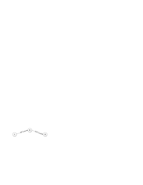
Figure 1: A dual-hop AF relay system in mixed RF and FSO links.

In this letter, based on the model proposed in [9], we firstly study the outage probability and the average symbol error rate (SER) of a dual-hop fixed gain AF system with mixed Rician fading and Gamma-Gamma fading links. We derive the closed-form expressions for the PDF, outage probability (or cumulative distribution function (CDF)) and the average SER in terms of Meijer’s G function.

II System and Channel Models

The system under study is an asymmetric dual-hop AF relay system with no direct link, as shown in Fig.1. The source node S and the destination node D communicate through a relay node R. The first link S-R and the second link R-D are an RF link and an FSO link, respectively. We consider a fixed gain relay. Assume that node S sends a subcarrier signal to node R. At node R, the received signal can be expressed as

$$r_{1}(t)=\alpha_{1}s_{1}(t)+n_{1}(t)$$ (1)

where $\alpha_{1}$ represents the fading gain of the RF link between nodes S and R. $s_{1}(t)$ has an average power $P_{s}$ , and $n_{1}(t)$ is the additive white Gaussian noise (AWGN) with one-side power spectrum density (PSD) of $N_{01}$ . At relay node R, the RF signal $r_{1}(t)$ is used to modulate the irradiance of a continuous wave optical beam at the laser transmitter after being properly biased, then the retransmitted signal can be written as

$$s_{2}(t)=G(1+\xi r_{1}(t))$$ (2)

where $G$ is the fixed relay gain and $\xi$ is the modulation index satisfying the condition $-1\leq\xi r_{1}(t)\leq 1$ in order to avoid overmodulation. For an atmosphere turbulence channel, the received signal at destination node D after direct detection using photodetector can be written as

$$r_{2}(t)=VIAs_{2}(t)+n_{2}(t)$$ (3)

where $V$ is the responsivity of photodetector, $I$ is assumed to be a stationary random variable caused by atmospheric turbulence, $A$ is the area of photodetector, and $n_{2}(t)$ is the AWGN with one-side PSD of $N_{02}$. After removing the direct current (DC) component, the instantaneous end-to-end SNR at the destination node D is given by [2]

$$\gamma=\frac{\gamma_{1}\gamma_{2}}{\gamma_{2}+C}$$ (4)

where $\gamma_{1}=P_{s}\alpha_{1}^{2}/N_{01}$ is the RF link SNR, $\gamma_{2}=(VA\xi)^{2}I^{2}/N_{02}$ is the FSO link SNR, and $C=(G^{2}N_{01})^{-1}$.

Assuming that the RF link is subject to Rician fading, the PDF of $\gamma_{1}$ is given by [12, Eq. 2. 16]

$${f_{{\gamma_{1}}}}\left(r\right)=\left({\frac{{1+{K_{1}}}}{{\overline{{\gamma_{1}}}}}}\right)\exp\left({-{K_{1}}}\right)\exp\left({-\frac{{1+{K_{1}}}}{{\overline{{\gamma_{1}}}}}}\right)$$

$$\times{I_{0}}\left({2\sqrt{{K_{1}}\frac{{1+{K_{1}}}}{{\overline{{\gamma_{1}}}}}r}}\right),r\geq 0$$ (5)

where $\overline{{\gamma_{1}}}={{{P_{s}}}\mathord{\left/{\vphantom{{{P_{s}}}{{N_{01}}}}}\right.\kern-1.2pt}{{N_{01}}}}$ is the RF link’s average SNR, $K_{1}$ is the ratio of the power of the LOS component to the average power of the scattered component and $I_{\alpha}(\cdot)$ is the $\alpha^{th}$-order modified Bessel function of the first kind [13, Eq. 8.406.1]. The CDF of $\gamma_{1}$ is given by

$${F_{{\gamma_{1}}}}(r)=1-{Q_{1}}\left({\sqrt{2{K_{1}}},\sqrt{2\frac{{1+{K_{1}}}}{{\overline{{\gamma_{1}}}}}r}}\right),r\geq 0$$ (6)

where $Q_{i}(\alpha,\beta)$ is the $i^{th}$-order Marcum Q-function [12, Eq. 4. 60]. For the special case of Rayleigh fading, the PDF and CDF of $\gamma_{1}$ can be obtained by substituting $K_{1}=0$ into (5) and (6), respectively. We assume that the FSO link experiences Gamma-Gamma fading, so the PDF of $\gamma_{2}$ is given by [9]

$$f_{\gamma_{2}}(r)=\frac{(\alpha\beta)^{(\alpha+\beta)/2}r^{(\alpha+\beta)/4-1}}{\Gamma(\alpha)\Gamma(\beta)\overline{\gamma_{2}}^{(\alpha+\beta)/4}}$$

$$\times{K_{\alpha-\beta}}\left({2\sqrt{\alpha\beta\sqrt{\frac{r}{{\overline{{\gamma_{2}}}}}}}}\right),r\geq 0$$ (7)

where $\overline{{\gamma_{2}}}={{{{\left({VA\xi}\right)}^{2}}}\mathord{\left/{\vphantom{{{{\left({KA\xi}\right)}^{2}}}{{N_{02}}}}}\right.\kern-1.2pt}{{N_{02}}}}$ is the FSO link s average SNR, $\Gamma(\cdot)$ is the Gamma function [13. Eq. 8. 310. 1] and $K_{\alpha-\beta}(\cdot)$ is the $(\alpha-\beta)^{th}$-order modified Bessel function of the second kind [13, Eq. 8. 432. 9]. The shaping parameters $\alpha$ and $\beta$ are related to the Rytov variance and the relationship $\alpha>\beta$ always holds for FSO communication applications [14].

III Performance Analysis

Firstly, we develop a general framework to obtain the PDF and CDF of the instantaneous end-to-end SNR, $\gamma$, for the fixed gain dual-hop relay systems. The PDF of $\gamma$ is

$${f_{\gamma}}\left(r\right)=\int_{0}^{\infty}{\left({\frac{{{\gamma_{2}}+C}}{{{\gamma_{2}}}}}\right){f_{{\gamma_{1}}}}\left({\frac{{{\gamma_{2}}+C}}{{{\gamma_{2}}}}r}\right){f_{{\gamma_{2}}}}\left({{\gamma_{2}}}\right)d{\gamma_{2}}}$$ (8)

The CDF is the probability that $\gamma$ drops below an SNR threshold $\gamma_{th}$, or mathematically

$$P_{out} =F_{\gamma}(\gamma_{th})=P(\gamma\leq\gamma_{th})$$ (9)

$$=\int_{0}^{\infty}{{F_{{\gamma_{1}}}}\left({\frac{{{\gamma_{2}}+C}}{{{\gamma_{2}}}}{\gamma_{th}}}\right){f_{{\gamma_{2}}}}\left({{\gamma_{2}}}\right)d{\gamma_{2}}}$$

Equations (8) and (9) can be used with any ${f_{{\gamma_{1}}}}\left(r\right)$ and ${f_{{\gamma_{2}}}}\left(r\right)$ to obtain the PDF and CDF of the instantaneous end-to-end SNR for the fixed gain dual-hop relay systems.

III-A The PDF of $\gamma$

The PDF of $\gamma$ is obtained by substituting the expressions (5) and (7) into (8) resulting in

$${f_{\gamma}}\left(r\right) ={A_{0}}{B_{0}}\exp\left({-\frac{{1+{K_{1}}}}{{\overline{{\gamma_{1}}}}}r}\right)$$ (10)

$$\times\int_{0}^{\infty}{\left({1+\frac{C}{x}}\right){x^{\frac{{\alpha+\beta}}{4}-1}}\exp\left({-\frac{{1+{K_{1}}}}{{\overline{{\gamma_{1}}}}}\frac{{Cr}}{x}}\right)}$$

$$\times{I_{0}}\left({2\sqrt{{K_{1}}\frac{{1+{K_{1}}}}{{\overline{{\gamma_{1}}}}}\frac{{x+C}}{x}r}}\right){K_{\alpha-\beta}}\left({2\sqrt{\alpha\beta\sqrt{\frac{x}{{\overline{{\gamma_{2}}}}}}}}\right)dx$$

where

$${A_{0}}=\frac{{1+{K_{1}}}}{{\overline{{\gamma_{1}}}\exp\left({{K_{1}}}\right)}}$$ (11)

$${B_{0}}=\frac{{{{\left({\alpha\beta}\right)}^{\frac{{\alpha+\beta}}{2}}}}}{{\Gamma\left(\alpha\right)\Gamma\left(\beta\right){{\overline{{\gamma_{2}}}}^{\frac{{\alpha+\beta}}{4}}}}}$$ (12)

Using the infinite series representation for the Bessel function ${I_{\alpha}}\left(\cdot\right)$[13, Eq. 8. 447. 1], and the binomial theorem ${\left({1+x}\right)^{n}}=\sum\limits_{k=0}^{n}{\left(\begin{array}[]{l}n\\ k\end{array}\right){x^{k}}}$, we obtain

$$\begin{split}&\left({1+\frac{C}{x}}\right){I_{0}}\left({2\sqrt{{K_{1}}\frac{{1+{K_{1}}}}{{\overline{{\gamma_{1}}}}}\frac{{x+C}}{x}r}}\right)\\ &=\sum\limits_{m=0}^{\infty}{\frac{1}{{{{\left({m!}\right)}^{2}}}}{{\left({{K_{1}}\frac{{1+{K_{1}}}}{{\overline{{\gamma_{1}}}}}r}\right)}^{m}}\sum\limits_{n=0}^{m+1}{\left(\begin{array}[]{l}m+1\\ n\end{array}\right)}}{C^{n}}{x^{-n}}\end{split}$$ (13)

Substituting (13) into (10), we obtain

$$\begin{split}\begin{array}[]{l}{f_{\gamma}}\left(r\right)={A_{0}}{B_{0}}\exp\left({-\frac{{1+{K_{1}}}}{{\overline{{\gamma_{1}}}}}r}\right)\\ \times\sum\limits_{m=0}^{\infty}{\frac{1}{{{{\left({m!}\right)}^{2}}}}{{\left({{K_{1}}\frac{{1+{K_{1}}}}{{\overline{{\gamma_{1}}}}}r}\right)}^{m}}\sum\limits_{n=0}^{m+1}{\left(\begin{array}[]{l}m+1\\ l\end{array}\right)}}{C^{n}}\\ \times\int_{0}^{\infty}{{x^{\frac{{\alpha+\beta}}{4}-n-1}}\exp\left({-\frac{{1+{K_{1}}}}{{\overline{{\gamma_{1}}}}}\frac{{Cr}}{x}}\right)}{K_{\alpha-\beta}}\left({2\sqrt{\alpha\beta\sqrt{\frac{x}{{\overline{{\gamma_{2}}}}}}}}\right)dx\end{array}\end{split}$$ (14)

By expressing the integrands of (14) in terms of Meijer’s G function [15, Eq. 5], according to [15, Eq. 11], [15, Eq. 14], and using [13, Eq. 9. 31. 2] along with [15, Eq. 21], the PDF of $\gamma$ can be obtained as

$$\begin{split}\begin{array}[]{l}{f_{\gamma}}\left(r\right)=\frac{{{A_{0}}{B_{0}}}}{{4\pi}}\exp\left({-\frac{{1+{K_{1}}}}{{\overline{{\gamma_{1}}}}}r}\right)\\ \times\sum\limits_{m=0}^{\infty}{\frac{1}{{{{\left({m!}\right)}^{2}}}}{{\left({{K_{1}}\frac{{1+{K_{1}}}}{{\overline{{\gamma_{1}}}}}r}\right)}^{m}}\sum\limits_{n=0}^{m+1}{\left(\begin{array}[]{l}m+1\\ l\end{array}\right)}}{C^{n}}\\ \times{\left({\frac{{\overline{{\gamma_{1}}}}}{{1+{K_{1}}}}\frac{1}{{Cr}}}\right)^{n-{{\left({\alpha+\beta}\right)}\mathord{\left/{\vphantom{{\left({\alpha+\beta}\right)}4}}\right.\kern-1.2pt}4}}}G_{0,5}^{5,0}\left({\frac{{{{\left({\alpha\beta}\right)}^{2}}\left({1+{K_{1}}}\right)Cr}}{{16\overline{{\gamma_{1}}}\overline{{\gamma_{2}}}}}\left|\begin{array}[]{l}-\\ \Lambda 1\end{array}\right.}\right)\end{array}\end{split}$$ (15)

where

$$\Lambda 1=\left\{{\frac{{\alpha-\beta}}{4},\frac{{\alpha-\beta+2}}{4},\frac{{\beta-\alpha}}{4},\frac{{\beta-\alpha+2}}{4},n-\frac{{\alpha+\beta}}{4}}\right\}$$ (16)

and $G\left(\cdot\right)$ is the Meijer’s G function [15, Eq. 5].

III-B The CDF of $\gamma$

We substitute the expressions (6) and (7) into (9) to obtain the closed-form $F_{\gamma}(\gamma_{th})$. We use the infinite series representation for the Marcum $Q$-function in the CDF of the Rician fading link [12, Eq. 4.64] and the infinite series representation for the Bessel function $I_{\alpha}(\cdot)$ [13, Eq. 8.447.1], and obtain

$$\begin{split}\begin{array}[]{l}{F_{\gamma}}\left({{\gamma_{th}}}\right)=1{\rm{-}}{B_{0}}\exp\left({-{K_{1}}-\frac{{1+{K_{1}}}}{{\overline{{\gamma_{1}}}}}{\gamma_{th}}}\right)\\ \times\sum\limits_{i=0}^{\infty}{\sum\limits_{j=0}^{\infty}{\frac{{K_{1}^{i+j}}}{{j!\left({i+j}\right)!}}{{\left({\frac{{1+{K_{1}}}}{{\overline{{\gamma_{1}}}}}{\gamma_{th}}}\right)}^{j}}}}\sum\limits_{k=0}^{j}{\left(\begin{array}[]{l}j\\ k\end{array}\right){C^{k}}}\\ \times\int_{0}^{\infty}{{x^{\frac{{\alpha+\beta}}{4}-n-1}}\exp\left({-\frac{{1+{K_{1}}}}{{\overline{{\gamma_{1}}}}}\frac{{C{r_{th}}}}{x}}\right)}{K_{\alpha-\beta}}\left({2\sqrt{\alpha\beta\sqrt{\frac{x}{{\overline{{\gamma_{2}}}}}}}}\right)dx\end{array}\end{split}$$ (17)

Similar to deriving (15) from (14), we can obtain the closed-form CDF of $\gamma$ as

$$\begin{split}\begin{array}[]{l}{F_{\gamma}}\left({{\gamma_{th}}}\right)=1-\frac{{{B_{0}}}}{{4\pi}}\exp\left({-{K_{1}}-\frac{{1+{K_{1}}}}{{\overline{{\gamma_{1}}}}}{\gamma_{th}}}\right)\\ \times\sum\limits_{i=0}^{\infty}{\sum\limits_{j=0}^{\infty}{\frac{{K_{1}^{i+j}}}{{j!\left({i+j}\right)!}}{{\left({\frac{{1+{K_{1}}}}{{\overline{{\gamma_{1}}}}}{\gamma_{th}}}\right)}^{j}}}}\sum\limits_{k=0}^{j}{\left(\begin{array}[]{l}j\\ k\end{array}\right){C^{k}}}\\ \times{\left({\frac{{\overline{{\gamma_{1}}}}}{{1+{K_{1}}}}\frac{1}{{C{r_{th}}}}}\right)^{k-{{\left({\alpha+\beta}\right)}\mathord{\left/{\vphantom{{\left({\alpha+\beta}\right)}4}}\right.\kern-1.2pt}4}}}G_{0,5}^{5,0}\left({\frac{{{{\left({\alpha\beta}\right)}^{2}}\left({1+{K_{1}}}\right)C{r_{th}}}}{{16\overline{{\gamma_{1}}}\overline{{\gamma_{2}}}}}\left|\begin{array}[]{l}-\\ \Lambda 2\end{array}\right.}\right)\end{array}\end{split}$$ (18)

where

$$\Lambda 2=\left\{{\frac{{\alpha-\beta}}{4},\frac{{\alpha-\beta+2}}{4},\frac{{\beta-\alpha}}{4},\frac{{\beta-\alpha+2}}{4},k-\frac{{\alpha+\beta}}{4}}\right\}$$ (19)

and $B_{0}$ is defined as (12).

III-C The Average SER

We now derive the expression for the average SER of the system, which is applicable to modulation schemes that have a SER expression of the form as below

$${P_{s}}=aQ\left({\sqrt{2b\gamma}}\right)$$ (20)

where $a$ and $b$ define the modulation schemes (e.g. $a=b=1$ for binary phase shift keying (BPSK), and , $a=2$, $b={\sin^{2}}\left({\pi/M}\right)$ for M-ary phase shift keying (M-PSK)), $Q\left(x\right)=\int_{x}^{\infty}{{{\exp\left({{{-{y^{2}}}\mathord{\left/{\vphantom{{-{y^{2}}}2}}\right.\kern-1.2pt}2}}\right)}\mathord{\left/{\vphantom{{\exp\left({{{-{y^{2}}}\mathord{\left/{\vphantom{{-{y^{2}}}2}}\right.\kern-1.2pt}2}}\right)}{\sqrt{2\pi}}}}\right.\kern-1.2pt}{\sqrt{2\pi}}}}dy$. We give the average SER as

$${P_{s}}=\frac{a}{2}\sqrt{\frac{b}{\pi}}\int_{0}^{\infty}{\frac{{{F_{r}}\left(y\right)}}{{\sqrt{y}}}\exp\left({-by}\right)dy}$$ (21)

Substituting (18) into (21) and using the identities [15, Eq. 11] and [15, Eq. 21], we can get the closed-form average SER as

$$\begin{array}[]{l}{P_{s}}=\frac{a}{2}-\frac{a}{{8\pi}}\sqrt{\frac{b}{\pi}}{B_{0}}\exp\left({-{K_{1}}}\right)\\ \times{\sum\limits_{i=0}^{\infty}{\sum\limits_{j=0}^{\infty}{\frac{{K_{1}^{i+j}}}{{j!\left({i+j}\right)!}}{{\left({\frac{{1+{K_{1}}}}{{\overline{{\gamma_{1}}}}}}\right)}^{j}}\sum\limits_{k=0}^{j}{\left(\begin{array}[]{l}j\\ k\end{array}\right){C^{k}}\left({\frac{{\overline{{\gamma_{1}}}}}{{1+{K_{1}}}}\frac{1}{C}}\right)}}}^{k-{{\left({\alpha+\beta}\right)}\mathord{\left/{\vphantom{{\left({\alpha+\beta}\right)}4}}\right.\kern-1.2pt}4}}}\\ \times{\left({b+\frac{{1+{K_{1}}}}{{\overline{{\gamma_{1}}}}}}\right)^{k-j-{{\left({\alpha+\beta+2}\right)}\mathord{\left/{\vphantom{{\left({\alpha+\beta+2}\right)}4}}\right.\kern-1.2pt}4}}}\\ \times G_{1,5}^{5,1}\left({\frac{{{{\left({\alpha\beta}\right)}^{2}}\left({1+{K_{1}}}\right)C}}{{16\overline{{\gamma_{2}}}\left({1+{K_{1}}+b\overline{{\gamma_{1}}}}\right)}}\left|\begin{array}[]{l}\frac{1}{2}-j+k-\frac{{\alpha+\beta}}{4}\\ \Lambda 2\end{array}\right.}\right)\end{array}$$ (22)

where ${B_{0}}$ is defined as (12) and $\Lambda 2$ is defined as (19).

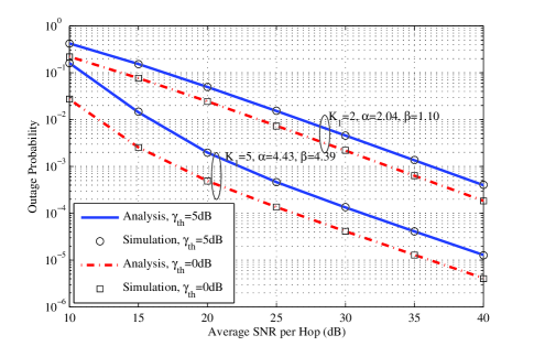
Figure 2: Outage probability with threshold $\gamma_{th}=0,5$dB.

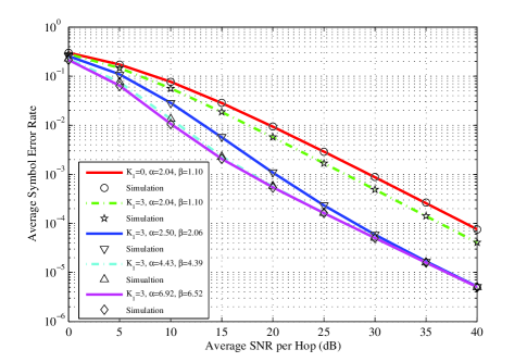
Figure 3: Average SER with fixed Rician parameter $K_{1}=3$. The lines represent the analytical results.

IV Numerical and Simulation Results

In this section, we compare the theoretical results in Section III with the simulations results. We assume equal noise PSD, $N_{0}$, at the relay and the destination, and the balanced links, $\overline{{\gamma_{1}}}=\overline{{\gamma_{2}}}=\overline{\gamma}$. $C$ is set to 1. Each of the infinite summations in (18) and (22) was truncated at the $35th$ term, because adding more terms does not affect the results in the $15th$ decimal place.

Fig. 2 presents the outage probability versue average SNR per hop of the dual-hop AF systems operating over two groups of mixed fading channels. The outage threshold $\gamma_{th}$ is set to 0 and 5dB, respectively. It is observed that the numerical results of (18) match well with the simulation results. Further, as expected, the outage probability decreases with increasing average SNR per hop and increases with severer fading channels and higher threshold values.

Fig. 3 shows the effects of the Gamma-Gamma fading parameters, $\alpha$ and $\beta$, on the average SER of the dual-hop AF systems employing BPSK modulation. Fig. 3 presents the average SER of the dual-hop AF systems with $K_{1}=3$ and different $\left({\alpha,\beta}\right)$ pairs. $\left({\alpha=6.92,\beta=6.52}\right)$, $\left({\alpha=4.43,\beta=4.39}\right)$, $\left({\alpha=2.50,\beta=2.06}\right)$, and $\left({\alpha=2.04,\beta=1.10}\right)$ represent the weaker, weak, moderate, and strong Gamma-Gamma turbulence conditions, respectively. The average SER of a dual-hop AF system operating over Rayleigh fading link $\left({{K_{1}}=0}\right)$ is shown for comparison. It is shown that the numerical results of (22) agree well with the simulation results. As expected, it is observed that the average SER is improved when the Gamma-Gamma turbulence condition becomes weaker. However, it is observed that the limiting slopes of the average SER curves for the different cases of turbulence conditions are the same as the limiting slope of the curve for the case of Rayleigh fading link and Gamma-Gamma parameters $\left({\alpha=2.04,\beta=1.10}\right)$. Moreover, Fig. 3 presents that the average SER improvement can become negligible when the turbulence conditions become weaker.

Fig. 4 shows the effects of Rician fading parameter $K_{1}$ on the average SER of the dual-hop AF systems employing BPSK modulation. The dual-hop AF system with fixed Gamma-Gamma parameters $\left({\alpha=2.50,\beta=2.06}\right)$ and different Rician fading parameters, $K_{1}$ = 2, 4, 6, and 8, are investigated. The average SER of a dual-hop AF system operating over Rayleigh fading link $\left({{K_{1}}=0}\right)$ is shown for comparison. Fig. 4 shows that the numerical results of (22) match with the simulation results. It can be seen from Fig. 4 that the average SER is improved, as expected, with an increase of parameter $K_{1}$. As observed in Fig. 3, the limiting slopes of the average SER curves for the different cases of $K_{1}$ are the same as the limiting slope of the curve for the case of Rayleigh fading link. However, in contrast to the results shown in Fig. 3, there is a remarkable SNR gain when the Rician fading parameter $K_{1}$ becomes larger. Based on Fig. 3 and Fig. 4, we conclude that the Rician fading parameter has a great impact on the average SER of the dual-hop fixed gain AF systems operating over the mixed Rician and Gamma-Gamma turbulence links.

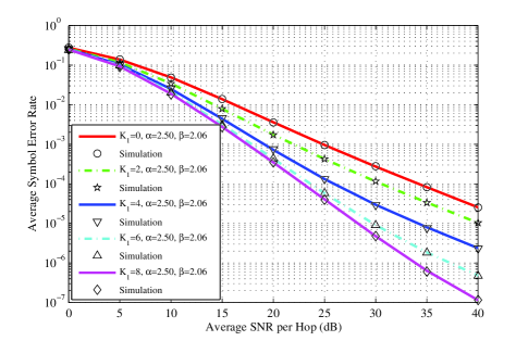
Figure 4: Average SER with fixed Gamma-Gamma parameters, $\alpha=2.50$, $\beta=2.06$. The lines represent the analytical results.

V Conclusion

In this letter, we have derived the closed-form expressions for the PDF, the CDF, and the average SER of a dual-hop fixed gain AF relaying systems operating over the mixed Rician fading and Gamma-Gamma turbulence links. The simulation results are given to validate the analytical ones. The results show that the limiting slopes of the CDF and the average SER only depend on the Rayleigh fading, irrespective of the Gamma-Gamma turbulence conditions.

References

- [1] J. N. Laneman, D. N. Tse, and G. W. Wornell, “Cooperative diversity in wireless network: efficient protocols and outage behaviour,” IEEE Trans. Inf. Theory, vol. 50, no. 12, pp. 3062-3080, Dec. 2004.
- [2] M. O. Hasna and M.-S. Alouini, “A performance study of dual-hop transmission with fixed gain relays,” IEEE Trans. Wireless Commun., vol. 3, no. 6, pp. 1963-1968, Nov. 2004.
- [3] Y. Zhu, Y. Xin, and P.-Y. Kam, “Outage probability of Rician fading relay channels,” IEEE Trans. Veh. Technol., vol. 57, no. 4, pp. 2648-2652, Jul. 2008.
- [4] M. Xia, Y.-C. Wu, and S. Aissa, “Exact outage probability of dual-hop CSI-assisted AF relaying over Nakagami-m fading channels,” IEEE Trans. Signal Process., vol. 60, no. 10, pp. 5578-5583, Oct. 2012.
- [5] H. A. Suraweera, R. H. Y. Louie, Y. Li, G. K. Karagiannidis, and B. Vucetic, “Two hop amplify-and-forward relay in mixed Rayleigh and Rician fading channels,” IEEE Commun. Lett., vol. 13, no. 4, pp. 227-229, Apr. 2009.
- [6] S. S. Soliman and N. C. Beaulieu, “Dual-hop AF relaying systems in mixed Nakagami-m and Rician links,” in Proc. Globecom Workshops (GC Wkshps), Anaheim, CA, pp. 447-452, Dec. 2012.
- [7] X. Zhu and J. M. Kahn, “Free-space optical communication through atmospheric turbulence channels,” IEEE Trans. Commun., vol. 50, pp. 1293-1300, Aug. 2002.
- [8] M. Safari and M. Uysal, “Cooperative diversity over log-normal fading channels: performance analysis and optimization,” IEEE Trans. Wireless Commun., vol. 7, no. 5, pp. 1963-1972, May 2008.
- [9] E. Lee, J. Park, D. Han, and G. Yoon, “Performance analysis of the asymmetric dual-hop relay transmission with mixed RF/FSO links,” IEEE Photon. Technol. Lett., vol. 23, no. 21, pp. 1642-1644, Nov. 2011.
- [10] I. S. Ansari, F. Yilmaz, and M.-S. Alouini, “On the performance of mixed RF/FSO dual-hop transmission systems,” in Proc. IEEE 77th Vehicular Technology Conference (VTC Spring 2013), Dresden, Germany, Jun. 2013.
- [11] I. S. Ansari, F. Yilmaz, and M.-S. Alouini, “Impact of pointing errors on the performance of mixed RF/FSO dual-hop transmission systems,” IEEE Wireless Commun. Lett., vol. 2, no. 3, pp. 351-354, Jun. 2013.
- [12] M. K. Simon and M.-S. Alouini, Digital Communication over Fading Channels, 2nd ed. New York: Wiley, 2005.
- [13] I. S. Gradshteyn and I. M. Ryzhik, Table of Integrals, Series, and Products, 7th ed. San Diego: Academic, 2007.
- [14] N. Wang and J. Cheng, “Moment-based estimation for the shape parameters of the Gamma-Gamma atmospheric turbulence model,” Opt. Express, vol. 18, pp. 12824-12831, June 2010.
- [15] V. S. Adamchik and O. I. Marichev, “The algorithm for calculating integral of hypergeomtric type functions and its realization in reduce system,” in Proc. Int. Conf. Symbolic and Algebraic Computation, Tokyo, Japan, pp. 212-224, 1990.