Neural Text Generation: A Practical Guide

Abstract

Deep learning methods have recently achieved great empirical success on machine translation, dialogue response generation, summarization, and other text generation tasks. At a high level, the technique has been to train end-to-end neural network models consisting of an encoder model to produce a hidden representation of the source text, followed by a decoder model to generate the target. While such models have significantly fewer pieces than earlier systems, significant tuning is still required to achieve good performance. For text generation models in particular, the decoder can behave in undesired ways, such as by generating truncated or repetitive outputs, outputting bland and generic responses, or in some cases producing ungrammatical gibberish. This paper is intended as a practical guide for resolving such undesired behavior in text generation models, with the aim of helping enable real-world applications.

[Language makes] infinite use of finite means.

On Language
Wilhelm von Humboldt

But Noodynaady’s actual ingrate tootle is of come into the garner mauve and thy nice are stores of morning and buy me a bunch of iodines.

Finnegans Wake
James Joyce

1 Introduction

Neural networks have recently attained state-of-the-art results on many tasks in machine learning, including natural language processing tasks such as sentiment understanding and machine translation. Within NLP, a number of core tasks involve generating text, conditioned on some input information. Prior to the last few years, the predominant techniques for text generation were either based on template or rule-based systems, or well-understood probabilistic models such as $n$-gram or log-linear models (Chen and Goodman, 1996; Koehn et al., 2003). These rule-based and statistical models, however, despite being fairly interpretable and well-behaved, require infeasible amounts of hand-engineering to scale—in the case of rule or template-based models—or tend to saturate in their performance with increasing training data (Jozefowicz et al., 2016). On the other hand, neural network models for text, despite their sweeping empirical success, are poorly understood and sometimes poorly behaved as well. Figure 1 illustrates the trade-offs between these two types of systems.

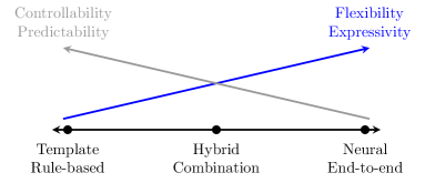
Figure 1: Figure illustrating the tradeoffs between using rule-based vs. neural text generation systems.

To help with the adoption of more usage of neural text generation systems, we detail some practical suggestions for developing NTG systems. We include a brief overview of both the training and decoding procedures, as well as some suggestions for training NTG models. The primary focus, however, is advice for diagnosing and resolving pathological behavior during decoding. As it can take a long time to retrain models, it is comparatively cheap to tune the decoding procedure; hence it’s worth understanding how to do this quickly before deciding whether or not to retrain.

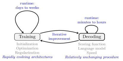
Figure 2: Development cycle for NTG systems.

Figure 2 illustrates the feedback loops when improving different components of the model training and decoding procedures.

Despite a growing body of research, information on best practices tends to be scattered and often depends on specific model architectures. While some starting hyperparameters are suggested, the advice in this guide is intended to be as architecture-agnostic as possible, and error analysis is emphasized instead. It may be helpful to first read the background section, but the remaining sections can be read independently.

1.1 Focus of this guide

This guide focuses on advice for training and decoding of neural encoder-decoder models (with an attention mechanism) for text generation tasks. Roughly speaking, the source and target are assumed to be on the order of dozens of tokens. The primary focus of the guide is on the decoding procedure. Besides suggestions for improving the model training and decoding algorithms, we also touch briefly on preprocessing (Section 3) and deployment (Section 5.3).

1.1.1 Limitations: What will not be covered

Before continuing, we describe what this guide will not cover, as well as some of the current limitations of neural text generation models. This guide does not consider:

• Natural language understanding and semantics. While impressive work has been done in learning word embeddings (Mikolov et al., 2013; Pennington et al., 2014), the goal of learning “thought vectors” for sentences has remained more elusive (Kiros et al., 2015). As previously mentioned, we also do not consider sequence labeling or classification tasks.

• How to capture long-term dependencies (beyond a brief discussion of attention) or maintain global coherence. This remains a challenge due to the curse of dimensionality as well as neural networks failing to learn more abstract concepts from the predominant next-step prediction training objective.

• How to interface models with a knowledge base, or other structured data that cannot be supplied in a short piece of text. Some recent work has used pointer mechanisms towards this end (Vinyals et al., 2015).

• Consequently, while we focus on natural language, to be precise, this guide does not cover natural language generation (NLG), which entails generating documents or longer descriptions from structured data. The primary focus is on tasks where the target is a single sentence—hence the term “text generation” as opposed to “language generation”.

Although the field is evolving quickly, there are still many tasks where older rule or template-based systems are the only reasonable option. Consider, for example, the seminal work on ELIZA (Weizenbaum, 1966)—a computer program intended to emulate a psychotherapist—that was based on pattern matching and rules for generating responses. In general, neural-based systems are unable perform the dialogue state management required for such systems. Or consider the task of generating a summary of a large collection of documents. With the soft attention mechanisms used in neural systems, there is currently no direct way to condition on such an amount of text.

2 Background

Summary of Notation

Symbol	Shape	Description
$V$	scalar	size of output vocabulary
$X$	$S$	input/source sequence $(x_{1},\dots,x_{S})$ of length $S$
$Y$	$T$	output/target sequence $(y_{1},\dots,y_{T})$ of length $T$
$E$	$(S,h)$	encoder hidden states where $E_{j}$ denotes representation at timestep $j$
$D$	$(T,h)$	decoder hidden states where $D_{i}$ denotes representation at timestep $i$
$A$	$(T,S)$	attention matrix where $A_{ij}$ is attention weight at $i$th decoder timestep on $j$th encoder state representation
$H$	varies	hypothesis in hypothesis set $\mathcal{H}$ during decoding
$s(H)$	scalar	score of hypothesis $H$ during beam search

Minibatch size dimension is omitted from the shape column.

2.1 Setting

We consider modeling discrete sequences of text tokens. Given a sequence $U=(u_{1},u_{2},\dots,u_{S})$ over the vocabulary $V$, we seek to model

$$p(U)=\prod_{t=1}^{S}p(u_{t}|u_{<t})$$ (1)

where $u_{<t}$ denotes $u_{1},u_{2},\dots,u_{t-1}$, and equality follows from the chain rule of probability. Depending on how we choose to tokenize the text, the vocabulary can contain the set of characters, word-pieces/byte-pairs, words, or some other unit. For the tasks we consider in this paper, we divide the sequence $U$ into an input or source sequence $X$ (that is always provided in full) and an output or target sequence $Y$. For example, for machine translation tasks $X$ might be a sentence in English and $Y$ the translated sentence in Chinese. In this case, we model

$$p(Y|X)=\prod_{t=1}^{T}p(y_{t}|X,y_{<t})$$ (2)

Task	$X$ (example)	$Y$ (example)
language modeling	none (empty sequence)	tokens from news corpus
machine translation	source sequence in English	target sequence in French
grammar correction	noisy, ungrammatical sentence	corrected sentence
summarization	body of news article	headline of article
dialogue	conversation history	next response in turn
Related tasks (may be outside scope of this guide)
speech transcription	audio / speech features	text transcript
image captioning	image	caption describing image
question answering	supporting text + knowledge base + question	answer

Table 1: Example tasks we consider.

Note that this is a generalization of (1); we consider $p(Y|X)$ from here on. Besides machine translation, this also encompasses many other tasks in natural language processing—see Table 1 for a summary.

Beyond the tasks described in the first half of Table 1, many of the techniques described in this paper also extend to tasks at the intersection of text and other modalities. For example, in speech recognition, $X$ may be a sequence of features computed on short snippets of audio, with $Y$ being the corresponding text transcript, and in image captioning $X$ is an image (which is not so straightforward to express as a sequence) and $Y$ the corresponding text description. While we could also include sequence labeling (for example part-of-speech tagging) as another task, we instead consider tasks that do not have a clear one-to-one correspondence or between source and target. The lack of such a correspondence leads to issues in decoding which we focus on in Section 5. The same reasoning applies to sequence classification tasks such as sentiment analysis.

2.2 Encoder-decoder models

Encoder-decoder models, also referred to as sequence-to-sequence models, were developed for machine translation and have rapidly exceeded the performance of prior systems depite having comparatively simple architectures, trained end-to-end to map source directly to target.

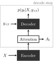
Figure 3: Figure illustrating the generic encoder-decoder model architecture we assume for this guide. Several choices are possible for the encoder and decoder architectures as well as for the attention mechanism. Here we show the outputs for a single timestep.

Before neural network-based approaches, count-based methods (Chen and Goodman, 1996) and methods involving learning phrase pair probabilities were used for language modeling and translation. Prior to more recent encoder-decoder models, feed-forward fully-connected neural networks were shown to work well for language modeling. Such models simply stack affine matrix transforms followed by nonlinearities to the input and each following hidden layer (Bengio et al., 2003). However, these networks have fallen out of favor for modeling sequence data, as they require defining a fixed context length when modeling $p(y_{t}|X,y_{<t})$, do not use parameter sharing across timesteps, and have been surpassed in performance by subsequent architectures.

At the time of this writing, several different architectures have demonstrated strong results.

• Recurrent neural networks (RNNs) use shared parameter matrices across different time steps and combine the input at the current time step with the previous hidden state summarizing all previous time steps (Mikolov et al., 2010; Sutskever et al., 2014; Cho et al., 2014). Many different gating mechanisms have been developed for such architectures to try and ease optimization (Hochreiter and Schmidhuber, 1997; Cho et al., 2014).

• Convolutional neural networks (CNNs). Convolutions with kernels reused across timesteps can also be used with masking to avoid peeking ahead at future inputs during training (see Section 2.3 for an overview of the training procedure) (Kalchbrenner et al., 2016). Using convolutions has the benefit during training of parallelizing across the time dimension instead of computing the next hidden state one step at a time.

• Both recurrent and convolutional networks for modeling sequences typically rely on a per timestep attention mechanism (Bahdanau et al., 2014) that acts as a shortcut connection between the target output prediction and the relevant source input hidden states. At a high-level, at decoder timestep $i$, the decoder representation $D_{i}$ is used to compute a weight $\alpha_{ij}$ for each encoder representation $E_{j}$. For example, this could be done by using the dot product $D_{i}^{\top}E_{j}$ as the logits before applying the softmax function. Hence

  $$\alpha_{ij}=\exp(D_{i}^{\top}E_{j})/\sum_{k=1}^{S}\exp(D_{i}^{\top}E_{k})$$

  The weighted representation $\sum_{j=1}^{S}\alpha_{ij}E_{j}$ is then fed into the decoder along with $X$ and $y_{<i}$. More recent models which rely purely on attention mechanisms with masking have also been shown to obtain as good or better results as RNN or CNN-based models (Vaswani et al., 2017). We describe the attention mechanism in more detail in Section 2.5.

Unless otherwise indicated, the advice in this guide is intended to be agnostic of the model architecture, as long as the following two conditions hold:

1. The model performs next-step prediction of the next target conditioned on the source and previous predicted targets, i.e. it models $p(y_{t}|X,y_{<t})$.

2. The model uses an attention mechanism (resulting in an attention matrix $A$), which eases training, is simple to implement and cheap to compute in most cases, and has become a standard component of encoder-decoder models.

Figure 3 illustrates the backbone architecture we use for this guide.

2.3 Training overview

During training, we optimize over the model parameters $\theta$ the sequence cross-entropy loss

$$\ell(\theta)=-\sum_{t=1}^{T}\log p(y_{t}|X,y_{<t};\theta).$$ (3)

thus maximizing the log-likelihood of the training data. Previous ground truth inputs are given to the model when predicting the next index in the sequence, a training method sometimes referred to (unfortunately) as teacher forcing. Due to the inability to fit current datasets into memory as well as for faster convergence, gradient updates are computed on minibatches of training sentences. Stochastic gradient descent (SGD) as well as optimizers such as Adam (Kingma and Ba, 2014) have been shown to work well empirically.

Recent reserarch has also explored other methods for training sequence models, such as by using reinforcement learning or a separate adversarial loss (Goodfellow et al., 2014; Li et al., 2016b, 2017; Bahdanau et al., 2016; Arjovsky et al., 2017). As of this writing, however, the aforementioned training method is the primary workhorse for training such models.

2.4 Decoding overview

During decoding, we are given the source sequence $X$ and seek to generate the target $\hat{Y}$ that maximizes some scoring function $s(\hat{Y})$. In greedy decoding, we simply take the argmax over the softmax output distribution for each timestep, then feed that as the input for the next timestep. Thus at any timestep we only have a single hypothesis. Although greedy decoding can work surprisingly well, note that it often does not result in the most probable output hypothesis, since there may be a path that is more probable overall despite including an output which was not the argmax (this also holds true for most scoring functions we may choose).

Since it’s usually intractable to consider every possible $\hat{Y}$ due to the branching factor and number of timesteps, we instead perform beam search, where we iteratively expand each hypotheses one token at a time, and at the end of every search iteration we only keep the $k$ best (in terms of $s(\cdot)$) hypotheses, where $k$ is the beam width or beam size. Here’s the full beam search procedure, in more detail:

1. We begin the beam procedure with the start-of-sequence token, $\langle\mathrm{sos}\rangle$. Thus our set of hypothesis $\mathcal{H}=\{[\langle\mathrm{sos}\rangle]\}$ consisting of the single hypothesis $H=[\langle\mathrm{sos}\rangle]$, a list with only the start token.

2. Repeat, for $t=1,2,\dots,T_{\mathrm{max}}$:

   1. Repeat, for $H\in\mathcal{H}$:

      1. Repeat, for every $u$ in the vocabulary $V$ with probability $p_{ut}=p(u|X,H)$:

         1. Add the hypothesis $H_{\mathrm{new}}=[\langle\mathrm{sos}\rangle,h_{1},\dots,h_{t-1},u]$ to $\mathcal{H}$.

         2. Compute and cache $s(H_{\mathrm{new}})$. For example, if $s(\cdot)$ simply computes the cumulative log-probability of a hypothesis, we have $s(H_{\mathrm{new}})=s(H)+\log p_{ut}$.

   2. If any of the hypotheses end with the end-of-sequence token $\langle\mathrm{eos}\rangle$ , move that hypothesis to the list of terminated hypotheses $\mathcal{H}_{\mathrm{final}}$.

   3. Keep the $k$ best remaining hypotheses in $\mathcal{H}$ according to $s(\cdot)$.

3. Finally, we return $H^{*}=\mathrm{arg}\max_{H\in\mathcal{H}_{\mathrm{final}}}s(H)$. Since we are now considering completed hypotheses, we may also wish to use a modified scoring function $s_{\mathrm{final}}(\cdot)$.

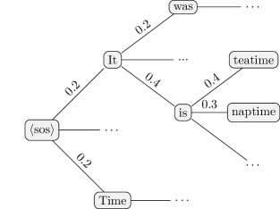
Figure 4: Toy example of beam search procedure with beam width $k=2$. The search has been run for 3 steps and no hypothesis has terminated with $\langle\mathrm{eos}\rangle$ yet. Edges are annotated with probabilities of tokens. Only the tokens after pruning to the top $k$ hypotheses are shown.

One surprising result with neural models is that relatively small beam sizes yield good results with rapidly diminishing returns. Further, larger beam sizes can even yield (slightly) worse results. For example, a beam size of 8 may only work marginally better than a beam size of 4, and a beam size of 16 may work worse than 8 (Koehn and Knowles, 2017).

Finally, oftentimes incorporating a language model (LM) in the scoring function can help improve performance. Since LMs only need to be trained on the target corpus, we can train language models on much larger corpuses that do not have parallel data. Our objective in decoding is to maximize the joint probability:

$$\mathrm{arg}\max_{\hat{Y}}p(X,\hat{Y}) =\mathrm{arg}\max_{\hat{Y}}p(X|\hat{Y})p(\hat{Y})$$ (4)

However, since we are given $X$ and not $Y$, it’s intractable to maximize over $p(X|\hat{Y})$. In practice, we instead maximize the pseudo-objective

$$\mathrm{arg}\max_{\hat{Y}}p(\hat{Y}|X)p(\hat{Y}).$$

If our original score is $s(H)$, which we assume involves a $p(H|X)$ term, then the LM-augmented score is

$$s(H)+\lambda\log p_{\mathrm{LM}}(H)$$

where $\lambda$ is a hyperparameter to balance the LM and decoder scores.

Despite these issues, this simple procedure works fairly well. However, there arise many cases where beam search, with or without a language model, can result in far from optimal outputs. This is due to inherent biases in the decoding (as well as the training) procedure. We describe how to diagnose and tackle these problems that can arise in Section 5.

2.5 Attention

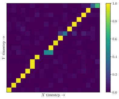
Figure 5: Expected attention matrix $A$ when source and target are monotonically aligned (synthesized as illustrative example).

The basic attention mechanism used to “attend” to portions of the encoder hidden states during each decoder timestep has many extensions and applications. Attention can also be over previous decoder hidden states, in what is called self-attention (Vaswani et al., 2017), or used over components separate from the encoder-decoder model instead of over the encoder hidden states Grave et al. (2016). It can also be used to monitor training progress (by inspecting whether a clear alignment develops between encoder and decoder hidden states), as well as to inspect the correspondences between the input and output sequence that the network learns.

That last bit—that the attention matrix $A$ typically follows the correspondences between input and output—will be useful when we discuss methods for guiding the decoding procedure in Section 5. Hence we go into more detail on the attention matrix $A$ here.

The attention matrix $A$ has $T$ columns and $S$ rows, where $T$ is the number of output timesteps and $S$ is the number of input timesteps. Every row $A_{i}$ is a discrete probability distribution over the encoder hidden states, which in this guide we assume to be equal to the number of input timesteps $S$. In the case that a encoder column $A_{:j}$ has no entry over some threshold (say $0.5$), this suggests that the corresponding encoder input was ignored by the decoder. Likewise, if $A_{:j}$ has multiple values over threshold, this suggests those encoder hidden states were repeatedly used during multiple decoder timesteps. Figure 5 shows an attention matrix we might expect for a well-trained network where source and target are well-aligned (e.g. English$\rightarrow$French translation). For a great overview and visualizations of of attention and RNN models, also see Olah and Carter (2016).

2.6 Evaluation

One of the key challenges for developing text generation systems is that there is no satisfying automated metric for evaluating the final output of the system. Unlike classification and sequence labeling tasks, we (as of now) cannot precisely measure the output quality of text generation systems barring human evaluation. Perplexity does not always correlate well with downstream metrics (Chen et al., 1998), automated or otherwise. Common metrics based on $n$-gram overlap such as ROUGE (Lin, 2004) and BLEU (Papineni et al., 2002) are only rough approximations, and often do not capture linguistic fluency and cohererence (Conroy and Dang, 2008; Liu et al., 2016). Such metrics are especially problematic in more open-ended generation tasks such as summarization and dialogue.

Recent results have shown that though automated metrics are not great at distinguishing between systems once performance passes some baseline, they nonetheless are useful for finding examples where performance is poor, and can also be consistent for evaluating similar systems (Novikova et al., 2017). Thus, despite issues with current automated evaluation metrics, we assume their use for model development; however, manual human evaluation should be interspersed as well.

3 Preprocessing

With increasingly advanced libraries for building computation graphs and performing automatic differentiation, a more significant portion of the software development process is devoted to data preparation.

Broadly speaking, once the raw data has been collected, there remains cleaning, tokenization, and splitting into training and test data. An important consideration during cleaning is setting the character encoding—for example ASCII or UTF-8—for which libraries such as Python’s unidecode can save a lot of time. After cleaning comes the less easily-specified tasks of splitting the text into sentences and tokenization. At present, we recommend Stanford CoreNLP for extensive options and better handling of sentence and word boundaries than other available libraries.

An alternative to performing tokenization (and later detokenization) is to avoid it altogether. Instead of working at the word level, we can instead operate at the character level or use intermediate subword units (Sennrich et al., 2015). Such models result in longer sequences overall, but empirically subword models tend to provide a good trade-off between sequence length (speed) and handling of rare words (Wu et al., 2016). Section 5.2.1 discusses the benefits of subword models in more detail. Ultimately, if using word tokens, it’s important to use a consistent tokenization scheme for all inputs to the system—this includes handling of contractions, punctuation marks such as quotes and hyphens, periods denoting abbreviations (nonbreaking prefixes) vs. sentence boundaries, character escaping, etc.

4 Training

A few heuristics should be sufficient for handling many of the issues when training such models. Start by getting the model to overfit on a tiny subset of the data as a quick sanity check. If the loss explodes, keep reducing the learning rate until it doesn’t. If the model overfits, apply dropout (Srivastava et al., 2014; Zaremba et al., 2014) and weight decay until it doesn’t. Gradient clipping is often crucial to avoid the exploding gradient problem while using a reasonably large learning rate. For SGD and its variants, periodically annealing the learning rate when the validation loss fails to decrease typically helps significantly.

A few useful heuristics that should be robust to the hyperparameter settings and optimization settings you use:

• Sort the next dozen or so batches of sentences by length so each batch has examples of roughly the same length, thus saving computation (Sutskever et al., 2014).

• If the training set is small, tuning regularization will be key to performance (Melis et al., 2017). Noising (or “token dropout”) is also worth trying (Xie et al., 2017). Though we only touch on this issue briefly, amount of training data will be in most cases the primary bottleneck in the performance of a NTG model.

• Measure validation loss after each epoch and anneal the learning rate when validation loss stops decreasing. Depending on how much the validation loss fluctates (based off of validation set size and optimizer settings) you may wish to anneal with patience (wait for several epochs of non-decreasing learning rate before reducing the learning rate).

• Periodically checkpoint model parameters and measure downstream performance (BLEU, $F_{1}$, etc.) using several of the last few model checkpoints. Validation cross entropy loss and final performance may not correlate well, and there can be significant differences in final performance across checkpoints with similar validation losses.

• Ensembling almost always improves performance. Averaging checkpoints is a cheap way to approximate the ensembling effect (Huang et al., 2017).

For a survey of model parameters to consider as well as suggested settings of hyperparameters, see Britz et al. (2017) or Melis et al. (2017).

5 Decoding

Suppose you’ve trained a neural network encoder-decoder model that achieves reasonable perplexity on the validation set. You then try running decoding or generation using this model. The simplest way is to run greedy decoding, as described in Section 2.4. From there, beam search decoding should yield some additional performance improvements. However, it’s rare that things simply work. This section is intended for use as a quick reference when encountering common issues during decoding.

5.1 Diagnostics

First, besides manual inspection, it’s helpful to create some diagnostic metrics when debugging the different components of a text generation system. Despite training the encoder-decoder network to map source to target, during the decoding procedure we introduce two additional components:

1. A scoring function $s(H)$ that tells us how “good” a hypothesis $H$ on the beam is.

2. Optionally, a language model trained on a large corpus which may or may not be similar to the target corpus.

It may not be clear which of these components we should prioritize when trying to improve the performance of the combined system; hence it can be very helpful to run ablative analysis (Ng, 2007),

For the language model, a few suggestions are measuring performance for $\lambda=0$ and several other reasonably spaced values, then plotting the performance trend; measuring perplexity of the language model when trained on varying amounts of training data, to see if more data would be helpful or yields diminishing returns; and measuring performance when training the language model on several different domains (news data, Wikipedia, etc.) in cases where it’s difficult to obtain data close to the target domain.

When measuring the scoring function, computing metrics and inspecting the decoded outputs vs. the gold sentences often immediately yields insights. Useful metrics include:

• Average length of decoded outputs $\hat{Y}$ vs. average length of reference targets $Y$.

• $s(\hat{Y})$ vs. $s(Y)$, then inspecting the ratio $s(\hat{Y})/s(Y)$. If the average ratio is especially low, then there may be a bug in the beam search, or the beam size may need to be increased. If the average ratio is high, then the scoring function may not be appropriate.

• For some applications computing edit distance (insertions, substitutions, deletions) between $\hat{Y}$ and $Y$ may also be useful, for example by looking at the most frequent edits or by examining cases where the length-normalized distances are highest.

5.2 Common issues

5.2.1 Rare and out-of-vocabulary (OOV) words

Decoded	And as in $\langle\mathrm{unk}\rangle$ thought he stood, The $\langle\mathrm{unk}\rangle$, with eyes of flame$\langle\mathrm{eos}\rangle$
Expected	And as in uffish thought he stood, The Jabberwock, with eyes of flame$\langle\mathrm{eos}\rangle$

For languages with very large vocabularies, especially languages with rich morphologies, rare words become problematic when choosing a tokenization scheme that results in more token labels than it is feasible to model in the output softmax. One ad hoc approach that was first used to deal with this issue is simply to truncate the softmax output size (to say, 50K), then assign the remaining token labels all to the $\langle\mathrm{unk}\rangle$ class (Luong et al., 2014). The box above illustrates the resulting output (after detokenization) when rare words are replaced with $\langle\mathrm{unk}\rangle$s. A more elegant approach is to use character or subword preprocessing (Sennrich et al., 2015; Wu et al., 2016) to avoid OOVs entirely, though this can slow down runtime for both training and decoding.

5.2.2 Decoded output short, truncated or ignore portions of input

Decoded	It’s no use going back to yesterday.$\langle\mathrm{eos}\rangle$
Expected	It’s no use going back to yesterday, because I was a different person then.$\langle\mathrm{eos}\rangle$

During the decoding search procedure, hypotheses terminate with the $\langle\mathrm{eos}\rangle$ token. The decoder network should learn to place very low probability on the $\langle\mathrm{eos}\rangle$ token until the target is fully generated; however, sometimes $\langle\mathrm{eos}\rangle$ does not have sufficiently low probability. This is because as the length of the hypothesis grows, the total log probability only decreases. Thus, if we do not normalize the log probability by the length of the hypothesis, shorter hypotheses will be favored. The box above illustrates an example where the hypothesis terminates early. This issue is exacerbated when incorporating a language model term. Two simple ways of resolving this issue are normalizing the log-probability score and adding a length bonus.

• Length normalization: Replace the score $s(\hat{Y})$ with the score normalized by the hypothesis length $s(\hat{Y})/\hat{T}$.

• Length bonus: Replace the score $s(\hat{Y})$ with the $s(\hat{Y})+\beta\hat{T}$, where $\beta>0$ is a hyperparameter.

Note that normalizing the total log-probability by length is equivalent to maximizing the $\hat{T}$^th root of the probability, while adding a length bonus is equivalent to multiplying the probability at every timestep by a baseline $e^{\beta}$.

Figure 6: Example of attention matrix $A$ when decoding terminates early with the $\langle\mathrm{eos}\rangle$ token without having covered the input $X$.

Another method for avoiding this issue is with a coverage penalty using the attention matrix $A$ (Tu et al., 2016; Wu et al., 2016). As formulated here, the coverage penalty can only be applied once a hypothesis (with a corresponding attention matrix) has terminated; hence it can only be incorporated into $s_{\mathrm{final}}(\cdot)$ to perform a final re-ranking of the hypotheses. For a given hypothesis $H$ with attention matrix $A$ with shape $(\hat{T},S)$, the coverage penalty is computed as

$$\mathrm{cp}(A)=\sum_{j=1}^{S}\log\left[\min\left(\sum_{i=1}^{\hat{T}}A_{ij},1.0\right)\right]$$ (5)

Intuitively, for every source timestep, if the attention matrix places full probability on that source timestep when aggregated over all decoding timesteps, then the coverage penalty is zero. Otherwise a penalty is incurred for not attending to that source timestep.

Finally, when the source and target are expected to be of roughly equal lengths, one last trick is to simply constrain the target length $\hat{T}$ to be within some delta of the source length $S$, e.g. $\max(S-\delta,(1-\Delta)\cdot S)\leq\hat{T}\leq\max(S+\delta,(1+\Delta)\cdot S)$ where we also include $S-\delta$ and $S+\delta$ in the case where $S$ is very small, and $\delta$ and $\Delta$ are hyperparameters.

5.2.3 Decoded output repeats

Decoded	I’m not myself, you see, you see, you see, you see, …
Expected	I’m not myself, you see.$\langle\mathrm{eos}\rangle$

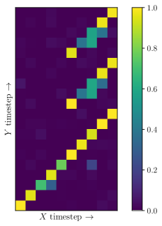
Figure 7: Example of attention matrix $A$ when decoding exhibits repeating behavior.

Repeating outputs are a common issue that often seem to expose neural versus template-based systems. Simple measures include adding a penalty when the model reattends to previous timesteps after the attention has shifted away. This is easily detected using the attention matrix $A$ with some manually selected threshold.

Finally, a more fundamental issue to consider with repeating outputs is poor training of the model parameters. Passing in the attention vector $A_{i-1}$ as part of the decoder input when predicting $y_{i}$ is another training-time method (See et al., 2017).

5.2.4 Lack of diversity

“I don’t know” (Li et al., 2015)

In dialogue and QA, where there are often very common responses for many different conversation turns, generic responses such as “I don’t know” are a common problem. Similarly, in problems where many possible source inputs map to a much smaller set of possible target outputs, diversity of outputs can be an issue.

Increasing the temperature $\tau$ of the softmax $\exp(z_{i}/\tau)/\sum_{j}\exp(z_{j}/\tau)$ is a simple method for trying to encourage more diversity in decoded outputs. In practice, however, a method penalizing low-ranked siblings during each step of the beam search decoding procedure has been shown to work well (Li et al., 2016a). Another more sophisticated method is to maximize the mutual information between the source and target, but is significantly more difficult to implement and requires generating $n$-best lists (Li et al., 2015).

5.3 Deployment

Although speed of decoding is not a huge concern when trying to achieve state-of-the-art results, it is a concern when deploying models in production, when real-time decoding is often a requirement. Beyond gains from using highly parallelized hardware such as GPUs or from using libraries with optimized matrix-vector operations, we now discuss some other techniques for improving the runtime of decoding.

Consider the factors which determine the runtime of the decoding algorithm. For the beam search algorithms we consider, the runtime should scale linearly with the beam size $k$ (although in practice, batching hypotheses can lead to sublinear scaling). The runtime will often scale approximately quadratically with the hidden size of network $n$, and finally, linearly with the number of timesteps $t$. Thus decoding might have a complexity of $O(kn^{2}t)$.

Thus, (a jumbled collection of) possible methods for speeding up decoding include developing heuristics to prune the beam, finding the best trade-off between size of the vocabulary (softmax) and decoder timesteps, batching multiple examples together, caching previous computations (in the case of CNN models), and performing as much computation as possible within the compiled computation graph.

6 Conclusion

We describe techniques for training and dealing with undesired behavior in natural language generation models using neural network decoders. Since training models tends to be far more time-consuming than decoding, it is worth making sure your decoder is fully debugged before committing to training additional models. Encoder-decoder models are evolving rapidly, but we hope these techniques will be useful for diagnosing a variety of issues when developing your NTG system.

7 Acknowledgements

We thank Arun Chaganty and Yingtao Tian for helpful discussions, and Dan Jurafsky for many helpful pointers.

References

- Arjovsky et al. [2017] M. Arjovsky, S. Chintala, and L. Bottou. Wasserstein gan. arXiv preprint arXiv:1701.07875, 2017.
- Bahdanau et al. [2014] D. Bahdanau, K. Cho, and Y. Bengio. Neural machine translation by jointly learning to align and translate. arXiv preprint arXiv:1409.0473, 2014.
- Bahdanau et al. [2016] D. Bahdanau, P. Brakel, K. Xu, A. Goyal, R. Lowe, J. Pineau, A. Courville, and Y. Bengio. An actor-critic algorithm for sequence prediction. arXiv preprint arXiv:1607.07086, 2016.
- Bengio et al. [2003] Y. Bengio, R. Ducharme, P. Vincent, and C. Jauvin. A neural probabilistic language model. In Journal Of Machine Learning Research, 2003.
- Britz et al. [2017] D. Britz, A. Goldie, T. Luong, and Q. Le. Massive exploration of neural machine translation architectures. arXiv preprint arXiv:1703.03906, 2017.
- Carroll [1865] L. Carroll. Alice’s Adventures in Wonderland. 1865. URL http://www.gutenberg.org/files/11/11-h/11-h.htm.
- Chen and Goodman [1996] S. F. Chen and J. Goodman. An empirical study of smoothing techniques for language modeling. In Association for Computational Linguistics (ACL), 1996.
- Chen et al. [1998] S. F. Chen, D. Beeferman, and R. Rosenfeld. Evaluation metrics for language models. 1998.
- Cho et al. [2014] K. Cho, B. Van Merriënboer, C. Gulcehre, D. Bahdanau, F. Bougares, H. Schwenk, and Y. Bengio. Learning phrase representations using RNN encoder-decoder for statistical machine translation. arXiv preprint arXiv:1406.1078, 2014.
- Conroy and Dang [2008] J. M. Conroy and H. T. Dang. Mind the gap: Dangers of divorcing evaluations of summary content from linguistic quality. In Proceedings of the 22nd International Conference on Computational Linguistics-Volume 1, 2008.
- Goodfellow et al. [2014] I. Goodfellow, J. Pouget-Abadie, M. Mirza, B. Xu, D. Warde-Farley, S. Ozair, A. Courville, and Y. Bengio. Generative adversarial nets. In Advances in neural information processing systems, pages 2672–2680, 2014.
- Grave et al. [2016] E. Grave, A. Joulin, and N. Usunier. Improving neural language models with a continuous cache. arXiv preprint arXiv:1612.04426, 2016.
- Hochreiter and Schmidhuber [1997] S. Hochreiter and J. Schmidhuber. Long short-term memory. Neural computation, 1997.
- Huang et al. [2017] G. Huang, Y. Li, G. Pleiss, Z. Liu, J. E. Hopcroft, and K. Q. Weinberger. Snapshot ensembles: Train 1, get m for free. arXiv preprint arXiv:1704.00109, 2017.
- Jozefowicz et al. [2016] R. Jozefowicz, O. Vinyals, M. Schuster, N. Shazeer, and Y. Wu. Exploring the limits of language modeling. arXiv preprint arXiv:1602.02410, 2016.
- Kalchbrenner et al. [2016] N. Kalchbrenner, L. Espeholt, K. Simonyan, A. v. d. Oord, A. Graves, and K. Kavukcuoglu. Neural machine translation in linear time. arXiv preprint arXiv:1610.10099, 2016.
- Kingma and Ba [2014] D. Kingma and J. Ba. Adam: A method for stochastic optimization. arXiv preprint arXiv:1412.6980, 2014.
- Kiros et al. [2015] R. Kiros, Y. Zhu, R. R. Salakhutdinov, R. Zemel, R. Urtasun, A. Torralba, and S. Fidler. Skip-thought vectors. In Advances in neural information processing systems, 2015.
- Koehn and Knowles [2017] P. Koehn and R. Knowles. Six challenges for neural machine translation. arXiv preprint arXiv:1706.03872, 2017.
- Koehn et al. [2003] P. Koehn, F. J. Och, and D. Marcu. Statistical phrase-based translation. In North American Chapter of the Association for Computational Linguistics (NAACL), 2003.
- Li et al. [2015] J. Li, M. Galley, C. Brockett, J. Gao, and B. Dolan. A diversity-promoting objective function for neural conversation models. arXiv preprint arXiv:1510.03055, 2015.
- Li et al. [2016a] J. Li, W. Monroe, and D. Jurafsky. A simple, fast diverse decoding algorithm for neural generation. arXiv preprint arXiv:1611.08562, 2016a.
- Li et al. [2016b] J. Li, W. Monroe, A. Ritter, M. Galley, J. Gao, and D. Jurafsky. Deep reinforcement learning for dialogue generation. arXiv preprint arXiv:1606.01541, 2016b.
- Li et al. [2017] J. Li, W. Monroe, T. Shi, A. Ritter, and D. Jurafsky. Adversarial learning for neural dialogue generation. arXiv preprint arXiv:1701.06547, 2017.
- Lin [2004] C.-Y. Lin. Rouge: A package for automatic evaluation of summaries. In Text summarization branches out: Proceedings of the ACL-04 workshop, volume 8, 2004.
- Liu et al. [2016] C.-W. Liu, R. Lowe, I. V. Serban, M. Noseworthy, L. Charlin, and J. Pineau. How not to evaluate your dialogue system: An empirical study of unsupervised evaluation metrics for dialogue response generation. arXiv preprint arXiv:1603.08023, 2016.
- Luong et al. [2014] M.-T. Luong, I. Sutskever, Q. V. Le, O. Vinyals, and W. Zaremba. Addressing the rare word problem in neural machine translation. arXiv preprint arXiv:1410.8206, 2014.
- Melis et al. [2017] G. Melis, C. Dyer, and P. Blunsom. On the state of the art of evaluation in neural language models. arXiv preprint arXiv:1707.05589, 2017.
- Mikolov et al. [2010] T. Mikolov, M. Karafiát, L. Burget, J. Cernockỳ, and S. Khudanpur. Recurrent neural network based language model. In INTERSPEECH, pages 1045–1048, 2010.
- Mikolov et al. [2013] T. Mikolov, I. Sutskever, K. Chen, G. S. Corrado, and J. Dean. Distributed representations of words and phrases and their compositionality. In Advances in neural information processing systems, 2013.
- Ng [2007] A. Ng. Advice for applying machine learning. CS229 Lecture Notes, 2007.
- Novikova et al. [2017] J. Novikova, O. Dušek, A. C. Curry, and V. Rieser. Why we need new evaluation metrics for NLG. arXiv preprint arXiv:1707.06875, 2017.
- Olah and Carter [2016] C. Olah and S. Carter. Attention and augmented recurrent neural networks. Distill, 2016. doi: 10.23915/distill.00001. URL http://distill.pub/2016/augmented-rnns.
- Papineni et al. [2002] K. Papineni, S. Roukos, T. Ward, and W.-J. Zhu. Bleu: a method for automatic evaluation of machine translation. In Proceedings of the 40th annual meeting on association for computational linguistics, pages 311–318. Association for Computational Linguistics, 2002.
- Pennington et al. [2014] J. Pennington, R. Socher, and C. D. Manning. Glove: Global vectors for word representation. In Empirical Methods in Natural Language Processing (EMNLP), 2014.
- See et al. [2017] A. See, P. J. Liu, and C. D. Manning. Get to the point: Summarization with pointer-generator networks. arXiv preprint arXiv:1704.04368, 2017.
- Sennrich et al. [2015] R. Sennrich, B. Haddow, and A. Birch. Neural machine translation of rare words with subword units. arXiv preprint arXiv:1508.07909, 2015.
- Srivastava et al. [2014] N. Srivastava, G. Hinton, A. Krizhevsky, I. Sutskever, and R. Salakhutdinov. Dropout: A simple way to prevent neural networks from overfitting. The Journal of Machine Learning Research, 2014.
- Sutskever et al. [2014] I. Sutskever, O. Vinyals, and Q. V. Le. Sequence to sequence learning with neural networks. In Advances in neural information processing systems, pages 3104–3112, 2014.
- Tu et al. [2016] Z. Tu, Z. Lu, Y. Liu, X. Liu, and H. Li. Modeling coverage for neural machine translation. arXiv preprint arXiv:1601.04811, 2016.
- Vaswani et al. [2017] A. Vaswani, N. Shazeer, N. Parmar, J. Uszkoreit, L. Jones, A. N. Gomez, L. Kaiser, and I. Polosukhin. Attention is all you need. arXiv preprint arXiv:1706.03762, 2017.
- Vinyals et al. [2015] O. Vinyals, M. Fortunato, and N. Jaitly. Pointer networks. In Advances in Neural Information Processing Systems, 2015.
- Weizenbaum [1966] J. Weizenbaum. Eliza—a computer program for the study of natural language communication between man and machine. Communications of the ACM, 1966.
- Wu et al. [2016] Y. Wu, M. Schuster, Z. Chen, Q. V. Le, M. Norouzi, W. Macherey, M. Krikun, Y. Cao, Q. Gao, K. Macherey, et al. Google’s neural machine translation system: Bridging the gap between human and machine translation. arXiv preprint arXiv:1609.08144, 2016.
- Xie et al. [2017] Z. Xie, S. I. Wang, J. Li, D. Lévy, A. Nie, D. Jurafsky, and A. Y. Ng. Data noising as smoothing in neural network language models. arXiv preprint arXiv:1703.02573, 2017.
- Zaremba et al. [2014] W. Zaremba, I. Sutskever, and O. Vinyals. Recurrent neural network regularization. arXiv preprint arXiv:1409.2329, 2014.