Signatures of octupole correlations in neutron-rich odd-mass barium isotopes

Abstract

Octupole deformation and the relevant spectroscopic properties of neutron-rich odd-mass barium isotopes are investigated in a theoretical framework based on nuclear density functional theory and the particle-core coupling scheme. The interacting-boson Hamiltonian that describes the octupole-deformed even-even core nucleus, as well as the single-particle energies and occupation probabilities of an unpaired nucleon, are completely determined by microscopic axially-symmetric $(\beta_{2},\beta_{3})$-deformation constrained self-consistent mean-field calculations for a specific choice of the energy density functional and pairing interaction. A boson-fermion interaction that involves both quadrupole and octupole degrees of freedom is introduced, and their strength parameters are determined to reproduce selected spectroscopic data for the odd-mass nuclei. The model reproduces recent experimental results both for the even-even and odd-mass Ba isotopes. In particular, for ^145,147Ba our results indicate, in agreement with recent data, that octupole deformation does not determine the structure of the lowest states in the vicinity of the ground state, and only becomes relevant at higher excitation energies.

I Introduction

Experiments using radioactive ion-beams (RIB) provide access to previously unknown short-lived nuclei far from the valley of $\beta$-stability. Among the most basic nuclear properties that have been extensively explored over many decades are geometrical shapes of nucleon density distributions and the corresponding excitation patterns. In particular, reflection-asymmetric octupole (or pear-shaped) deformation Butler and Nazarewicz (1996) has been a recurrent theme of interest in nuclear structure physics, both from the experimental and theoretical point of view. Atoms with octupole-deformed nuclei are particularly relevant in the context of the violation of time-reversal (T) invariance in the Standard model of particle physics Haxton and Henley (1983); Dobaczewski and Engel (2005). A number of new experiments are either running or being planned at major RIB facilities around the world. Recently, experimental evidence for permanent octupole deformation in radioactive nuclei has been reported, e.g., ²²⁴Ra and ²²⁰Rn at CERN Gaffney et al. (2013) and ¹⁴⁴Ba Bucher et al. (2016) and ¹⁴⁶Ba Bucher et al. (2017) at Argonne National Laboratory.

Octupole deformation is also relevant for nuclei with odd nucleon number, particularly the interplay between single-particle degrees of freedom and the quadrupole and octupole collective degrees of freedom that determines the structure of low-lying states. Furthermore, in odd-$A$ octupole deformed nuclei the Schiff moment, that is, a measure of nuclear time-reversal violation, is particularly enhanced. Examples are ²²⁵Ra Dobaczewski and Engel (2005); Parker et al. (2015) and ¹⁹⁹Hg Griffith et al. (2009). As a wealth of new data on odd-nucleon systems become accessible, timely and accurate theoretical studies of their spectroscopic properties are needed. From the computational point of view, however, a microscopic description of odd-mass nuclei is highly demanding, particularly in medium- and heavy-mass systems. The reason is partly because of the fact that in the odd-nucleon systems one must explicitly consider single-particle degrees of freedom, and treat them on the same level with collective degrees of freedom. Modelling the structure of odd-A nuclei is even more complicated when octupole collective degrees of freedom are involved.

Recently we have developed a novel method Nomura et al. (2016) for calculating spectroscopic properties of odd-mass nuclear systems, based on the framework of nuclear density functional theory and the particle-core coupling scheme. Our approach enables an accurate, systematic and computationally feasible description of the odd-mass nuclei. The even-even core nucleus is described in the language of the interacting boson model (IBM) Iachello and Arima (1987), and the particle-core coupling is taken from the interacting boson-fermion model (IBFM) Iachello and Van Isacker (1991). The deformation energy surface for the even-even-core nucleus, the single-particle energies and occupation probabilities of the unpaired nucleon are determined by a microscopic self-consistent mean-field (SCMF) calculation for a given energy density functional and pairing interaction. These mean-field results are then used as input for the IBFM Hamiltonian. However, several strength parameters of the boson-fermion interaction need to be specifically adjusted to reproduce selected data for the low-energy excitation spectra in the odd-mass nuclei.

In this work we extend the approach of Ref. Nomura et al. (2016) to a description of spectroscopic properties of odd-mass systems in which octupole deformation is expected to play a role. Here the major development of the method is that the boson-core Hamiltonian is not only built from the usual positive-parity $J^{\pi}=0^{+}$ monopole ($s$) and $J^{\pi}=2^{+}$ quadrupole ($d$) bosons, but also contains the negative-parity $J^{\pi}=3^{-}$ octupole ($f$) boson. The $sdf$-IBM Hamiltonian is then determined by mapping the microscopic quadrupole-octupole deformation energy surface onto the expectation value of the Hamiltonian in the $sdf$ boson condensate state. The boson-fermion coupling Hamiltonian that includes both quadrupole and octupole boson degrees of freedom contains strength parameters adjusted to reproduce low-energy states in the odd-mass nucleus.

The present study is focused on spectroscopic properties of neutron-rich odd-mass nuclei ^143,145,147Ba. For the nucleus ¹⁴⁵Ba, in particular, recent experiments suggest that there are no signatures of static octupole deformation in the ground- and low-lying states Zhu et al. (1999); Rzaca-Urban et al. (2012), even though the neighbouring even-even nucleus ¹⁴⁴Ba has long been considered as an example of pronounced octupole correlations Leander et al. (1985). Spectroscopic data are available in the neighbouring even-even, as well as odd-even Ba isotopes, and this experimental information allows us to constrain the strength parameters for the boson-fermion interaction in an unambiguous manner, even though the $sdf$-IBFM Hamiltonian contains more parameters than the simpler $sd$-IBFM.

In Ref. Nomura et al. (2013) the $sdf$-IBM framework, with the Hamiltonian determined from a $\beta_{2}\beta_{3}$-constrained SCMF calculation, has already been employed in a systematic study of quadrupole-octupole shape phase transitions in medium-heavy and heavy even-even nuclei Nomura et al. (2014). Therefore, here we can utilize the mapped $sdf$-IBM Hamiltonian used in Nomura et al. (2014) for the description of the even-even $sdf$-boson core. It should be emphasized that IBFM calculations with an octupole-deformed boson core have rarely been pursued in the literature. To the best of our knowledge, it is only in the phenomenological studies of Refs. Chuu et al. (1993); Alonso et al. (1995); Singh et al. (1998) that octupole bosons were explicitly included in the description of interacting boson-fermion systems.

In Sec. II we outline the method to analyze odd-mass systems with octupole degrees of freedom and briefly discuss the strength parameters of the particle-core coupling. Results for both the SCMF and the mapped $sdf$-IBM calculations for the even-even nuclei ^142,144,146Ba are discussed in Sec. III. In Sec. IV we present results for the odd-mass nuclei ^143,145,147Ba, including the systematics of low-energy positive- and negative-parity yrast states and detailed low-energy level schemes, as well as $E2$ and $E3$ transition rates in each odd-mass nucleus. A particular emphasis is put on the effect of octupole deformation in the low-lying states of odd-mass Ba nuclei. Finally, a short summary and outlook for future studies are included in Sec. V.

II The model

The starting point of the present analysis is to perform, for each even-even Ba nucleus, a self-consistent mean-field (SCMF) axially-symmetric ($\beta_{2},\beta_{3}$) calculation with constraints on the mass quadrupole $Q_{20}$ and octupole $Q_{30}$ moments. The dimensionless shape variables $\beta_{\lambda}$ ($\lambda=2,3$) are associated with the multipole moments $Q_{\lambda 0}$:

$$\beta_{\lambda}=\frac{4\pi}{3AR^{\lambda}}Q_{\lambda 0}$$ (1)

with $R=1.2A^{1/3}$ fm. The relativistic Hartree-Bogoliubov model Vretenar et al. (2005) is used to calculate the ($\beta_{2},\beta_{3}$) deformation energy surface, single-particle energies and particle occupation numbers, using the DD-PC1 functional Nikšić et al. (2008) in the particle-hole channel, and a separable pairing force of finite range Tian et al. (2009) in the particle-particle channel. These quantities are subsequently used as microscopic input for the phenomenological IBFM Hamiltonian.

The IBFM Hamiltonian that describes the odd-mass system is composed of the boson-core Hamiltonian $\hat{H}_{B}$, the fermion Hamiltonian $\hat{H}_{F}$, and the Hamiltonian $\hat{H}_{BF}$ that couples the boson and fermion degrees of freedom:

$$\hat{H}_{\rm IBFM}=\hat{H}_{B}+\hat{H}_{F}+\hat{H}_{BF}$$ (2)

The $sdf$-IBM Hamiltonian $\hat{H}_{B}$ of the quadrupole- as well as octupole-deformed even-even boson core nucleus reads:

$$\hat{H}_{B}=\epsilon_{d}\hat{n}_{d}+\epsilon_{f}\hat{n}_{f}+\kappa_{2}\hat{Q}\cdot\hat{Q}+\alpha\hat{L}_{d}\cdot\hat{L}_{d}+\kappa_{3}:\hat{V}_{3}^{\dagger}\cdot\hat{V}_{3}:$$ (3)

This form of the boson Hamiltonian has already been employed in Ref. Nomura et al. (2014), and it can be derived by projecting a fully-symmetric state in the proton-neutron $sdf$ IBM-2 space onto the corresponding IBM-1 state Barfield et al. (1988). The first and second terms in Eq. (3) are the $d$ and $f$ boson number operators, while the third term in the same equation is the quadrupole-quadrupole interaction with the quadrupole operator

$$\hat{Q}=s^{\dagger}\tilde{d}+d^{\dagger}\tilde{s}+\chi_{dd}[d^{\dagger}\times\tilde{d}]^{(2)}+\chi_{ff}[f^{\dagger}\times\tilde{f}]^{(2)}.$$ (4)

The fourth term in Eq. (3) denotes the rotational term with the angular momentum operator $\hat{L}_{d}=\sqrt{10}[d^{\dagger}\times\tilde{d}]^{(1)}$ and, finally, the last term is the octupole-octupole interaction written in the normal-ordered form with $\hat{V}^{\dagger}_{3}$ given by

$$\hat{V}_{3}^{\dagger}=s^{\dagger}\tilde{f}+\chi_{df}[d^{\dagger}\times\tilde{f}]^{(3)}.$$ (5)

The parameters of the $sdf$ IBM Hamiltonian ($\epsilon_{d}$, $\epsilon_{f}$, $\kappa_{2}$, $\chi_{dd}$, $\chi_{ff}$, $\kappa_{3}$ and $\chi_{df}$) are obtained, for each considered nucleus, by equating the SCMF ($\beta_{2},\beta_{3}$) deformation energy surface to the expectation value of the $sdf$ IBM Hamiltonian of Eq. (3) in the $sdf$-boson coherent state Ginocchio and Kirson (1980). Since the $\hat{L}\cdot\hat{L}$ term does not contribute to the energy surface, the parameter $\alpha$ is determined separately in such a way that the cranking moment of inertia obtained in the boson coherent state Schaaser and Brink (1986) at the equilibrium minimum, is equated to the corresponding Inglis-Belyaev moment of inertia obtained from the SCMF calculation Nomura et al. (2011). Here the latter is increased by 30%, taking into account the well known fact that the Inglis-Belyaev formula underestimates the empirical moments of inertia. The $sdf$ IBM parameters used in this study are listed in Table 1. Almost the same values of the boson-core parameters are chosen as those in Ref. Nomura et al. (2014), except for the strength parameter $\alpha$. For a more detailed account of the mapping procedure in the $sdf$ IBM framework, the reader is referred to Refs. Nomura et al. (2013, 2014).

Table 1: The parameters of the $sdf$ IBM Hamiltonian. $\epsilon_{d}$, $\epsilon_{f}$, $\kappa_{2}$, $\kappa_{3}$ and $\alpha$ are in units of MeV, and the others are dimensionless.

	$\epsilon_{d}$	$\epsilon_{f}$	$\kappa_{2}$	$\chi_{dd}$	$\chi_{ff}$	$\alpha$	$\kappa_{3}$	$\chi_{df}$
142Ba	0.412	0.958	-0.100	-1.2	-1.90	-0.0030	0.030	-0.8
144Ba	0.433	0.710	-0.098	-1.3	-2.70	-0.0199	0.048	-1.5
146Ba	0.202	0.729	-0.098	-1.2	-2.75	-0.0105	0.045	-1.5

Since here only states with one unpaired fermion are considered for the description of the low-energy structure of the odd-even system, the single-particle Hamiltonian is simply given by $\hat{H}_{F}=\sum_{j}\epsilon_{j}[a^{\dagger}_{j}\tilde{a}_{j}]^{(0)}$, with $\epsilon_{j}$ the spherical single-particle energy for the orbital $j$. The energies are determined by the SCMF calculation constrained to zero deformation Nomura et al. (2016) and, together with the corresponding occupation probabilities, are listed in Table 2. The fermion valence space for the nuclei ^143,145,147Ba includes all single-particle levels in the neutron $N=82-126$ major shell, that is, $3p_{1/2}$, $3p_{3/2}$, $1f_{5/2}$, $1f_{7/2}$, $1h_{9/2}$ and $1i_{13/2}$.

Table 2: Single-particle energies $\epsilon_{j}$ and occupation probabilities $v^{2}_{j}$ of the odd neutron for the odd-mass isotopes ^143,145,147Ba.

	143Ba		145Ba		147Ba
	$\epsilon_{j}$	$v^{2}_{j}$	$\epsilon_{j}$	$v^{2}_{j}$	$\epsilon_{j}$	$v^{2}_{j}$
$3p_{1/2}$	3.374	0.012	3.421	0.018	3.461	0.023
$3p_{3/2}$	2.732	0.017	2.797	0.024	2.856	0.033
$2f_{5/2}$	2.464	0.032	2.537	0.045	2.605	0.059
$2f_{7/2}$	0.443	0.173	0.552	0.243	0.652	0.319
$1h_{9/2}$	0.000	0.319	0.000	0.441	0.000	0.556
$1i_{13/2}$	3.333	0.020	3.378	0.028	3.417	0.036

The boson-fermion interaction term $\hat{H}_{BF}$ consists of terms that represent the coupling of the odd neutron to the $sd$-boson space $\hat{H}_{BF}^{sd}$, to the $f$ boson space $\hat{H}_{BF}^{f}$, and to the combined $sdf$-boson space $\hat{H}_{BF}^{sdf}$:

$$\hat{H}_{BF}=\hat{H}_{BF}^{sd}+\hat{H}_{BF}^{f}+\hat{H}_{BF}^{sdf}.$$ (6)

The first term in Eq. (6) reads:

$$\hat{H}_{BF}^{sd}= \sum_{j_{a}j_{b}}\Gamma_{j_{a}j_{b}}^{sd}\hat{Q}_{sd}\cdot[a^{\dagger}_{j_{a}}\times\tilde{a}_{j_{b}}]^{(2)}$$ (7)

$$+\sum_{j_{a}j_{b}j_{c}}\Lambda_{j_{a}j_{b}j_{c}}^{dd}:[[a_{j_{a}}^{\dagger}\times\tilde{d}]^{(j_{c})}\times[d^{\dagger}\times\tilde{a}_{j_{b}}]^{(j_{c})}]^{(0)}:$$

$$+\sum_{j_{a}}A_{j_{a}}^{d}[a^{\dagger}_{j_{a}}\times\tilde{a}_{j_{a}}]^{(0)}\hat{n}_{d},$$

where the first, second and third terms are referred to as (quadrupole) dynamical, exchange and monopole terms, respectively Scholten (1985); Iachello and Van Isacker (1991). $\hat{Q}_{sd}$ is the $sd$ part of the quadrupole operator in Eq. (4). In the following, single-particle orbitals are denoted by $j_{a},j_{b},j_{c},\ldots$, while primed ones, such as $j_{a}^{\prime},j_{b}^{\prime},j_{c}^{\prime}\ldots$, stand for those with opposite parity, unless otherwise specified. In a similar fashion, the following Hamiltonian is employed for the $f$-boson part:

$$\hat{H}_{BF}^{f} =\sum_{j_{a}j_{b}}\Gamma^{ff}_{j_{a}j_{b}}\hat{Q}_{ff}\cdot[a^{\dagger}_{j_{a}}\times\tilde{a}_{j_{b}}]^{(2)}$$ (8)

$$+\sum_{{j_{a}}{j_{b}}{j_{c}^{\prime}}}\Lambda_{j_{a}j_{b}j_{c}^{\prime}}^{ff}:[[a^{\dagger}_{j_{a}}\times\tilde{f}]^{(j_{c}^{\prime})}\times[f^{\dagger}\times\tilde{a}_{j_{b}}]^{(j_{c}^{\prime})}]^{(0)}:$$

$$+\sum_{{j_{a}}}A_{j_{a}}^{f}[a^{+}_{j_{a}}\times\tilde{a}_{j_{a}}]^{(0)}\hat{n}_{f},$$

where $\hat{Q}_{ff}=\chi_{ff}[f^{\dagger}\times\tilde{f}]^{(2)}$, that is, the third term of the quadrupole operator in Eq. (4). Finally, $\hat{H}_{BF}^{sdf}$ in Eq. (6) reads:

$$\hat{H}_{BF}^{sdf} =\sum_{{j_{a}}{j_{b}^{\prime}}}\Gamma_{{j_{a}}{j_{b}^{\prime}}}^{sf}\hat{V}_{3}^{\dagger}\cdot[a_{j_{a}}^{\dagger}\times\tilde{a}_{j_{b}^{\prime}}]^{(3)}$$ (9)

$$+\sum_{{j_{a}}{j_{b}^{\prime}j_{c}}}\Lambda_{j_{a}j_{b}^{\prime}j_{c}}^{df}:[[a_{j_{a}}^{\dagger}\times\tilde{d}]^{(j_{c})}\times[f^{\dagger}\times\tilde{a}_{j_{b}^{\prime}}]^{(j_{c})}]^{(0)}:$$

$$+(H.C.),$$

where the first term denotes the dynamical octupole term.

It has been shown in Ref. Scholten (1985) that, within the generalized seniority scheme, simple expressions in terms of occupation probabilities of the unpaired fermion can be derived for the coefficients of each term in $\hat{H}^{sd}_{BF}$ in Eq. (7):

$$A_{j}^{d}=-A_{0}^{d}\sqrt{2j+1}$$

$$\Gamma_{j_{a}j_{b}}^{sd}=\Gamma_{0}^{sd}\gamma_{j_{a}j_{b}}^{(2)}$$

$$\Lambda_{j_{a}j_{b}j_{c}}^{dd}=-2\Lambda_{0}^{dd}\sqrt{\frac{5}{2j_{c}+1}}\beta_{j_{a}j_{c}}^{(2)}\beta_{j_{b}j_{c}}^{(2)}.$$ (10)

Here we include the $f$-boson degree of freedom, and obtain similar expressions for the boson-fermion coupling constants in $\hat{H}_{BF}^{f}$ and $\hat{H}_{BF}^{sdf}$. For the $f$-boson part:

$$A_{j}^{f}=-A_{0}^{f}\sqrt{2j+1}$$

$$\Gamma_{j_{a}j_{b}}^{ff}=\Gamma_{0}^{ff}\gamma_{j_{a}j_{b}}^{(2)}$$

$$\Lambda_{j_{a}j_{b}j_{c}^{\prime}}^{ff}=-2\Lambda_{0}^{ff}\sqrt{\frac{7}{2j_{c}^{\prime}+1}}\beta_{j_{a}j_{c}^{\prime}}^{(3)}\beta_{j_{b}j_{c}^{\prime}}^{(3)}$$ (11)

and for the $sdf$-boson terms:

$$\Gamma_{j_{a}j_{b}^{\prime}}^{sf}=\Gamma_{0}^{sf}\gamma_{j_{a}j_{b}^{\prime}}^{(3)}$$

$$\Lambda_{j_{a}j_{b}^{\prime}j_{c}}^{df}=-2\Lambda_{0}^{df}\sqrt{\frac{7}{2j_{c}+1}}\beta_{j_{a}j_{c}}^{(2)}\beta_{j_{b}^{\prime}j_{c}}^{(3)}.$$ (12)

Note that $\gamma^{(\lambda)}_{ij}=(u_{i}u_{j}-v_{i}v_{j})q_{ij}^{(\lambda)}$ and $\beta_{ij}^{(\lambda)}=(u_{i}v_{j}+u_{j}v_{i})q_{ij}^{(\lambda)}$, where $q_{ij}^{(\lambda)}$ represents the matrix element of fermion quadrupole ($\lambda=2$) or octupole ($\lambda=3$) operators in the single-particle basis.

By following the procedure of Ref. Nomura et al. (2016), the occupation probabilities $v^{2}_{j}$ of the odd particle in the spherical orbital $j$, which appear in Eqs. (II)–(II), are determined by the SCMF calculation constrained to zero deformation. The $v_{j}^{2}$ values used in the present study for the odd-mass nuclei ^143,145,147Ba are listed in Table 2.

There are altogether fourteen strength parameters for the boson-fermion interaction that have to be adjusted to the spectroscopic data for the odd-mass Ba isotopes: six ($\Gamma_{0}^{sd}$, $\Gamma_{0}^{ff}$, $\Lambda_{0}^{dd}$, $\Lambda_{0}^{ff}$, $A_{0}^{d}$ and $A_{0}^{f}$) for each of the normal-parity $3p_{1/2,3/2}2f_{5/2,7/2}1h_{9/2}$ and the unique-parity $1i_{13/2}$ single-particle configurations, and two additional parameters $\Gamma_{0}^{sf}$ and $\Lambda_{0}^{df}$. Among the considered odd-mass Ba isotopes, more experimental information about low-lying states is available for ¹⁴⁵Ba Rzaca-Urban et al. (2012). Thus our strategy is to first determine the parameters to reproduce several key features of low-energy spectroscopic data for ¹⁴⁵Ba. Then, under the assumption that the parameters change gradually with nucleon number, we determine the parameters for the neighbouring isotopes ¹⁴³Ba and ¹⁴⁷Ba. Experiments have suggested that the ground state of ¹⁴⁵Ba is mostly characterized by quadrupole deformation, and there is no strong coupling with the octupole shape variable Rzaca-Urban et al. (2012). A similar scenario has been suggested for ^143,147Ba Rzaca-Urban et al. (2012) and, therefore, we determine the strength parameters for the quadrupole and octupole modes separately. The fitting protocol for ¹⁴⁵Ba is as follows:

1. The strength parameters for the quadrupole part $\hat{H}_{BF}^{sd}$ ($\Gamma_{0}^{sd}$, $\Lambda_{0}^{dd}$ and $A_{0}^{d}$) are determined to reproduce (i) the excitation spectra of the lowest band for each parity as well as (ii) the energy difference between the lowest states of each parity: $E({5/2}^{-}_{1})$ for negative parity, and $E({9/2}^{+}_{1})$ for positive parity.

2. The strength parameters for the $f$-boson part $\hat{H}_{BF}^{f}$ ($\Gamma_{0}^{ff}$, $\Lambda_{0}^{ff}$ and $A_{0}^{f}$) are specifically relevant to those states that are built on $f$-boson configurations. They are determined to reproduce the excitation spectra of (i) the ${11/2}^{+}$ level at 670 keV (bandhead of the second-lowest positive-parity band) for the normal-parity $pfh$ configuration, as well as (ii) the ${15/2}^{-}$ level at 1226 keV for the unique-parity $1i_{13/2}$ configuration, both suggested as candidates for octupole states in Ref. Rzaca-Urban et al. (2012).

3. The term $\hat{H}_{BF}^{sdf}$ is expected to play a minor role in low-lying states of the considered odd-mass Ba nuclei and, consequently, their strength parameters $\Gamma_{0}^{sf}$ and $\Lambda_{0}^{df}$ are included only perturbatively. In the present study, a constant value is chosen for the former, while the latter is neglected as it makes little contribution to low-energy excitation spectra.

The adjusted strength parameters for the ^143,145,147Ba nuclei are listed in Table 3. Most of the parameters exhibit only a gradual variation with nucleon number. The corresponding $sdf$-IBFM Hamiltonian has been numerically diagonalized by using the computer code ARBMODEL S. Heinze (2008).

Table 3: Strength parameters of the boson-fermion interaction $\hat{H}_{BF}$ in Eq. (6) employed in the present calculation for the ^143,145,147Ba nuclei (in MeV units). The numbers in the upper (lower) row in each nucleus correspond to the unique-parity (normal-parity) single-particle configurations.

	$\Gamma^{sd}_{0}$	$\Gamma^{ff}_{0}$	$\Lambda^{sd}_{0}$	$\Lambda^{ff}_{0}$	$A^{d}_{0}$	$A^{f}_{0}$	$\Gamma^{sf}_{0}$	$\Lambda^{df}_{0}$
143Ba	1.40	1.20	1.0	0.0	-0.75	-0.75	0.75	0.0
	0.35	0.12	1.1	1.1	-1.3	-1.3
145Ba	1.40	1.20	1.0	0.0	-0.80	0.0	0.75	0.0
	0.40	0.13	1.0	0.30	-1.0	-0.15
147Ba	1.40	1.20	1.0	0.0	-0.85	0.0	0.75	0.0
	0.45	0.15	0.60	0.60	-1.0	-0.30

Electromagnetic transition probabilities analyzed in the present work are the electric quadrupole (E2) and octupole (E3). The $E\lambda$ ($\lambda=2,3$) operator is composed of both the boson and fermion contributions:

$$\hat{T}^{(E\lambda)}=\hat{T}^{(E\lambda)}_{B}+\hat{T}^{(E\lambda)}_{F}.$$ (13)

For the E2 operator, the bosonic part reads $\hat{T}^{(E2)}_{B}=e_{B}^{(2)}\hat{Q}$, with the quadrupole operator $\hat{Q}$ defined in Eq. (4), and the fermion E2 operator

$$\hat{T}^{(E2)}_{F}=-e_{F}^{(2)}\sum_{j_{a}j_{b}}\frac{1}{\sqrt{5}}\gamma_{j_{a},j_{b}}^{(2)}[a^{\dagger}_{j_{a}}\times\tilde{a}_{j_{b}}]^{(2)}.$$ (14)

$e^{(2)}_{B}$ and $e^{(2)}_{F}$ denote bosonic and fermion E2 effective charges, respectively, and the values $e^{(2)}_{B}=0.1108\,eb$ and $e^{(2)}_{F}=0.5\,eb$ are used for all the considered Ba isotopes. $e^{(2)}_{B}$ has been determined to reproduce the experimental value Bucher et al. (2016) of the $B(E2;2^{+}_{1}\rightarrow 0^{+}_{1})$ transition rate in the even-even nucleus ¹⁴⁴Ba. Similarly, for the E3 transition operator, the bosonic part reads $\hat{T}^{(E3)}=e^{(3)}_{B}(\hat{V}_{3}^{\dagger}+\hat{V}_{3})$, and the fermion part can be written, in analogy to the quadrupole one, as

$$\hat{T}^{(E3)}_{F}=-e_{F}^{(3)}\sum_{j_{a}j_{b}^{\prime}}\frac{1}{\sqrt{7}}\gamma_{j_{a},j_{b}^{\prime}}^{(3)}[a^{\dagger}_{j_{a}}\times\tilde{a}_{j_{b}^{\prime}}]^{(3)}.$$ (15)

The E3 boson effective charge of $e^{(3)}_{B}=0.09\,eb^{3/2}$ is taken from our previous calculation of the same even-even Ba nuclei Nomura et al. (2014), while the E3 fermion charge of $e^{(3)}_{F}=0.5\,eb^{3/2}$ is employed in the present calculation.

III Results for the even-even Ba isotopes

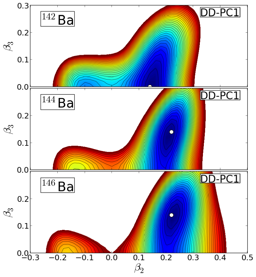
Figure 1: (Color online) The SCMF ($\beta_{2},\beta_{3}$) deformation energy surfaces for ^142,144,146Ba, obtained with the DD-PC1 nuclear functional Nikšić et al. (2008) and a separable pairing force of finite range Tian et al. (2009). The energy difference between neighbouring contours is 200 keV. Equilibrium minima are identified by open circles.

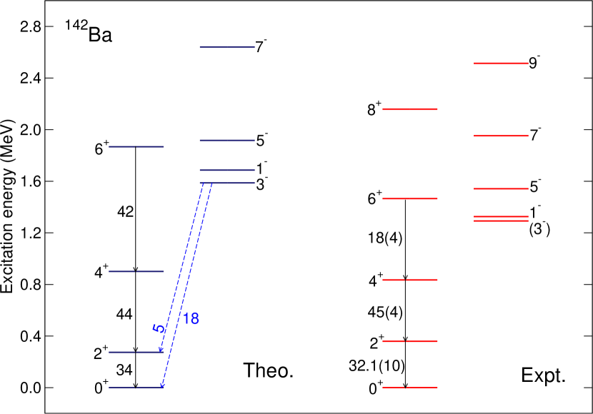
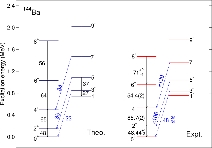
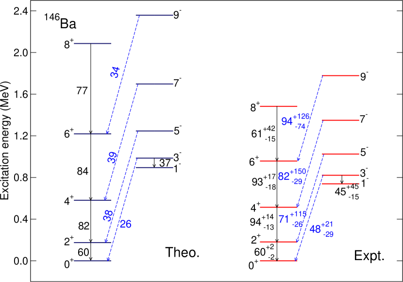
Figure 2: (Color online) Low-energy positive- and negative-parity spectra of the even-even boson core nuclei ^142,144,146Ba. The $B(E2)$ (numbers along arrows within each band) and $B(E3)$ (inter-band, dashed arrows) values are given in Weisskopf units. Experimental values are taken from Ref. Brookhaven National Nuclear Data Center (¹⁴²Ba), Ref. Bucher et al. (2016) (¹⁴⁴Ba) and Ref. Bucher et al. (2017) (¹⁴⁶Ba).

We first briefly discuss the results obtained for the even-even nuclei ^142,144,146Ba. Figure 1 depicts the axially-symmetric ($\beta_{2},\beta_{3}$) deformation energy surfaces calculated with the constrained relativistic Hartree-Bogoliubov method. For ¹⁴²Ba the equilibrium minimum is found on the $\beta_{3}=0$ axis, indicating that it has a weakly-deformed quadrupole shape. In ^144,146Ba a minimum with non-zero $\beta_{3}$ deformation ($\beta\approx 0.1$) appears. The minimum is not very pronounced and is rather soft in the $\beta_{3}$ direction, suggesting the occurrence of octupole vibrational states in these nuclei.

The excitation spectra and transition rates for ^142,144,146Ba are computed by diagonalizing the IBM Hamiltonian Eq. (3), determined from the SCMF ($\beta_{2},\beta_{3}$) deformation energy surface, in the $sdf$-boson basis. The low-energy level schemes for the ^142,144,146Ba isotopes are displayed in Fig. 2. In general, the theoretical predictions are in good agreement with the experimental results Brookhaven National Nuclear Data Center ; Bucher et al. (2016, 2017), not only for the excitation energies but also for the $E2$ and $E3$ transition strengths. In the transition from ¹⁴²Ba ¹⁴⁴Ba nucleus, in particular, we note the pronounced lowering of the the negative-parity band (cf. the corresponding SCMF deformation energy surface in Fig. 1). A rather large value $B(E3;3^{-}\rightarrow 0^{+})$ is predicted for all three even-even Ba nuclei, but still considerably smaller than the experimental values reported for ^144,146Ba Bucher et al. (2016, 2017). Note, however, the large uncertainty of the latter.

IV Spectroscopic properties of odd-mass Ba isotopes

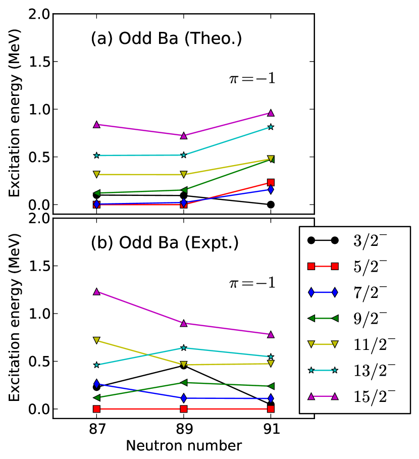
Figure 3: (Color online) Evolution of low-energy negative-parity levels of the odd-mass Ba isotopes as functions of the neutron number. Experimental excitation energies are taken from Refs. Zhu et al. (1999); Rzaca-Urban et al. (2012, 2013).

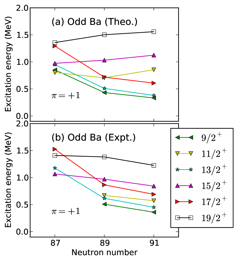
Figure 4: (Color online) Same as Fig. 3, but for the positive-parity levels.

IV.1 Evolution of low-energy excitation spectra

In Figs. 3 and 4 the lowest-energy negative- and positive-parity states for for each spin of ^143,145,147Ba are plotted as functions of the neutron number, respectively. Note that the spin and parity of the lowest ${3/2}^{-}$ state for ¹⁴³Ba, the ${3/2}^{-}$, ${11/2}^{+}$, ${15/2}^{+}$, ${19/2}^{+}$ states for ¹⁴⁵Ba, and the ${3/2}^{-}$, ${11/2}^{-}$, ${15/2}^{-}$, ${11/2}^{+}$, ${15/2}^{+}$ and ${19/2}^{+}$ states have been assigned tentatively Zhu et al. (1999); Rzaca-Urban et al. (2012, 2013); Brookhaven National Nuclear Data Center . The excitation spectra obtained by the diagonalization of the $sdf$-IBFM Hamiltonian reproduce the trend of the data, even though very little variation has been allowed for most of the strength parameters for the boson-fermion interaction (Table 3). In ¹⁴⁷Ba, however, experimentally the spin of the ground state is $J^{\pi}={5/2}^{-}$ Rzaca-Urban et al. (2013), whereas in the present calculation it is $J^{\pi}={3/2}^{-}$. This state could be among the lowest in the data on ¹⁴⁷Ba. A signature of shape transition is a rather rapid decrease of the ${9/2}^{+}$, ${13/2}^{+}$ and ${17/2}^{+}$ energy levels from ¹⁴³Ba to ¹⁴⁵Ba, and somewhat less steep from ¹⁴⁵Ba to ¹⁴⁷Ba. The empirical trend is nicely reproduced by the calculation, and this correlates with the fact that, in the even-even systems, the non-zero octupole equilibrium deformation $\beta_{3}$ appears in the SCMF energy surface for ¹⁴⁴Ba (Fig. 1). There are no distinct irregularities in the excitation spectra shown in Figs. 3 and 4.

IV.2 Detailed comparison of level schemes

Figures 5–7 display detailed comparisons between theoretical and experimental positive-parity and negative-parity low-lying bands in the odd-mass nuclei ^143,145,147Ba. In organizing the theoretical level schemes, states are classified into bands according to the dominant E2 decay rates and the similarity in the composition of their IBFM wave functions. The labels in parentheses denote states that are assigned only tentatively in experiment. Also, only experimental states that are classified into bands are plotted in Figs. 5–7. Some experimental states that do not belong to these bands, for instance the ${3/2}^{-}_{1}$ and ${7/2}^{-}_{1}$ states for ¹⁴³Ba, are not included in Fig. 5, even though they are plotted in Fig. 3. In Tables 5–9 we list the expectation values of the $f$-boson number operator $\langle\hat{n}_{f}\rangle$, as well as the contribution of each single-particle component in the IBFM wave function of the band-head state of each band. The predicted $B(E2)$ and $B(E3)$ values are included in Tables 6–8. Note that presently data are not available for these quantities.

IV.2.1 ¹⁴³Ba

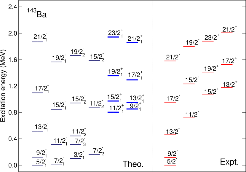
Figure 5: (Color online) Detailed comparison of the calculated and experimental low-energy positive- and negative-parity spectra of ¹⁴³Ba. Those theoretical energy levels that are made of one $f$-boson configuration are drawn in bold and in color blue. Data are taken from Ref. Rzaca-Urban et al. (2012).

For the even-even core nucleus ¹⁴²Ba the SCMF ($\beta_{2},\beta_{3}$) deformation energy surface exhibits an equilibrium minimum at axial quadrupole deformation $\beta_{2}\approx 0.14$ and octupole deformation $\beta_{3}=0$, and the corresponding spectra display negative-parity states at relatively high excitation energies compared to ^144,146Ba. Hence, octupole deformation is expected to play a rather minor role in the odd-mass system ¹⁴³Ba. Experimentally four bands, two of positive- and two negative-parity each, have been established in ¹⁴³Ba Zhu et al. (1999). The predicted level scheme shown in Fig. 5 reproduces nicely the lowest negative-parity ground-state band built on the ${5/2}^{-}_{1}$ state, as well as the energy of the ${15/2}^{+}_{1}$ state, which is the lowest positive-party state in experiment.

As shown in Table 5, the present calculation does not predict the presence of octupole states (i.e., states that contain one or more $f$ bosons in their wave functions) in the vicinity of the ground state in ¹⁴³Ba: all the negative-parity bands shown in Fig. 5 are composed mainly of the odd neutron in the $pfh$ orbitals coupled to the $sd$-boson space. On the other hand, the band built on the $11/2^{+}_{1}$ state is predicted to contain predominantly states with one $f$-boson, and similar for the ${9/2}^{+}_{1}$ band. From Table 4 one notices several significant $B(E3)$ transition probabilities from the bands based on the $J^{\pi}={9/2}^{+}_{1}$ and $11/2^{+}_{1}$ states to the low-lying decoupled negative-parity band, e.g., $B(E3;{15/2}^{+}_{1}\rightarrow{9/2}^{-}_{1})=11$ W.u. and $B(E3;{17/2}^{+}_{1}\rightarrow{11/2}^{-}_{1})=13$ W.u.

Table 4: Predicted $B(E2)$ and $B(E3)$ values (in Weisskopf units) for transitions among low-energy states of ¹⁴³Ba.

$B(E\lambda;J_{i}^{\pi}\rightarrow J_{f}^{\pi})$	Theory (W.u.)
$B(E2;{9/2}^{-}_{1}\rightarrow{5/2}^{-}_{1})$	16
$B(E2;{11/2}^{-}_{1}\rightarrow{7/2}^{-}_{1})$	25
$B(E2;{13/2}^{-}_{1}\rightarrow{9/2}^{-}_{1})$	35
$B(E2;{13/2}^{+}_{1}\rightarrow{9/2}^{+}_{1})$	21
$B(E2;{15/2}^{+}_{1}\rightarrow{11/2}^{+}_{1})$	31
$B(E2;{11/2}^{+}_{2}\rightarrow{7/2}^{+}_{1})$	4.2
$B(E3;{11/2}^{+}_{1}\rightarrow{5/2}^{-}_{1})$	5.5
$B(E3;{15/2}^{+}_{1}\rightarrow{9/2}^{-}_{1})$	11
$B(E3;{13/2}^{+}_{1}\rightarrow{7/2}^{-}_{1})$	8.4
$B(E3;{17/2}^{+}_{1}\rightarrow{11/2}^{-}_{1})$	13

Table 5: Expectation value of the $f$-boson number operator $\langle\hat{n}_{f}\rangle$, and squares of the amplitudes (in percentage) of each spherical single-particle configuration in the IBFM wave functions of band-head states in ¹⁴³Ba (cf. Fig. 5.)

$J^{\pi}$	$\langle\hat{n}_{f}\rangle$	$3p_{1/2}$	$3p_{3/2}$	$2f_{5/2}$	$2f_{7/2}$	$1h_{9/2}$	$1i_{13/2}$
${5/2}^{-}_{1}$	0.000	0	0	4	4	92	0
${7/2}^{-}_{1}$	0.000	0	0	2	5	93	0
${3/2}^{-}_{1}$	0.000	0	9	0	78	13	0
${7/2}^{-}_{2}$	0.001	0	9	0	80	11	0
${11/2}^{+}_{1}$	1.000	0	0	2	2	96	0
${9/2}^{+}_{1}$	1.000	0	0	2	3	95	0

IV.2.2 ¹⁴⁵Ba

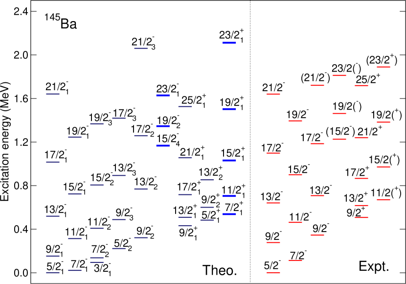
Figure 6: (Color online) Same as in the caption to Fig. 5, but for the nucleus ¹⁴⁵Ba. Experimental excitation energies are from Ref. Rzaca-Urban et al. (2012).

More experimental information is available on the isotope ¹⁴⁵Ba and, as discussed in Sec. III, since the corresponding even-even boson core nucleus ¹⁴⁴Ba exhibits an octupole-soft potential at the SCMF level (cf. Fig. 1), we also expect that octupole correlations play a more important role in the low-energy spectra of this nucleus. The calculated excitation spectrum is compared to the corresponding experimental bands in Fig. 6. As shown in Table 7, the lowest two negative-parity bands in ¹⁴⁵Ba are built on the ${5/2}^{-}_{1}$ and ${7/2}^{-}_{1}$ states that are characterized by the coupling of the unpaired neutron in the $1h_{9/2}$ single-particle orbital to the $sd$ boson space. The lowest positive-parity state ${9/2}^{+}_{1}$ is described by the coupling of the $1i_{13/2}$ orbital to $sd$-boson states.

From Table 7 it follows that the theoretical negative-parity band built on the ${15/2}^{-}_{4}$ state (calculated at 1167 keV) is dominated by the coupling of the $1i_{13/2}$ single-particle orbital to states with one $f$-boson. Theoretically the ${15/2}^{-}_{4}$ state appears to be an octupole state and is located close to the experimental ${15/2}^{-}$ state found at 1226 keV Rzaca-Urban et al. (2012). Moreover, rather strong E3 transitions from the $J^{\pi}={15/2}^{-}_{4}$ band to the corresponding low-lying positive-parity bands are predicted: for instance $B(E3;{15/2^{-}_{4}}\rightarrow{9/2^{+}_{1}})=25$ and $B(E3;{19/2^{-}_{2}}\rightarrow{13/2^{+}_{1}})=31$ (in W.u), comparable to the $B(E3;3^{-}_{1}\rightarrow 0^{+}_{1})$ value of 23 W.u. in the corresponding even-even core nucleus ¹⁴⁴Ba (see, Fig. 2). However, to verify model predictions, experimental information on the $B(E2)$ and $B(E3)$ values is needed.

For positive parity, the theoretical band built on the ${7/2}^{+}_{1}$ in ¹⁴⁵Ba corresponds to the coupling of the $1h_{9/2}$ single-neutron configuration to states with one $f$-boson (cf. Table 7). The theoretical ${11/2}^{+}_{1}$ level, calculated at 705 keV, can be compared with the experimental ${11/2}^{+}$ state at 670 keV Rzaca-Urban et al. (2012), which has been suggested as a candidate for an octupole state. Non-negligible E3 transition strength from the ${7/2}^{+}_{1}$ band to the negative-parity ground-state band is predicted in the present calculation: $B(E3;{11/2^{+}_{1}}\rightarrow{5/2^{-}_{1}})=4.7$ and $B(E3;{15/2^{+}_{1}}\rightarrow{9/2^{-}_{1}})=15$ (in W.u).

Table 6: Same as in the caption to Table 4, but for the ¹⁴⁵Ba nucleus.

$B(E\lambda;J_{i}^{\pi}\rightarrow J_{f}^{\pi}$)	Theory (W.u.)
$B(E2;{7/2}^{-}_{1}\rightarrow{5/2}^{-}_{1})$	23
$B(E2;{9/2}^{-}_{1}\rightarrow{5/2}^{-}_{1})$	10
$B(E2;{11/2}^{-}_{1}\rightarrow{7/2}^{-}_{1})$	23
$B(E2;{13/2}^{-}_{1}\rightarrow{9/2}^{-}_{1})$	38
$B(E2;{11/2}^{+}_{1}\rightarrow{7/2}^{+}_{1})$	21
$B(E2;{13/2}^{+}_{1}\rightarrow{9/2}^{+}_{1})$	75
$B(E2;{15/2}^{+}_{1}\rightarrow{11/2}^{+}_{1})$	43
$B(E2;{17/2}^{+}_{1}\rightarrow{13/2}^{+}_{1})$	78
$B(E3;{11/2}^{+}_{1}\rightarrow{5/2}^{-}_{1})$	4.7
$B(E3;{15/2}^{+}_{1}\rightarrow{9/2}^{-}_{1})$	15
$B(E3;{13/2}^{+}_{1}\rightarrow{7/2}^{-}_{1})$	0.028
$B(E3;{17/2}^{+}_{1}\rightarrow{11/2}^{-}_{1})$	0.59
$B(E3;{15/2}^{-}_{1}\rightarrow{9/2}^{+}_{1})$	0.00014
$B(E3;{15/2}^{-}_{2}\rightarrow{9/2}^{+}_{1})$	0.00078
$B(E3;{15/2}^{-}_{4}\rightarrow{9/2}^{+}_{1})$	25
$B(E3;{19/2}^{-}_{2}\rightarrow{13/2}^{+}_{1})$	31

Table 7: Same as in the caption to Table 5, but for ¹⁴⁵Ba.

$J^{\pi}$	$\langle\hat{n}_{f}\rangle$	$3p_{1/2}$	$3p_{3/2}$	$2f_{5/2}$	$2f_{7/2}$	$1h_{9/2}$	$1i_{13/2}$
${5/2}^{-}_{1}$	0.000	0	0	5	3	92	0
${7/2}^{-}_{1}$	0.000	0	0	1	4	95	0
${3/2}^{-}_{1}$	0.005	3	17	1	67	11	0
${5/2}^{-}_{2}$	0.002	1	9	1	70	20	0
${9/2}^{-}_{2}$	0.000	0	1	2	8	89	0
${15/2}^{-}_{4}$	0.998	0	0	0	0	0	100
${9/2}^{+}_{1}$	0.000	0	0	0	0	0	100
${5/2}^{+}_{1}$	0.005	0	0	0	0	0	99
${7/2}^{+}_{1}$	1.000	0	0	1	4	95	0

IV.2.3 ¹⁴⁷Ba

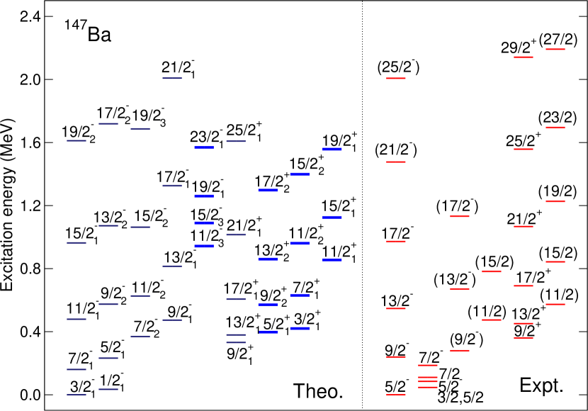
Figure 7: (Color online) Same as in the caption to Fig. 5, but for ¹⁴⁷Ba and with data from Ref. Rzaca-Urban et al. (2013).

From the SCMF ($\beta_{2},\beta_{3}$) deformation energy surfaces of ¹⁴⁴Ba and ¹⁴⁶Ba (cf. Fig. 1) one expects rather similar low-energy excitation spectra in their odd-$N$ neighbours ¹⁴⁵Ba and ¹⁴⁷Ba, respectively. This is, to a certain extent, observed in the experimental spectra Rzaca-Urban et al. (2013), even though the bands of ¹⁴⁷Ba appear more compressed, as seen when comparing the data in Figs. 6 and 7. The ground-state spin ${5/2}^{-}$ has been identified for ¹⁴⁷Ba, just as in the ^143,145Ba neighbours Rzaca-Urban et al. (2013). This is, however, at variance within the present calculation, which predicts ${3/2}^{-}$ for the ground state. In fact, it is possible to reproduce the ground state spin of $J={5/2}^{-}$ by playing with the parameters. In that case, however, one would have to choose an unrealistic value for the boson-fermion interaction strength, for instance, negative value for $\Gamma^{(sd)}_{0}$. The wrong sign implies that the single-particle energies and/or occupation probabilities used in the present calculation are not necessarily optimal. We then checked that decreasing the occupation probability for the $1h_{9/2}$ orbital, for instance, by 25 %, allowed to reproduce the correct level ordering of the ground state, but such an adjustment is not justified within the present framework and is beyond the scope of this paper. Nevertheless, one notices in Fig. 7 that a low-lying $J={3/2}$ level could be also present in experiment Rzaca-Urban et al. (2013), i.e., among a set of levels close to the $J^{\pi}={5/2}^{-}$ ground state, even though its spin and parity have not been firmly established. Table 9 also shows that the structure of the IBFM wave functions of the lowest-lying states in ¹⁴⁷Ba is different from those for ^143,145Ba: they are dominated by the $1h_{9/2}$ configuration in ^143,145Ba, whereas in ¹⁴⁷Ba low-energy negative parity states are characterized by the mixing of the $3p_{1/2,3/2}2f_{5/2,7/2}$ single-particle configurations.

One also notices from Table 9 that states in the lowest two bands, built on the ${3/2}^{-}_{1}$ and ${1/2}^{-}_{1}$, do not contain $f$-boson components in their wave functions. The negative-parity bands built on the ${7/2}^{-}_{2}$ and ${9/2}^{-}_{1}$ states predominantly correspond to the $1h_{9/2}$ configuration coupled with the $sd$-boson space, and again there is no octupole $f$-boson component in these bands. The calculation predicts the lowest negative-parity octupole band to be the one built on the ${11/2}^{-}_{3}$ state, and this band is connected by rather strong E3 transition to the ground state band, e.g., $B(E3;{15/2}^{-}_{3}\rightarrow{9/2}^{+}_{1})=29$ W.u. The experimental band built on the ${11/2}$ state at 573 keV (with tentative assignment of positive parity) has been identified as a possible octupole structure Rzaca-Urban et al. (2013). This band can be compared to the theoretical sequence with the ${11/2}^{+}_{1}$ band-head at excitation energy 855 keV, dominated by the $1h_{9/2}$ single-particle orbital coupled to the $sdf$-boson space.

Table 8: Same as in the caption to Table 4, but for the ¹⁴⁷Ba nucleus.

$B(E\lambda;J_{i}^{\pi}\rightarrow J_{f}^{\pi}$)	Theory (W.u.)
$B(E2;{7/2}^{-}_{1}\rightarrow{5/2}^{-}_{1})$	13
$B(E2;{9/2}^{-}_{1}\rightarrow{5/2}^{-}_{1})$	0.89
$B(E2;{9/2}^{-}_{2}\rightarrow{5/2}^{-}_{1})$	104
$B(E2;{11/2}^{-}_{2}\rightarrow{7/2}^{-}_{2})$	24
$B(E2;{13/2}^{-}_{1}\rightarrow{9/2}^{-}_{1})$	44
$B(E2;{11/2}^{+}_{1}\rightarrow{7/2}^{+}_{1})$	0.17
$B(E2;{13/2}^{+}_{1}\rightarrow{9/2}^{+}_{1})$	92
$B(E2;{15/2}^{+}_{1}\rightarrow{11/2}^{+}_{1})$	48
$B(E2;{17/2}^{+}_{1}\rightarrow{13/2}^{+}_{1})$	97
$B(E3;{11/2}^{+}_{1}\rightarrow{5/2}^{-}_{1})$	0.037
$B(E3;{11/2}^{+}_{2}\rightarrow{5/2}^{-}_{1})$	25
$B(E3;{15/2}^{+}_{1}\rightarrow{9/2}^{-}_{1})$	15
$B(E3;{15/2}^{-}_{3}\rightarrow{9/2}^{+}_{1})$	29
$B(E3;{19/2}^{-}_{1}\rightarrow{13/2}^{+}_{1})$	38

Table 9: Same as in the caption to Table 5, but for ¹⁴⁷Ba.

$J^{\pi}$	$\langle\hat{n}_{f}\rangle$	$3p_{1/2}$	$3p_{3/2}$	$2f_{5/2}$	$2f_{7/2}$	$1h_{9/2}$	$1i_{13/2}$
${3/2}^{-}_{1}$	0.002	14	38	9	39	0	0
${1/2}^{-}_{1}$	0.000	20	35	17	28	0	0
${7/2}^{-}_{2}$	0.000	0	0	0	2	98	0
${9/2}^{-}_{1}$	0.000	0	0	1	2	97	0
${11/2}^{-}_{3}$	0.996	0	0	0	0	0	100
${9/2}^{+}_{1}$	0.002	0	0	0	0	0	100
${5/2}^{+}_{1}$	0.950	10	31	8	45	0	6
${3/2}^{+}_{1}$	0.999	14	33	15	35	3	0
${11/2}^{+}_{1}$	1.000	0	0	1	2	97	0

V Conclusions

The role of octupole correlations and the relevant spectroscopic properties of neutron-rich odd-mass Ba isotopes have been analyzed in a theoretical framework based on nuclear density functional theory and the particle-core coupling scheme. In the particular method employed in the present study, the interacting-boson Hamiltonian that describes the even-even core nucleus, as well as the single-particle energies and occupation probabilities of an unpaired nucleon, are completely determined by constrained SCMF calculations for a given choice of the energy density functional and pairing interaction. Only the coupling constants for the boson-fermion interaction are adjusted to selected spectroscopic data for the low-lying states in the odd-mass systems.

In this work the $sdf$-IBFM framework has been implemented: the boson-core Hamiltonian involves both quadrupole and octupole boson degrees of freedom and is constructed fully microscopically by mapping the axially-symmetric ($\beta_{2},\beta_{3}$) deformation energy surface obtained by a constrained relativistic Hartree-Bogoliubov SCMF calculation onto the expectation value of the Hamiltonian in the $sdf$-boson condensate state. In the odd-mass Ba nuclei considered here the role of octupole deformation is not very important for the lowest levels near the ground state, and the adjustment of the boson-fermion strength parameters is relatively straightforward, even though there are many terms in the corresponding Hamiltonian Eq. (6).

The SCMF ($\beta_{2},\beta_{3}$) deformation energy surfaces for the even-even Ba nuclei exhibit a transition from a weakly deformed quadrupole shape of ¹⁴²Ba to moderately quadrupole and octupole deformed shapes of ^144,146Ba, characterized by $\beta_{3}$-soft potentials. The resulting $sdf$ IBM energy spectra display a signature of octupole collectivity in the pronounced E3 transitions between the low-lying negative-parity band and the ground-state band, in agreement with recent spectroscopic data Bucher et al. (2016, 2017). The $sdf$-IBFM reproduces the experimental low-energy excitation spectra in the considered odd-mass Ba isotopes fairly well. In particular, the present calculation indicates that octupole correlations are not present in the lowest states of ^143,145,147Ba nuclei: most of their low-lying positive- and negative-parity yrast bands are predominantly formed by coupling the odd-neutron orbitals to the $sd$ boson space. Octupole states have been identified at somewhat higher excitation energy – e.g., in ¹⁴⁵Ba the bands built on the ${15/2}^{-}_{4}$ and ${7/2}^{+}_{1}$ states are characterized by the coupling of the odd-neutron to the $sd+f$ boson space, and exhibit pronounced E3 transitions to the ground state band. These results, especially for ^145,147Ba, are consistent with the conclusion of recent experimental studies Rzaca-Urban et al. (2012, 2013).

A particularly interesting case for a follow-up study are spectroscopic properties of actinide nuclei, e.g., ^224,225Ra, where signatures of stable octupole shapes have been suggested and identified experimentally, such as parity doublets, pronounced electric dipole and octupole transitions. The low-energy states of these actinide nuclei are much richer in structure compared to the present case, as octupole correlations are expected to be as prominent as the quadrupole ones. A quantitative analysis of quadrupole and octupole degrees of freedom in odd-mass nuclei in this region certainly presents a challenging application of the method introduced in the present work.