Distributed Convergence Verification for Gaussian Belief Propagation

Abstract

Gaussian belief propagation (BP) is a computationally efficient method to approximate the marginal distribution and has been widely used for inference with high dimensional data as well as distributed estimation in large-scale networks. However, the convergence of Gaussian BP is still an open issue. Though sufficient convergence conditions have been studied in the literature, verifying these conditions requires gathering all the information over the whole network, which defeats the main advantage of distributed computing by using Gaussian BP. In this paper, we propose a novel sufficient convergence condition for Gaussian BP that applies to both the pairwise linear Gaussian model and to Gaussian Markov random fields. We show analytically that this sufficient convergence condition can be easily verified in a distributed way that satisfies the network topology constraint.

Index Terms—  graphical model, belief propagation, large-scale networks, distributed inference, Markov random field.

1 Introduction

Gaussian belief propagation (BP) [1, 2] provides an efficiently distributed way to compute the marginal distribution of unknown variables with a joint Gaussian distribution, and Gaussian BP has been adopted in a variety of topics including image denosing [3], distributed power state estimation [4] in smart grid, data detection for massive MIMO systems[5], distributed beamforming [6] and synchronization [7, 8, 9, 10] in distributed networks, fast solver for system of linear equations [11], distributed rate control in ad-hoc networks [12], factor analyzer networks [13], sparse Bayesian learning [14], inter-cell interference mitigation [15], and peer-to-peer rating in social networks [16]. It has been shown that Gaussian BP computes the optimal centralized estimator if it converges [1, 2]. The challenge of deploying Gaussian BP for large-scale networks is determining if it will converge. In particular, it is generally known that, if the factor graph, which represents the joint distribution, contains cycles, the Gaussian BP algorithm may diverge. Thus, determining convergence conditions for the Gaussian BP algorithm is very important. Further, in practical applications for large-scale networks, having an easily verified sufficient convergence condition is of great importance.

Sufficient convergence conditions for Gaussian BP have been developed in [17, 2, 18] when the underlying Gaussian distribution is expressed in terms of Gaussian Markov random fields (GMRFs) with scalar variables. These works focus on the convergence analysis of Gaussian BP for computing the marginal distribution of a joint distribution with pairwise factors. However, as demonstrated in [1], the iterative equations for Gaussian BP on GMRFs are different from those for distributed estimation problems such as in [4, 6, 7, 8, 11, 12, 13, 14, 15], where linear Gaussian measurements are involved.

Recently, the convergence properties of Gaussian BP for the linear Gaussian measurement model with vector variables have been studied in [1]. It is analytically shown that the marginal covariance for each unknown vector variable converges to a unique positive definite matrix with double exponential rate with arbitrary positive-semidefinite initial message information matrix. Further, a sufficient convergence condition that guarantees the belief mean to converge to the exact marginal mean is also given. It is also shown that this sufficient convergence condition subsumes all the previous sufficient convergence conditions in [17, 2, 18].

Though sufficient convergence conditions have been studied for both the GMRFs and linear Gaussian models, verifying these conditions all require to gather all the information together to perform centralized computation. For example, in [1], the convergence condition requires computation with complexity of $\mathcal{O}(N^{3})$ of the spectrum radius of a dimension-$N$ matrix, where $N$ is the dimension of a vector constructed by stacking together all the mean vectors exchanged in the network at each iteration. This defeats the main advantage of low computation complexity of a distributed inference algorithm. In this paper, we present a sufficient convergence condition for Gaussian BP on both GMRFs and linear Gaussian models and demonstrate that it can be easily verified in a distributed way that respects the network topology constraints.

2 Computation Model

2.1 Belief Propagation

The BP algorithm computes the marginal distribution/function given a factorization of the distribution/function. The factorization can be represented by a graphical model known as factor graph [19], and the BP algorithm can be expressed as message passing on the factor graph.

In the factor graph, every vector variable $\textbf{x}_{i}$ is represented by a circle (called variable node) and the probability distribution of a vector variable or a group of vector variables is represented by a square (called factor node). A variable node is connected to a factor node if the variable is involved in that particular factor. For example, Fig. 1 shows the factor graph representation of a joint Gaussian distribution. The explicit functions of $f_{i,j}$ and $f_{i}$ for the linear Gaussian model and the GMRF will be given later.

We next derive the BP algorithm over the corresponding factor graph. It involves two types of messages: one is the message from a variable node $\textbf{x}_{j}$ to its neighboring factor node $f_{i,j}$, defined as

$$m^{\left(\ell\right)}_{j\to f_{i,j}}\left(\textbf{x}_{j}\right)=p\left(\textbf{x}_{j}\right)\prod_{f_{k,j}\in\mathcal{B}(j)\setminus f_{i,j}}m^{\left(\ell-1\right)}_{f_{k,j}\to j}\left(\textbf{x}_{j}\right),$$ (1)

where $\mathcal{B}\left(j\right)$ denotes the set of neighbouring factor nodes of $\textbf{x}_{j}$, and $m^{\left(\ell-1\right)}_{f_{k,j}\to j}\left(\textbf{x}_{j}\right)$ is the message from $f_{k,j}$ to $\textbf{x}_{j}$ at iteration $\ell-1$. The second type of message is from a factor node $f_{i,j}$ to a neighboring variable node $\textbf{x}_{i}$, defined as

$$m^{\left(\ell\right)}_{f_{i,j}\to i}\left(\textbf{x}_{i}\right)=\int\!\!\!\cdots\!\!\!\int f_{i,j}\times\!\!\!\!\!\prod_{j\in\mathcal{B}\left(f_{i,j}\right)\setminus i}\!\!\!\!\!\!\!m^{\left(\ell\right)}_{j\to f_{i,j}}\left(\textbf{x}_{j}\right)\,\!\!\mathrm{d}\left\{\textbf{x}_{j}\right\}_{j\in{\mathcal{B}}\left(f_{i,j}\right)\setminus i},$$ (2)

where $\mathcal{B}\left(f_{i,j}\right)$ denotes the set of neighboring variable nodes of $f_{i,j}$. The process iterates between equations (1) and (2). At each iteration $\ell$, the approximate marginal distribution, also referred to as belief, on $\textbf{x}_{i}$ is computed locally at $\textbf{x}_{i}$ as

$$b_{\textrm{BP}}^{\left(\ell\right)}\left(\textbf{x}_{i}\right)=p\left(\textbf{x}_{i}\right)\prod_{f_{n}\in\mathcal{B}\left(i\right)}m^{\left(\ell\right)}_{f_{n}\to i}\left(\textbf{x}_{i}\right).$$ (3)

In the following subsections, we show the updating equations of Gaussian BP for the linear Gaussian model and the GMRF.

2.2 Linear Gaussian Model

Consider a general connected network of $M$ nodes, with $\mathcal{V}=\{1,\ldots,M\}$ denoting the set of nodes, and $\mathcal{E}_{\textrm{Net}}\subset\mathcal{V}\times\mathcal{V}$ the set of all undirect communication links in the network, i.e., if $i$ and $j$ are within the communication range, $(i,j)\in\mathcal{E}_{\textrm{Net}}$. The local observations, $\textbf{y}_{i,j}$, between node $i$ and $j$ are modeled by the pairwise linear Gaussian model [20, 21]:

$$\textbf{y}_{i,j}=\textbf{A}_{j,i}\textbf{x}_{i}+\textbf{A}_{i,j}\textbf{x}_{j}+\textbf{z}_{i,j},$$ (4)

where $\textbf{A}_{j,i}$ and $\textbf{A}_{i,j}$ are known coefficient matrices with full column rank, $\textbf{x}_{i}$ and $\textbf{x}_{j}$ are local unknown vector parameters at node $i$ and $j$ with dimension $N_{i}\times 1$ and $N_{j}\times 1$, and with prior distribution $p(\textbf{x}_{i})\sim\mathcal{N}(\textbf{x}_{i}|\textbf{0},\textbf{W}_{i})$ and $p(\textbf{x}_{j})\sim\mathcal{N}(\textbf{x}_{j}|\textbf{0},\textbf{W}_{j})$, and $\textbf{z}_{i,j}$ is additive noise with distribution $\textbf{z}_{i,j}\sim\mathcal{N}(\textbf{z}_{i,j}|\textbf{0},\textbf{R}_{i,j})$. It is assumed that $p(\textbf{x}_{i},\textbf{x}_{j})=p(\textbf{x}_{i})p(\textbf{x}_{j})$ and $p(\textbf{z}_{i,j},\textbf{z}_{s,t})=p(\textbf{z}_{i,j})p(\textbf{z}_{s,t})$ for $\{i,j\}\neq\{s,t\}$. The goal is to estimate $\textbf{x}_{i}$, based on $\textbf{y}_{i,j}$, $p(\textbf{x}_{i})$ and $p(\textbf{z}_{i,j})$ for all $\textbf{x}_{i}\in\mathcal{V}$. Note that in (4), $\textbf{y}_{i,j}=\textbf{y}_{j,i}$.

The joint distribution $p\left(\textbf{x}\right)p\left(\textbf{y}|\textbf{x}\right)$ is first written as the product of the prior distribution and the likelihood function as

$$p\left(\textbf{x}\right)p\left(\textbf{y}|\textbf{x}\right)=\prod_{i\in\mathcal{V}}\underbrace{p\left(\textbf{x}_{i}\right)}_{\triangleq g_{i}}\prod_{i\in\mathcal{V}}\underbrace{p(\textbf{y}_{i,j}|\textbf{x}_{i},\textbf{x}_{j},\{i,j\}\in\mathcal{E}_{\textrm{Net}})}_{\triangleq g_{i,j}}.$$ (5)

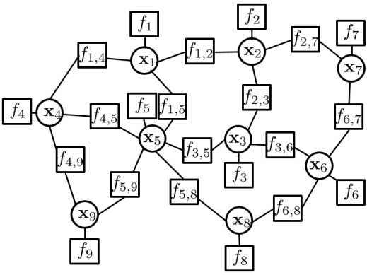
Fig. 1: An example of factor graph representing a joint Gaussian distribution.

Following the computation rule of (2), it can be easily shown that the message from a factor that denotes prior information is a constant, i.e., $m^{(\ell)}_{{f}_{i}\to i}(\textbf{x}_{i})=p(\textbf{x}_{i}),\quad\forall\ell=0,1,\ldots.$ Further, from (2) and (1), message $m^{(\ell)}_{i\to f_{i}}(\textbf{x}_{i})$ will never be used for message updating. Therefore, we next focus on the message exchange between the factor denoting the likelihood function and its neighboring variables.

It can be shown that the message from a factor node to a variable node is given by [1]

$$m^{(\ell)}_{f_{i,j}\to i}(\textbf{x}_{i})\propto\exp\big{\{}-\frac{1}{2}||\textbf{x}_{i}-\textbf{v}^{(\ell)}_{f_{i,j}\to i}||_{\textbf{C}^{(\ell)}_{f_{i,j}\to i}}\big{\}},$$ (6)

where $\textbf{C}_{f_{i,j}\to i}^{(\ell-1)}$ and $\textbf{v}_{f_{i,j}\to i}^{(\ell-1)}$ are the message covariance matrix and mean vector received at variable node $i$ at the $\ell-1$ iteration with

$$\begin{split}\left[\textbf{C}^{(\ell)}_{f_{i,j}\to i}\right]^{-1}=\textbf{A}_{j,i}^{T}\left[\textbf{R}_{i,j}+\textbf{A}_{i,j}\textbf{C}^{(\ell)}_{j\to f_{i,j}}\textbf{A}_{i,j}^{T}\right]^{-1}\textbf{A}_{j,i}.\end{split}$$ (7)

and

$$\begin{split}\textbf{v}^{(\ell)}_{f_{i,j}\to i}=&\textbf{A}_{j,i}^{T}\left[\textbf{R}_{i,j}+\textbf{A}_{i,j}\textbf{C}^{(\ell)}_{j\to f_{i,j}}\textbf{A}_{i,j}^{T}\right]^{-1}\\ &\times\left(\textbf{y}_{i,j}-\textbf{A}_{i,j}\textbf{v}^{(\ell)}_{j\to f_{i,j}}\right).\end{split}$$ (8)

Furthermore, the general expression for the message from a variable node to a factor node is

$$m^{(\ell)}_{j\to f_{i,j}}(\textbf{x}_{j})\propto\exp\left\{-\frac{1}{2}||\textbf{x}_{j}-\textbf{v}^{(\ell)}_{j\to f_{i,j}}||_{\textbf{C}^{(\ell)}_{j\to f_{i,j}}}\right\},$$ (9)

where $\textbf{C}_{j\to f_{i,j}}^{(\ell)}$ and $\textbf{v}_{j\to f_{i,j}}^{(\ell)}$ are the message covariance matrix and mean vector received at variable node $j$ at the $\ell$-th iteration, where the inverse of the covariance matrix updating equation is given by

$$\big{[}\textbf{C}^{(\ell)}_{j\to f_{i,j}}\big{]}^{-1}=\textbf{W}_{j}^{-1}+\sum_{f_{k,j}\in{\mathcal{B}}(j)\setminus f_{i,j}}\big{[}\textbf{C}_{f_{k,j}\to j}^{(\ell-1)}\big{]}^{-1},$$ (10)

and the mean vector is

$$\textbf{v}^{(\ell)}_{j\to f_{i,j}}=\textbf{C}^{(\ell)}_{j\to f_{i,j}}\bigg{[}\sum_{f_{k,j}\in{\mathcal{B}}(j)\setminus f_{i,j}}\big{[}\textbf{C}_{f_{k,j}\to j}^{(\ell-1)}\big{]}^{-1}\textbf{v}^{(\ell-1)}_{f_{k,j}\to j}\bigg{]}.$$ (11)

Following Lemma 2 in [1], we know that setting the initial message covariances inverse (also known as the message information matrix) $[\textbf{C}_{f_{k,j}\to i}^{(0)}]^{-1}\succeq\textbf{0}$ for all $k\in\mathcal{V}$ and $j\in\mathcal{B}(k)$ guarantees $[\textbf{C}^{(\ell)}_{j\to f_{i,j}}]^{-1}\succ\textbf{0}$ for $l\geq 1$. Therefore, let the initial messages at factor node $f_{k,j}$ be in Gaussian function forms with covariance $[\textbf{C}_{f_{k,j}\to j}^{(0)}]^{-1}\succeq\textbf{0}$ for all $k\in\mathcal{V}$ and $j\in\mathcal{B}(f_{k,j})$. Then all the messages $m^{(\ell)}_{j\to f_{i,j}}(\textbf{x}_{j})$ and $m^{(\ell)}_{f_{i,j}\to i}(\textbf{x}_{i})$ exist and are in Gaussian form.

Furthermore, during each round of message updating, each variable node can compute the belief for $\textbf{x}_{i}$ using (3), which can be easily shown to be

$$b_{i}^{(l)}(\textbf{x}_{i})\sim\mathcal{N}(\textbf{x}_{i}|\bm{\mu}_{i}^{(l)},\textbf{P}_{i}^{(l)}),$$ (12)

with the inverse of the covariance matrix

$$\left[\textbf{P}_{i}^{(l)}\right]^{-1}=\sum_{f_{i,j}\in\mathcal{B}(f_{i,j})}\left[\textbf{C}_{f_{i,j}\to i}^{(l)}\right]^{-1},$$ (13)

and mean vector

$$\bm{\mu}_{i}^{(l)}=\left[\sum_{j\in\mathcal{B}(f_{i,j})}\big{[}\textbf{C}_{f_{i,j}\to i}^{(l)}\big{]}^{-1}\right]^{-1}\!\!\!\!\!\!\!\sum_{j\in\mathcal{B}(f_{i,j})}\left[\textbf{C}_{f_{i,j}\to i}^{(l)}\right]^{-1}\!\!\!\textbf{v}^{(l)}_{f_{i,j}\to i}.$$ (14)

The iterative algorithm based on BP is summarized as follows. The algorithm is started by setting the message from factor node to variable node as $m^{(0)}_{f_{i,j}\to i}(\textbf{x}_{i})=\mathcal{N}(\textbf{x}_{i};\bm{v}^{(0)}_{f_{i,j}\to i},\bm{C}_{f_{i,j}\to i}^{(0)})$ with a random initial vector $\bm{v}^{(0)}_{f_{i,j}\to i}$ and $[\bm{C}_{f_{i,j}\to i}^{(0)})]^{-1}\succeq\bm{0}$. At each round of message exchange, every variable node computes the outgoing messages to factor nodes according to (10) and (11). After receiving the messages from its neighboring variable nodes, each factor node computes its outgoing messages according to (7) and (8). Such iteration is terminated when (14) converges (e.g., when $\|\bm{\mu}_{i}^{(\ell)}-\bm{\mu}_{i}^{(\ell-1)}\|<\eta$, where $\eta$ is a threshold) or the maximum number of iterations is reached. Then the estimate of $\textbf{x}_{i}$ of each node is obtained as in (14).

In recent work [1, 22], it is shown that the message information matrix converges with double exponential rate to a unique positive definite matrix with arbitrary positive semidefinite initial value. Thus, it is reasonable to assume that, for arbitrary initial value $\textbf{v}^{\left(0\right)}_{f_{k,j}\to j}$, the evolution of $\textbf{v}^{\left(\ell\right)}_{j\to f_{n}}$ in (11) can be written in terms of the limit message information matrices, i.e., $\textbf{C}^{\ast}_{j\to f_{i,j}}$ and $\textbf{C}_{f_{k,j}\to j}^{\ast}$, as

$$\textbf{v}^{(\ell)}_{j\to f_{i,j}}=\textbf{C}^{\ast}_{j\to f_{i,j}}\bigg{[}\sum_{f_{k,j}\in{\mathcal{B}}(j)\setminus f_{i,j}}\big{[}\textbf{C}_{f_{k,j}\to j}^{\ast}\big{]}^{-1}\textbf{v}^{(\ell-1)}_{f_{k,j}\to j}\bigg{]}.$$ (15)

Using (8), and replacing indices $j$, $i$ with $k$, $j$ respectively, $\textbf{v}^{\left(\ell-1\right)}_{f_{k,j}\to j}$ is given by

$$\begin{split}\textbf{v}^{(\ell)}_{f_{k,j}\to j}=&\textbf{A}_{k,j}^{T}\left[\textbf{R}_{k,j}+\textbf{A}_{j,k}\textbf{C}^{\ast}_{k\to f_{k,j}}\textbf{A}_{j,k}^{T}\right]^{-1}\\ &\times\left(\textbf{y}_{k,j}-\textbf{A}_{j,k}\textbf{v}^{(\ell)}_{k\to f_{k,j}}\right).\end{split}$$ (16)

Substituting (16) into (15), we have

$$\textbf{v}^{\left(\ell\right)}_{j\to f_{i,j}}=\textbf{b}_{j\to f_{i,j}}-\textbf{C}^{\ast}_{j\to f_{i,j}}\!\!\!\!\!\!\!\!\sum_{f_{k,j}\in{\mathcal{B}}\left(j\right)\setminus f_{i,j}}\!\!\!\!\!\!\textbf{C}^{\ast}_{f_{kj}\to j}\textbf{M}_{k,j}\textbf{A}_{j,k}\textbf{v}^{(\ell)}_{k\to f_{k,j}},$$ (17)

where $\textbf{b}_{j\to f_{i,j}}=\textbf{C}^{\ast}_{j\to f_{i,j}}\sum_{f_{k,j}\in{\mathcal{B}}\left(j\right)\setminus f_{i,j}}\textbf{M}_{k,j}\textbf{y}_{k}$ and $\textbf{M}_{k,j}=\textbf{A}_{k,j}^{T}\left[\textbf{R}_{k,j}+\textbf{A}_{j,k}\textbf{C}^{\ast}_{k\to f_{k,j}}\textbf{A}_{j,k}^{T}\right]^{-1}$. The above equation for all $j\in{\mathcal{N}}(i)$ cases can be further written in compact form as

$$\textbf{v}^{\left(\ell\right)}_{j}=\textbf{b}_{j}-\textbf{Q}_{j}\textbf{v}^{\left(\ell-1\right)},$$ (18)

with the column vector $\textbf{v}^{(\ell)}_{j}$ containing all $\{\textbf{v}^{(\ell)}_{j\to f_{i,j}}\}_{i\in{\mathcal{N}}(j)}$ as subvectors with ascending index on $i$. Similarly, $\textbf{b}_{j}$ containing all $\{\textbf{b}_{j\to f_{i,j}}\}_{i\in{\mathcal{N}}(j)}$ as subvectors with ascending index on $i$, and $\textbf{v}^{\left(\ell-1\right)}$ containing $\textbf{v}^{\left(\ell-1\right)}_{k\to f_{k,j}}$ for all $f_{k,j}\in{\mathcal{B}}\left(j\right)\setminus f_{i,j}$ as subvectors with ascending index first on $z$ and then on $k$. The matrix $\textbf{Q}_{j}$ is a row block matrix with component blocks 0 and $\textbf{C}^{\ast}_{j\to f_{i,j}}$ where $f_{k,j}\in{\mathcal{B}}\left(j\right)\setminus f_{i,j}$.

In the next subsection, we show that the convergence of Gaussian BP for GMRF also depends on an iterative equation similar to (18), and a distributed convergence condition for such iterative updating is given in the next section.

2.3 Gaussian Markov Random Field

In the domain of physics and probability, a Markov random field (often abbreviated as MRF), Markov network, or undirected graphical model is a set of random variables having a Markov property described by an undirected graph. A multivariate normal distribution forms a GMRF with respect to a graph if the missing edges correspond to zeros on the information matrix J. We denote the normalized joint Gaussian distribution as

$$p\left(\textbf{x}\right)\propto\exp\left(-\frac{1}{2}\textbf{x}^{T}\textbf{J}\textbf{x}+\textbf{h}^{T}\textbf{x}\right)$$ (19)

where $\textbf{J}_{i,i}=1$ for all $i$. Function $p(\textbf{x})$ can always be factorized as

$$p(\textbf{x})\propto\prod_{i\in\mathcal{V}}{\exp\left(-\frac{1}{2}J_{i,i}x^{2}_{i}+h_{i}x_{i}\right)}\prod_{\left(i,j\right)\in\mathcal{E}_{\textrm{MRF}}}{\exp\left(-x_{i}J_{i,j}x_{j}\right)}.$$

We denote the the factor containing a single variable as

$$f_{i}(x_{i})={\exp\left(-\frac{1}{2}J_{i,i}x^{2}_{i}+h_{n}x_{i}\right)}.$$

The other factor represents local correlations and contains a pair of unknown variables

$$f_{i,j}(x_{i},x_{j})={\exp\left(-x_{i}J_{i,j}x_{j}\right)},$$

with $J_{i,j}\neq 0$. Following the BP message computation rule in (1) and (2), we can compute the message updating equations for messages from factor node to variable node $m^{(\ell)}_{f_{k,j}\to j}(\textbf{x}_{i})$ and also message from variable node to factor node $m^{(\ell)}_{j\to f_{i,j}}(\textbf{x}_{j})$. We omit these equations due to space limitations. Similar to the message computation of Gaussian BP for the linear Gaussian model, the computation of $m^{(\ell)}_{j\to f_{i,j}}(\textbf{x}_{j})$ depends on $m^{(\ell)}_{f_{k,j}\to j}(\textbf{x}_{i})$. We substitute $m^{(\ell)}_{f_{k,j}\to j}(\textbf{x}_{i})$ into $m^{(\ell)}_{j\to f_{i,j}}(\textbf{x}_{j})$ and obtain the message updating expression

$$m^{(\ell)}_{j\to f_{i,j}}(\textbf{x}_{j})\propto\exp\left\{-\frac{1}{2}\Delta J^{(\ell)}_{j\to f_{i,j}}x_{j}^{2}+\Delta h^{(\ell)}_{j\to f_{i,j}}x_{j}\right\},$$ (20)

with the updating parameters

$$\Delta J^{(\ell)}_{j\to f_{i,j}}=-\frac{J_{j,i}^{2}}{J_{i,i}+\sum_{k\in\mathcal{N}(i)\setminus j}\Delta J^{(\ell-1)}_{k\to f_{k,i}}},$$ (21)

and

$$\Delta h^{(\ell)}_{j\to g_{i,j}}=-\frac{J_{j,i}\left(h_{i}+\sum_{k\in\mathcal{N}(i)\setminus j}\Delta h^{(\ell-1)}_{k\to g_{k,i}}\right)}{J_{i,i}+\sum_{k\in\mathcal{N}(i)\setminus j}\Delta J^{(\ell-1)}_{k\to g_{k,i}}}.$$ (22)

In [2, Proposition 1], based on the interpretation that $\left[\textbf{J}^{-1}\right]_{i,j}$ is the sum of the weights of all the walks from variable $j$ to variable $i$ on the corresponding GMRF, a sufficient Gaussian BP convergence condition known as walk-summability is provided, which is equivalent to

$$\textbf{I}-|{\textbf{R}}|\succ\textbf{0},$$ (23)

together with the initial message variance inverse being set to $0$, where ${\textbf{R}}=\textbf{I}-{\textbf{J}}$ and $|\textbf{R}|$ is the matrix of entrywise absolute values of R. However, to verify the walk-summability, one needs to compute $\textbf{I}-\textbf{J}$ in a centralized way, which defeats the main advantage of distributed computing of Gaussian BP.

Following the convergence analysis of message information matrix in [1], it can be shown that $\Delta J^{(\ell)}_{j\to f_{i,j}}$ is convergence guaranteed if the initial value is $\Delta J^{(0)}_{j\to f_{i,j}}=0$. Let $\Delta J^{\ast}_{j\to f_{i,j}}$ denote the converged fixed point, then (22) can be written as

$$\Delta h^{(\ell)}_{j\to g_{i,j}}=-\frac{J_{j,i}\left(h_{i}+\sum_{k\in\mathcal{N}(i)\setminus j}\Delta h^{(\ell-1)}_{k\to f_{k,i}}\right)}{J_{i,i}+\sum_{k\in\mathcal{N}(i)\setminus j}\Delta J^{\ast}_{k\to f_{k,i}}}.$$ (24)

Then similar to the analysis before (18), we have

$$\{{h}^{(\ell)}_{j\to f_{i,j}}\}_{i\in{\mathcal{N}}(j)}=\widetilde{{b}}_{j}-\widetilde{\textbf{Q}}_{j}\textbf{h}^{\left(\ell-1\right)},$$ (25)

with $\widetilde{{b}}_{j}=-\frac{J_{j,i}h_{i}}{J_{i,i}+\sum_{k\in\mathcal{N}(i)\setminus j}\Delta J^{\ast}_{k\to f_{k,i}}}$, and $\textbf{h}^{\left(\ell-1\right)}$ containing ${h}^{\left(\ell-1\right)}_{k\to f_{k,j}}$ for all $f_{k,j}\in{\mathcal{B}}\left(j\right)\setminus f_{i,j}$ as components. The matrix $\widetilde{\textbf{Q}}_{j}$ is a row matrix with component $0$ and $-\frac{J_{j,i}\sum_{k\in\mathcal{N}(i)\setminus j}\Delta h^{(\ell-1)}_{k\to f_{k,i}}}{J_{i,i}+\sum_{k\in\mathcal{N}(i)\setminus j}\Delta J^{\ast}_{k\to f_{k,i}}}$.

3 Distributed Convergence Condition

The challenge of deploying the Gaussian BP algorithm is determining whether it will converge. In particular, it is generally known that, if the factor graph contains cycles, the BP algorithm may diverge. Thus, determining convergence conditions for the BP algorithm is very important. In loopy graphs, sufficient conditions for the convergence of Gaussian BP with vector variables for the linear Gaussian model are available in [1], and sufficient conditions for the convergence of Gaussian BP with scalar variables for GMRF are available in [17, 2]. However, checking these conditions requires centralized computation, which conflicts with the low computation complexity purpose of distributed computation. In this section, we present a sufficient convergence condition for Gaussian BP and demonstrate a distributed way to verify this condition for both the linear Gaussian model and the GMRF model. In the following, we perform the convergence analysis for the linear Gaussian model as an example, and all the analysis and results apply to the GMRF case.

For arbitrary pairwise linear Gaussian model, we define the block matrix Q as

$$\textbf{Q}=\begin{bmatrix}\textbf{Q}_{1}\\ \textbf{Q}_{2}\\ \vdots\\ \textbf{Q}_{M}\end{bmatrix},$$

and let $\textbf{v}^{\left(\ell\right)}$ and b be the vector containing $\textbf{v}^{\left(\ell\right)}_{j}$ and $\textbf{b}_{j}$ respectively with the same stacking order as $\textbf{Q}_{j}$ in Q. Following (18), we have

$$\textbf{v}^{\left(\ell\right)}=-\textbf{Q}\textbf{v}^{\left(\ell-1\right)}+\textbf{b}.$$ (26)

For this linear updating equation, it is known that, for arbitrary initial value $\textbf{v}^{\left(0\right)}$, $\textbf{v}^{\left(\ell\right)}$ converges if and only if the spectral radius $\rho\left(\textbf{Q}\right)<1$. In [1], the convergence condition of Gaussian BP for the linear Gaussian model is given as following.

Theorem 1.

The vector sequence $\left\{\textbf{v}^{\left(\ell\right)}\right\}_{l=0,1,\ldots}$ defined by (26) converges to a unique value for any initial value $\left\{\textbf{v}^{\left(0\right)}\right\}$ and initial covariance matrix inverse $\left[\textbf{C}_{f_{i,j}\to i}^{\left(0\right)}\right]^{-1}\succeq\mathbf{0}$ if and only if $\rho\left(\mathbf{Q}\right)<1$.

The above condition subsumes the walk-summability condition as shown in [1]. However, checking this condition requires computation of the spectral radius of Q with a computational complexity of $\mathcal{O}((\sum_{i=1}^{|\mathcal{V}|}N_{i})^{3})$, which conflicts with the low computation complexity purpose for distributed inference.

We next present a sufficient convergence condition and demonstrate a distributed way to verify this condition. Since Q is a square matrix, we have $\rho\left(\textbf{Q}\right)\leq\sqrt{\rho(\textbf{Q}\textbf{Q}^{T})}$, and therefore $\rho(\textbf{Q}\textbf{Q}^{T})<1$ is a sufficient condition for the convergence of $\textbf{v}^{\left(\ell\right)}$.

According to the construction of $\textbf{Q}_{j}$, which is a row block matrix with block components 0 and $\textbf{C}^{\ast}_{j\to f_{i,j}}$ where $f_{k,j}\in{\mathcal{B}}\left(j\right)\setminus f_{i,j}$, we have

$$\textbf{Q}_{j}\textbf{Q}_{i}^{T}=\mathbf{0},\quad\forall i\neq j.$$

Therefore, $\textbf{Q}\textbf{Q}^{T}$ is a block diagonal matrix with block diagonal elements $\textbf{Q}_{j}\textbf{Q}_{j}^{T}$, $j=1,\ldots,M$. Following the analysis above (18), $\textbf{Q}_{j}$ is a matrix with entries $\textbf{C}^{\ast}_{j\to f_{i,j}}$ or 0, therefore $\rho(\mathbf{Q}_{j}\mathbf{Q}_{j}^{T})$ can be computed locally at node $j$.

From Theorem 1, by setting $[\textbf{C}^{(0)}_{f_{i,j}\to i}]^{-1}\succeq\textbf{0}$, $[\textbf{C}^{(l)}_{f_{i,j}\to i}]^{-1}$ converges to a unique positive definite matrix. Then, according to (10), $\textbf{C}^{(\ell)}_{j\to f_{i,j}}$ converges to a unique positive definite matrix. Once $\rho(\textbf{Q}\textbf{Q}^{T})<1$ for all $i\neq j$, we know $\textbf{v}^{(\ell)}_{j\to f_{i,j}}$, which is an entry in $\textbf{v}^{\left(\ell\right)}$, converges. Then, we can conclude $\bm{\mu}_{i}^{(l)}$ in (14) converges to a fixed point $\bm{\mu}_{i}^{\ast}$. It has already been shown that, once Gaussian belief propagation converges, it converges to the centralized optimal estimate [1, 2] for both the linear Gaussian model and the GMRFs.

The above analysis also applies to Gaussian BP on GMRFs. We then have the following two theorems for the linear Gaussian model and GMRFs, respectively.

Theorem 2.

For the linear Gaussian model, the marginal mean computed by Gaussian BP converges to the exact mean if $\rho\left(\mathbf{Q}_{j}\mathbf{Q}_{j}^{T}\right)<1$ and $[\textbf{C}^{(0)}_{f_{i,j}\to i}]^{-1}\succeq\textbf{0}$ for all $j\in\mathcal{V},i\in\mathcal{B}(j)$.

Theorem 3.

For the GMRF, the marginal mean computed by Gaussian BP converges to the exact mean if $\rho\left(\widetilde{\mathbf{Q}}_{j}\widetilde{\mathbf{Q}}_{j}^{T}\right)<1$ and $\Delta J^{(\ell)}_{j\to f_{i,j}}={0}$ for all $j\in\mathcal{V},i\in\mathcal{B}(j)$ .

4 Conclusion

This paper has established distributed sufficient convergence conditions for Gaussian belief propagation for both the linear Gaussian model and Gaussian Markov random fields. Compared with existing convergence conditions for Gaussion belief propagation that need to gather information for centralized computation, the proposed distributed sufficient condition only involves local computation at each node, which fits well distributed computation.

5 Acknowledgment

We would like to acknowledge support for this project from the National Science Foundation (NSF grant CCF-1513936).

References

• [1] J.ย Du, S.ย Ma, Y.-C. Wu, S.ย Kar, and J.ย M.ย F. Moura, โ€œConvergence analysis of distributed inference with vector-valued Gaussian belief propagation,โ€ submitted for publication, Nov. 2016. [Preprint Available]: https://arxiv.org/pdf/1611.02010.pdf.
• [2] D.ย M. Malioutov, J.ย K. Johnson, and A.ย S. Willsky, โ€œWalk-sums and belief propagation in Gaussian graphical models,โ€ Journal of Machine Learning Research, vol.ย 7, no.ย 2, pp. 2031โ€“2064, Feb. 2006.
• [3] X.ย Lan, S.ย Roth, D.ย Huttenlocher, and M.ย J. Black, โ€œEfficient belief propagation with learned higher-order Markov random fields,โ€ in European conference on computer vision.ย ย ย Springer, 2006, pp. 269โ€“282.
• [4] Y.ย Hu, A.ย Kuh, T.ย Yang, and A.ย Kavcic, โ€œA belief propagation based power distribution system state estimator,โ€ IEEE Comput. Intell. Mag., vol.ย 6, no.ย 3, pp. 36โ€“46, Aug 2011.
• [5] P.ย Som, T.ย Datta, N.ย Srinidhi, A.ย Chockalingam, and B.ย S. Rajan, โ€œLow-complexity detection in large-dimension MIMO-ISI channels using graphical models,โ€ IEEE Journal of Selected Topics in Signal Processing, vol.ย 5, no.ย 8, pp. 1497โ€“1511, 2011.
• [6] B.ย L. Ng, J.ย Evans, S.ย Hanly, and D.ย Aktas, โ€œDistributed downlink beamforming with cooperative base stations,โ€ IEEE Trans. Inf. Theory, vol.ย 54, no.ย 12, pp. 5491โ€“5499, Dec 2008.
• [7] J.ย Du and Y.-C. Wu, โ€œDistributed clock skew and offset estimation in wireless sensor networks: Asynchronous algorithm and convergence analysis,โ€ IEEE Trans. Wireless Commun., vol.ย 12, no.ย 11, pp. 5908โ€“5917, Nov 2013.
• [8] โ€”โ€”, โ€œNetwork-wide distributed carrier frequency offsets estimation and compensation via belief propagation,โ€ IEEE Trans. Signal Process., vol.ย 61, no.ย 23, pp. 5868โ€“5877, 2013.
• [9] J.ย Du and Y.ย C. Wu, โ€œFully distributed clock skew and offset estimation in wireless sensor networks,โ€ in 2013 IEEE International Conference on Acoustics, Speech and Signal Processing, 2013, pp. 4499โ€“4503.
• [10] J.ย Du, X.ย Liu, and L.ย Rao, โ€œProactive doppler shift compensation in vehicular cyber-physical systems,โ€ arXiv preprint arXiv:1710.00778, 2017.
• [11] O.ย Shental, P.ย Siegel, J.ย Wolf, D.ย Bickson, and D.ย Dolev, โ€œGaussian belief propagation solver for systems of linear equations,โ€ in 2008 IEEE International Symposium on Information Theory (ISIT 2008), July 2008, pp. 1863โ€“1867.
• [12] G.ย Zhang, W.ย Xu, and Y.ย Wang, โ€œFast distributed rate control algorithm with QoS support in ad-hoc,โ€ in 2010 IEEE Global Telecommunications Conference (GLOBECOM 2010).
• [13] B.ย J. Frey, โ€œLocal probability propagation for factor analysis,โ€ in Neural Information Processing Systems (NIPS), Dec 1999, pp. 442โ€“448.
• [14] X.ย Tan and J.ย Li, โ€œComputationally efficient sparse Bayesian learning via belief propagation,โ€ IEEE Trans. Signal Process., vol.ย 58, no.ย 4, pp. 2010โ€“2021, April 2010.
• [15] F.ย Lehmann, โ€œIterative mitigation of intercell interference in cellular networks based on Gaussian belief propagation,โ€ IEEE Trans. Veh. Technol., vol.ย 61, no.ย 6, pp. 2544โ€“2558, July 2012.
• [16] D.ย Bickson and D.ย Malkhi, โ€œA unifying framework for rating users and data items in peer-to-peer and social networks,โ€ Peer-to-Peer Networking and Applications (PPNA) Journal, vol.ย 1, no.ย 2, pp. 93โ€“103, 2008.
• [17] Y.ย Weiss and W.ย T. Freeman, โ€œCorrectness of belief propagation in Gaussian graphical models of arbitrary topology,โ€ Neural Computation, vol.ย 13, no.ย 10, pp. 2173โ€“2200, Mar. 2001.
• [18] C.ย C. Moallemi and B.ย V. Roy, โ€œConvergence of min-sum message passing for quadratic optimization,โ€ IEEE Trans. Inf. Theory, vol.ย 55, no.ย 5, pp. 2413โ€“2423, 2009.
• [19] F.ย R. Kschischang, B.ย J. Frey, and H.-A. Loeliger, โ€œFactor graphs and the sum-product algorithm,โ€ IEEE Trans. Inf. Theory, vol.ย 47, no.ย 2, pp. 498โ€“519, Feb. 2001.
• [20] J.ย Du, S.ย Ma, Y.-C. Wu, S.ย Kar, and J.ย M. Moura, โ€œConvergence analysis of belief propagation for pairwise linear Gaussian models,โ€ in 2017 IEEE Global Conference on Signal and Information Processing, Nov. 14-16, 2017, Montreal, Canada.
• [21] J.ย Du, S.ย Ma, Y.ย C. Wu, and H.ย V. Poor, โ€œDistributed hybrid power state estimation under pmu sampling phase errors,โ€ IEEE Transactions on Signal Processing, vol.ย 62, no.ย 16, pp. 4052โ€“4063, 2014.
• [22] J.ย Du, S.ย Ma, Y.ย C. Wu, S.ย Kar, and J.ย M.ย F. Moura, โ€œConvergence analysis of the information matrix in Gaussian belief propagation,โ€ in 2017 IEEE International Conference on Acoustics, Speech and Signal Processing (ICASSP), Mar. 5-9, 2017, New Orleans, LA., pp. 4074โ€“4078.