Imaging extended reflectors in a terminating waveguide

Abstract

We consider the problem of imaging extended reflectors in terminating waveguides. We form the image by back-propagating the array response matrix projected on the waveguide’s non evanescent modes. The projection is adequately defined for any array aperture size covering fully or partially the waveguide’s vertical cross-section. We perform a resolution analysis of the imaging method and show that the resolution is determined by the central frequency while the image’s signal-to-noise ratio improves as the bandwidth increases. The robustness of the imaging method is assessed with fully non-linear scattering data in terminating waveguides with complex geometries.

1 Introduction

We consider in this paper the problem of imaging extended reflectors in terminating acoustic waveguides with complex geometries as the one depicted in Fig. 1. Specifically, we assume that the waveguide $\Omega\subset{\mathbb{R}}^{2}$ consists of a semi-infinite strip $\Omega_{L^{-}}=(-\infty,L)\times(0,D)$ in which the speed of propagation may only depend on the cross-range variable $x$, i.e., $c=c(x)$, and a bounded domain $\Omega_{L^{+}}$ in which it may be fully inhomogeneous, i.e., $c=c(z,x)$, and contains the reflector that we wish to image. Although we restrict our presentation in the two-dimensional case, the proposed imaging methodology can be extended in a straightforward manner to a three-dimensional waveguide with bounded cross-section. We illustrate this with some numerical results in the three dimensional case.

Our data is the array response matrix for the scattered field collected on an array of transducers which can play the dual role of emitters and receivers. This is a three-dimensional data structure $[\widehat{\Pi}]_{srl}$ that depends on the location of the source $\mbox{$\vec{\bi{x}}$}_{s}$, $s=1,\ldots,N_{s}$, the receiver $\mbox{$\vec{\bi{x}}$}_{r}$, $r=1,\ldots N_{r}$, and the frequency $\omega_{l}$, $l=1,\ldots,N_{f}$. The element $\widehat{\Pi}(\mbox{$\vec{\bi{x}}$}_{s},\mbox{$\vec{\bi{x}}$}_{r};\omega_{l})$ denotes the response recorded at $\mbox{$\vec{\bi{x}}$}_{r}$ when a unit amplitude signal at frequency $\omega_{l}$ is send from a point source at $\mbox{$\vec{\bi{x}}$}_{s}$. Furthermore, we consider that the array is located in $\Omega_{L^{-}}$, it has an equal number of sources and receivers $N_{s}=N_{r}=N$ and may span fully or partially the vertical cross-section of the waveguide.

Imaging in waveguides is of particular interest in underwater acoustics [BGWX_2004, JKPS_04, XML_00, IMN_2004, Fink1, Prada2, DMcL_2006, BL_2008] where one wants to characterize sound speed inhomogeneities in shallow ocean environments with applications in sonar, marine ecology, seabed imaging, etc. Moreover, imaging in waveguides finds also applications in inspections of underground pipes using acoustic waves [MS_2012, PAHWTBLS_07] as well as in non-destructive evaluation of materials where elastic wave propagation should be considered [BLL_2011]. In any case, this is a challenging inverse scattering problem since in a waveguide geometry the wave field may be decomposed in a finite number of propagating modes and an infinite number of evanescent modes. The evanescent part of the wave field is in general not available in the measured data because it decays exponentially fast with the propagation distance. Let us denote $(\mu_{n},X_{n})$ the eigenvalues and corresponding orthonormal eigenfunctions of the vertical eigenvalue problem for the negative Laplacian ($-\partial^{2}_{x}$ in the 2D-case) in a vertical cross-section of $\Omega_{L^{-}}$ and let $M$ be the number of propagating modes.

We propose and analyze in this paper an imaging method that relies only on the propagating modes in the waveguide. The idea of formulating the inverse scattering problem in terms of the propagating modes has been considered by several authors in the past; indicatively we refer to the relatively recent works [DMcL_2006, PR_07, BL_2008]. In [DMcL_2006] the problem of reconstructing weak inhomogeneities located in an infinite strip is addressed and the solution of the linearized inverse scattering problem is obtained using the spectral decomposition of the far-field matrix. We note that in this case the measurements consist of both the transmitted and the reflected (backscattered) field. In [PR_07] the problem of selective focusing on small scatterers in two dimensional acoustic waveguides is considered and the spectral decomposition of the time-reversal operator is analyzed in this setting. In [BL_2008] the authors establish a modal formulation for the Linear Sampling Method (LSM) [CK_96] for imaging extended reflectors in waveguides. The extension to the case of anisotropic scatterers that may touch the waveguide boundaries is carried out in [MS_2012] where both the LSM and the Reciprocity Gap Method (RGM) [CH_05] are studied theoretically and numerically. The case of imaging cracks in acoustic waveguides is considered in [BL_2012] using LSM and the factorization method [K_98]. In all the aforementioned works the waveguide geometry is infinite in one-dimension.

The case of a semi-finite, terminating waveguide as the one considered here was first studied in our knowledge in [BN_2016] for electromagnetic waves in three dimensions. In particular in [BN_2016] the forward data model was derived using Maxwell’s equations and two imaging methods were formulated: reverse time migration (phase conjugation in frequency domain) that is obtained by applying the adjoint of the forward operator to the data and an $l_{1}$-sparsity promoting optimization method.

Our imaging approach is also inspired by phase conjugation and consists in back-propagating the array response matrix projected on the $M$ waveguide’s propagating modes. It is important to note that the projection on the propagating modes is not an obvious procedure when the array does not span the whole aperture of the waveguide. Following our previous work [TMP_16] we define this modal projection adequately using the eigenvalue decomposition of the matrix $\mbox{$A_{\scriptscriptstyle{\rm arr}}$}\in\mathbb{C}^{M\times M}$ whose $mn$-th component is the integral over the array aperture of the product $X_{n}(\cdot)X_{m}(\cdot)$. The orthonormality of $X_{n}$ implies that $A_{\scriptscriptstyle{\rm arr}}$ reduces to the identity matrix when the array spans the entire waveguide depth. The properties of the eigenvalues and eigenvectors of $A_{\scriptscriptstyle{\rm arr}}$ were analyzed in detail in [TMP_16] for the partial aperture case. We show in particular that there is no loss of information and therefore no change in the image as long as the minimal eigenvalue of $A_{\scriptscriptstyle{\rm arr}}$ remains above a threshold value $\epsilon$ which depends on the noise level in the data or equals the machine precision in the noiseless case. As the array aperture decreases the number of the eigenvalues that fall below $\epsilon$ increases and consequently the quality of the image deteriorates (see [TMP_16]).

To analyze the resolution of the proposed imaging method we consider the case of a point reflector and prove that the single frequency point-spread function equals the square of the imaginary part of the Green’s function. This is established using the Kirchhoff-Helmholtz identity which we derive for the terminating waveguide configuration. Furthermore, for the simple geometry of a semi-infinite strip in two dimensions a detailed resolution analysis is carried out. This determines the resolution of the imaging method which depends only on the central frequency and equals half the wavelength in both directions. Although the bandwidth does not affect the resolution, it does play an important role as it significantly improves the signal-to-noise ratio of the image. This is shown theoretically and is also confirmed by our numerical simulations.

Imaging in the terminating waveguide geometry allows for an improvement in the reconstructions compared to the infinite waveguide case. This is because multiple-scattering reflections that bounce off the terminating boundary of the waveguide provide multiple views of the reflector that are not available in the infinite waveguide case. To benefit from this multipathing we need to know or determine the boundary of the waveguide prior to imaging the reflector. In this work we considered that the waveguide boundary is known. We refer to [BGT_2015] for a study of source imaging in waveguides with random boundary perturbations where it is shown that uncertainty in the location of the boundaries can be mitigated using filters that imply a somewhat reduced resolution. Moreover, it is shown in [BGT_2015] that there is an optimal trade-off between robustness and resolution which can be adaptively determined during the image formation process.

The robustness of the proposed imaging method is assessed with fully non-linear scattering data obtained using the Montjoie software [Montjoie]. The use of this software allows us to model wave propagation in waveguides with complicated geometries and study the reconstruction of diverse reflectors. For all the examples considered we have obtained a significant improvement in the reconstruction in the terminating waveguide geometry as compared to the infinite case. We have also studied the robustness of the method for different array apertures ranging from full to one fourth of the waveguide’s vertical cross-section. The quality of the image deteriorates as we decrease the array aperture but our imaging results remain very satisfactory even with an array-aperture equal to one fourth of the full one. In most of the examples we consider that the multistatic array response matrix is available. However, the same method can be also applied to synthetic array data obtained with a single transmit/receive element. We obtain good reconstructions for this reduced data modality as well but for larger array apertures that cover at least half of the waveguide’s width in the vertical direction.

The paper is organized as follows. In Section 2 we present the formulation of the problem. In Section 3 we describe our imaging methodology inspired by phase conjugation for both the passive imaging configuration which concerns imaging a source, as well as the active setup that refers to imaging a reflector. The resolution analysis is carried out in LABEL:sec:Resol for single and multiple frequency imaging. Finally, in LABEL:sec:Numer we illustrate the performance of our approach with numerical simulations in two and three dimensions.

2 Formulation of the problem

In this work, we study the problem of imaging extended reflectors in a two-dimensional terminating waveguide, as shown in Fig. 1. The reflector is illuminated by an active vertical array $\mathcal{A}$, composed of $N$ transducers that act as sources and receivers. The array may span the whole vertical cross-section of the waveguide or part of it. The array transducers are assumed to be distributed uniformly, and densely enough, that is the inter-element distance $h$ is considered to be small, typically a fraction of the wavelength $\lambda$. The term extended indicates that the reflectors are comparable in size to $\lambda$.

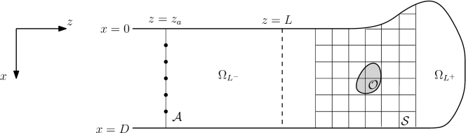
Figure 1: Schematic representation of the semi-infinite waveguide.

We also assume that the array measurements can be cast in the form of the so-called array response matrix, denoted by $\widehat{\Pi}$. This is an $N\times N$ complex matrix whose $(r,s)$ entry is the Fourier transform of the time traces of the echoes recorded at the $r$-th receiver when the $s$-th source emits a signal. In particular, we shall use the array response matrix for the scattered field that is due to the presence of an extended reflector $\mathcal{O}$ located somewhere in the bounded part of the waveguide delimited by the cross-section at $z=L$ (see Fig. 1). As usual, the scattered field is determined by subtracting the incident field from the total field.

Specifically, we consider a Cartesian coordinate system $(z,x)$, where $z$ denotes the main direction of propagation called hereafter range, and $x$ the cross-range direction taken to be positive downwards. Our terminating waveguide $\Omega$ consists of two subdomains: the semi-infinite strip $\Omega_{L^{-}}=(-\infty,L)\times(0,D)$ and a bounded domain in ${\mathbb{R}}^{2}$ denoted by $\Omega_{L^{+}}$. Let us also assume that all the inhomogeneities of the medium are contained in $\Omega_{L^{+}}$ while the medium is homogeneous in the semi-infinite strip $\Omega_{L^{-}}$, i.e. the wave speed may depend on range and cross-range in $\Omega_{L^{+}}$, and varies smoothly to the constant value that has for $z\leq L$. Note that the assumption of a constant wave speed in $\Omega_{L^{-}}$ may be relaxed by requiring the speed to depend on the cross-range variable $x$. However, to facilitate the presentation in this paper we will consistently assume that $\Omega_{L^{-}}$ is filled with a homogeneous medium.

The total field for our waveguide in the presence of a scatterer solves the scalar wave equation

(1) $$\Delta p^{\rm tot}(t,\mbox{$\vec{\bi{x}}$})-\frac{1}{c(\mbox{$\vec{\bi{x}}$})^{2}}\frac{\partial^{2}p^{\rm tot}(t,\mbox{$\vec{\bi{x}}$})}{\partial t^{2}}=-f(t,\mbox{$\vec{\bi{x}}$}),$$

where $\mbox{$\vec{\bi{x}}$}=(z,x)\in\Omega$ and the source term $f(t,\mbox{$\vec{\bi{x}}$})$ models a point-like source with time-harmonic dependence. Equation 1 is supplemented by homogeneous Dirichlet conditions on the boundary of $\Omega$. The scatterer is modeled as an acoustically hard scatterer with a homogeneous Neumann condition on $\partial\mathcal{O}$ and a suitable outgoing radiation condition is assumed as $z\rightarrow-\infty$. Moreover, we assume that the medium is quiet for $t\leq 0$, i.e. $p^{\rm tot}(t,\mbox{$\vec{\bi{x}}$})=0$ for $t\leq 0$. Note that the scalar wave equation that we consider here is used quite often instead of the full Maxwell’s or elastic wave equations since it captures the main features of the scattering problem.

By applying the Fourier transform

(2) $$\widehat{p}^{\rm tot}(\omega,\mbox{$\vec{\bi{x}}$})=\int\mathrm{e}^{i\omega t}p^{\rm tot}(t,\mbox{$\vec{\bi{x}}$})dt$$

on Eq. 1, we obtain the Helmholtz equation for the total field

(3) $$-\Delta\widehat{p}^{\rm tot}(\omega,\mbox{$\vec{\bi{x}}$})-k^{2}\eta(\mbox{$\vec{\bi{x}}$})\,\widehat{p}^{\rm tot}(\omega,\mbox{$\vec{\bi{x}}$})=\widehat{f}(\omega,\mbox{$\vec{\bi{x}}$}),\quad\mbox{$\vec{\bi{x}}$}\in\Omega,$$

where $\omega$ is the angular frequency, $k=\omega/c_{0}$ is the (real) wavenumber and $\eta(\mbox{$\vec{\bi{x}}$})=c^{2}_{0}/c^{2}(\mbox{$\vec{\bi{x}}$})$ is the index of refraction. (Notice that $\eta(\mbox{$\vec{\bi{x}}$})=1$ for all $\mbox{$\vec{\bi{x}}$}\in\Omega_{L^{-}}$.)

Let also $\mbox{$\widehat{G}$}(\mbox{$\vec{\bi{x}}$},\mbox{$\vec{\bi{x}}$}_{s};\omega)$ denote the Green’s function for the Helmholtz operator (and the associated boundary conditions) due to a point source located at $\mbox{$\vec{\bi{x}}$}_{s}=(z_{s},x_{s})\in\Omega$ and for a single frequency $\omega$, i.e. $\mbox{$\widehat{G}$}(\mbox{$\vec{\bi{x}}$},\mbox{$\vec{\bi{x}}$}_{s};\omega)$ is the solution of

(4) $$-\Delta\mbox{$\widehat{G}$}(\mbox{$\vec{\bi{x}}$},\mbox{$\vec{\bi{x}}$}_{s};\omega)-k^{2}\eta(\mbox{$\vec{\bi{x}}$})\mbox{$\widehat{G}$}(\mbox{$\vec{\bi{x}}$},\mbox{$\vec{\bi{x}}$}_{s};\omega)=\delta(\mbox{$\vec{\bi{x}}$}-\mbox{$\vec{\bi{x}}$}_{s}).$$

Finally, let $(\mu_{n},X_{n})$ be the eigenvalues and corresponding orthonormal eigenfunctions of the following vertical eigenvalue problem in the homogeneous part of the waveguide $\Omega_{L^{-}}$:

(5) $$X_{n}^{\prime\prime}(x)+\mu_{n}X(x)=0,\qquad X_{n}(0)=X_{n}(D)=0.$$

Henceforth we shall assume that there exists an index $M$ such that the constant value $k^{2}$ of the wavenumber satisfies in $\Omega_{L^{-}}$:

$$\lambda_{M}<k^{2}<\lambda_{M+1}.$$

In other words, $M$ is the number of propagating modes in $\Omega_{L}^{-}$. Let us also denote the horizontal wavenumbers in $\Omega_{L}^{-}$ by

(6) $$\beta_{n}=\left\{\begin{array}[]{ll}\sqrt{k^{2}-\mu_{n}},&1<n<M,\\ \mathrm{i}\sqrt{\mu_{n}-k^{2}},&n>M+1.\end{array}\right.$$

In what follows we will assume that the problems for the incident and the total fields, which are governed by the Helmholtz equation and satisfy the boundary conditions in the perturbed semi-infinite cylinder described before, are well-posed. Notice that for the incident field it is known, [Jones_1953], that the problem is well-posed except for a set of values of $k^{2}$ that are equal to point eigenvalues of the negative Laplacian associated with zero Dirichlet conditions on the boundary. This set is at most countable, it has no finite accumulation point and in many cases it is empty. For the total field there are examples in infinite waveguides that suggest existence of the so-called trapped modes, i.e. nonzero localized solutions of the associated homogeneous problem, see e.g. [EP_1998].

3 Imaging

Our main objective in this work is to form images of extended reflectors that lie somewhere in a terminating waveguide like the one described in the previous section. The usual steps that one may follow to this end, is to first identify a search domain $\mathcal{S}$ (see Fig. 1), discretize it using a grid, and then compute the value of an appropriate imaging functional in each grid point in $\mathcal{S}$. It is expected that these values, when they are graphically displayed in the search domain, should exhibit peaks that indicate the presence of the reflector.

3.1 Imaging with a full-aperture array

We shall first consider the easier case where the array spans the whole vertical cross-section of the waveguide. Moreover, although we are interested in imaging extended reflectors we will first examine the so-called passive imaging problem in order to motivate the use of the imaging functional that we will introduce next.

3.1.1 Passive Imaging

So, let us assume that a point source of unit strength, located at the point $\mbox{$\vec{\bi{x}}$}_{s}=(z_{s},x_{s})\in\Omega$, emits a signal that is recorded on a vertical array $\mathcal{A}$ located in $\Omega_{L^{-}}$. Moreover, we assume that the array $\mathcal{A}=\{\mbox{$\vec{\bi{x}}$}_{r}=(z_{a},x_{r})\}_{r=1}^{N}$, ($z_{a}<L$), spans the whole vertical cross-section of the waveguide as illustrated in Fig. 2. Our aim is to find the location of the source. In this case the array response matrix $\widehat{\Pi}$ at frequency $\omega$ reduces to a $N\times 1$ vector, whose $r$-th component equals the Green’s function evaluated at receiver $\mbox{$\vec{\bi{x}}$}_{r}$ due to the source $\mbox{$\vec{\bi{x}}$}_{s}$, i.e.

(7) $$\widehat{\Pi}(\mbox{$\vec{\bi{x}}$}_{r};\omega)=\mbox{$\widehat{G}$}(\mbox{$\vec{\bi{x}}$}_{r},\mbox{$\vec{\bi{x}}$}_{s};\omega).$$

In what follows we consider a monochromatic source and to simplify the notation we suppress parameter $\omega$ from the imaging functional and the Green’s function. The dependence on $\omega$ will be recalled in LABEL:sec:mf where imaging with multiple frequency data is considered.

Figure 2: Passive imaging setup in a terminated waveguide.

The imaging functional that we propose to use is based on the concept of phase conjugation, which may be physically interpreted by virtue of the Huygen’s principle. As pointed out in [JD_91], Huygen’s principle states that a propagating wave may be viewed as superposition of wavelets reemitted from a fictitious surface with amplitudes proportional to those of the original wave. In phase conjugation, which may be seen as the equivalent of time reversal in the frequency domain, the reemitted wavelets’ amplitudes are proportional to the complex conjugate of the corresponding ones in the original wave. These remarks lead naturally one to define the following classical phase conjugation imaging functional

(8) $$\mathcal{I}^{\scriptscriptstyle{\rm pc}}(\mbox{$\vec{\bi{y}}$}^{s})=\int_{\mathcal{A}}\overline{\mbox{$\widehat{G}$}(\mbox{$\vec{\bi{x}}$}_{r},\mbox{$\vec{\bi{x}}$}_{s})}\mbox{$\widehat{G}$}(\mbox{$\vec{\bi{y}}$}^{s},\mbox{$\vec{\bi{x}}$}_{r})dx,$$

where $\mbox{$\vec{\bi{x}}$}_{r}=(z_{a},x)\in\mathcal{A}$ and $\mbox{$\vec{\bi{y}}$}^{s}\in\mathcal{S}$. However, if we assume for a moment that apart from recording the value of the field on the array we would be able to record its normal derivative as well, then we may define the following imaging functional, which as we will show next has very nice theoretical properties. So let

(9) $$\mathcal{I}(\mbox{$\vec{\bi{y}}$}^{s}):=\int_{\mathcal{A}}\Big{(}\overline{\mbox{$\widehat{G}$}(\mbox{$\vec{\bi{x}}$}_{r},\mbox{$\vec{\bi{x}}$}_{s})}\nabla\mbox{$\widehat{G}$}(\mbox{$\vec{\bi{x}}$}_{r},\mbox{$\vec{\bi{y}}$}^{s})-\mbox{$\widehat{G}$}(\mbox{$\vec{\bi{x}}$}_{r},\mbox{$\vec{\bi{y}}$}^{s})\overline{\nabla\mbox{$\widehat{G}$}(\mbox{$\vec{\bi{x}}$}_{r},\mbox{$\vec{\bi{x}}$}_{s})}~{}\Big{)}\cdot\bi{\nu}\,dx,$$

where $\bi{\nu}$ is the outward-pointing unit normal vector to $\mathcal{A}$. Of course this functional is more complicated than phase conjugation but the following proposition shows that in order to compute $\mathcal{I}(\mbox{$\vec{\bi{y}}$}^{s})$ in a terminating waveguide it is required to know only the values of the wave field on the array and not its derivatives.

Proposition 3.1 (Kirchhoff-Helmholtz identity).

Assume that a point source is located in the terminating waveguide that we have described in Section 2 (see, also, Fig. 2), and that a vertical array $\mathcal{A}$, which spans the whole vertical cross-section of the waveguide, is located in $\Omega_{L^{-}}$. Then, the imaging functional that we have defined in (9) satisfies the following Kirchhoff-Helmholtz identity:

(10) $$\mathcal{I}(\mbox{$\vec{\bi{y}}$}^{s})=\mbox{$\widehat{G}$}(\mbox{$\vec{\bi{y}}$}^{s},\mbox{$\vec{\bi{x}}$}_{s})-\overline{\mbox{$\widehat{G}$}(\mbox{$\vec{\bi{y}}$}^{s},\mbox{$\vec{\bi{x}}$}_{s})}=2i{\rm Im}\,\mbox{$\widehat{G}$}(\mbox{$\vec{\bi{y}}^{\,\rm s}$},\mbox{$\vec{\bi{x}}$}_{s}).$$

Moreover, we can show that,

(11) $$\mathcal{I}(\mbox{$\vec{\bi{y}}$}^{s})=2i\sum_{n=1}^{M}\beta_{n}\,\overline{\mbox{$\widehat{G}$}_{n}(z_{a},\mbox{$\vec{\bi{x}}$}_{s})}\,\mbox{$\widehat{G}$}_{n}(z_{a},\mbox{$\vec{\bi{y}}$}^{s}),$$

where $\mbox{$\widehat{G}$}_{n}(z_{a},\cdot)$, $n=1,\ldots,M$, denote the first $M$ Fourier coefficients of the Green’s function (which correspond to the propagating modes) with respect to the orthonormal basis of $L^{2}(0,D)$ that is formed by the vertical eigenfunctions $X_{n}$, i.e.

(12) $$\mbox{$\widehat{G}$}_{n}(z_{a},\cdot)=\int_{0}^{D}\mbox{$\widehat{G}$}((z_{a},x^{\prime}),\cdot)\,X_{n}(x^{\prime})\,dx^{\prime}.$$

Proof. See LABEL:sec:KHpr.  $\Box$

The passive imaging functional

Motivated by Proposition 3.1 we define here our imaging functional for the passive case. Assuming that the array elements are dense enough, so that we may think of the array as being continuous, we define

(13) $$\widehat{\mathbb{Q}}_{n}=\int_{0}^{D}\widehat{\Pi}\big{(}\mbox{$\vec{\bi{x}}$}_{r};\omega\big{)}X_{n}(x)\,dx,\quad n=1\ldots,M,$$

to be the projection of the recorded field on the first $M$ eigenfunctions $X_{n}$, $n=1\ldots,M$, of the vertical eigenvalue problem Eq. 5. Notice that using Eq. 7, $\mathbb{Q}_{n}$ may be written as

$$\widehat{\mathbb{Q}}_{n} =\int_{0}^{D}\mbox{$\widehat{G}^{\scriptscriptstyle{R}}$}\big{(}(z_{a},x),\mbox{$\vec{\bi{x}}$}_{s}\big{)}X_{n}(x)\,dx=\mbox{$\widehat{G}_{n}^{\scriptscriptstyle{R}}$}(z_{a},\mbox{$\vec{\bi{x}}$}_{s}).$$

In view of Eq. 11 we define our imaging functional as:

(14) $$\mbox{$\mathcal{I}^{\scriptscriptstyle{\rm p}}$}(\mbox{$\vec{\bi{y}}$}^{s}):=\sum_{n=1}^{M}\beta_{n}\overline{\widehat{\mathbb{Q}}_{n}}\,\mbox{$\widehat{G}$}_{n}(z_{a},\mbox{$\vec{\bi{y}}$}^{s}).$$

Note that the evaluation of $\mbox{$\mathcal{I}^{\scriptscriptstyle{\rm p}}$}(\mbox{$\vec{\bi{y}}$}^{s})$, for $\mbox{$\vec{\bi{y}}$}^{s}\in\mathcal{S}$, requires only recordings of the wave field. Moreover, Eq. 10 and Eq. 11 ensure that

(15) $$\mbox{$\mathcal{I}^{\scriptscriptstyle{\rm p}}$}(\mbox{$\vec{\bi{y}}$}^{s})={\rm Im}\,\mbox{$\widehat{G}$}(\mbox{$\vec{\bi{y}}^{\,\rm s}$},\mbox{$\vec{\bi{x}}$}_{s}).$$

This last equation is a very interesting result, and says that the quality of the focusing in the image is determined by the imaginary part of the Green’s function in our waveguide. Therefore, a resolution analysis for $\mathcal{I}^{\scriptscriptstyle{\rm p}}$ will entail the study of the behaviour of ${\rm Im}\,\mbox{$\widehat{G}$}$.

Example 3.2 (Imaging a point source).

In order to provide to the reader a sense of how $\mbox{$\mathcal{I}^{\scriptscriptstyle{\rm p}}$}(\mbox{$\vec{\bi{y}}^{\,\rm s}$})$ behaves we consider the simple case of imaging a source in a homogeneous terminating waveguide that forms a semi-infinite strip, i.e. $\Omega=(-\infty,R)\times(0,D)$. We assume a reference wavenumber $k_{0}=\pi/10$ that corresponds to a reference wavelength $\lambda_{0}$, and take $D=10\lambda_{0}$ while the vertical (terminating) boundary is placed at $R=27.5\lambda_{0}$. In Fig. 3, we plot the modulus of equation Eq. 14, for a source placed at $\mbox{$\vec{\bi{x}}$}_{s}=(19,5)\lambda_{0}$ (shown in the plot as a white asterisk) and for a single frequency $f$ that corresponds to a wavenumber $k=0.973k_{0}$. This results to a number of propagating modes $M=19$. Finally our search domain is $\mathcal{S}=[11.5,26.5]\times[0,10]$, where all distances are expressed in terms of the reference wavelength $\lambda_{0}$.

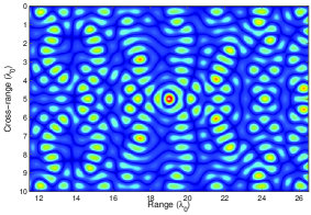
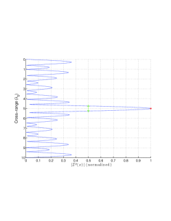
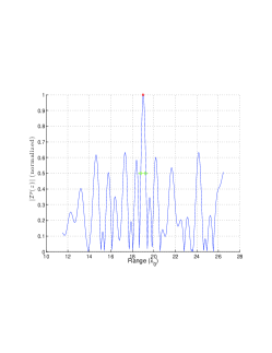
Figure 3: Normalized modulus of $\mathcal{I}^{\scriptscriptstyle{\rm p}}$ for a point source located at $\mbox{$\vec{\bi{x}}$}_{s}=(19,5)\,\lambda_{0}$ and for a single frequency corresponding to $k=0.973k_{0}$. Imaging on the whole search domain (left), for search points fixed at the correct range $z=z_{s}$ (middle) and at the correct cross-range $x=x_{s}$ (right). The green arrowed segment indicates length equal to $\lambda/2$ and a red asterisk points to the location of the source.

We observe that the $\mbox{$\mathcal{I}^{\scriptscriptstyle{\rm p}}$}(\mbox{$\vec{\bi{y}}^{\,\rm s}$})$ image, despite a relatively high noise level, displays a clear peak around $\mbox{$\vec{\bi{x}}$}_{s}$, which is a key property for an imaging functional.

3.1.2 Active Imaging

As a step forward to the general case of an extended scatterer, we will now deal with the active imaging problem where we are interested in locating a single point scatterer of unit reflectivity that is situated at $\mbox{$\vec{\bi{x}}$}^{\ast}=(z^{\ast},x^{\ast})$ while the array $\mathcal{A}$ is like the one in the passive imaging case as illustrated in Fig. 4.

Figure 4: Active imaging setup in a terminated waveguide.

Then, the $(s,r)$ entry of the array response matrix:

$$\widehat{\Pi}(\mbox{$\vec{\bi{x}}$}_{s},\mbox{$\vec{\bi{x}}$}_{r};\omega)=k^{2}\mbox{$\widehat{G}$}(\mbox{$\vec{\bi{x}}$}^{\ast},\mbox{$\vec{\bi{x}}$}_{s};\omega)\mbox{$\widehat{G}$}(\mbox{$\vec{\bi{x}}$}_{r},\mbox{$\vec{\bi{x}}$}^{\ast};\omega),$$

corresponds to the scattered signal received at $\mbox{$\vec{\bi{x}}$}_{r}$ when the point reflector at $x^{\ast}$ is illuminated by a unit amplitude signal emitted at frequency $\omega$ from a point source located at $\mbox{$\vec{\bi{x}}$}_{s}$. In what follows we suppress the multiplicative constant $k^{2}$, hence we assume that

(16) $$\widehat{\Pi}(\mbox{$\vec{\bi{x}}$}_{s},\mbox{$\vec{\bi{x}}$}_{r};\omega)=\mbox{$\widehat{G}$}(\mbox{$\vec{\bi{x}}$}^{\ast},\mbox{$\vec{\bi{x}}$}_{s};\omega)\mbox{$\widehat{G}$}(\mbox{$\vec{\bi{x}}$}_{r},\mbox{$\vec{\bi{x}}$}^{\ast};\omega).$$

In the mutiple-frequency case we can also remove this factor by rescaling the data matrix $\widehat{\Pi}(\mbox{$\vec{\bi{x}}$}_{s},\mbox{$\vec{\bi{x}}$}_{r};\omega)$ to be equal to $k^{-2}\widehat{\Pi}(\mbox{$\vec{\bi{x}}$}_{s},\mbox{$\vec{\bi{x}}$}_{r};\omega)$.

Assuming again that the array is continuous we define the projected response matrix $\widehat{\mathbb{Q}}$ as

(17) $$\widehat{\mathbb{Q}}_{nm}=\int_{0}^{D}\int_{0}^{D}\widehat{\Pi}(\mbox{$\vec{\bi{x}}$}_{s},\mbox{$\vec{\bi{x}}$}_{r};\omega)X_{n}(x_{s})X_{m}(x_{r})\,dx_{s}\,dx_{r},\quad n,m=1\ldots,M,$$

where $X_{n}$, $n=1\ldots,M$, are the first $M$ eigenfunctions of problem Eq. 5 as before.

The active imaging functional

A natural generalization of the imaging functional that we have proposed in the passive case is the following active imaging functional

(18) $$\mbox{$\mathcal{I}^{\scriptscriptstyle{\rm a}}$}(\mbox{$\vec{\bi{y}}^{\,\rm s}$}):=\sum_{n=1}^{M}\sum_{m=1}^{M}\beta_{n}\beta_{m}\overline{\widehat{\mathbb{Q}}_{nm}}\,\mbox{$\widehat{G}$}_{n}(z_{a},\mbox{$\vec{\bi{y}}^{\,\rm s}$})\,\mbox{$\widehat{G}$}_{m}(z_{a},\mbox{$\vec{\bi{y}}^{\,\rm s}$}),$$

defined for each point $\vec{\bi{y}}^{\,\rm s}$ in the search domain $S$.

Note that by replacing Eq. 16 into Eq. 17 and using the expression of $\mbox{$\widehat{G}$}_{n}$ given in Eq. 12, it is easy to show that

(19) $$\widehat{\mathbb{Q}}_{nm}=\mbox{$\widehat{G}$}_{n}(z_{a},\mbox{$\vec{\bi{x}}$}^{\ast})\,\mbox{$\widehat{G}$}_{m}(z_{a},\mbox{$\vec{\bi{x}}$}^{\ast}).$$

In turn, Eq. 18 now becomes,

$$\mbox{$\mathcal{I}^{\scriptscriptstyle{\rm a}}$}(\mbox{$\vec{\bi{y}}^{\,\rm s}$})=\sum_{n=1}^{M}\beta_{n}\,\overline{\mbox{$\widehat{G}$}_{n}(z_{a},\mbox{$\vec{\bi{x}}$}^{\ast})}\,\mbox{$\widehat{G}$}_{n}(z_{a},\mbox{$\vec{\bi{y}}^{\,\rm s}$})\sum_{m=1}^{M}\beta_{m}\,\overline{\mbox{$\widehat{G}$}_{m}(z_{a},\mbox{$\vec{\bi{x}}$}^{\ast})}\,\mbox{$\widehat{G}$}_{m}(z_{a},\mbox{$\vec{\bi{y}}^{\,\rm s}$}),$$

and Proposition 3.1 ensures that

(20) $$\mbox{$\mathcal{I}^{\scriptscriptstyle{\rm a}}$}(\mbox{$\vec{\bi{y}}^{\,\rm s}$})=\Big{(}{\rm Im}\,\mbox{$\widehat{G}$}(\mbox{$\vec{\bi{y}}^{\,\rm s}$},\mbox{$\vec{\bi{x}}$}^{\ast})\Big{)}^{2}.$$

Thus we deduce that the imaging functional Eq. 18 for a point scatterer behaves like the square of the imaginary part of the Green’s function.