Active Betweenness Cardinality: Algorithms and Applications

Abstract.

Centrality rankings such as degree, closeness, betweenness, Katz, PageRank, etc. are commonly used to identify critical nodes in a graph. These methods are based on two assumptions that restrict their wider applicability. First, they assume the exact topology of the network is available. Secondly, they do not take into account the activity over the network and only rely on its topology. However, in many applications, the network is autonomous, vast, and distributed, and it is hard to collect the exact topology. At the same time, the underlying pairwise activity between node pairs is not uniform and node criticality strongly depends on the activity on the underlying network.

In this paper, we propose active betweenness cardinality, as a new measure, where the node criticalities are based on not the static structure, but the activity of the network. We show how this metric can be computed efficiently by using only local information for a given node and how we can find the most critical nodes starting from only a few nodes. We also show how this metric can be used to monitor a network and identify failed nodes. We present experimental results to show effectiveness by demonstrating how the failed nodes can be identified by measuring active betweenness cardinality of a few nodes in the system.

1. Introduction

Identifying critical elements of a network has been at the heart of many efforts on infrastructure security and social network analysis. The critical elements are those, whose presence are essential for a network to maintain its functionality at or near its maximum. For an infrastructure network, a critical node may be a major hub, for an airline network, or a router in a communication network. In a social network, a critical element can be an influential person. Subsequently, the network science community have proposed many metrics to quantify the criticality of network elements and associated algorithms to compute these metrics efficiently.

A major thrust in this area has been network centrality, which assigns a number that is a measure for its importance to each node. The importance of a node varies from one application to another, and thus there have been many metrics to measure centrality. For instance, Closeness (Dekker, 2005) and harmonic centrality (Rochat, 2009) of a node are based on the distance from this node to all the other nodes. The smaller the distances are, the higher will be the centrality of the node. Betweenness centrality (Freeman, 1977) of a node on the other hand, is based on how often this node appears on a shortest path between any pair of nodes. The more often this node is on a shortest path, the higher will be its betweenness centrality. One can also consider degree centrality, which looks at the number of direct neighbors of a node, or its generalization, Katz centrality (Katz, 1953), which takes into account not only 1-hop neighbors as in degree centrality, but all 2, 3, … hop neighborhoods but decreases the contribution of each node based on the distance. For more detailed information of centrality measures, we refer the reader to (Sarıyüce et al., 2015). In this paper, we will work on a variant of betweenness centrality as we discuss below.

These measures provide a wide variety of valuable insight into graphs, but they all rely on two assumptions: (1) centrality of a node depends only on the topology of a graph and does not take into account the dynamics on the graph or how the graph is being utilized, and (2) we know the exact topology of the whole graph. These assumptions restrict the effectiveness and applicability of these methods. First, we cannot assume there will be an interaction between all pairs of nodes on a large graph at the same level or frequency. This may be due to lack of interest (e.g., not every user visits every page on the Web) or some nodes provide identical services and users only interact with the nearest such server (one goes to a close-by hospital, not necessarily all the hospitals). One question we could ask is that can we develop approaches with models that comprise probabilities of interactions between every pair of vertices? While this sounds good at first, building such a vast model with high confidence can be as burdensome as computing the centralities themselves. It should be noted that centrality measures were initiated by the social science studies on much smaller networks, where neither of the these two limitations apply. But one should be careful before applying the same ideas to current datasets, where the graphs are much larger and comprise nodes with identical functionalities.

The second problem is the assumption that we know the exact topology of the network. Many networks such as the Internet are vast, distributed, and autonomous. Moreover, both their topology and the dynamics on them keep evolving. Determining their exact topology or even predicting their topological features are far from trivial.

Here we propose a new approach for centrality that takes into account the network dynamics and does not require having access to the exact topology. We call our approach the Active Betweenness Cardinality (ABC) model. The metric for our model is the number of distinct pairs of nodes that communicate through this node within a specified period. Our data access model is that for any interaction through a node, we know the source and the destination. For a communication network, this would be the source IP and the destination IP; for an airline network, this would be departure and destination locations for each passenger. Note that, we can compute the ABC value of any node with only local computation on that node without knowing anything about the rest of the graph. As we will show in this paper, we can estimate this quantity efficiently (both in terms of runtime and memory) and accurately, using a sublinear algorithm. We will also show that we can search and identify nodes with high ABC values. Moreover, we will show that, the proposed metric can help us identify presence and location of changes in a network. We claim that this approach provides a critical capability for analysis for vast distributed networks.

Outline. The rest of the paper is organized as follows: Section 2 introduces the preliminaries on estimating set cardinalities and centrality on graphs. Section 3 presents our experimental setup. The proposed metric is explained in Section 4, followed by techniques that can approximate this metric and finding critical nodes starting from a small number of nodes. Section 5 presents how the proposed techniques can be used to detect significant changes in the network. Section 6 concludes the paper.

1.1. Our contributions:

This paper presents significant contributions on several fronts.

• A novel metric for criticality. We propose Active Betweenness Cardinality (ABC) metric to identify critical nodes in a network. This metric is based on the number of distinct pair of nodes that communicate through this node within a specified period.

• A sublinear algorithm to compute this metric. Proposed metric requires estimating the cardinality of a set, whose elements we observe with repetition. We use the hyperloglog algorithm to show that the proposed metric can be computed with a small amount of memory, making the proposed approach attractive for massive networks.

• Algorithms to find nodes that maximize this metric. Previous techniques can estimate the centrality of a node. Can we find nodes with the highest centrality values without exhaustive search? We designed an algorithm that finds high-centrality nodes by walking from a specified subset of nodes.

• Failure detection. We define critical elements as those nodes whose failure will affect the remainder of the system. Symmetrically, these elements are affected by failure of other important components in the system. We show that out metric can be used to identify presence and location of failures of other network elements.

• Thorough experimental analysis. We show that the effectiveness of all methods through detailed empirical studies. We show that the proposed metric can be estimated efficiently using only local algorithms and show how this algorithms can be used to search for the most critical nodes. We also show that the new metric can be used to detect failed nodes by suing classification methods.

2. Preliminaries

Let $G=(V,E)$ be a simple undirected, unweighted graph where $n$ is the number of nodes and $m$ is the number of edges. We assume that any pair of nodes can interact with each other by sending/receiving some information and any interaction can be repeated. We define $G$ as an active network. If there is an interaction between nodes $u$ and $v$, it happens via a path $p$ between $u$ and $v$, and all the communication thereafter also happens via the same path $p$. For consistency with the real-world routing algorithms (Malkin, 1998), we restrict $p$ to be one of the shortest paths between $u$ and $v$. We define the number of unique interactions that are transmitted by a node $u$ as the cardinality of $u$, denoted as $\rho(u)$. We want to detect the nodes with large cardinality by using only the local information.

2.1. Cardinality Estimation on Data Streams

An important part of our problem is about estimating the cardinality of a data stream, which is also called the count-distinct problem. We observe the elements of a set in a stream which can occur repeatedly, not just once. Our goal is to estimate the cardinality of this set.

Formally, given a stream $x_{0},x_{1},x_{2},\ldots x_{K}$ with repetitions, where $x_{i}\in S$ for $i=0,\ldots K$. Note that due to repetitions $x_{i}$ and $x_{j}$ are not necessarily distinct. We have a dual objective function: we want to estimate $|S|$, the cardinality of the set $S$, as accurately as possible by using minimal storage. For the purposes of this paper, the elements of the stream will be the interacting pairs, and each entry in the system will be one message exchange.

The difficulty of this problem lies in handling the repetitions. A trivial solution is to maintain a hash table to keep track of the previously observed elements. This can give an exact solution, but associated memory requirement will be linear in the size of the set $S$, which is impractical for many real- world scenarios. The algorithmic challenge is in drastically reducing storage, while maintaining accuracy. Randomized algorithms are helpful to address this challenge. Using randomization for the cardinality estimation was initiated by Flajolet and Martin (Flajolet and Martin, 1985). Since then, it has been the subject of many research efforts. A thorough survey of this literature is beyond the scope of this paper and we refer to readers to (Heule et al., 2013) and references therein. Our methods do not depend on a particular cardinality estimation method, but we briefly describe the algorithms used in our experiments to show that cardinalities on data streams can be estimated accurately and efficiently.

The Hyperloglog (HLL) algorithm for cardinality estimation was proposed by Flajolet et al. (Flajolet et al., 2007) as an improvement over the Loglog algorithm (Durand and Flajolet, 2003), and it is the best algorithm, both in theory and in practice, for estimating large cardinalities (Heule et al., 2013). Hyperloglog algorithm is based on a hash function that can transform stream elements into uniformly distributed random numbers. The key observation is that the cardinality of a multiset of uniformly distributed random numbers can be estimated by the maximum number of leading zeros in their binary representations – if the maximum number of leading zeros observed is $n$, then the cardinality of the set can be estimated as $2^{n}$. However, a direct application of this idea suffers from a large variance. To solve this, the input is divided into $m=2^{p}$ separate buckets based on the leading $p$ bits of each number to estimate the cardinality of each bucket and then these individual estimates are combined using harmonic mean to get an estimate for the full set. As a practical guide on the performance, the Hyperloglog algorithm can compute estimates with relative error of $1.04/\sqrt{m}$ and requires $O(\epsilon^{-2}\log\log n+\log n)$ space to provide an $(1\pm\epsilon)$ -approximation with a high probability of success. In our experiments we used the Hyperloglog method with parameter $p=12$ bits, and thus, $m=2^{p}=2^{12}$ buckets.

2.2. Centrality Measures

The centrality metrics play an important role in network and graph analysis since they are related with several concepts such as reachability, importance, influence, and power (Şimşek and Barto, 2009; Jin et al., 2010; Merrer and Trédan, 2009; Pham and Klamma, 2010; Shi and Zhang, 2011). Betweenness and closeness centralities (BC and CC) are two such metrics. However, the complexity of the best algorithms to compute them are unbearable for today’s large-scale networks: it is $\mathcal{O}(nm)$ for unweighted networks (Brandes, 2001). This already makes the problem hard even for medium-scale graphs, and thus many research efforts have focused on efficiently utilizing state of the art HPC platforms for this problem (Jia et al., 2011; Sarıyüce et al., 2013, 2015; Shi and Zhang, 2011; Pande and Bader, 2011).

Let $G=(V,E)$ be a connected graph. Let $\sigma_{st}$ be the number of shortest paths from a source $s\in V$ to a target $t\in V$, and $\sigma_{st}(v)$ be the number of such $s$-$t$ paths passing through a node $v\in V$, $v\neq s,t$. Let $\delta_{st}(v)=\frac{\sigma_{st}(v)}{\sigma_{st}}$, the fraction of the shortest $s$-$t$ paths passing through $v$ among all shortest $s$-$t$ paths. The betweenness centrality of $v$ is defined by

(1) $$BC(v)=\sum_{s\neq v\neq t\in V}\delta_{st}(v).$$

Brandes proposed an algorithm to compute $BC(v)$ for all $v\in V$ that is based on the accumulation of pair dependencies over target nodes (Brandes, 2001), which has $O(mn)$ complexity. Scaling the betweenness centrality computation to large networks is impractical. To alleviate this problem, approximation schemes (Bader et al., 2007; Riondato and Kornaropoulos, 2014; Riondato and Upfal, 2016) and parallel algorithms (Madduri et al., 2009; Cohen, 2015; Sarıyüce et al., 2015) are developed.

Several works have been proposed to estimate such centrality measures using sublinear memory in the size of the graph (Boldi and Vigna, 2013; Priest and Cybenko, 2017). Priest and Cybenko (Priest and Cybenko, 2017) propose an algorithm that makes use of CountSketch (Charikar et al., 2002) algorithm. HyperBall  (Boldi and Vigna, 2013) work utilizes HyperLogLog variants to approximate centralities that depends on the nodes within a certain ball radius $r$, such as Lin’s centrality, Harmonic centrality and Closeness centrality.

However, all of those approaches focus on the network topology information to infer the centrality, i.e., communications between each pair of nodes are assumed to be same and non-repetitive, and need the global graph information to highlight the most central nodes.

In our work, we propose local algorithms that can find the most critical nodes. Our focus is on active networks where there can be non-uniform and repetitive communications between nodes, which is not studied before to the best of our knowledge.

3. Experimental Setup

3.1. Graph Instances

Table 1. Graphs used in the experiments

Graph	#Nodes	#Edges	Degree
			min	avg	max
World Airports	2,939	30,501	1	10.37	237
AS-733	6,474	12,572	1	3.88	1,458
Oregon-01	10,670	22,002	0	4.12	2,312

We will present results on three networks that represent infrastructure topologies. Properties of these three networks: Airport (Opsahl et al., 2010), AS-733 (Leskovec and Krevl, 2014) and Oregon-01 (Leskovec and Krevl, 2014) are presented in Table 1. AS-733 and Oregon-01 are the graphs of autonomous systems (AS), inferred from Oregon route- views on 1/2/2000 and 3/31/2001, respectively. In these networks, nodes correspond to routers and the edges correspond to connections between these routers. In our model, ABC of a router will be the number of distinct IP pairs that communicate through that router. Thus this will be the number of communicating pairs that will be affected if the router were to fail. Alternatively, one can look at the number of distinct IPs (source or destination), using the same algorithmic framework, but communicating pairs provide a better handle on the topological changes as we will describe later.

In the Airports graph, nodes correspond to airports and there is an edge between two nodes if there is a flight between the two corresponding airports. In this case, our metric corresponds to how many departure/destination pairs go through a given airport.

3.2. Modeling Network Activity

Modeling the activities on a network is a complicated problem and a challenge in itself. For this paper, our goal is to generate instances to empirically test our proposed methods. Below, we first describe our data sets and then how we generated the activity on these networks.

3.2.1. Communication Pathways

We assume communication between a pair of nodes follows a shortest path and the underlying graph is connected. In our experiments, we pick a random shortest path among all shortest paths for each source and destination pair as their communication path, store this information, and use the same path throughout the experiment. In practice, communication between a pair of nodes does not necessarily follow the shortest path, but a short path. Airlines design their flights as such for efficiency and fewer hubs usually mean cheaper flights, and people prefer to take shorter flights. In communication networks, each router in a network passes the incoming packets to a specific neighbor router according to its routing table, where it stores the next-hop neighbor information (the neighbor it should pass the packet to) based on the prefix of the destination address. These tables are usually set for better communication quality, which aligns well with shorter paths. Unless there is a change in the graph structure; such as, a disconnection from or a new node connection to the network, the communication paths are unaffected. When there is a change in the graph structure, the shortest paths for the affected nodes are recomputed.

We want to note that main contributions of this paper are independent of the particular routing method used in the underlying system. Our shortest path approximation can be replaced with any other path finding algorithm. Such changes may affect the specific numbers per network and nodes, but the performances of the algorithms will be invariant.

3.2.2. Modeling the Node Activities

How often does a pair of nodes communicate? We need a model that answers this question for our experiments. In our experiments, we used a model that assigns a send frequency level and a receive frequency level to each node in the graph, and the probability of a communication from node $u$ to node $v$ is proportional to the product of send frequency level of node $u$ to the receive frequency level of node $v$. This is inspired by the Chung-Lu model (Chung and Lu, 2002) and its generalization for directed graph topologies (Meyers et al., 2006), where vertices are assigned in and out degrees (analogous to active frequencies in our case), and the probability of an edge is proportional to the product of the in-degree of one vertex and the out- degree of the other vertex.

We have tested our approach with uniform random distribution, Gaussian (normal), and power-law distribution. Our experiments showed that although the actual node rankings depend on the selected distribution, the algorithm and how it works is not dependent on it. In the rest of this paper, we present the results using the Gaussian distribution since it is widely used to represent and model real-life distributions in many domains.

3.2.3. Time Window of Activities

The measures proposed in this paper are time dependent. The number of pairs that communicate through a node will increase in time, but converges to the maximum number of pairs that communicate through it. In our experiments, we have used a sufficiently long time frame to observe the numbers of convergence to avoid additional variances due to our node activity levels. For practical purposes, we define interval as the number of communications over the graph.

4. Active Betweenness Cardinality

We will start this section with introducing our new proposed metric to measure node importance that takes the network activity levels into account and does not require full access to the graph. Next, we show how this quantity can be estimated efficiently using the Hyperloglog algorithm on a given node. Given the ability to accurately estimate this quantity on a given node, the next step is to find those nodes for which this quantity is the highest. Note that we can find such nodes by applying the same estimation technique to all nodes of the graph. However, that assumes we know and have direct access to all the nodes in the graph, which is one of the two basic premises of this work. Moreover, we are interested in analyzing massive, distributed systems like the Internet. As such, running a process on each router in such a system is different than making a pass over all nodes of a graph that resides in memory.

4.1. A New Metric for Node Criticality on Active Networks

In this section we introduce Active Betweenness Cardinality (ABC) as a new metric that measures node criticality not only based on topology, but on the activity level of the network. The proposed method also has algorithmic advantage that it can be computed based on only local information and we do not need to know the exact topology of the network.

Finding critical nodes in a graph has been studied in depth in the literature, with centrality based measures being a major thrust. Our proposed metric, inspired by the centrality ideas, betweenness centrality in particular, but it differs from these approaches in two major ways. Present methods for centrality rely on two assumptions: (1) centrality of a node depends only on the topology of a graph and do not take into account the dynamics on the graph or how the graph is being utilized, and (2) we know the exact topology of the whole graph.

These assumptions restrict the effectiveness and applicability of these methods. First, we cannot assume there will be an interaction between all pair of nodes on a large graph at the same level or frequency. This may be due to lack of interest (e.g., not every user visits every page on the Web) or some nodes provide identical services and users only interact with the nearest such server (one goes to a close-by hospital, not necessarily all the hospitals). One question we could ask is can we develop approaches with models that comprise probabilities of interactions between every pair of vertices? While this sounds good at first, building such a vast model with high confidence can be as burdensome as computing the centralities themselves. It should be noted that centrality measures were initiated by the social science studies on much smaller networks, where neither of the two limitations above apply. But one should be careful before applying the same ideas to current datasets, where the graphs are much larger and comprise nodes with identical functionalities.

The second problem is the assumption that we know the exact topology of the network. Many networks such as the Internet are vast, distributed, and autonomous. Moreover, both their topology and the dynamics on them keep evolving. Determining their exact topology or even predicting their topological features is far from trivial.

Here we propose a new metric, active betweenness cardinality, that avoids both problems.

Definition 4.1.

Active Betweenness Cardinality (ABC) of node $v$ for time, period $[t_{s},t_{f}]$, $ABC(v,t_{s},t_{f})$ is the number of distinct $\langle s,d,f\rangle$ tuples for a go-through node $v$, where $s$ and $d$ are the source and destination nodes of the communication, which we will also call as transaction, and $f$ represents the features associated with the transaction.

Note that, this metric is time dependent. However, as the difference between the start and end times increase, the metric converges. In our experiments, we have used the estimate after conversion, and will not specify the time intervals in the remainder of the paper. The features $f$, can be used to focus the analysis on certain types of activities in the network. For instance, we can only investigate trucks, not all vehicles, or we can focus only on http traffic in a network. In our experiments we have used any specific features. We will only refer to the ABC value of a vertex, when the time interval is clear from the context.

4.2. Computing ABC Accurately and Efficiently

In this section, we will show how the ABC metric can be computed efficiently, using only local information. Computing the ABC of a node corresponds to the count-distinct problem, which we have presented earlier in Section 2.1. We are interested in handling massive graphs with heavy traffic, which prohibits exact calculations due to speed of data arrival and memory requirements. Instead, we will use provably accurate approximation algorithms, specifically the HyperLogLog (HLL) algorithm, which was also discussed in Section 2.1. We will start with verifying that this techniques provides accurate estimations, as this technique will be the building block for other techniques in the remainder of the paper. Note that this technique does not require any information about the remainder of the network. All we need to know is the source and destination of each transaction that go through the node.

The results of our experiments are presented in Figure 1. In this figure each data point corresponds to the ABC of a different vertex in the World Airports Graph for one interval of size 50,000 transactions. The x-axis corresponds to the exact cardinality computed using the set approach, while the y-axis corresponds the approximation provided by the HLL algorithms. The red line corresponds to the ideal solution such that $x=y$, and the two green lines correspond to 2% over and under approximation, i.e., y=1.02x and y=0.98x.

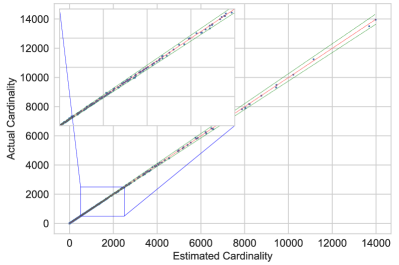
Figure 1. The actual unique number of (src,dest) pairs for each node vs HyperLogLog estimates. The red line is $y=x$ and green ones are $\pm 2\%$ error ranges.

As can be seen in Figure 1, the hyperloglog estimator consistently provides good estimates. always within 2%. We have run these experiments 20 times with different random seeds to generate different instances. Average Pearson Correlation Coefficient for Actual and HLL estimated cardinalities was 0.99994. The accuracy of HLL estimates is well-studied, thus we will not be presenting any further experiments here. But we hope that this experiment helps those who are not familiar with HLL techniques and show that the HLL algorithms works well in this case as well.

4.3. Finding Nodes with Highest ABC Scores

The results of the previous section show that we can efficiently estimate the ABC value of a given node. But how do we find the nodes with highest scores when we do not even know about the presence of nodes in the rest of the graph. If we knew and had access to all the nodes in the graph, we could have computed the estimates on all nodes to identify the most critical nodes (those with highest ABC scores). However, this is not feasible in a vast and autonomous system like the Internet. Here, we propose a set of heuristic algorithms that searches for the nodes with highest ABC scores, in a distributed fashion, starting from a handful of nodes. Below, we will describe our search strategies and experimentally show their effectiveness.

4.3.1. Search Strategies

Our techniques are based on choosing one of the neighbors of the current node that is most promising to have a higher ABC score than the current node and repeat. In all cases, we avoid backtracking to the node, where we came from. Starting from $C$ seed nodes, all of the search strategies iteratively selects next $C$ nodes to continue to search. We call each iteration a hop.

We show a number of approaches to traverse the graph and find important nodes: (i) traverse toward the neighbor with highest cardinality (via the edge ABC value), (ii) biased random walk to one of the neighbors where random walk probability of each neighbor is proportional to the cardinality of the edge between these two nodes, (iii) coordinating among multiple searches to investigate best overall alternatives.

Jump to Best Neighbor (BN): For each neighbor of the current node, or in another words, for each edge of the current node, we maintain an HLL estimator that counts the distinct pairs that communicated through that neighbor/edge. Intuitively, if we have an important neighbor, it would acquire most of our communication output. Alternatively, the current node is the important neighbor of that node that provides most of its input. Following that intuition, we select the out-neighbor that has the highest cardinality on the edge that connects the current node to that node as the candidate. We also propose a variation of BN that excludes selecting the nodes with only one out-neighbor, and we call that BN-1x.

Jump with Random Walk (RW): Jumping to the highest neighbor could get us stuck at a local extrema where we do not have anywhere else to jump since we do not allow jumping back to a previously observed node. For this purpose, we implemented a Random Walk-like approach where the neighbors have probabilities proportional to their corresponding HLL estimators on the edges. For example, let us consider a node A with out-neighbors X, Y, W, and Z. The HLL estimations on the edges are {60, 32, 80, 28} respectively. With BN strategy, we would jump to W and we might miss the chance to see X. We normalize these values and get {0.3, 0.4, 0.16, 0.14}. Then, we randomly pick one of the neighbors with this probability distribution as the candidate. Similar to BN, propose a variation of RW that excludes selecting the nodes with only one out-neighbor, and we call that RW-1x.

Biggest Collective Neighbor Selection (BCN): An alternative approach is instead of each node selecting one node to jump-to, collectively they can decide which nodes should be next subset of nodes to evaluate. This will speed up the convergence in cases where one of the subset nodes have all important neighbors but all the others are not necessarily as important. For example, consider a scenario that the set of nodes we are evaluating are {A, B, C, D }, and all the neighbors of node A has cardinalities in the scale of ten thousands and the neighbors of B, C, and D, have cardinalities in the scale of thousands. In such a case, it would make much more sense to select the nodes of new subset all from the neighbors of node A instead of picking one neighbor from each node. Converting this to a more general form, we select the top $C$ non-observed neighbors of all neighbors of current subset.

4.3.2. Quality Metric for Search Strategies

In this section we define the quality metrics for the presented strategies to find critical nodes. First metric is one-to-one correspondence of the critical nodes found and the ground truth. Second, the total (sum of) cardinality value found compared to the ground truth. Since what constitutes a ground truth depends on the active communication and activity of nodes, we need to decide what is ground truth for that specific configuration and settings. Hence, we generate a baseline from 400 runs with the same flow probability distributions, then average the ABC scores of each node to get a baseline for our experiments.

Top-$K$ Found Matches: For all algorithms, we compare the top $K$ nodes found with the top $K$ in the baseline. If the node found by the algorithm is among the top $K$ in the baseline, then we count this as a hit (success). So, perfect result would be to find $K$ out of $K$. We have run the experiment sets for 20 times and averaged the results.

Total Cardinality of Top-$K$ Found: If the cardinalities of the most critical nodes are not distinguishably different, comparing top-$K$ vertices against ground truth will not be fair. For such cases we simply compare the the sum of the total cardinality of top-$K$ found against the sum of the total cardinality of top-$K$ in baseline.

4.3.3. Experimental Results

Figure 2 shows the comparison of the search strategies for the three test graphs we have. The first two strategies are the random walk selections RW and RW-1x, second two are the best neighbor selections, BN and BN-1x, and the last one is the collective best neighbor selection strategy, BCN. Figure 2(a) shows all five alternatives for AS Graph. Figure 2(b) and 2(c) presents only the BN-1x and BCN to show the trend of the algorithms do not change much when different graphs are in question. Each bar represents the number of nodes in the search set, i.e., $C=\{4,8,12,16,20\}$.

As seen in Figure 2, as expected, as the search set size, $C$, gets bigger, so the quality of the result. However, even with modest sizes of $C$, where $C\approxeq K$, we can identify a large portion of the critical nodes. In addition, our search strategies requires small number of hops to stabilize, and they succeed to identify large portion of the critical nodes with RW and BN variants, and all top-$K$ with BCN. The figure also depicts that the quality of the approaches increase from top to bottom, having BCN the best and BN-1x the second best while random walk approaches have slightly worse results. Moreover, it shows that the results tend to converge in less than 7 hops for all 3 of the graphs. Finally, BCN also converges much quickly than the other variants. One could argue that the BCN strategy requires a collective selection, thus, more difficult deploy as a distributed strategy. We show the results of BN-1x together with BCN for all 3 graphs for this strategy to show one can use BN-1x instead of BCN and still have similarly high-quality result.

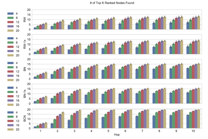
(a) AS Graph (Top to bottom: RW, RW-1x, BN, BN-1x, BCN)

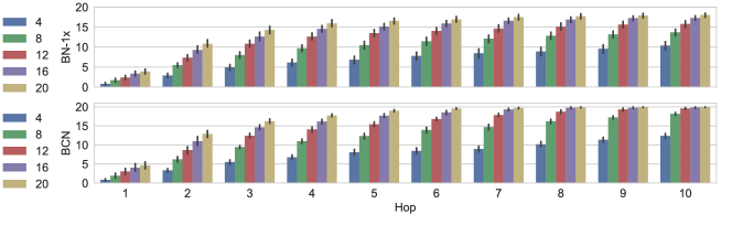
(b) World Airports Graph (BCN)

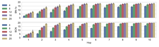
(c) Oregon Graph (BCN)

Figure 2. Top-$K$ found matches for five search strategies.

Figure 3 shows a comparison of the search strategies using our second metric, total cardinality of top-$K$ found, which is displayed as blue solid line on the chart. As in Figure 2, we displayed all five search strategies for AS graph, and strategies BN-1x and BCN for the other two graphs. The total cardinality found by each algorithm gets very close to the one identified in baseline, telling us top critical nodes have very similar cardinalities, thus those the BN and RW algorithms missed in Figure 2 from top-$K$ may not be much more critical than what those nodes found in terms of the nodes that depend on them. Similar to previous experiment, if fully distributed algorithm is preferred, one can use BN-1x instead of BCN and still have high-quality result.

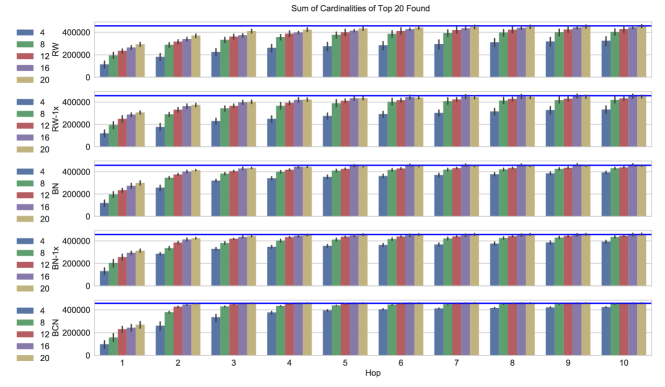
(a) AS Graph (Top to bottom: RW, RW-1x, BN, BN-1x, BCN)

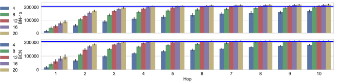
(b) World Airports Graph (BN-1x, BCN)

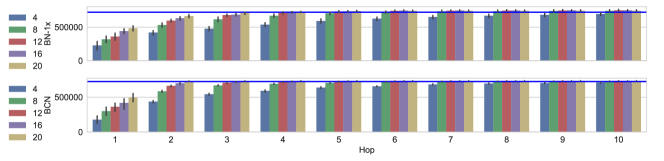
(c) Oregon Graph (BN-1x, BCN)

Figure 3. Total Cardinality of Top-$K$ Found for five search strategies.

5. Detecting Changes in Network

In this section, we showcase how the ABC values can be used to monitor a network and detect significant changes in the network topology. We first show how to detect the failure of a critical node by using a small number of sensors, then we discuss how to locate those nodes. We restrict ourselves to detecting failures of nodes with high ABC scores (e.g., top 200 or 400), as failures of such nodes make an overall impact on the functionality of the network. The question is if this change can be captured by our metrics by using a limited number of sensors. Failure of nodes with low ABC scores on the other hand is much harder to detect, as their absence is not expected to make an overall impact, and require sensors that are very close.

The critical observation for our methods is that the ABC values provide a stable baseline with very small variance, when the underlying network is stable. However, the same ABC scores are sensitive to the changes in the network, as we will show later. Here we first want to present the stable, low-variance nature of ABC scores in the network. Figure 4 shows the top 50 ABC values of the Airports graph for an interval size of 200,000. Experiments are repeated 400 times with the same communication probability distribution. In this figure, the box corresponds to the first and third quartiles. Whiskers show the range for $\pm 1.5\times IQR$, where $IQR$ is the difference between the third and first quantile values. Any outliers would have been marked with plus signs, but as can be seen there are no outliers, and the variances are extremely small, forming a good baseline to detect any changes.

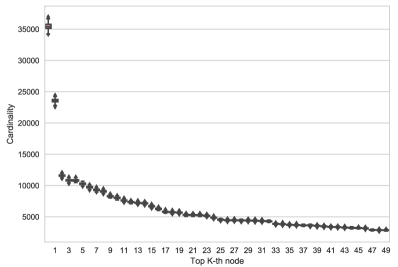
Figure 4. The ranges of Top 50 ABC values for the Airports graph for 200,000 transactions after 400 experiments with the same communication probability distribution. The box corresponds to the first and third quartiles. Whiskers show the range for $\pm 1.5\times IQR$, where $IQR$ is the difference between the third and first quantile values. Any outliers would have been marked with plus signs.

5.1. Detecting the Removal of Critical Nodes

We first discuss our approach to characterize what is normal and how we predict an anomaly based on only positive samples.

5.1.1. Characterizing Normal

One way to detect anomalies is to generate many examples that describe the system at its normal state and use them to build a distribution to define the normal. In our experiments we generate 200 examples and describe the state of the system as a 20 dimensional vector, which are the ABC values of critical nodes chosen randomly out of the top 200 nodes. We have used these examples to train OneClassSVM(Pedregosa et al., 2011) to form a model, and for each test case, it checks whether the description fits into normal or anomalous. We generated test cases by removing (10, 20, 30, or 50 nodes) out of the top 200 nodes.

Overall, we observed 80% accuracy. Such an accuracy is high for an approach where only positive examples are provided. However, test cases comprised significant failures that involve with many failed nodes. We observed that affects of failures remain local, even when significant. Failure of one node may double the ABC value of another node, which is sufficient. However, this effect can be minimal within the full-scale system, as it is absorbed locally. This motivated us to use supervised approaches which we explain next.

5.1.2. Binary Classification with failure examples

We train the algorithm with both the baseline and a set of results for anomaly cases where we also provide a label for each case, i.e. $0$ for normal, and $1$ for anomaly. Anomalies were based on removal of (10, 20, 30, or 50 nodes) out of the top 200 nodes. We have experimented with classification algorithms SVM (with linear and Gaussian (rbf) kernels), Linear Regression, Decision Trees, ExtraTrees, AdaBoost, Neural Networks (L-BFGS, Adam) and Ensemble (Weighted Voting based) of these in the python library scikit-learn(Pedregosa et al., 2011). We have found SVM with Gaussian kernel to be effective and fast.

We do 10-fold cross validation (Pedregosa et al., 2011). In our experiments we have seen the supervised learning have near $100\%$ accuracy in sensing the removal of a critical node subset. With this success, we investigated whether we can detect the location of the failure, not only the presence of the failure.

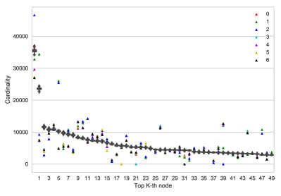
Figure 5. Box and Whiskers range for regular case and 7 instances of removal of critical nodes. The box corresponds to the first and third quartiles. Whiskers show the range for $\pm 1.5\times IQR$, where $IQR$ is the difference between the third and first quantile values.

5.2. Locating the Failure

Now that we can detect the presence of a failure, can we go a sep further and detect which node failed? The results in Figure 5 motivate our work. In this figure, we show how the top 50 ABC values change after failure of the top 6 nodes. In this figure label 0, corresponds to no failures, and the labels 1-6 correspond to failure of the node with the corresponding ABC rank. We plot these results on the baseline of Figure 4. As the figure shows, each failure pushes at least one ABC value significantly out of range. The question is whether we can identify a combination that can help us uniquely identify each failure.

The problem would be trivial, if we have sensor on each of the top K nodes. But we want to be able to infer beyond what we can observe directly. So instead we use the nodes ranked from $10{th}$ to $30{th}$ to predict failures of top 7 nodes. We assume single failures and only one important node from top 7 nodes is removed at one time. We train our classification algorithm with the baseline and a sample set of 200 instances for the removal of each of top 7 nodes. We test our algorithm with 10-fold cross validation (Pedregosa et al., 2011).

Figures 6 and 7 show the confusion matrices for 8 labels (Zero is when there is no change in the graph, i = 1 through 7 is the removal of top $i-{th}$ node) for 9 different classification algorithms we experimented with (namely, Linear SVC (Support Vector Machines with Linear Kernel), RBFSVC (Support Vector Machines with RBF (radial basis function, Gaussian) Kernel), Decision Trees, Extra Trees, Logistic Regression, AdaBoost, Artificial Neural Networks L-BFGS (Limited Memory Broyden-Fletcher-Goldfarb-Shanno) algorithm, Artificial Neural Networks (Adam method), and lastly the weighted Voting Ensemble). We used the implementations of these algorithms in the python library scikit-learn(Pedregosa et al., 2011).

These confusion matrices show the count of real and predicted label count for each instance in the test set. Having a diagonal matrix (where all entries outside the main diagonal are zero) is the perfect classification where the algorithm manages to successfully predict the actual label of each test case. Thus, Figures 6 and 7 show that the SVM Classifier with RBF kernel gives the best results. (Although some other algorithms also give the same amount of correct answers in this experiment, we have seen that RBFSVC works fast and better overall including the other sensing/detecting experiments.)

Overall, the results show that the ABC values can help accurately identify a missing node among the top nodes. It is worth noting that a naïve guessing approach would have ${\sim}15\%$ accuracy with a balanced training set.

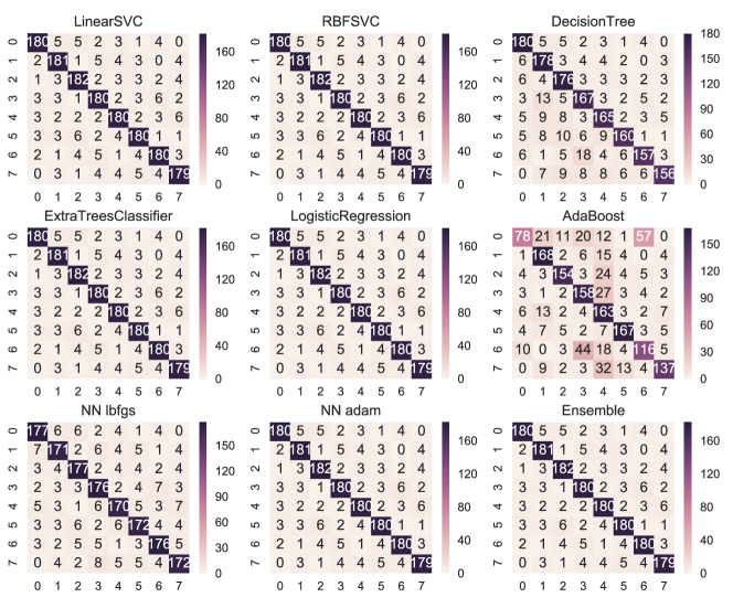
Figure 6. AS-733 Graph; Comparison of classification approaches. Detecting which one of top K nodes is disconnected using the top M nodes. ( k = 7, m= 40 in this case).

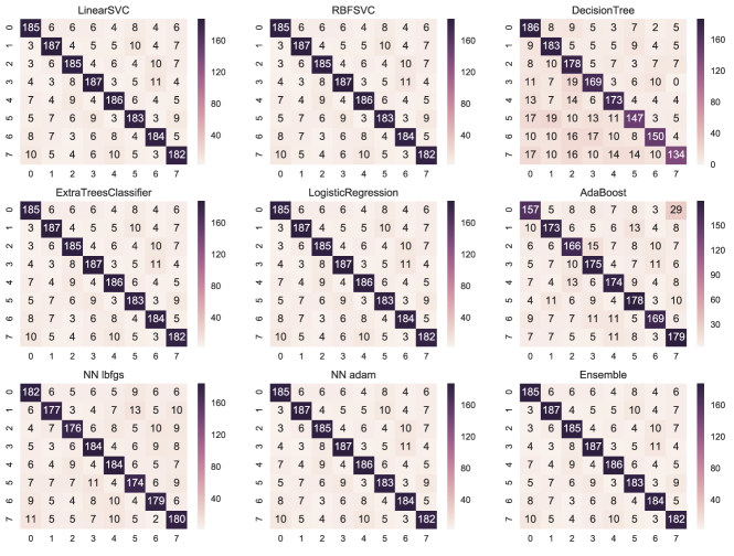
Figure 7. Airports Graph; Comparison of Machine Learning Approaches. Detecting which one of top K nodes is disconnected using the top M nodes. ( k = 7, m= 40 in this case).

5.2.1. Minimizing the Number of Sensors

If we can detect changes in top $7$ nodes using top $20$ nodes excluding top 7, then the next question to ask is, ”What is the minimum number of nodes to be observed to detect changes in the top $K$ nodes?” For this, we disconnect top $K$ nodes one by one and try to detect the changes using the remaining top $M-1$ nodes’ ABC values. Then, create a matrix to present which ones can classify the changes caused by which other nodes. Later, this matrix can be used to find the minimum required number of nodes to be observed to detect changes on all top K nodes.

To see what is the minimum we need, we tested how much we can identify using only one feature to train our machine learning algorithm. We use one of the top 20 nodes one by one as feature and train the algorithm with the baseline set of 200 and a set of 200 instances for the removal of top 7 nodes one by one. Assuming there is no other change in the graph, we store the accuracy achieved by each feature for each label in a feature - label matrix. Figure 8 show this matrix. According to the tolerance the context has, one may say that a $75\%$ accuracy may be enough, or may want at least $90\%$ accuracy.

The next step to further utilize this information would be to find the minimal number of elements required to successfully detect changes in any of these top $K$ nodes under the assumption that we do not have any concurrent node failures. This question is also known as minimum set cover problem in other domains, where we are trying to cover all the columns with the minimal number of rows selected. For example, in Figure 8 we can select $3{rd}$ and $5{th}$ as our features to successfully cover all the columns (labels/classes). In Figure 9, we can select $10{th}$ feature alone to have $75\%$ accuracy for first and last labels, and above $96\%$ for the others. Or, we can select $10{th}$ and $11{th}$ together to cover all of them with above $96\%$ accuracy.

We also repeated this experiment using not only one but combination of 2 and 3 nodes as the feature set to confirm that using the nodes together would work and highly probably increase the accuracy compared to using only one feature. Due a to space limitations, the visual results are not presented.

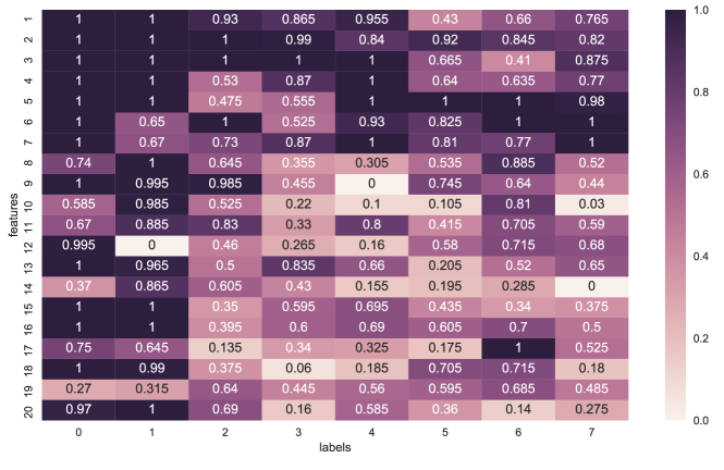
Figure 8. AS-733 Graph. Rows are the node of which ABC value is used as classifier. Columns are the classes(labels), that is, top 7 nodes being disconnected from the network one-by-one. Observing top i-th node’s (y-axis) ABC value helps classify the top i-th node’s (x-axis) removal. Class (label) 0 is the graph when there is no change.

5.3. Effect of Noise in Experiments

It is imperative to consider external/natural factors. Not every node on the communication graph behaves the same all the time. We achieve this in our experiments by incorporating noise factor to the communication probabilities. While each node initiates communication with others proportional to its initiator (sender) probability, and receives communication proportional to its receiver probability, these should be varying from time to time (between intervals) so that we do not assume that every node behaves exactly the same all the time. For our experiments, we have added a multiplicative noise factor uniformly random in the 0.8–1.2 range to the communication probability of the nodes.

The cardinality algorithm inherently is not affected by the noise since that is what we actually want to compute: The active usage and its effective centrality instead of static structure.

However, the empirical use cases we provided slightly deteriorate in the face of noisy data. In our experiments, we saw that for the AS-733 and Airports graphs, the accuracy decreased by 10% on average and up to 35% for same labels in AS-733 graph.

Overall, the algorithms are still able to successfully detect changes in most cases. More sophisticated detection approaches can be implemented to further improve quality and make it even more robust to noise, however, this is not in the scope of this paper.

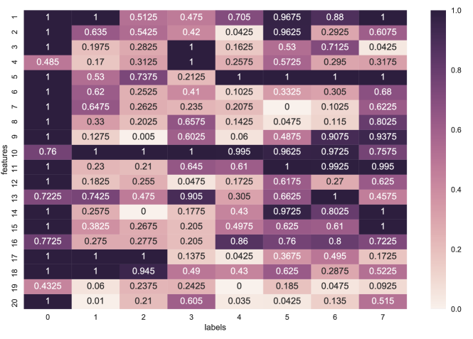
Figure 9. Airports Graph Rows are the node of which ABC value is used as classifier. Columns are the classes(labels), that is, top 7 nodes being disconnected from the network one-by-one. Observing top i-th node’s (y-axis) ABC value helps classify the top i-th node’s (x-axis) removal. Class (label) 0 is the graph when there is no change.

6. Conclusion and Discussion

Detection of critical nodes of a graph has become one of the main starting points for any graph analysis algorithm. Many importance measures (such as betweenness and closeness centrality) have been developed for the purpose of providing insights for node criticality. These measures rely on two assumptions, (i) centrality of a node depends only on the the structure of the graph and do not take the network activity into account. (ii) the exact graph structure is known. These assumptions limit the applicability of these methods. In this work, we have introduced a new metric, active betweenness cardinality, which can takes into account network activity while assessing criticality and does not require knowing of the exact topology. We showed how this metric can be computed efficiently and how most critical nodes can be identified. We empirically show that the metric can be used to detect significant changes in the topology of the network robustly.

References

- (1)
- Bader et al. (2007) David A. Bader, Shiva Kintali, Kamesh Madduri, and Milena Mihail. 2007. Approximating Betweenness Centrality. In Proceedings of the 5th International Conference on Algorithms and Models for the Web-graph (WAW’07). Springer-Verlag, Berlin, Heidelberg, 124–137. http://dl.acm.org/citation.cfm?id=1777879.1777889
- Boldi and Vigna (2013) Paolo Boldi and Sebastiano Vigna. 2013. In-Core Computation of Geometric Centralities with HyperBall: A Hundred Billion Nodes and Beyond. CoRR abs/1308.2144 (2013). arXiv:1308.2144 http://arxiv.org/abs/1308.2144
- Brandes (2001) Ulrik Brandes. 2001. A Faster Algorithm for Betweenness Centrality. Journal of Mathematical Sociology 25, 2 (2001), 163–177.
- Charikar et al. (2002) Moses Charikar, Kevin Chen, and Martin Farach-Colton. 2002. Finding frequent items in data streams. Automata, languages and programming (2002), 784–784.
- Chung and Lu (2002) Fan Chung and Linyuan Lu. 2002. The average distances in random graphs with given expected degrees. Proceedings of the National Academy of Sciences 99, 25 (2002), 15879–15882.
- Cohen (2015) Edith Cohen. 2015. All-distances sketches, revisited: HIP estimators for massive graphs analysis. IEEE Transactions on Knowledge and Data Engineering 27, 9 (2015), 2320–2334.
- Dekker (2005) Anthony Dekker. 2005. Conceptual Distance in Social Network Analysis. Journal of Social Structure 6, 3 (2005).
- Durand and Flajolet (2003) Marianne Durand and Philippe Flajolet. 2003. Loglog counting of large cardinalities. In European Symposium on Algorithms. Springer, 605–617.
- Flajolet et al. (2007) Philippe Flajolet, Éric Fusy, Olivier Gandouet, and Frédéric Meunier. 2007. Hyperloglog: the analysis of a near-optimal cardinality estimation algorithm. In AofA: Proceedings of the 2017 International Conference on Analysis of Algorithms. Discrete Mathematics and Theoretical Computer Science, 137–156.
- Flajolet and Martin (1985) Philippe Flajolet and G. Nigel Martin. 1985. Probabilistic counting algorithms for data base applications. J. Comput. System Sci. 31, 2 (1985), 182 – 209. https://doi.org/10.1016/0022-0000(85)90041-8
- Freeman (1977) Linton C. Freeman. 1977. A Set of Measures of Centrality Based on Betweenness. Sociometry 40, 1 (1977), 35–41. http://www.jstor.org/stable/3033543
- Heule et al. (2013) Stefan Heule, Marc Nunkesser, and Alexander Hall. 2013. HyperLogLog in Practice: Algorithmic Engineering of a State of the Art Cardinality Estimation Algorithm. In Proceedings of the 16th International Conference on Extending Database Technology (EDBT ’13). ACM, New York, NY, USA, 683–692. https://doi.org/10.1145/2452376.2452456
- Jia et al. (2011) Yuntao Jia, Victor Lu, Jared Hoberock, Michael Garland, and John C Hart. 2011. Edge v. node parallelism for graph centrality metrics. GPU Computing Gems 2 (2011), 15–30.
- Jin et al. (2010) Shuangshuang Jin, Zhenyu Huang, Yousu Chen, Daniel G. Chavarría-Miranda, John Feo, and Pak Chung Wong. 2010. A novel application of parallel betweenness centrality to power grid contingency analysis. In Proceedings of IEEE International Parallel and Distributed Processing Symposium (IPDPS). 1–7.
- Katz (1953) Leo Katz. 1953. A new status index derived from sociometric analysis. Psychometrika 18, 1 (1953), 39–43.
- Leskovec and Krevl (2014) Jure Leskovec and Andrej Krevl. 2014. SNAP Datasets: Stanford Large Network Dataset Collection. http://snap.stanford.edu/data. (June 2014).
- Madduri et al. (2009) Kamesh Madduri, David Ediger, Karl Jiang, David A. Bader, and Daniel G. Chavarría-Miranda. 2009. A faster parallel algorithm and efficient multithreaded implementations for evaluating betweenness centrality on massive datasets. In 23rd International Symposium on Parallel and Distributed Processing, Workshops and PhD Forum (IPDPSW), Workshop on Multithreaded Architectures and Applications (MTAAP).
- Malkin (1998) Gary Scott Malkin. 1998. RIP Version 2. STD 56. RFC Editor. http://www.rfc-editor.org/rfc/rfc2453.txt http://www.rfc-editor.org/rfc/rfc2453.txt.
- Merrer and Trédan (2009) Erwan Le Merrer and Gilles Trédan. 2009. Centralities: Capturing the Fuzzy Notion of Importance in Social Graphs. In Proceedings of the Second ACM EuroSys Workshop on Social Network Systems (SNS).
- Meyers et al. (2006) Lauren Ancel Meyers, MEJ Newman, and Babak Pourbohloul. 2006. Predicting epidemics on directed contact networks. Journal of theoretical biology 240, 3 (2006), 400–418.
- Opsahl et al. (2010) Tore Opsahl, Filip Agneessens, and John Skvoretz. 2010. Node Centrality in Weighted Networks: Generalizing Degree and Shortest Paths. Social Networks 3, 32 (2010), 245–251.
- Pande and Bader (2011) P Pande and David A Bader. 2011. Computing betweenness centrality for small world networks on a GPU. In 15th Annual High Performance Embedded Computing Workshop (HPEC).
- Pedregosa et al. (2011) Fabian Pedregosa, Gaël Varoquaux, Alexandre Gramfort, Vincent Michel, Bertrand Thirion, Olivier Grisel, Mathieu Blondel, Peter Prettenhofer, Ron Weiss, Vincent Dubourg, et al. 2011. Scikit-learn: Machine learning in Python. Journal of Machine Learning Research 12, Oct (2011), 2825–2830.
- Pham and Klamma (2010) Manh Cuong Pham and Ralf Klamma. 2010. The Structure of the Computer Science Knowledge Network. In Proceedings of International Conference on Advances in Social Networks Analysis and Mining (ASONAM).
- Priest and Cybenko (2017) Benjamin W. Priest and George Cybenko. 2017. Approximating centrality in evolving graphs: toward sublinearity. (2017), 10184 - 10184 - 9 pages. https://doi.org/10.1117/12.2266376
- Riondato and Kornaropoulos (2014) Matteo Riondato and Evgenios M. Kornaropoulos. 2014. Fast Approximation of Betweenness Centrality Through Sampling. In Proceedings of the 7th ACM International Conference on Web Search and Data Mining (WSDM ’14). ACM, New York, NY, USA, 413–422. https://doi.org/10.1145/2556195.2556224
- Riondato and Upfal (2016) Matteo Riondato and Eli Upfal. 2016. ABRA: Approximating Betweenness Centrality in Static and Dynamic Graphs with Rademacher Averages. In Proceedings of the 22Nd ACM SIGKDD International Conference on Knowledge Discovery and Data Mining (KDD ’16). ACM, New York, NY, USA, 1145–1154. https://doi.org/10.1145/2939672.2939770
- Rochat (2009) Yannick Rochat. 2009. Closeness centrality extended to unconnected graphs: The harmonic centrality index. Applications of Social Network Analysis (2009).
- Sarıyüce et al. (2013) Ahmet Erdem Sarıyüce, Kamer Kaya, Erik Saule, and Ümit V. Çatalyürek. 2013. Betweenness Centrality on GPUs and Heterogeneous Architectures. In Workshop on General Purpose Processing Using GPUs (GPGPU), in conjunction with ASPLOS.
- Sarıyüce et al. (2015) Ahmet Erdem Sarıyüce, Erik Saule, Kamer Kaya, and Ümit V. Çatalyürek. 2015. Regularizing Graph Centrality Computations. J. Parallel Distrib. Comput. 76, C (Feb. 2015), 106–119.
- Shi and Zhang (2011) Zhiao Shi and Bing Zhang. 2011. Fast network centrality analysis using GPUs. BMC Bioinformatics 12 (2011), 149.
- Şimşek and Barto (2009) Özgür Şimşek and Andrew G Barto. 2009. Skill characterization based on betweenness. In Advances in neural information processing systems. 1497–1504.