Notes on Fano Ratio and Portfolio Optimization

Zura Kakushadze^§† and Willie Yu^♯

^§ Quantigic^® Solutions LLC

1127 High Ridge Road #135, Stamford, CT 06905  

^† Free University of Tbilisi, Business School & School of Physics

240, David Agmashenebeli Alley, Tbilisi, 0159, Georgia

^♯ Centre for Computational Biology, Duke-NUS Medical School

8 College Road, Singapore 169857

(October 9, 2017)

We discuss – in what is intended to be a pedagogical fashion – generalized “mean-to-risk” ratios for portfolio optimization. The Sharpe ratio is only one example of such generalized “mean-to-risk” ratios. Another example is what we term the Fano ratio (which, unlike the Sharpe ratio, is independent of the time horizon). Thus, for long-only portfolios optimizing the Fano ratio generally results in a more diversified and less skewed portfolio (compared with optimizing the Sharpe ratio). We give an explicit algorithm for such optimization. We also discuss (Fano-ratio-inspired) long-short strategies that outperform those based on optimizing the Sharpe ratio in our backtests.

1 Introduction and Summary

When constructing a (e.g., stock) portfolio, one balances risk and reward (i.e., expected return) [Sharpe, 1966]. Mean-variance optimization [Markowitz, 1952] provides an implementation of this general idea. In some (somewhat limited) sense, maximizing the Sharpe ratio [Sharpe, 1966] can be taken as a justification for mean-variance optimization. Thus, without costs, bounds, constraints, etc., maximizing the Sharpe ratio of a portfolio is equivalent to mean-variance optimization. However, once, e.g., costs are included, this equivalence is gone. This begs the question:

Can we anchor portfolio optimization on quantities other than the Sharpe ratio? In these notes we address precisely this question. The Sharpe ratio is a ratio of the (properly adjusted – see below) expected return over the standard deviation. So, it is a ratio of the expected return to a particular measure of risk, in this case, the standard deviation. However, we can consider other measures of risk, e.g., some generic function of the variance. Thus, one property of the Sharpe ratio is that it depends on the time horizon for which it is calculated. E.g., a daily expected return and volatility give us a daily Sharpe ratio, which is on average lower (by a factor of $\sqrt{252}$, where 252 is the approximate number of trading days in a year, if we focus on stocks) than an annualized Sharpe ratio. If the daily expected return and volatility are stable in time, the Sharpe ratio goes to infinity as $\sqrt{T}$ with the time horizon $T$.

In contrast, the mean-to-variance ratio (i.e., the expected-return-to-variance ratio) – which we refer to as the Fano ratio (see the next section) – is independent of the horizon $T$ (in the aforementioned sense). We could then take the Fano ratio as the starting point for portfolio optimization. As mentioned above, more generally, we can take a ratio of the expected return to a suitable function of the variance. This is the avenue we explore in these notes, which are intended to be pedagogical.

In Section 2 we discuss maximizing generalized mean-to-risk ratios in the context of long-only portfolios. Maximizing the Fano ratio leads to simplifications (compared with the general case). Dealing with nonnegativity of the portfolio weights, just as when maximizing the Sharpe ratio, requires an iterative procedure and we provide an approximate relaxation algorithm for optimizing the Fano ratio. For long-only portfolios optimizing the Fano ratio effectively amounts to shifting the expected returns by a positive amount, which results in fewer stocks being excluded from the portfolio (including some stocks with negative expected returns), i.e., in a more diversified and less skewed portfolio (compared with optimizing the Sharpe ratio).

In Section 3 we discuss long-short portfolios, for which certain issues with optimizing the Fano ratio inspire construction of new “multiply-optimized” strategies, which outperform optimizing the Sharpe ratio. We briefly conclude in Section 4.

2 Generalized Mean-to-Risk Ratios

Our discussion below is agnostic to the underlying tradable instruments, which a priori can be stocks, bonds, currencies, etc. However, for the sake of definiteness, let us focus on a portfolio of stocks (e.g, 2,000+ most liquid U.S. stocks). So, we have $N$ stocks with time series of (e.g., close-to-close daily, weekly, monthly or some other horizon) returns $R_{is}$, $i=1,\dots,N$. Here the index $s=1,\dots,T$ labels trading days on which these returns are computed ($s=1$ labels the most recent date).

Above, $R_{is}$ are the realized returns (ex-post). We can also define expected returns (ex-ante) via, e.g., moving averages:

$$E_{is}={1\over d}\sum_{s^{\prime}=s+1}^{s+d}R_{is^{\prime}}$$ (1)

Thus, if $R_{is}$ are daily returns, then $E_{is}$ are $d$-day moving averages. We emphasize that (1) is only an example and there are myriad other ways of constructing $E_{is}$. Generally, expected returns can be quite convoluted and have no simple financial interpretation, e.g., machine learning based expected returns [Kakushadze, 2016]. In the following, for the sake of simplicity, we will omit the index $s$ and refer to expected returns as $E_{i}$. Thus, we can think of $E_{i}$ as the expected returns for $s=1$ (i.e., “today’s” date). What is important is that $E_{i}$ are computed out-of-sample.

Next, we can define a sample covariance matrix $C_{ij}$ based on the time series $E_{is}$ or $R_{is}$ and also computed out-of-sample (ex-ante). In what follows it may appear natural to compute $C_{ij}$ based on the expected returns $E_{is}$ as opposed to the realized returns $R_{is}$. However, in practice, in many cases it can be (much) simpler to compute $C_{ij}$ based on $R_{is}$. In some cases basing $C_{ij}$ on $E_{is}$ may not even be practicable. One issue is that typically the lookback – i.e., the number of datapoints in the time series, call it $M$ – is insufficient to compute $C_{ij}$ reliably. Thus, if $M<N+1$, then the sample covariance matrix $C_{ij}$ is singular, whereas for our purposes below $C_{ij}$ must be positive-definite. Furthermore, unless $M\gg N$, which is rarely if ever the case in practice, the off-diagonal elements (in particular, the correlations – the diagonal elements are relatively stable) are highly unstable out-of-sample rendering $C_{ij}$ essentially useless (unpredictive out-of-sample). So, in practice one replaces the sample covariance matrix $C_{ij}$ via a model covariance matrix, call it $\Gamma_{ij}$, such as a multifactor risk model. If built in-house, $\Gamma_{ij}$ could a priori be built based on $E_{is}$ (among other things). If it is a third-party product, naturally, it is built based on $R_{is}$ (or some other returns). In any event, here we will not delve into how $\Gamma_{ij}$ is built. We will simply assume that $C_{ij}$ below is identified with some model covariance matrix $\Gamma_{ij}$, which is i) positive-definite and ii) sufficiently stable out-of-sample.

2.1 Generalized Mean-to-Risk Ratios for Portfolios

Now we can define portfolio risk. Let us assume that our portfolio consists of our $N$ stocks with weights $w_{i}$. A priori some of these weights can be 0 or negative. The normalization condition for the weights is

$$\sum_{i=1}^{N}|w_{i}|=1$$ (2)

Below we will consider a case with nonnegative weights; for now $w_{i}$ are general.

The expected return of the portfolio is given by

$$E=\sum_{i=1}^{N}w_{i}~{}E_{i}$$ (3)

The expected variance of the portfolio is given by

$$V=\sum_{i,j=1}^{N}C_{ij}~{}w_{i}~{}w_{j}$$ (4)

We can define the Sharpe ratio [Sharpe, 1994] of the portfolio via

$$S={E\over\sqrt{V}}$$ (5)

A nice thing about the Sharpe ratio is that it is invariant under the formal rescalings $w_{i}\rightarrow\zeta~{}w_{i}$, where $\zeta>0$. This rescaling invariance is the reason why in the absence of trading costs, bounds, etc., maximizing the Sharpe ratio is equivalent to mean-variance optimization [Markowitz, 1952]. Indeed, maximizing (5) (i.e., we find the maximum of $S$ w.r.t. $w_{i}$) is equivalent to maximizing (w.r.t. $w_{i}$) the objective function

$$g=E-{\lambda\over 2}~{}V$$ (6)

and $\lambda$ is fixed (after maximization) via (2). So, in some (somewhat limited) sense, maximizing the Sharpe ratio can be taken as a justification for mean-variance optimization. However, once, e.g., trading costs, etc., are added, maximizing the Sharpe ratio is no longer equivalent to mean-variance optimization [Kakushadze, 2015a].

Furthermore, one property of the Sharpe ratio is that it depends on the time horizon for which it is calculated. E.g., a daily expected return and volatility give us a daily Sharpe ratio, which is on average lower (by a factor of $\sqrt{d}$, where $d\approx 252$ is the approximate number of trading days in a year, if we focus on stocks) than an annualized Sharpe ratio. If the daily expected return and volatility do not change much in time, then the Sharpe ratio goes to infinity as $\sqrt{T}$ with the time horizon $T$. So, a practical way of thinking about the Sharpe ratio is that, if, say, the annualized Sharpe ratio is 2, then the probability of losing money in a given year is less than about 2.3% (assuming normally distributed realized returns, that is, which can be farfetched – see below). Can we define a ratio independent of the time horizon?

The answer is affirmative. We can simply define the mean-to-variance ratio:

$$F={E\over V}$$ (7)

This ratio is independent of the horizon $T$ (in the aforementioned sense). Other than tautological “mean-to-variance ratio”, this ratio apparently has not been named in finance. It would appear appropriate to term it the Fano ratio due to its relationship to the Fano factor [Fano, 1947] named after Ugo Fano, an Italian American physicist. The Fano factor (a.k.a. variance-to-mean ratio and index of dispersion), in our notations, is simply $V/E$, i.e., the inverse of the Fano ratio (7). Up to a factor of 2, it is the same as the ratio

$$\kappa={2E\over V}$$ (8)

discussed in [Kakushadze, 2017] in the context of stock price bubbles, where it was argued that the dimensionless ratio $\kappa$ can be used to define a criterion for when a stock (or a similar instrument) is not a good investment in the long term, which can happen even if the expected return is positive. Thus, assuming log-normal distribution for stock prices, this criterion (i.e., that the stock is not a good investment in a long run) is

$$\kappa<1$$ (9)

This criterion for the Fano ratio (defined for a single stock) would be $F<1/2$.

So, naturally, we can ask: why not maximize the Fano ratio (instead of the Sharpe ratio)? In fact, we can define more general “mean-to-risk” ratios via

$$G={E\over f(V)}$$ (10)

where $f(V)$ is some function of $V$. We can then maximize $G$ instead of $S$ (or $F$).

Recall, however, that we could ignore the normalization condition (2) when maximizing the Sharpe ratio as the latter is invariant under the rescalings $w_{i}\rightarrow\zeta~{}w_{i}$. Such invariance is gone in the case of the Fano ratio or more general ratios $G$ defined via (10). So, the maximization problem becomes more nontrivial. Thus, we must maximize the objective function

$$g=G+\mu\left(\sum_{i=1}^{N}|w_{i}|-1\right)$$ (11)

where $\mu$ is a Lagrange multiplier. The modulus complicates things quite a bit (see Section 3). Therefore, for the sake of simplicity, for now let us focus on the case of long-only portfolios, where $w_{i}\geq 0$. Then our objective function simplifies:

$$g=G+\mu\left(\sum_{i=1}^{N}w_{i}-1\right)$$ (12)

However, now we have bounds

$$w_{i}\geq 0$$ (13)

To get a flavor of the problem at hand, at first we will ignore the bounds (13) when solving the maximization problem and then incorporate them via a certain trick.

2.2 Maximization Ignoring Bounds

Maximizing (12) w.r.t. $w_{i}$ and $\mu$ (and ignoring the bounds (13)), we get the following solution ($f^{\prime}(V)$ is the first derivative w.r.t. $V$, and $C^{-1}_{ij}$ is the inverse of $C_{ij}$):

$$w_{i}=a~{}{\widehat{\eta}}_{i}+b~{}{\widehat{\nu}_{i}}$$ (14)

$${\widehat{\eta}}_{i}=\sum_{j=1}^{N}C^{-1}_{ij}~{}E_{j}$$ (15)

$${\widehat{\nu}}_{i}=\sum_{j=1}^{N}C^{-1}_{ij}~{}\nu_{j}$$ (16)

$$a={f(V)\over 2Ef^{\prime}(V)}$$ (17)

$$b=V-{f(V)\over 2f^{\prime}(V)}$$ (18)

Here $\nu_{i}\equiv 1$ is the unit $N$-vector (using which might appear redundant at first, but will be useful later). So, we have three unknowns, $E$, $V$ and $a$. Using the condition $\sum_{i=1}^{N}w_{i}=1$ and the definitions (3) and (4), we have the following equations:

$$a\gamma+b\beta^{2}=1$$ (19)

$$E=a\alpha^{2}+b\gamma$$ (20)

$$V=a^{2}\alpha^{2}+2ab\gamma+b^{2}\beta^{2}=a^{2}\alpha^{2}+(a\gamma+1)b=a^{2}\alpha^{2}+(1-a^{2}\gamma^{2})/\beta^{2}$$ (21)

where

$$\alpha^{2}=\sum_{i,j=1}^{N}C^{-1}_{ij}~{}E_{i}~{}E_{j}$$ (22)

$$\beta^{2}=\sum_{i,j=1}^{N}C^{-1}_{ij}~{}\nu_{i}~{}\nu_{j}$$ (23)

$$\gamma=\sum_{i,j=1}^{N}C^{-1}_{ij}~{}E_{i}~{}\nu_{j}$$ (24)

and in (21) we repeatedly used (19). So we can express $a$ via $V$:

$$a^{2}={{V\beta^{2}-1}\over{\alpha^{2}\beta^{2}-\gamma^{2}}}$$ (25)

Combining (19), (18) and (25), we get the following equation involving $V$ only:

$$\gamma^{2}~{}{{V\beta^{2}-1}\over{\alpha^{2}\beta^{2}-\gamma^{2}}}=\left(1+\beta^{2}\left[{f(V)\over 2f^{\prime}(V)}-V\right]\right)^{2}$$ (26)

For general $f(V)$ this equation is transcendental. In some cases it simplifies.

Let us start with the case of the Sharpe ratio $f(V)=\sqrt{V}$. Then we have the familiar solution $b=0$ and $a=1/\gamma$. If $f(V)=V^{p}$, where $p>0$ and $p\neq 1/2$, then (26) is a quadratic equation for $V$ and can be readily solved. It is also a quadratic equation when $f(V)=\exp(\xi V)$. For $f(V)=\exp(\xi V^{2})$ the equation is quartic.

2.2.1 Maximizing Fano Ratio

While the aforesaid quadratic equations can be solved, generally they involve radicals and are not particularly illuminating. However, in the case of the Fano ratio, i.e., when $f(V)=V$, things further simplify and there are no radicals. The solution is:

$$a={1\over{\alpha\beta+\gamma}}$$ (27)

$$b={\alpha\over{\beta(\alpha\beta+\gamma)}}$$ (28)

and we have

$$E={\alpha\over\beta}$$ (29)

$$V={2\alpha\over{\beta(\alpha\beta+\gamma)}}$$ (30)

$$F={1\over 2}\left(\alpha\beta+\gamma\right)$$ (31)

$$S=\sqrt{\alpha(\alpha\beta+\gamma)\over 2\beta}$$ (32)

Had we maximized the Sharpe ratio, we would get $E_{*}=\alpha^{2}/\gamma$, $V_{*}=\alpha^{2}/\gamma^{2}$, $F_{*}=\gamma$ and $S_{*}=\alpha$. Since $\gamma<\alpha\beta$, it follows that $S<S_{*}$ and $F>F_{*}$ (which should come as no surprise as $F$ and $S_{*}$ are the maximum possible values thereof), and $E<E_{*}$ and $V<V_{*}$. So, maximizing the Fano ratio produces a portfolio with a lower expected return but also a lower expected volatility than maximizing the Sharpe ratio.

2.3 Incorporating Bounds

The solution (14) is not necessarily good in the sense that some $w_{i}$ might be negative. Indeed, even if all $E_{i}$ are nonnegative, we can have negative $w_{i}$ due to the off-diagonal elements in $C_{ij}$. So, we must incorporate the bounds (13) into the solution somehow.

The issue is that we are not dealing with a quadratic optimization problem here. However, not all is lost and the following trick provides a reasonable approximation. Thus, the solution (14) formally can be thought of as the solution to maximizing the following quadratic objective function ($\lambda$ is fixed after solving for $w_{i}$ by rescaling them such that $\sum_{i=1}^{N}w_{i}=1$, which rescaling is not affected by the bounds (13))

$${\widetilde{g}}={\widetilde{E}}-{\lambda\over 2}~{}V$$ (33)

subject to the bounds (13), where (note that $\lambda=\alpha(J)\beta(J)+\gamma(J)$)

$${\widetilde{E}}=\sum_{i=1}^{N}w_{i}~{}{\widetilde{E}}_{i}$$ (34)

$${\widetilde{E}}_{i}=E_{i}+E(J)~{}\nu_{i}$$ (35)

$$E(J)={\alpha(J)\over\beta(J)}$$ (36)

$$[\alpha(J)]^{2}=\sum_{i,j\in J}[C(J)]^{-1}_{ij}~{}E_{i}~{}E_{j}$$ (37)

$$[\beta(J)]^{2}=\sum_{i,j\in J}[C(J)]^{-1}_{ij}~{}\nu_{i}~{}\nu_{j}$$ (38)

$$\gamma(J)=\sum_{i,j\in J}[C(J)]^{-1}_{ij}~{}E_{i}~{}\nu_{j}$$ (39)

where $J=\{i|w_{i}>0\}$ is the subset of positive weights, $[C(J)]^{-1}_{ij}$ is the $N(J)\times N(J)$ matrix inverse to the $N(J)\times N(J)$ matrix $[C(J)]_{ij}$ obtained from $C_{ij}$ by restricting $i,j\in J$. (Here $N(J)=|J|$ is the number of elements in $J$.) So, the catch is that $E(J)$, and thereby ${\widetilde{E}}_{i}$, depend on $J$, which is unknown. Had $E(J)$ been known a priori, then we would simply minimize (33) subject to the bounds (13) via standard quadratic optimization techniques. So, here is a relaxation algorithm that approximates the optimal solution. At the initial iteration, we assume that $J^{(0)}$ is the full set $\{1,\dots,N\}$ and compute $w_{i}$ via (14). If all $w_{i}\geq 0$, then there is nothing else to do, we are done. So, let us assume that the set ${\widetilde{J}}^{(0)}=\{i|w_{i}<0\}$ is not empty. Let us take the value of $\ell\in{\widetilde{J}}^{(0)}$ for which $F_{\ell}=\min(F_{i})$, where $F_{i}=E_{i}/C_{ii}$ are the Fano ratios for each stock. We then permanently set $w_{\ell}=0$, take $J^{(1)}=J^{(0)}\setminus\ell$ and compute $w_{i}$ via (14). If the resulting $w_{i}\geq 0$ for all $i\in J^{(1)}$, then we are done. So, let us assume that the set ${\widetilde{J}}^{(1)}=\{i|w_{i}<0,i\in J^{(1)}\}$ is not empty. Let us take the value of $\ell^{\prime}\in{\widetilde{J}}^{(1)}$ for which $F_{\ell^{\prime}}=\min(F_{i})$, $i\in J^{(1)}$ (see fn.18). We then permanently set $w_{\ell^{\prime}}=0$, take $J^{(2)}=J^{(1)}\setminus\ell^{\prime}$ and compute $w_{i}$ via (14). And so on. We repeat this procedure until at some $k$-th iteration all $w_{i}\geq 0$ for $i\in J^{(k)}$. As always, one issue with this relaxation algorithm is the computational cost: we must compute the inverse matrix $[C(J)]^{-1}_{ij}$ at each iteration. However, for a $K$-factor model of the form (here $\xi_{i}^{2}$ is the specific a.k.a. idiosyncratic risk, $\Omega_{iA}$, $A=1,\dots,K$ is the factor loadings matrix, and $\phi_{AB}$ is the factor covariance matrix)

$$C_{ij}=\xi_{i}^{2}~{}\delta_{ij}+\sum_{A,B=1}^{K}\Omega_{iA}~{}\phi_{AB}~{}\Omega_{jB}$$ (40)

to compute $[C(J)]^{-1}_{ij}$, we only need to invert the $K\times K$ matrix $\phi_{AB}$ once, plus we must invert a $K\times K$ matrix

$$[Q(J)]_{AB}=\phi^{-1}_{AB}+\sum_{i\in J}{1\over\xi_{i}^{2}}~{}\Omega_{iA}~{}\Omega_{iB}$$ (41)

at each iteration. However, these inversions are much cheaper assuming $K\ll N$.

2.4 The “Market” Mode

The issue we wish to address next is equally pertinent to maximizing the Sharpe ratio, the Fano ratio and the generalized mean-to-risk ratios we discuss above. For the sake of definiteness and simplicity, let us focus on the case of maximizing the Sharpe ratio. Let us ignore the bounds (13) for a moment. Then the weights are given by

$$w_{i}=a~{}\sum_{j=1}^{N}C^{-1}_{ij}~{}E_{j}$$ (42)

$$a^{-1}=\sum_{i,j=1}^{N}C^{-1}_{ij}~{}E_{i}~{}\nu_{j}$$ (43)

For a typical configuration, even if all $E_{i}$ are nonnegative, close to 50% of the weights $w_{i}$ can be negative. Thus, to illustrate this point, let us consider the following “toy” covariance matrix: $C_{ij}=\sigma_{i}\sigma_{j}\Psi_{ij}$, where $\sigma_{i}^{2}$ are the variances; the correlation matrix $\Psi_{ij}=\left(1-\rho\right)\delta_{ij}+\rho\nu_{i}\nu_{j}$; and $\nu_{i}\equiv 1$ is the unit $N$-vector. I.e., all $N$ stocks have uniform pair-wise correlations equal $\rho$. Inverting this matrix gives the following weights:

$$w_{i}={a\over\sigma_{i}\left(1-\rho\right)}\left[{\widetilde{E}}_{i}-{\rho~{}\nu_{i}\over{1+(N-1)\rho}}~{}\sum_{j=1}^{N}{\widetilde{E}}_{j}\right]$$ (44)

where ${\widetilde{E}}_{i}=E_{i}/\sigma_{i}$ are the normalized expected returns. Generically, the latter are expected to be roughly symmetrically distributed around their mean. It is then evident from (44) that, unless $\rho\ll 1/N$, roughly 50% of the weights $w_{i}$ are negative.

Now, in practice the correlation matrix with uniform pair-wise correlations is unrealistic. However, the above issue persists even for realistic correlation matrices. Thus, consider a general correlation matrix $\Psi_{ij}$. We can always write it as

$$\Psi_{ij}=\left(1-\rho\right)\delta_{ij}+\rho\nu_{i}\nu_{j}+\Delta_{ij}=\Psi^{\prime}+\Delta_{ij}$$ (45)

Here $\rho={1\over N(N-1)}\sum_{i,j=1;~{}i\neq j}^{N}\Psi_{ij}$ is the average pair-wise correlation, and $\sum_{i,j=1}^{N}\Delta_{ij}=0$. In the zeroth approximation we can drop $\Delta_{ij}$, i.e., $\Psi_{ij}\approx\Psi^{\prime}_{ij}$. Its first principal component $U^{(1)}_{i}=\nu_{i}/\sqrt{N}$. It describes the “market” mode [Bouchaud and Potters, 2011], i.e., the average correlation of all stocks, which is nonzero (and not small, definitely $\rho\not\ll 1/N$). The “market” mode corresponds to the overall movement of the broad market, which affects all stocks (to varying degrees) – cash inflow (outflow) into (from) the market tends to push stock prices higher (lower). This is the market risk factor. To mitigate this risk factor, one can, e.g., hold a dollar-neutral portfolio of stocks. However, long-only portfolios are exposed to market risk by construction.

So, neutralizing the market risk factor while maximizing the Sharpe ratio is an unwelcome feature. Why? Because at the end we impose the bounds (13) anyway, so the market risk is still present, but the resultant portfolio gets artificially distorted due to pushing the negative weights (that is, in the unbounded optimization) to zero thereby also affecting the positive weights. The culprit here is that, when maximizing the Sharpe ratio using a covariance matrix that includes the “market” mode, we approximately neutralize the portfolio w.r.t. the market risk. Put differently, we hedge against all stocks – i.e., the broad market – going bust. However, holding a long-only portfolio with thousands of stocks invariably is exposed to the broad market. So, we must eliminate the “market” mode out of the covariance matrix.

In the context of factor models (40) this can be achieved relatively easily. In this case (ignoring the bounds (13)) we have (as above, $a$ is fixed via $\sum_{i=1}^{N}w_{i}=1$)

$$w_{i}=a~{}\left[{E_{i}\over\xi_{i}^{2}}-{1\over\xi_{i}^{2}}~{}\sum_{A,B=1}^{K}\Omega_{iA}~{}Q^{-1}_{AB}~{}\sum_{j=1}^{N}{E_{j}\over\xi_{j}^{2}}~{}\Omega_{jB}\right]$$ (46)

$$Q_{AB}=\phi^{-1}_{AB}+\sum_{i=1}^{N}{1\over\xi_{i}^{2}}~{}\Omega_{iA}~{}\Omega_{iB}$$ (47)

Eliminating the “market” mode from $C_{ij}$ then amounts to requiring that the factor loadings matrix is orthogonal to some positive $N$-vector $v_{i}>0$:

$$\sum_{i=1}^{N}v_{i}~{}\Omega_{iA}\equiv 0$$ (48)

Then we no longer have roughly 50% of negative weights $w_{i}$. While some of these weights can still be negative, typically the number of such negative weights will be relatively small compared with $N$ (assuming all $E_{i}\geq 0$, that is). So, what are $v_{i}$?

One – but not the only – way of thinking about $v_{i}$ is that they are the weights of some benchmark long-only portfolio: $v_{i}=w^{benchmark}_{i}>0$. The choice of this benchmark portfolio is not all that critical provided it is reasonably diversified. For example, we can take $v_{i}\equiv 1$, i.e., an equally-weighted benchmark. We can take $v_{i}=1/\sigma_{i}^{2}$ or $v_{i}=1/\xi_{i}^{2}$. This can skew the portfolio toward low-volatility (which are typically large market cap) stocks. To mitigate this, we can Windsorize or otherwise deal with the tails in the skewed (roughly log-normal) distribution of $\sigma_{i}$ (or $\xi_{i}$). Etc.

2.5 Statistical Risk Models

Statistical risk models [Kakushadze and Yu, 2017b] provide a particularly simple example of factor models, where the factor covariance matrix is diagonal. Thus, let $\Psi^{sample}_{ij}$ be the sample correlation matrix computed based on time series of historical returns. $\Psi^{sample}_{ij}$ can be singular. This will not affect our discussion below. The sample covariance matrix is $C^{sample}_{ij}=\sigma_{i}\sigma_{j}\Psi^{sample}_{ij}$. We can construct a statistical risk model covariance matrix $C_{ij}$ as follows:

$$C_{ij}=\sigma_{i}\sigma_{j}\Psi_{ij}$$ (49)

$$\Psi_{ij}={\widetilde{\xi}}_{i}^{2}~{}\delta_{ij}+\sum_{a=1}^{K}\lambda^{(a)}~{}V^{(a)}_{i}~{}V^{(a)}_{j}$$ (50)

$${\widetilde{\xi}}_{i}^{2}=1-\sum_{a=K+1}^{r}\lambda^{(a)}~{}[V^{(a)}_{i}]^{2}$$ (51)

Here $V^{(a)}_{i}$ are the principal components of the matrix $\Psi^{sample}_{ij}$ with the corresponding eigenvalues in the descending order: $\lambda^{(1)}>\lambda^{(2)}>\dots>\lambda^{(r)}$, where $r$ is the rank of $\Psi^{sample}_{ij}$ (if $r<N$, then for $a>r$ we have $\lambda^{(a)}=0$). The number of factors $K$ is determined via (truncated or rounded) eRank (effective rank) [Roy and Vetterli, 2007] – see [Kakushadze and Yu, 2017b] for details. The issue with the so-constructed $C_{ij}$ is that it contains the “market” mode. Indeed, without loss of generality we can assume that all elements of the first principal component $V^{(1)}_{i}>0$ – this can be ensured by, if need be, changing the basis as follows: $C_{ij}\rightarrow\epsilon_{i}\epsilon_{j}C_{ij}$, where $\epsilon_{i}=\mbox{sign}(V^{(1)}_{i})$. Then the all-positive $V^{(1)}_{i}$ can be regarded as the “market” mode [Bouchaud and Potters, 2011]. In fact, for large $N$ we have $V^{(1)}_{i}\approx 1/\sqrt{N}$. Note that higher principal components $V^{(a>1)}_{i}$ invariably have negative elements. So, we need to eliminate the first principal component. This can be achieved simply by defining

$$C_{ij}=\sigma_{i}\sigma_{j}{\widehat{\Psi}}_{ij}$$ (52)

$${\widehat{\Psi}}_{ij}={\widehat{\xi}}_{i}^{2}~{}\delta_{ij}+\sum_{a=2}^{K}\lambda^{(a)}~{}V^{(a)}_{i}~{}V^{(a)}_{j}$$ (53)

$${\widehat{\xi}}_{i}^{2}=1-\lambda^{(1)}~{}[V^{(1)}_{i}]^{2}-\sum_{a=K+1}^{r}\lambda^{(a)}~{}[V^{(a)}_{i}]^{2}$$ (54)

This is not the only possible definition, but it is as good as any other. With this definition we can think of the benchmark portfolio as that with $v_{i}=V^{(1)}_{i}/\sigma_{i}$.

Our discussion above is for maximizing the Sharpe ratio but equally applies to maximizing the Fano ratio and the generalized mean-to-risk ratios. This is because in all these cases the weights involve inverting the covariance matrix. Indeed, in (14) we have $w_{i}=a\sum_{j=1}^{N}C^{-1}_{ij}~{}E^{\prime}_{j}$, where $E^{\prime}_{i}=E_{i}+\nu_{i}~{}b/a$, so the above still applies.

2.6 Why Is This Useful?

For long-only portfolios optimizing the Fano ratio effectively amounts to shifting the expected returns by a positive amount via (35), which results in fewer stocks being excluded from the portfolio due to the bounds (13) (including some stocks with negative expected returns $E_{i}$, for which the effective returns ${\widetilde{E}}_{i}$ can be positive), i.e., in a more diversified and less skewed portfolio (compared with optimizing the Sharpe ratio). This is evident for a diagonal matrix $C_{ij}=\sigma_{i}^{2}~{}\delta_{ij}$. And this conclusion persists for non-diagonal $C_{ij}$ of the factor model form with the “market” mode removed. This can be illustrated using a simple 1-factor model of the form $C_{ij}=\sigma_{i}\sigma_{j}\Psi_{ij}$, where the correlation matrix $\Psi_{ij}=\left(1-\rho\right)\delta_{ij}+\rho s_{i}s_{j}$, and $s_{i}=1$ for half of the values of $i$, and $s_{i}=-1$ for the other half (the number of stocks $N$ is assumed to be even). (As above, let us ignore the bounds for a moment.) Then we have (here $a$ is given by (27))

$$w_{i}={a\over\sigma_{i}\left(1-\rho\right)}\left[{\widetilde{E}}^{\prime}_{i}-{\rho~{}s_{i}\over{1+(N-1)\rho}}~{}\sum_{j=1}^{N}{\widetilde{E}}^{\prime}_{j}~{}s_{j}\right]$$ (55)

$${\widetilde{E}}^{\prime}_{i}={\widetilde{E}}_{i}+{\alpha\over\beta}~{}{\nu_{i}\over\sigma_{i}}$$ (56)

$${\widetilde{E}}_{i}=E_{i}/\sigma_{i}$$ (57)

$$\alpha^{2}={1\over\left(1-\rho\right)}\left[\sum_{i=1}^{N}{\widetilde{E}}^{2}_{i}-{\rho\over{1+(N-1)\rho}}~{}\left(\sum_{i=1}^{N}{\widetilde{E}}_{i}~{}s_{i}\right)^{2}\right]$$ (58)

$$\beta^{2}={1\over\left(1-\rho\right)}\left[\sum_{i=1}^{N}{1\over\sigma_{i}^{2}}-{\rho\over{1+(N-1)\rho}}~{}\left(\sum_{i=1}^{N}{s_{i}\over\sigma_{i}}\right)^{2}\right]$$ (59)

It is reasonable to assume that there is no substantial correlation between the values of $\sigma_{i}$ and the signs $s_{i}$, or the values of $E_{i}$ and $s_{i}$. Then we can estimate that $\left|\sum_{i=1}^{N}s_{i}/\sigma_{i}\right|\mathrel{\hbox to0.0pt{\lower 3.0pt\hbox{\hskip 0.0pt$\sim$}\hss}\raise 1.0pt\hbox{$<$}}\sqrt{N}/\sigma_{*}$, where $N/\sigma_{*}^{2}=\sum_{i=1}^{N}1/\sigma_{i}^{2}$. Similarly, $\left|\sum_{i=1}^{N}{\widetilde{E}}_{i}~{}s_{i}\right|\mathrel{\hbox to0.0pt{\lower 3.0pt\hbox{\hskip 0.0pt$\sim$}\hss}\raise 1.0pt\hbox{$<$}}\sqrt{N}~{}{\widetilde{E}}_{*}$, where $N~{}{\widetilde{E}}_{*}^{2}=\sum_{i=1}^{N}{\widetilde{E}}_{i}^{2}$. Further, we can reasonably assume that $\rho\not\ll 1/N$ (and $N\gg 1$). Then we have

$$\alpha^{2}={N{\widetilde{E}}_{*}^{2}\over\left(1-\rho\right)}\left[1-{\cal O}(1/N)\right]$$ (60)

$$\beta^{2}={N\over\sigma_{*}^{2}\left(1-\rho\right)}\left[1-{\cal O}(1/N)\right]$$ (61)

and, up to terms suppressed by $1/N$, the weights are given by

$$w_{i}\approx{a\over\sigma_{i}\left(1-\rho\right)}\left[{\widetilde{E}}_{i}+{\widetilde{E}}_{*}~{}\nu_{i}~{}{\sigma_{*}\over\sigma_{i}}-{s_{i}\over N}\sum_{j=1}^{N}\left({\widetilde{E}}_{j}~{}s_{j}+{\widetilde{E}}_{*}~{}{\sigma_{*}~{}s_{j}\over\sigma_{j}}\right)\right]$$ (62)

In this expression the terms containing ${\widetilde{E}}_{*}$ are pertinent to optimizing the Fano ratio; the other two terms are present when optimizing the Sharpe ratio (in which case the overall normalization coefficient $a$ is different). And it is precisely the second term in the square brackets in (62) that makes the difference here. Here is why and how.

Based on our argument above, the term in (62) containing a sum over $j$ has a magnitude of order ${\widetilde{E}}_{*}/\sqrt{N}$. Now consider the values of the index $i$ such that $\sigma_{i}\ll\sqrt{N}~{}\sigma_{*}$. For such $i$ the second term in (62) dominates the term containing the sum and we have

$$w_{i}\approx{a\over\sigma_{i}\left(1-\rho\right)}\left[{\widetilde{E}}_{i}+{\widetilde{E}}_{*}~{}\nu_{i}~{}{\sigma_{*}\over\sigma_{i}}\right]$$ (63)

For such values of $i$, $w_{i}$ can be positive even for negative returns $E_{i}$. This is because i) the contributions of the off-diagonal terms in the covariance matrix $C_{ij}$ into the optimization are suppressed for such $i$, and ii) the intrinsic-to-Fano-ratio term (proportional to ${\widetilde{E}}_{*}$) provides an additive positive contribution. This reduces the number of stocks with negative weights (when we ignore the bounds, that is), which are then “pushed up” when we include the bounds. And this additive contribution is positive even for the values of $i$ for which $\sigma_{i}\not\ll\sqrt{N}~{}\sigma_{*}$. Let us quantify this.

We can reasonably assume that there is no substantial correlation between ${\widetilde{E}}_{i}$ and $1/\sigma_{i}$. Then the deviations for the two terms in the parenthesis in (62) can be estimated independently. The standard deviation of the term containing the sum in (62) (approximately) is $\sqrt{2/N}~{}{\widetilde{E}}_{*}$. Conservatively, assuming that its actual value deviates by $5/\sqrt{2}\approx 3.54$ standard deviations in either direction, we can estimate the bound ${\widetilde{\sigma}}$ on $\sigma_{i}$ such that, for $\sigma_{i}<{\widetilde{\sigma}}$ it is unlikely (with roughly 3.54 standard deviations confidence level) that the term containing the sum in (62) outweighs the second term in (62) such that the total contribution of these terms is negative:

$${\widetilde{\sigma}}\approx{\sqrt{N}\over 5}~{}\sigma_{*}$$ (64)

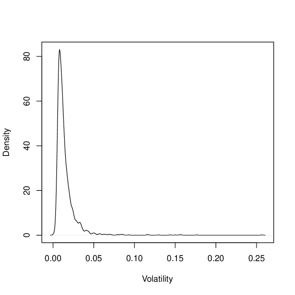
Figure 3: Density of volatility for the universe of 2000 most liquid stocks (see Section 2.6).

And the number of such stocks typically is pretty small (compared with the number of stocks in the portfolio). To illustrate this, here is an example from data. We take the data for the universe of tickers as of Sep 6, 2014 that have historical pricing data on http://finance.yahoo.com (accessed on Sep 6, 2014) for the period Aug 1, 2008 through Sep 5, 2014. We restrict this universe to include only U.S. listed common stocks and class shares (no OTCs, preferred shares, etc.) with BICS (Bloomberg Industry Classification System) sector, industry and sub-industry assignments as of Sep 6, 2014. The number of such tickers in our data is 3811. We then compute the 21-trading-day (i.e., 1-month) historical volatilities based on daily close-to-close returns for the most recent date in the data, Sep 5, 2014. One stock was not trading (zero volatility) in that 21-trading day period, so we are left with 3810 stocks with nonzero volatilities. These are our $\sigma_{i}$. The cross-sectional distribution of $\sigma_{i}$ is roughly log-normal, with a long tail at higher values (see Figures 1 and 2). The summary of these 3810 values of $\sigma_{i}$ is as follows: Min = $0.64\times 10^{-3}$, 1st Quartile = $9.16\times 10^{-3}$, Median = 0.0137, Mean = 0.0185, 3rd Quartile = 0.02197, Max = 0.3252, SD (standard deviation) = 0.01706, MAD (mean absolute deviation) = $8.37\times 10^{-3}$. Further, we have $\sigma_{*}=9.99\times 10^{-3}$, and the number of stocks in this universe with $\sigma_{i}\geq{\widetilde{\sigma}}$ is only 14. If we take 10 in the denominator instead of 5 in the definition (64), we still only get 78 stocks with $\sigma_{i}\geq{\widetilde{\sigma}}$. If we restrict our stock universe to the top 2000 most liquid stocks by ADDV (average daily dollar volume, also computed based on the same 21-trading-day period), the results are similar (also see Figures 3 and 4): Min = $0.64\times 10^{-3}$, 1st Quartile = $7.86\times 10^{-3}$, Median = 0.0111, Mean = 0.01470, 3rd Quartile = 0.01678, Max = 0.2566, SD = 0.01408, MAD = $5.60\times 10^{-3}$. Further, we have $\sigma_{*}=8.55\times 10^{-3}$, and the number of stocks in this universe with $\sigma_{i}\geq{\widetilde{\sigma}}$ is only 16. If we take 10 in the denominator instead of 5 in the definition of (64), again we still only get 69 stocks with $\sigma_{i}\geq{\widetilde{\sigma}}$.

2.7 Multifactor Risk Models

In the preceding subsection we discuss a simple 1-factor model where the pair-wise correlations (after removing the “market” mode) take two values, $\pm\rho$. (If we add back the “market” mode with a uniform correlation $\rho_{0}$, then the pair-wise correlations in the resultant correlation matrix take two values, neither of which need be (but one of them can be) negative. Our discussion above can be generalized to multifactor models (with the “market” mode removed). The math is more involved but the gist of it is captured by the 1-factor example we discuss above. Thus, we can reasonably assume that the returns $E_{i}$ are not significantly correlated with $\sigma_{i}$ or the factor loadings $\Omega_{iA}$, so that in optimizing the Fano ratio (as compared with the Sharpe ratio) the expected returns effectively get shifted by a positive additive contribution for most stocks, excepting large volatility stocks. As above, this results in fewer weights violating the bounds (13) and the portfolio is also more diversified.

3 Long-Short Portfolios

Above we discuss long-only portfolios. What about long-short portfolios? To maximize the Fano ratio, we need to maximize the objective function (11). The modulus in (11) complicates things. First, its derivative is well-defined for $w_{i}\neq 0$ and for the subset $J=\{i|w_{i}\neq 0\}$ the maximization of $g$ in (11) is equivalent to $\partial g/\partial w_{i}=0$, $i\in J$. For the sake of simplicity, let us assume that all $w_{i}\neq 0$. Then we have all the same formulas as above for the long-only portfolio (without any bounds as $w_{i}$ need no longer be nonnegative) except that $\nu_{i}$ is replaced by $\chi_{i}=\mbox{sign}(w_{i})$. So the analog of (14) now must be solved iteratively. However, here we will not delve into solving this problem (or its subtleties) as there is a more prosaic issue to address.

Ignoring the aforesaid subtleties, the equation we would need to solve iteratively reads (see (14) and the subsequent equations for definitions of $a$ and $b$)

$$w_{i}=\sum_{j=1}^{N}C^{-1}_{ij}\left[a~{}E_{j}+b~{}\chi_{j}\right]$$ (65)

where $a$ and $b$ also depend on $\chi_{i}$. However, it is not this dependence that is problematic. Instead, it is the presence of signs, i.e., $\chi_{i}$, in (65). Signs are highly unstable (they “flip-flop” a lot, especially for shorter horizons). To illustrate this, let us simplify things and consider the case of a diagonal covariance matrix $C_{ij}=\sigma_{i}^{2}~{}\delta_{ij}$. Then ${\widehat{\eta}}_{i}=E_{i}/\sigma_{i}^{2}$ and we can set $\chi_{i}=\mbox{sign}(E_{i})$. So, for a small $E_{i}$ (e.g., compared with its historical standard deviation or some suitable multiple thereof), if its sign flips (but the absolute value remains small), we can have a 100% opposite contribution from $\chi_{i}$ into (65). This is the root-cause of the aforesaid instability, which also persists even for non-diagonal $C_{ij}$ (in which case things are simply messier). We can think about this as follows. The weights (65) effectively are the same as linearly combining two strategies. One is based on optimizing the Sharpe ratio for the expected returns $E_{i}$. The other is based on optimizing the Sharpe ratio for binary expected returns $\chi_{i}=\pm 1$. It should come as no surprise to quant traders that the second strategy is suboptimal. E.g., if we take $\mbox{sign}(E_{i})$ instead of $E_{i}$ as binary expected returns, this strategy underperforms the strategy based on optimizing $E_{i}$. This is because forecasting just the direction and not the magnitude of the expected returns provides only partial information. Linearly combining such a suboptimal strategy with the strategy based on optimizing the Sharpe ratio then also is suboptimal.

Can we fix this? We can smooth out the sign in $\chi_{i}=\mbox{sign}(w_{i})$. One way to do this is to replace it by, e.g., a hyperbolic tangent: $\chi_{i}=\tanh(w_{i}/\Delta_{i})$, where $\Delta_{i}$ are some parameters. In the limit $\Delta_{i}\rightarrow 0$ we recover $\chi_{i}=\mbox{sign}(w_{i})$. Introducing $N$ new parameters $\Delta_{i}$ can be unappealing as they can easily turn out to be out-of-sample unstable. We can mitigate this, at least to a degree, by taking uniform $\Delta_{i}\equiv\Delta$ (however, we will relax this below). We then have

$$w_{i}=\sum_{j=1}^{N}C^{-1}_{ij}\left[a~{}E_{j}+b~{}\tanh(w_{j}/\Delta)\right]$$ (66)

We can solve this equation, e.g., by linearizing the hyperbolic tangent, which formally amounts to the limit where $\Delta\rightarrow\infty$, $b\rightarrow\infty$, and ${\widetilde{b}}=b/\Delta$ is kept finite:

$$w_{i}=\sum_{j=1}^{N}C^{-1}_{ij}\left[a~{}E_{j}+{\widetilde{b}}~{}w_{j}\right]$$ (67)

A formal solution reads

$$w_{i}=a\sum_{j=1}^{N}{\widetilde{C}}^{-1}_{ij}~{}E_{j}$$ (68)

$${\widetilde{C}}_{ij}=C_{ij}-{\widetilde{b}}~{}\delta_{ij}$$ (69)

The overall normalization parameter $a$ is fixed by requiring the normalization condition (2). However, the parameter ${\widetilde{b}}$ is a priori undetermined. Since we have departed from optimizing the Fano ratio, it is no longer evident what ${\widetilde{b}}$ should be. Instead of trying to fix it “theoretically”, we can take a pragmatic approach and treat ${\widetilde{b}}$ as a free parameter. For ${\widetilde{b}}=0$ we are simply optimizing the Sharpe ratio. For ${\widetilde{b}}\neq 0$, we are optimizing the Sharpe ratio but with a modified covariance matrix ${\widetilde{C}}_{ij}$, whose off-diagonal elements are the same as those of $C_{ij}$, but the diagonal elements (variances) are shifted: they can be increased (${\widetilde{b}}<0$) or decreased (${\widetilde{b}}>0$).

In this regard, it is instructive to consider the case of nonuniform $\Delta_{i}$. In this case we still have (68), where now

$${\widetilde{C}}_{ij}=C_{ij}-{\widetilde{b}}_{i}~{}\delta_{ij}$$ (70)

and ${\widetilde{b}}_{i}=b/\Delta_{i}$. Let us consider a factor model of the form (40). If we set ${\widetilde{b}}_{i}=\theta~{}\xi_{i}^{2}$, where $\xi_{i}^{2}$ are the specific variances and $\theta$ is a parameter, then for $\theta=1$ the matrix ${\widetilde{C}}_{ij}$ is singular. We can invert it in the $\theta\uparrow 1$ limit (in this limit the normalization $a$ goes to 0 such that $w_{i}$ are actually finite) and the result is that, up to an overall normalization factor (fixed via (2)), the weights $w_{i}$ are given by $\epsilon_{i}/\xi_{i}^{2}$, where $\epsilon_{i}$ are the residuals of a cross-sectional regression of $E_{i}$ over the factor loadings $\Omega_{iA}$ with the regression weights $z_{i}=1/\xi_{i}^{2}$ and no intercept [Kakushadze, 2015a]. Equivalently, ${\widetilde{\epsilon}}_{i}=\epsilon_{i}/\xi_{i}$ are the residuals of a cross-sectional regression of $E_{i}/\xi_{i}$ over the matrix $\Omega_{iA}/\xi_{i}$ with unit regression weights (and no intercept – see above). So, here we are interpolating between optimizing the Sharpe ratio and a (weighted) regression.

Formally, we can view (68) as an infinite series (here $a_{p}=a~{}{\widetilde{b}}^{p-1}$):

$$w_{i}=\sum_{p=1}^{\infty}a_{p}~{}\sum_{j=1}^{N}C^{-1}_{ij}~{}E^{(p)}_{j}$$ (71)

$$E^{(p+1)}_{i}=\sum_{j=1}^{N}C^{-1}_{ij}~{}E^{(p)}_{j}$$ (72)

$$E^{(1)}_{i}=E_{i}$$ (73)

I.e., this is a combination of “once-optimized”, “twice-optimized”, “trice-optimized”, …, strategies. In fact, we can simply forget about how we got this result (which was in an ad hoc and handwaving fashion – however, see below) and take a truncated series

$$w_{i}=\sum_{p=1}^{n_{opt}}a_{p}~{}\sum_{j=1}^{N}C^{-1}_{ij}~{}E^{(p)}_{j}=a~{}\sum_{j=1}^{N}C^{-1}_{ij}~{}{\widehat{E}}_{j}$$ (74)

where ${\widehat{E}}_{i}=\sum_{p=1}^{n_{opt}}{\widetilde{b}}^{p-1}~{}E^{(p)}_{i}$. Only one of the $n_{opt}$ coefficients $a_{p}$ is fixed by the normalization condition (2), i.e., we can fix $a_{1}=a$. As mentioned above, a priori there is no guiding principle for fixing the ${\widetilde{b}}$ parameter. However, we can require that the coefficients $a_{p}$ have the proper scaling properties under $E_{i}\rightarrow\zeta E_{i}$ and $C_{ij}\rightarrow\lambda C_{ij}$, where $\zeta>0$ and $\lambda>0$ (so that $w_{i}$ are invariant under such rescalings):

$$a_{p}\rightarrow\zeta^{-1}~{}a_{p}$$ (75)

$$a_{p}\rightarrow\lambda^{p}~{}a_{p}$$ (76)

This implies that ${\widetilde{b}}$ is invariant under $E_{i}\rightarrow\zeta E_{i}$, and we have ${\widetilde{b}}\rightarrow\lambda{\widetilde{b}}$ under $C_{ij}\rightarrow\lambda C_{ij}$. Consider ${\widetilde{b}}$ of the following form:

$${\widetilde{b}}={\widehat{b}}~{}h={\widehat{b}}~{}\sqrt{{\sum_{i,j=1}^{N}}C_{ij}^{-1}~{}E_{i}~{}E_{j}\over{\sum_{i,j=1}^{N}}C_{ij}^{-1}~{}E^{(2)}_{i}~{}E^{(2)}_{j}}$$ (77)

Then ${\widehat{b}}$ is invariant under both the $\zeta$ and $\lambda$ rescalings. We can therefore treat ${\widehat{b}}$ as a purely numerical coefficient. For instance, for $n_{opt}=2$ we have

$$w_{i}=a\left[\sum_{j=1}^{N}C^{-1}_{ij}~{}E_{j}+{\widehat{b}}~{}h~{}\sum_{j=1}^{N}C^{-1}_{ij}~{}E^{(2)}_{j}\right]$$ (78)

I.e., we are combining the “once-optimized” and “twice-optimized” strategies with the relative coefficient controlled by ${\widehat{b}}$. We discuss a backtest of this strategy below.

3.1 Bells and Whistles

While our $w_{i}$ in (74) are roughly dollar-neutral (due to the presence of the “market” mode in $C_{ij}$, which a priori need not be removed for long-short portfolios), they are not exactly dollar-neutral. We may wish our long-short portfolio to be exactly dollar-neutral (e.g., due to risk management/compliance requirements, etc.):

$$\sum_{i=1}^{N}w_{i}=0$$ (79)

More generally, we may wish to impose more than one linear homogeneous constraints

$$\sum_{i=1}^{N}G_{i\alpha}~{}w_{i}=0,~{}~{}~{}\alpha=1,\dots,m$$ (80)

where the columns of the $N\times m$ matrix $G_{i\alpha}$ are linearly independent. Such constraints are readily incorporated in the optimization problem by “padding” the factor loadings matrix with the extra $m$ columns: ${\widetilde{\Omega}}_{i{\widetilde{A}}}=(\Omega_{iA},G_{i\alpha})$, where the index ${\widetilde{A}}=(A,\alpha)\in H$ now takes ${\widetilde{K}}=|H|=K+m$ values ($H=\{{\widetilde{A}}\}$). We then have (see, e.g., [Kakushadze, 2015a])

$$C^{-1}_{ij}={1\over\xi_{i}^{2}}~{}\delta_{ij}-\sum_{{\widetilde{A}},{\widetilde{B}}\in H}{{\widetilde{\Omega}}_{i{\widetilde{A}}}\over\xi_{i}^{2}}~{}{\widetilde{Q}}^{-1}_{{\widetilde{A}}{\widetilde{B}}}~{}{{\widetilde{\Omega}}_{j{\widetilde{B}}}\over\xi_{j}^{2}}$$ (81)

$${\widetilde{Q}}_{{\widetilde{A}}{\widetilde{B}}}=\varphi_{{\widetilde{A}}{\widetilde{B}}}+\sum_{i\in J}{1\over\xi_{i}^{2}}~{}{\widetilde{\Omega}}_{i{\widetilde{A}}}~{}{\widetilde{\Omega}}_{i{\widetilde{B}}}$$ (82)

$$\varphi_{AB}=\phi_{AB}^{-1},~{}~{}~{}A,B=1,\dots,K$$ (83)

$$\varphi_{A\alpha}=0,~{}~{}~{}A=1,\dots,K,~{}\alpha=1,\dots,m$$ (84)

$$\varphi_{\alpha\beta}=0,~{}~{}~{}\alpha,\beta=1,\dots,m$$ (85)

The matrix $C^{-1}_{ij}$ has the following property:

$$\sum_{j=1}^{N}C^{-1}_{ij}~{}{\widetilde{\Omega}}_{j{\widetilde{C}}}=\sum_{{\widetilde{A}},{\widetilde{B}}\in H}{{\widetilde{\Omega}}_{i{\widetilde{A}}}\over\xi_{i}^{2}}~{}{\widetilde{Q}}^{-1}_{{\widetilde{A}}{\widetilde{B}}}~{}\varphi_{{\widetilde{B}}{\widetilde{C}}}$$ (86)

which (together with (84) and (85)) in turn implies that

$$\sum_{j=1}^{N}C^{-1}_{ij}~{}G_{j\alpha}\equiv 0,~{}~{}~{}\alpha=1,\dots,m$$ (87)

This results in a solution (74) satisfying the linear constrains (80). In practice, to minimize noise in the factor model covariance matrix, the factor loadings $\Omega_{iA}$ should be chosen orthogonal to the matrix $G_{i\alpha}$ [Kakushadze, 2015a]:

$$\sum_{i=1}^{N}\Omega_{iA}~{}G_{i\alpha}\equiv 0,~{}~{}~{}A=1,\dots,K,~{}\alpha=1,\dots,m$$ (88)

This is not required for the above “padding” trick, which works irrespective of (88).

Another consideration is that in practice one often needs to impose upper and lower bounds on $w_{i}$:

$$w_{i}^{-}\leq w_{i}\leq w_{i}^{+}$$ (89)

See [Kakushadze, 2015a] for a practically-oriented discussion. Assuming $w_{i}^{-}<0$ and $w_{i}^{+}>0$, we can readily incorporate such bounds using the algorithm given in [Kakushadze, 2015a] for which the source code is given in [Kakushadze, 2015b]. The bounds (89) are simply imposed in optimizing the Sharpe ratio with the “effective” expected returns ${\widehat{E}}_{i}$ on the r.h.s. of (74) (but no bounds are imposed in (72)).

Finally, for our backtesting purposes below, here we discuss how to include trading costs. Including nonlinear impact complicates the problem and is unnecessary for our purposes here. However, we can include linear trading costs. Below we will consider purely intraday strategies where the positions are established just once at the open and are liquidated just once at the close of the same trading day. For the stock labeled by $i$, let the linear trading cost per dollar traded be $\tau_{i}$. Then including such costs in the case of optimizing the Sharpe ratio with the expected returns $E_{i}$ amounts to replacing the expected return for the portfolio (3) by

$$E=\sum_{i=1}^{N}\left[E_{i}~{}w_{i}-\tau_{i}~{}|w_{i}|\right]$$ (90)

A complete algorithm for including linear trading cost in mean-variance optimization is given in, e.g., [Kakushadze, 2015a]. However, for our purposes here the following simple “hack” suffices. We can define the effective return

$$E_{i}^{eff}=\mbox{sign}(E_{i})~{}\mbox{max}(|E_{i}|-\tau_{i},0)$$ (91)

and simply set

$$E=\sum_{i=1}^{N}E_{i}^{eff}~{}w_{i}$$ (92)

I.e., if the magnitude for the expected return for a given stock is less than the expected cost to be incurred, we set the expected return to zero, otherwise we reduce said magnitude by said cost. This way we can avoid a nontrivial iterative procedure (see [Kakushadze, 2015a]), albeit we emphasize that this solution is only an approximation to the optimal solution. However, here we are already employing other approximations, so this way of treating linear trading costs is well-justified.

So, what should we use as $\tau_{i}$ in (91)? The model of [Almgren et al, 2005] is reasonable for our purposes here. Let $H_{i}$ be the dollar amount traded for the stock labeled by $i$. Then for the linear trading costs we have

$$T_{i}=\zeta~{}\sigma_{i}~{}{|H_{i}|\over A_{i}}$$ (93)

where $\sigma_{i}$ is the historical volatility, $A_{i}$ is the average daily dollar volume (ADDV), and $\zeta$ is an overall normalization constant we need to fix. However, above we work with weights $w_{i}$, not traded dollar amounts $H_{i}$. In our case of a purely intraday trading strategy discussed above, they are related simply via $H_{i}=I~{}w_{i}$, where $I$ is the total investment level (i.e., the total absolute dollar holdings of the portfolio after establishing it). Therefore, we have (note that $T_{i}=\tau_{i}~{}|H_{i}|=\tau_{i}~{}I~{}|w_{i}|$)

$$\tau_{i}=\zeta~{}{\sigma_{i}~{}\over A_{i}}$$ (94)

We will fix the overall normalization $\zeta$ via the following heuristic. We will (conservatively) assume that the average linear trading cost per dollar traded is 10 bps (1 bps = 1 basis point = 1/100 of 1%), i.e., $\mbox{mean}(\tau_{i})=10^{-3}$ and $\zeta=10^{-3}/\mbox{mean}(\sigma_{i}/A_{i})$.

3.2 Backtests

Here we discuss some backtests. We wish to see how “multiply-optimized” strategies (74) for dollar-neutral intraday models compare with optimizing the Sharpe ratio (i.e., a “singly-optimized” strategy). For this comparison, we run our backtests as in [Kakushadze, 2015b]. For our $C_{ij}$ (in all cases) we use heterotic risk models of [Kakushadze, 2015b]. The historical data we use in our backtests here is the same as in [Kakushadze, 2015b] and is described in detail in Subsections 6.2 and 6.3 thereof. The trading universe selection is described in Subsection 6.2 of [Kakushadze, 2015b]. We assume that the portfolio is established at the open with fills at the open prices; and ii) it is liquidated at the close on the same day – so this is a purely intraday strategy – with fills at the close prices. We include the transaction costs as discussed in Subsection 3.1 hereof. Furthermore, we include strict trading bounds (which in this case are the same as position bounds)

$$|H_{i}|\leq 0.01~{}A_{i}$$ (95)

We further impose strict dollar-neutrality on the portfolio, so that

$$\sum_{i=1}^{N}H_{i}=0$$ (96)

The total investment level in our backtests here is $I$ = $20M (i.e., $10M long and $10M short), same as in [Kakushadze, 2015b]. For the Sharpe ratio optimization with bounds we use the R function bopt.calc.opt() in Appendix C of [Kakushadze, 2015b]. We use ${\widehat{b}}=1$ (see above) in “multiply-optimized” strategies. The backtest results are summarized in Table 1, which shows that the $n_{opt}=2$ strategy outperforms the $n_{opt}=1$ strategy (which is simply optimizing the Sharpe ratio). However, for higher $n_{opt}$ it appears that we get – quite literally – “diminishing returns”.

4 Concluding Remarks

For long-only portfolios optimizing the Fano ratio effectively amounts to shifting the expected returns by a positive amount via (35), which results in fewer stocks being excluded from the portfolio due to the bounds (13) (including some stocks with negative expected returns $E_{i}$, for which effective returns ${\widetilde{E}}_{i}$ can be positive), i.e., in a more diversified portfolio (compared with optimizing the Sharpe ratio).

However, for long-short portfolios this is a non-issue to begin with: the weights need not be nonnegative. As we discuss above, optimizing the Fano ratio in this case would be suboptimal. However, the Fano ratio optimization inspires considering modifications of optimizing the Sharpe ratio, such as (66) and (67). In this regard, the following comment is in order. Linearizing the hyperbolic tangent in (66) amounts to completely removing the sign “flip-flopping” issue discussed in Section 3, which (to a lesser degree) is present even when we replace the sign in (66) by the hyperbolic tangent in (67). The further reduction via (74) essentially amounts to simply combining multiple different alphas – even though here alphas are of a specific (“multiply-optimized”) form. However, more generally, combining multiple (even a large number of) different alphas yields higher returns and Sharpe ratios and lower turnover and higher cents-per-share (see, e.g., [Kakushadze and Yu, 2017a]).

Finally, let us mention that the Fano ratio arises in the context of statistical industry classifications via clustering techniques [Kakushadze and Yu, 2016b]. One question for clustering in the context of quant trading is what to cluster? Clustering returns is suboptimal. Naively, clustering normalized returns $E_{i}/\sigma_{i}$ appears to be reasonable. However, as was argued and supported via backtests in [Kakushadze and Yu, 2016b], clustering $E_{i}/\sigma_{i}^{2}$ – i.e., the corresponding Fano ratios – is the optimal choice. Thus, clustering $E_{i}/\sigma_{i}$ groups together stocks that are (to varying degrees) highly correlated in-sample. However, there is no guarantee that they will remain as highly correlated out-of-sample. Intuitively, it is evident that higher volatility stocks are more likely to get uncorrelated with their respective clusters. This is essentially why suppressing by another factor of $\sigma_{i}$ in the Fano ratio $E_{i}/\sigma_{i}^{2}$ (as compared with $E_{i}/\sigma_{i}$) leads to better performance: inter alia, it suppresses contributions of those volatile stocks into the corresponding cluster centers [Kakushadze and Yu, 2016b].

Table 1: Simulation results for the “multiply-optimized” strategies (defined in Eq. (74) in Section 3) with bounds and costs. ROC = Return-on-Capital, SR = annualized Sharpe Ratio, CPS = cents-per-share. Note that $n_{opt}=1$ corresponds to vanilla optimization of the Sharpe ratio (i.e., a “singly-optimized” strategy).

$n_{opt}$	ROC	SR	CPS
1	35.37%	13.65	1.74
2	36.62%	15.43	2.02
3	34.00%	15.39	2.06
4	26.38%	11.80	1.69
5	17.00%	7.27	1.09

Figure 1: Density of volatility for the universe of 3810 stocks (see Section 2.6).

Figure 2: Density of log-volatility for the universe of 3810 stocks (see Section 2.6).

Figure 4: Density of log-volatility for the universe of 2000 most liquid stocks (see Section 2.6).

References

- [1]
- Adcock and Meade, 1994 Adcock, J.C. and Meade, N. (1994) A simple algorithm to incorporate transactions costs in quadratic optimization. European Journal of Operational Research 79(1): 85-94.
- Almgren et al, 2005 Almgren, R., Thum, C., Hauptmann, E. and Li, H. (2005) Equity market impact. Risk Magazine 18(7): 57-62.
- Bai, Hui and Wong, 2015 Bai, Z.D., Hui, Y.C. and Wong, W.K. (2015) Internet Bubble Examination with Mean-Variance Ratio. In: Lee, C.F. and Lee, J.C. (eds.) Handbook of Financial Econometrics and Statistics. New York, NY: Springer, pp. 1451-1465.
- Bai, Wang and Wong, 2011 Bai, Z.D., Wang, K.Y. and Wong, W.K. (2011) The mean-variance ratio test – A complement to the coefficient of variation test and the Sharpe ratio test. Statistics & Probability Letters 81(8): 1078-1085.
- Best and Hlouskova, 2003 Best, M.J. and Hlouskova, J. (2003) Portfolio selection and transactions costs. Computational Optimization and Applications 24(1): 95-116.
- Bouchaud and Potters, 2011 Bouchaud, J.-P. and Potters, M. (2011) Financial applications of random matrix theory: a short review. In: Akemann, G., Baik, J. and Di Francesco, P. (eds.) The Oxford Handbook of Random Matrix Theory. Oxford, United Kingdom: Oxford University Press.
- Bowler and Wentz, 2005 Bowler, B. and Wentz, P. (2005) Portfolio Optimization: MAD vs. Markowitz. Undergraduate Math Journal (Rose-Hulman Instritute of Technology) 6(2): 3.
- Braga, 2016 Braga M.D. (2016) Alternative Approaches to Traditional Mean-Variance Optimisation. In: Basile, I. and Ferrari, P. (eds) Asset Management and Institutional Investors. Cham, Switzerland: Springer, pp. 203-213.
- Cadenillas and Pliska, 1999 Cadenillas, A. and Pliska, S.R. (1999) Optimal trading of a security when there are taxes and transaction costs. Finance and Stochastics 3(2): 137-165.
- Delbos and Gilbert, 2005 Delbos, F. and Gilbert, J.C. (2005) Global linear convergence of an augmented Lagrangian algorithm for solving convex quadratic optimization problems. Journal of Convex Analysis 12(1): 45-69.
- den Hertog, 1992 den Hertog, D. (1992) Interior Point Approach to Linear, Quadratic and Convex Programming. Mathematics and its Applications 277. Dordrecht, The Netherlands: Kluwer Academic Publishers.
- Fano, 1947 Fano, U. (1947) Ionization Yield of Radiations. II. The Fluctuations of the Number of Ions. Physical Review 72(1): 26.
- Grinold and Kahn, 2000 Grinold, R.C. and Kahn, R.N. (2000) Active Portfolio Management. New York, NY: McGraw-Hill.
- Janeček and Shreve, 2004 Janeček, K. and Shreve, S. (2004) Asymptotic analysis for optimal investment and consumption with transaction costs. Finance and Stochastics 8(2): 181-206.
- Jansen, 1997 Jansen, B. (1997) Interior Point Techniques in Optimization – Complementarity, Sensitivity and Algorithms. Applied Optimization 6. Dordrecht, The Netherlands: Kluwer Academic Publishers.
-
Kakushadze, 2015a
Kakushadze, Z. (2015a)
Mean-Reversion and Optimization.
Journal of Asset Management 16(1): 14-40.
Available online: http://ssrn.com/abstract=2478345. - Kakushadze, 2015b Kakushadze, Z. (2015b) Heterotic Risk Models. Wilmott Magazine 2015(80): 40-55. Available online: http://ssrn.com/abstract=2600798.
- Kakushadze, 2016 Kakushadze, Z. (2016) 101 Formulaic Alphas. Wilmott Magazine 2016(84): 72-80. Available online: http://ssrn.com/abstract=2701346.
- Kakushadze, 2017 Kakushadze, Z. (2017) On Origins of Bubbles. Journal of Risk & Control 4(1): 1-30. Available online: http://ssrn.com/abstract=2830773.
-
Kakushadze and Yu, 2016a
Kakushadze, Z. and Yu, W. (2016a)
Multifactor Risk Models and Heterotic CAPM.
The Journal of Investment Strategies 5(4): 1-49.
Available online: http://ssrn.com/abstract=2722093. -
Kakushadze and Yu, 2016b
Kakushadze, Z. and Yu, W. (2016b)
Statistical Industry Classification.
Journal of Risk & Control 3(1) (2016) 17-65.
Available online: http://ssrn.com/abstract=2802753. -
Kakushadze and Yu, 2017a
Kakushadze, Z. and Yu, W. (2017a)
How to Combine a Billion Alphas.
Journal of Asset Management 18(1): 64-80.
Available online: http://ssrn.com/abstract=2739219. -
Kakushadze and Yu, 2017b
Kakushadze, Z. and Yu, W. (2017b)
Statistical Risk Models.
The Journal of Investment Strategies 6(2): 1-40.
Available online: http://ssrn.com/abstract=2732453. - Kellerer, Mansini and Speranza, 2000 Kellerer, H., Mansini, R. and Speranza, M.G. (2000) Selecting Portfolios with Fixed Costs and Minimum Transaction Lots. Annals of Operations Research, 99(1-4): 287-304.
- Konno and Yamazaki, 1991 Konno, H. and Yamazaki, H. (1991) Mean-Absolute Deviation Portfolio Optimization Model and Its Applications to Tokyo Stock Market. Management Science 37(5): 519-531.
- Lo and Patel 2008 Lo, A.W. and Patel, P.N. (2008) 130/30: The New Long-Only. The Journal of Portfolio Management 34(2): 12-38.
- Lobo, Fazel and Boyd, 2007 Lobo, M.S., Fazel, M. and Boyd, S. (2007) Portfolio optimization with linear and fixed transaction costs. Annals of Opererations Research 152(1): 341-365.
- Markowitz, 1952 Markowitz, H. (1952) Portfolio selection. The Journal of Finance 7(1): 77-91.
- Michaud and Michaud, 2008 Michaud, R. and Michaud, R. (2008) Efficient Asset Management: A practical Guide to Stock Portfolio Optimization and Asset Allocation. (2nd ed.) Oxford, UK: Oxford University Press.
- Mokkhavesa and Atkinson, 2002 Mokkhavesa, S. and Atkinson, C. (2002) Perturbation solution of optimal portfolio theory with transaction costs for any utility function. IMA Journal of Management Mathematics 13(2): 131-151.
- Murty, 1988 Murty, K.G. (1988) Linear Complementarity, Linear and Non-linear Programming. Sigma Series in Applied Mathematics 3. Berlin: Heldermann Verlag.
- Pang, 1983 Pang, J.-S. (1983) Methods for quadratic programming: A survey. Computers & Chemical Engineering 7(5): 583-594.
- Patel and Subrahmanyam, 1982 Patel, N.R. and Subrahmanyam, M.G. (1982). A Simple Algorithm for Optimal Portfolio Selection with Fixed Transaction Costs. Management Science 28(3): 303-314.
- Rockafellar and Uryasev, 2000 Rockafellar, R.T. and Uryasev, S. (2000) Optimization of Conditional Value-At-Risk. The Journal of Risk 2(3): 21-41.
- Roy and Vetterli, 2007 Roy, O. and Vetterli, M. (2007) The effective rank: A measure of effective dimensionality. In: Proceedings – EUSIPCO 2007, 15th European Signal Processing Conference. Poznań, Poland (September 3-7), pp. 606-610.
- Sharpe, 1966 Sharpe, W.F. (1966) Mutual Fund Performance. Journal of Business 39(1): 119-138.
- Sharpe, 1994 Sharpe, W.F. (1994) The Sharpe Ratio. The Journal of Portfolio Management 21(1): 49-58.
- Shreve and Soner, 1994 Shreve, S. and Soner, H.M. (1994) Optimal investment and consumption with transaction costs. The Annals of Applied Probability 4(3): 609-692.