Useq Ucyc Xxx Yyy Zzz Www

Split-Decomposition Trees with Prime Nodes:
Enumeration and Random Generation of Cactus Graphs

Abstract

In this paper, we build on recent results by Chauve et al. and Bahrani and Lumbroso, which combined the split-decomposition, as exposed by Gioan and Paul, with analytic combinatorics, to produce new enumerative results on graphs—in particular the enumeration of several subclasses of perfect graphs (distance-hereditary, 3-leaf power, ptolemaic).

Our goal was to study a simple family of graphs, of which the split-decomposition trees have prime nodes drawn from an enumerable (and manageable!) set of graphs. Cactus graphs, which we describe in more detail further down in this paper, can be thought of as trees with their edges replaced by cycles (of arbitrary lengths). Their split-decomposition trees contain prime nodes that are cycles, making them ideal to study.

We derive a characterization for the split-decomposition trees of cactus graphs, produce a general template of symbolic grammars for cactus graphs, and implement random generation for these graphs, building on work by Iriza.

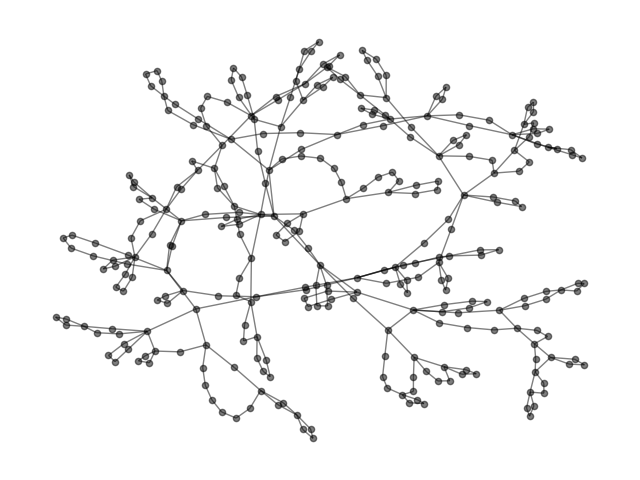
(a) A random mixed cactus graph with 309 vertices and 80 cycles.

(b) A random mixed cactus graph with 933 vertices and 239 cycles.

Figure 1: Our symbolic grammars can be used to create Boltzmann samplers for the uniform random generation of large cactus graphs. Here we have included two cactus graphs, each of which has been drawn uniformly at random from the family of unlabeled, plane, rooted cacti where each cycle has at least 4 nodes.

Introduction

LimeGreenTODO Jérémie: Write segue for split-decomposition using tree decompositions.

In general, counting graphs is much more difficult than counting trees—the latter are completely recursive, and as such, there are many generic results and theorems that can be applied straightforwardly [FlSe09]. Graphs, on the other hand, can have cycles and can thus not be specified recursively in the general case. A tree decomposition is a method by which graphs are put in correspondence with rooted trees (usually bijectively), which are easier to specify and study; to convert a graph to a tree, the decomposition makes certain hypotheses on the structure of the graphs.

There exists a number of tree decompositions, and several have been used in the context of analytic combinatorics. Most recently, Chauve et al. [ChFuLu17] have used the split decomposition to provide the first exact enumeration of distance-hereditary graphs (the largest subset of graphs that can be entirely decomposed with the split-decomposition).

The split decomposition and prime nodes.

Informally, a split in a graph is a bipartition of the vertices into two sets of size at least 2, such that the edges between the sets form a complete bipartite graph. All splits of a graph form a tree-like structure, where each internal node of the tree is labeled with a graph. The split decomposition [GiPa12] refers to the process of transforming a graph into a graph-labeled tree using splits of the original graph.

The split decomposition was first introduced by Cunningham [Cunningham82] and later reformulated by Gioan and Paul [GiPa12], who introduced the concept of graph-labeled trees. More recently, Chauve et al. [ChFuLu14, ChFuLu17] observed that these graph-labeled trees are well-suited for recursive symbolic specification, which they used to provide, among other things, the first exact enumeration of distance-hereditary graphs. Distance-hereditary graphs are the totally decomposable graphs for the split decomposition [GiPa12, Cunningham82], and therefore a natural first class of graphs to study when considering the split decomposition for enumerating graphs.

The paper by Chauve et al. [ChFuLu17] was first in a line of work on the application of the split decomposition to graph enumeration. Bahrani and Lumbroso [BaLu17] used the same framework to give grammars for subsets of distance-hereditary graphs that are specified in terms of forbidden induced subgraphs. They showed that constraining a split decomposition tree to avoid certain patterns can help avoid corresponding induced subgraphs in the original graph. The ability to forbid induced subgraphs led to grammars and full enumeration for a wide set of graph classes: ptolemaic, block, and variants of cactus graphs (2,3-cacti, 3-cacti and 4-cacti). In certain cases, no enumeration was known (ptolemaic, 4-cacti); in other cases, although the enumerations were known, an abundant potential is unlocked by the provided grammars (in terms of asymptotic analysis, random generation, and parameter analysis, etc.).

The methodology has shown its potential in this line of work, specially in providing grammars for totally decomposable graph classes, i.e. distance-hereditary graphs and their subfamilies. As stated by Bahrani and Lumbroso [BaLu17], the natural next step to develop its reach is to study split decomposition trees that are not fully decomposable and contain prime nodes. This is part of the motivation behind studying cactus graphs, which result in split decomposition trees with prime polygonal nodes. As such, this paper is the first work in the line of papers introduced above to examine split decomposition trees that are not fully decomposable.

Cactus graphs.

A cactus is a graph in which no two cycles share an edge. It can be thought of as a collection of polygons and bridges that pairwise share at most one vertex. Cactus graphs come in many flavors (e.g. see Figure 2):

• A cactus graph is pure if all its cycles have the same size; it is mixed otherwise.

• A graph is labeled if its vertices are distinguished for the purpose of enumeration; it is unlabeled if the vertices have no distinct identification besides their adjacencies.

• A rooted graph has one distinguished vertex; it is otherwise called unrooted.

• A plane cactus graph is embedded in the plane so that every vertex is paired with a circular permutation of the edges incident to it; when this permutation is insignificant, the cactus graph is called non-plane or free.

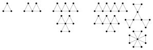
Figure 2: Small (unrooted, unlabeled, pure, free) 3-cacti

Besides being objects of interest in combinatorics, cactus graphs have applications in other fields. For example, many hard problems on general graphs have efficient algorithms on cactus graphs [baste2017parameterized, chandran2017algorithms, das2014cactus]. Cactus graphs are also used in modeling electronic circuits [nishi1984topological], networks [arcak2011diagonal], and comparative genomics [paten2011cactus].

The problem of enumerating cactus graphs was first proposed in 1950 in a lecture by Uhlenbeck [UhlenbeckLecture], where these graphs were referred to as Husimi Trees. Subsequently, Harry and Uhlenbeck [HaUh53] as well as Ford and coauthors [ford1956combinatorialI, ford1956combinatorialII, ford1956combinatorialIII, ford1957combinatorialIV] and Bergeron et al. [bergeron1998combinatorial] have examined the enumeration of unlabeled and labeled cactus graphs in a series of notes. These works derive functional equations for the generating functions of cactus graphs, with no convenient way of obtaining a few hundred terms of the enumeration or the prospect of building random generators. Additionally, their methodology is dependent upon the symmetric structure of cycles in cactus graphs and therefore hard to generalize to other graph classes. More recently, Bona et al. [bona2000enumeration] derived the enumeration of plane cactus graphs, but their methodology does not seem to generalize to non-plane cacti.

The goal of this paper is to develop a simple, extendable framework that not only allows for enumerating all aforementioned varieties of cactus graphs but also is amenable to imposing arbitrary restrictions on the structure of the graphs as well as random generation. This goal is achieved by developing symbolic grammars for different varieties of cactus graphs.

Since cactus graphs are very similar to trees, the same grammars can be developed more directly by exploiting this apparent recursivity. However, while the entire machinery introduced in this paper is not necessary to obtain grammars for cactus graphs, these tools belong to a more general and powerful framework developed by Chauve et al. [ChFuLu17] and extended by Bahrani and Lumbroso [BaLu17]. This framework is highly flexible and can be generalized to obtain grammars for many other classes of cactus graphs. We therefore believe it is informative to state our results within this framework, specially since our original investigation was to look at identifying characterizable families of graphs of which the split decomposition trees contain a manageable family of prime nodes (in this case: various cycles and sequences).

1 Definitions and preliminaries

In this section, we introduce standard definitions from graph theory (1.1), followed by a formal introduction to the split-decomposition expressed in terms of graph-labeled trees (1.2 and 1.3), which are the tools also used by Chauve et al. [ChFuLu17] and Bahrani and Lumbroso [BaLu17].

1.1 Graph definitions.

For a graph $G$, we denote by $V(G)$ its vertex set and $E(G)$ its edge set.

Moreover, for a vertex $x$ of a graph $G$, we denote by $N(x)$ the neighborhood of $x$, that is the set of vertices $y$ such that $\{x,y\}\in E(G)$; this notion extends naturally to vertex sets: if $\cramped{V_{1}}\subseteq V(G)$, then $N(\cramped{V_{1}})$ is the set of vertices defined by the (non-disjoint) union of the neighborhoods of the vertices in $\cramped{V_{1}}$. The subgraph of $G$ induced by a subset $\cramped{V_{1}}$ of vertices is denoted by $G[\cramped{V_{1}}]$.

A clique on $k$ vertices, denoted by $\cramped{K_{k}}$, is the complete graph on $k$ vertices (i.e., there exists an edge between every pair of vertices). A star on $k$ vertices, denoted by $\cramped{S_{k}}$, is the graph with one vertex of degree $k-1$ (the center of the star) and $k-1$ vertices of degree $1$ (the extremities of the star).

A closed walk in a graph is an alternating sequence of vertices and edges, starting and ending at the same vertex, where each edge is adjacent in the sequence to its endpoints. A cycle is a closed walk in which no repetitions of vertices and edges are allowed, except for the starting and ending point. We use the terms cycles and polygons interchangeably. In this paper we work with simple graphs (i.e. graphs without self-loops or multi-edges), so all cycles have at least 3 distinct vertices.

1.2 Graph-labeled trees.

We first introduce the notion of graph-labeled tree, due to Gioan and Paul [GiPa12], then define the split-decomposition and finally give the characterization of a reduced split-decomposition tree, described as a graph-labeled tree.

Definition 1.1.

A graph-labeled tree $(T,\cls{F})$ is a tree $T$ in which every internal node $v$ of degree $k$ is labeled by a graph $\cramped{G_{v}}\in\cls{F}$ on $k$ vertices, called marker vertices, such that there is a bijection $\cramped{\rho_{v}}$ between the edges of $T$ incident to $v$ and the vertices of $\cramped{G_{v}}$.

For example, in Figure 3 the internal nodes of $T$ are denoted by large circles, the marker vertices are denoted by small hollow circles, the leaves of $T$ are denoted by small solid circles, and the bijection $\cramped{\rho_{v}}$ is denoted by each edge that crosses the boundary of an internal node and ends at a marker vertex.

These graph-labeled trees are a powerful tool for studying the structure of the original graph they describe. Some elements of the terminology have been summarized in Figure 4 (reproduced from Bahrani and Lumbroso [BaLu17]), as they are frequently referenced in the proofs of Section 2.

Definition 1.2.

Let $(T,\cls{F})$ be a graph-labeled tree and let $\ell,\ell^{\prime}\in V(T)$ be leaves of $T$. We say that there is an alternated path between $\ell$ and $\ell^{\prime}$, if there exists a path from $\ell$ to $\ell^{\prime}$ in $T$ such that for any adjacent edges $e=\set{u,v}$ and $e^{\prime}=\set{v,w}$ on the path, $\set{\cramped{\rho_{v}}(e),\cramped{\rho_{v}}(e^{\prime})}\in E(\cramped{G_{v}})$.

Definition 1.3.

The original graph, also called accessibility graph, of a graph-labeled tree $(T,\cls{F})$ is the graph $G$ where $V(G)$ is the leaf set of $T$ and, for $x,y\in V(G)$, $\set{x,y}\in E(G)$ iff there is an alternated path between $x$ and $y$ in $T$.

Figures 3 and 4 (reproduced from Bahrani and Lumbroso [BaLu17]) illustrate the concept of an alternated path: it is, more informally, a path that only ever uses at most one interior edge of any graph label.

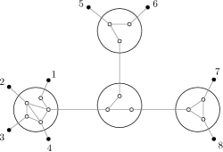
(a) A graph-labeled tree.

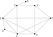
(b) Original graph for (or accessibility graph of) the graph-labeled tree in Figure 3.

Figure 3: Two leaves of the split-decomposition graph-labeled tree (left) correspond to adjacent vertices in the original graph that was decomposed (right) if there exists an alternated path: a path between those leaves, which uses at most one interior edge of any graph label. For example, vertex 5 is adjacent to vertex 4 in the original graph, because there is an alternated path between the two corresponding leaves in the split-decomposition tree; vertex 5 is not adjacent to vertex 3 however, because that would require the path to take two interior edges of the (prime) leftmost graph-label.

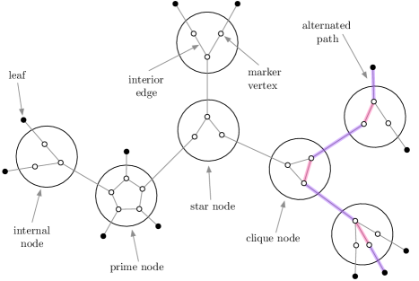
Figure 4: In this figure, we present a few terms that we use a lot in this article.

1.3 Split-decomposition.

In this section we summarize various concepts, a more formal and comprehensive treatment of which can be found in previous work [ChFuLu17, BaLu17].

A split in a graph is a bipartition of the vertices into two sets of size at least 2, such that the edges between the two sets form a complete bipartite graph. More formally,

Definition 1.4.

A split [Cunningham82] of a graph $G$ with vertex set $V$ is a bipartition $(\cramped{V_{1}},\cramped{V_{2}})$ of $V$ (i.e., $V=\cramped{V_{1}}\cup V_{2}$, $\cramped{V_{1}}\cap\cramped{V_{2}}=\emptyset$) such that

1. $|V_{1}|\geqslant 2$ and $|V_{2}|\geqslant 2$;

2. every vertex of $N(\cramped{V_{1}})$ is adjacent to every vertex of $N(\cramped{V_{2}})$.

A graph without any split is called a prime graph. A graph is degenerate if any bipartition of its vertices into sets of size at least 2 is a split: cliques and stars are the only such graphs.

Informally, the split-decomposition of a graph $G$ consists of finding a split $(\cramped{V_{1}},\cramped{V_{2}})$ in $G$, followed by decomposing $G$ into two graphs $\cramped{G_{1}}=G[\cramped{V_{1}}\cup\{\cramped{x_{1}}\}]$, where $\cramped{x_{1}}\in N(\cramped{V_{1}})$, and $\cramped{G_{2}}=G[\cramped{V_{2}}\cup\{\cramped{x_{2}}\}]$, where $\cramped{x_{2}}\in N(\cramped{V_{2}})$, and then recursively decomposing $\cramped{G_{1}}$ and $\cramped{G_{2}}$. This decomposition naturally defines an unrooted tree structure, called a split-decomposition tree, in which the internal vertices are labeled by degenerate or prime graphs and the leaves are in bijection with $V(G)$.

The structure of the split decomposition tree of a graph may depend on the specific sequence of split operations performed on it. However, Cunningham [Cunningham82] provided a set of criteria that are satisfied by exactly one split decomposition tree for every graph. This uniqueness result is reformulated below in terms of graph-labeled trees by Gioan and Paul [GiPa12]. [Cunningham [Cunningham82]]For every connected graph $G$, there exists a unique split-decomposition tree such that:

1. every non-leaf node has degree at least three;

2. no tree edge links two vertices with clique labels;

3. no tree edge links the center of a star to the extremity of another star.

Such a tree is called reduced, and this theorem establishes a bijection between graphs and their reduced split decomposition trees.

2 Split-Decomposition of cactus graphs

In this section, we first introduce a bijective split decomposition tree characterization of general cactus graphs. We then make certain simplifications to that characterization, which, while respecting its bijective nature, make its correspondence with our cactus grammars more apparent. Additionally, these characterizations make apparent how arbitrary size constraints on cycles of a cactus graph translate into modifications in its split-decomposition tree characterization, which can then be directly translated into modifications in the grammar.

First, we provide a characterization for the reduced split decomposition trees of general cactus graphs. The following lemma will be used in the proof of Theorem 2.3.

Lemma 2.1 (Polygon primality).

Polygons of size at least 5 are prime with respect to the split decomposition.

Proof 2.2.

We will show that a cycle with at least 5 vertices has no splits. Suppose, on the contrary, that such a split exists.

We claim that there are at least two disjoint edges crossing the split. Any bipartition of a cycle has at least two edges crossing it. Suppose all edges crossing the bipartition are non-disjoint. Then they must all be incident to the same vertex $v$ in one side of the split. Since the degree of every vertex in a cycle is 2, there must be exactly two edges crossing the split, both of which are incident to $v$. This implies that $v$ is the only vertex in its side of the split: Any other vertex on the same side cannot have a path to $v$ without either crossing the split or causing $v$ to have degree higher than 2. Since a cycle is connected to begin with, no other vertex besides $v$ can belong to the same side of the split. This contradicts the requirement that each side of a split must have at least 2 vertices.

Let $\{x,u\}$ and $\{y,v\}$ be two disjoint edges crossing a split in a cycle with at least 5 vertices (with $x$ and $y$ on one side of the split and $u$ and $v$ on the other side). Since the edges crossing a split must induce a complete bipartite graph, the edges $\{x,v\}$ and $\{y,u\}$ must also be present in the graph. Therefore, the graph must have a cycle of size 4 as a subgraph, which is not the case for any cycle with at least 5 vertices.

Theorem 2.3 (Reduced split tree characterization of general cactus graphs).

A graph $G$ with the reduced split decomposition tree $(T,\mathcal{F})$ is a cactus graph if and only if

1. $\mathcal{F}$ consists of stars and polygons of size 3 or at least 5;

2. the center of every star-node in $T$ is attached to either

   1. a leaf, or

   2. the center of another star-node, only as long as both star-nodes have exactly two extremities;

3. every extremity of star-nodes in $T$ is attached to either

   1. a polygon,

   2. a leaf, or

   3. an extremity of another star-node;

4. no two polygons are adjacent.

Proof 2.4.

[$\Rightarrow$]  Let $G$ be a cactus graph with the corresponding reduced split decomposition tree $T$. We will show that $T$ satisfies all the conditions of the theorem.

A block in a graph is a maximal 2-connected subgraph, or a subgraph formed by a bridge or an isolated vertex. In the case of a cactus graph, a block is either a cycle, or an edge that does not belong to any cycles. Let a cluster in a cactus graph be a maximal set of at least two blocks, all of which share exactly one vertex.

Furthermore, we define external blocks and clusters in cactus graphs in a similar way to external nodes in trees. A block in a cactus graph is called external if it shares exactly one vertex with other blocks. A cluster is external if it contains an external block. Note that this analogy captures the underlying tree structure for every cactus graph, where every cluster is a node in the tree, and two clusters share an edge iff they share a block. It is easy to see that the resulting graph is indeed connected and acyclic, with external clusters of the cactus graph corresponding to external nodes in the underlying tree. These definitions are illustrated in Figure 5.

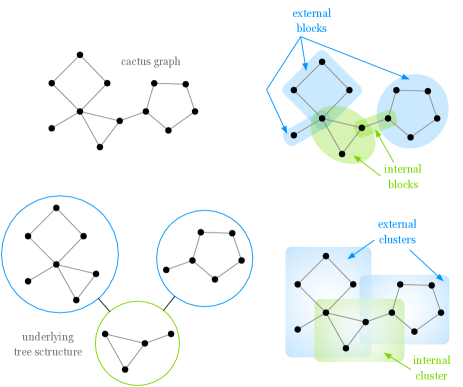
Figure 5: This figure illustrates the terminology introduced as part of the proof of Theorem 2.3. The top left graph is a cactus graph. The top right figure highlights all the blocks of this cactus graph, and the bottom right figure shows all its clusters. The bottom left figure shows the underlying tree structure of this cactus graph, where each node corresponds to a cluster and each edge represents a pair of clusters sharing a block. In all these figures, blue denotes external units (i.e. blocks, clusters, underlying tree nodes) whereas green indicates internal units.

We will proceed by induction on the number of clusters in $G$. For the base case, we consider cactus graphs with zero clusters. In this case, the graph consists of exactly one block, which can be one of the following (also shown in Figure 6):

• an edge: In this case, the corresponding reduced split decomposition tree is just an edge.

• a cycle of size 3 or at least 5: In this case, the corresponding reduced split decomposition tree is an internal node labeled with a cycle of the same size as the block, with a leaf hanging from every vertex of the label. 

• a cycle of size 4: In this case, the corresponding reduced split decomposition tree is two internal nodes, each labeled with a star with two extremities. The centers of the stars are connected by an edge, and the extremities of the stars are connected to leaves.

It is easy to confirm that the split decomposition trees above are both correct (by making sure their alternated paths match the adjacencies of the corresponding cluster) and reduced (by making sure the conditions of Theorem 1.4 are met). Furthermore, all the above split decomposition trees satisfy the conditions of this theorem, thus proving our base case.

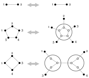
Figure 6: This figure shows the base case in part of the proof of Theorem 2.3, i.e. split decomposition trees of cactus graphs with exactly one block (and thus zero clusters). These graphs are partitioned into three disjoint subsets: an edge, a cycle of size 3 or at least 5, and a cycle of size 4. Each subset is treated differently as illustrated above. Note that the numbers here serve to specify the bijection between the vertices of each cactus graph and the leaves of its split decomposition tree. They do not serve to distinguish the vertices and do not imply that these graphs are labeled.

For the inductive step, let $G$ be a cactus graph with at least one cluster. First, we claim that $G$ must have an external cluster, since the underlying tree must have a leaf. Let $C$ be an external cluster including blocks $\cramped{S_{1}}\cdots\cramped{S_{k}},k>1$, all of which share the vertex $v\in V(G)$. Finally, observe that at most one of the blocks is internal (the block representing the edge between the node corresponding to $C$ and its neighbor in the underlying tree is internal). Without loss of generality, assume that $\cramped{S_{k}}$ is the internal block, if one exists.

We split the cluster $C$ from the rest of the cactus graph and create a graph-labeled tree $\tilde{T}$ as follows (Figure 7):

• Create a star-node $s$ with $k$ extremities, one per block, respecting the blocks’ circular permutation around $v$ in the case of plane cacti. Attach the center of this star-node to a leaf corresponding to $v$.

• For every external block $\cramped{S_{i}},i<k$,

  • If $\cramped{S_{i}}$ is a single edge, attach its corresponding extremity to a leaf.

  • If $S_{i}$ is a cycle of size 4, create two star-nodes with two extremities each, where the pair of extremities of each star represent two non-adjacent vertices in $\cramped{S_{i}}$, with the order of the appearance of the extremities respecting the planar embedding of the corresponding vertices in the case of plane cacti. Attach the two stars together at their centers, and connect the extremity corresponding to $v$ with the extremity of $s$ corresponding to $\cramped{S_{i}}$, and connect the other three extremities to leaves.

  • Otherwise, create an internal node labeled with $\cramped{S_{i}}$. Attach the copy of $v$ in the label of the new internal node to the extremity of $s$ corresponding to $\cramped{S_{i}}$. Attach every other vertex in the label of the new internal node to a leaf, representing the vertices of $G$ in $\cramped{S_{i}}$, respecting their planar ordering.

• Next, consider $G^{\prime}$, the remainder of $G$ excluding the external blocks $\cramped{S_{i}},i<k$ but including $\cramped{S_{k}}$. This is a cactus graph with fewer clusters than $G$. Applying the inductive hypothesis, we obtain a reduced split-decomposition tree $\tilde{T}^{\prime}$ satisfying the conditions of this theorem. Finally, we attach $\tilde{T}^{\prime}$ to $s$ by removing the leaf corresponding to $v$ in $V(\tilde{T}^{\prime})$ and connecting the edge incident to that leaf with the extremity of $s$ corresponding to $\cramped{S_{k}}$.

Note that this procedure produces a split-decomposition tree $\tilde{T}$ that satisfies the conditions of this theorem. In every step, the new star-node and the nodes corresponding to external blocks satisfy the conditions by construction, and the nodes within $G^{\prime}$ satisfy the conditions by the inductive hypothesis. It remains to check that nothing is violated upon attaching $\tilde{T}^{\prime}$ to an extremity of the new star-node. Since $v$ belongs to a single external block in $G^{\prime}$, its corresponding leaf in $\tilde{T}^{\prime}$ can only be attached to either a star extremity or a polygon; this is because the only time a leaf is attached to a star center is when the leaf corresponded to the common vertex of a cluster in the inductive step, in which case it was shared between more than one block. Therefore, only conditions 3 and 4 are relevant, both of which are satisfied when attaching the extremity of $s$ to $v$’s neighbor in $\tilde{T}^{\prime}$.

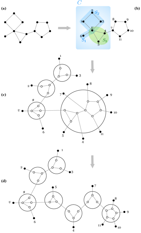
Figure 7: This figure shows the inductive step used in the proof of Theorem 2.3, i.e.. The inductive step begins by identifying an external cluster $C$, which consists of blocks $\cramped{S_{1}}\cdots\cramped{S_{k}}$, all of which share a vertex $v$. The external blocks (here $\cramped{S_{1}}$ and $\cramped{S_{2}}$) are then separated via a star node $s$, the center of which is attached to $v$. The rest of the cactus graph forms a large super node hanging from $s$, and will be decomposed using the inductive hypothesis. Furthermore, the specific plane embedding of the original cactus graph around $v$ can be respected by the choice of the order of the extremities of $s$. Similar to Figure 6, the numbers here are merely for illustrative purposes and do not imply that the cactus graph is labeled.

Finally, we need to show that this procedure preserves the adjacencies of $G$.

First, we show that every step in the procedure above preserves the adjacencies of $G$ via alternated paths in $\tilde{T}$. At every step, any edge $e=\{x,y\}\in E(G)$ must belong to one of the following cases.

• $e$ is incident to $v$: In this case, $e$ must belong to a block $\cramped{S_{i}},i\leqslant k$. There is an alternated path from $v$ to the center of the star-node attached to $v$, then to the extremity corresponding to $\cramped{S_{i}}$ and then out of the star-node. From there,

  • if $\cramped{S_{i}}$ is an edge, we arrive at a leaf representing the other end of $e$, completing our alternated path;

  • if $\cramped{S_{i}}$ is an external cycle of size 4, we next arrive at the extremity of a star-node and can continue to its center, then to the center of the neighboring star-node, then to the extremity of the current star-node corresponding to the other end of $e$, and finally to the leaf corresponding to the other end of $e$;

  • finally, if $\cramped{S_{i}}$ is an external cycle of size 3 or at least 5 or an internal cycle, we next arrive at an internal node labeled with either $\cramped{S_{i}}$ or $G^{\prime}$, both of which include $e$ as an edge within the label. We can therefore continue the alternated path by taking the edge corresponding to $e$ from within the label and then to the leaf corresponding to the other end of $e$.

• $e$ is not incident to $v$: In this case, $e$ belongs to either $\cramped{S_{i}},i<k$ or $G^{\prime}$. Note that in the first case $\cramped{S_{i}}$ cannot be an edge since $v\not\in e$.

  • If $\cramped{S_{i}}$ is a cycle of size 4, there is an alternated path representing $e$ starting from the leaf corresponding to $x$ to an extremity of the neighboring star, then to its center, then to the center of the next star, and finally to the extremity of the same star corresponding to the leaf $y$ and lastly to the leaf corresponding to $y$ itself.

  • Otherwise, $\cramped{S_{i}}$ is either cycle of size 3 or at least 5, or $G^{\prime}$. In all these cases, $e$ is present as within the label of an internal node, and thus there is an alternated path between the leaves representing $x$ and $y$ that takes that edge within a graph label corresponding to $e$.

Therefore, at every step, including the base case, for every edge in $G$ there exists an alternated path in $\tilde{T}$.

In the other direction, we have to show that in every step, for every alternated path in $\tilde{T}$ there is an edge in $G$. Take a pair of vertices $x,y\in V(G),\{x,y\}\not\in E(G)$. It is easy to check that if $x$ and $y$ belong to the same block $\cramped{S_{i}}$ of size at least 5, any path between the leaves representing them in $\tilde{T}$ uses more than one edge from the the internal node labeled with $\cramped{S_{i}}$. Furthermore, if $x$ and $y$ belong to the same block of size 4 or different blocks, any path connected the leaves representing them uses two edges from the same star-node.

Finally, note that the conditions of this theorem imply that $T$ is reduced: Cunningham’s theorem’s (Section 1.4) criterion 1 for being reduced is satisfied by condition 1 of this theorem, criterion 2 by condition 4 of this theorem, and criterion 3 by conditions 2 and 3 of this theorem. Therefore, the procedure above produces a reduced split-decomposition tree, which is guaranteed to be unique by Cunningham’s theorem. Thus, $\tilde{T}$ and $T$ are the same split-decomposition tree.

Therefore, the adjacencies of $G$ correspond bijectively to the alternated paths of $T$. Furthermore, the plane embedding of a cactus graph can be preserved if the cyclic order of the new star-node in every step respects the plane embedding of the corresponding blocks in $G$.

[$\Leftarrow$]  Let $T$ be a reduced split-decomposition tree satisfying the conditions of this theorem. We should show that the original graph corresponding to $T$ is indeed a cactus.

In the first part of the proof, we introduced a procedure for constructing the reduced split-decomposition tree of any cactus graph. The reverse of the same procedure can be used to build the original cactus graph from a split-decomposition tree. More specifically, pairs of star-nodes connected via their centers can be combined to form cycles of size 4, and star-nodes with a leaf hanging from their center can be combined with their neighbors in the reverse direction of the procedure as well. It is easy to check that as long as $T$ has more than one internal node, it is possible to combine some internal nodes into one. Furthermore, these reverse steps maintain the invariant that in all intermediate split-decomposition trees, all the created labels are cactus graphs. Therefore, at the end of this procedure, a split decomposition tree with a single internal node remains, the label of which must also be a cactus graph.

Theorem 2.3 gives a bijective characterization of cactus graphs in terms of reduced split-decomposition trees. In its proof we utilize Cunningham’s Theorem, which guarantees uniqueness of the reduced split-decomposition tree for any graph. It turns out, however, that the characterization for general cactus graphs can be simplified to the form in Theorem 2.5, using a bijection between the reduced split-decomposition trees in Theorem 2.3 and a simpler, yet not reduced, set of split-decomposition trees.

Theorem 2.5 (Split tree characterization of general cactus graphs).

Cactus graphs are in bijection with split-decomposition trees where

1. internal nodes are stars and polygons;

2. the centers of all star-nodes are attached to leaves;

3. the extremities of star-nodes are attached to leaves or polygons.

Proof 2.6.

Since the characterization in Theorem 2.3 describes a reduced tree, a direct application of Cunningham’s Theorem guarantees a one-to-one correspondence between cactus graphs and those split decomposition trees. It suffices to show a bijection between the characterization given in Theorem 2.3 and the characterization in this Theorem. This is easily achieved by combining every pair of star-nodes with their centers attached into cycles of size 4, while leaving everything else intact.