Radiative corrections to the Dalitz decays
Abstract
We provide the complete set of radiative corrections to the Dalitz decays beyond the soft-photon approximation, i.e. over the whole range of the Dalitz plot and with no restrictions on the energy of a radiative photon. The corrections inevitably depend on the transition form factors. For the singly virtual transition form factor appearing e.g. in the bremsstrahlung correction, recent dispersive calculations are used. For the one-photon-irreducible contribution at the one-loop level (for the doubly virtual form factor), we use a vector-meson-dominance-inspired model while taking into account the - mixing.
pacs:
13.20.Jf, 13.40.Hq, 13.40.Gp, 12.40.VvI Introduction and summary
Looking for effects of new physics is certainly one of the major contemporary goals of particle physics. The discovery and quantification of new phenomena at this frontier is a very complicated task: it goes along with having our present knowledge under control. Due to the fact that experimental devices and techniques are getting more and more precise, theorists should provide sufficiently low uncertainties together with their predictions. Only in this way an eventual discrepancy can be clearly and correctly revealed. New physics has therefore no meaning without the ‘old one’ being fully explored. Unfortunately, the low-energy sector of strong interactions remains a significant challenge. The correct incorporation of radiative corrections in the QED sector might help to extract information about the strong sector for the chosen processes. It is the subject of this paper to study the next-to-leading-order (NLO) radiative corrections to the Dalitz decays .
Unlike in the neutral pion case, the Dalitz decays do not belong to those with the highest branching ratio, since due to the higher rest masses hadronic decay channels are open. Nevertheless, studying these decays provides a way to access the electromagnetic transition form factors and consequently information about the structure of related mesons. The form factors in turn represent a valuable input for precision predictions of some other quantities like the anomalous magnetic moment () of a muon. Moreover, these decays are used as normalization channels in rare decay () searches.
In Husek et al. (2015), motivated by contemporary experimental needs of the NA62 experiment Lazzeroni et al. (2017), we revisited the classical paper of Mikaelian and Smith (M&S) Mikaelian and Smith (1972a). We concentrated on the detailed recalculation and completion of the full set of NLO QED radiative corrections to the Dalitz decay of a neutral pion, i.e. to the process . Doing so, we have avoided simplifications connected to neglecting higher orders in the final-state lepton mass and thus retaining generality for a future use — in particular for Dalitz decays including muon pairs. The one-photon-irreducible (1IR) contribution at the one-loop level, which turned out to be indeed non-negligible in view of the two-fold differential NLO decay width, was also included. Finally, we have discussed contributions, which were numerically irrelevant for the pion case but were expected to became important e.g. for decays. Here, muon loops as a part of the virtual radiative corrections need to be taken into account. Most importantly, we have also touched the fact that the deviations due to the slope of the transition form factor cannot be overlooked and provided expressions covering a related correction.
It is the aim of the present paper to discuss in detail not only the case of decays, but also the decays. In the former case, we could conveniently and extensively draw from the previous work Husek et al. (2015), which governed the neutral pion Dalitz decay, since it was already written in a sufficiently general way. Consequently, we would proceed along very similar lines and after properly treating the - mixing and generalizing the one-photon-irreducible contribution beyond the effective approach, we could immediately provide the relevant tables and plots. What really brings the current topic to a different level of difficulty is a desire to tackle the radiative corrections for the decays. The resulting framework is, of course, directly applicable for the case and one can check that the results are (backward) compatible with the previous, although somewhat generalized, approach used in Husek et al. (2015). Needless to say, the same framework introduced here applies for the pion case as well and it provides some minor corrections compared to the numerical results given in Husek et al. (2015). This stems from the fact that therein we have intentionally neglected the form-factor dependence of the bremsstrahlung correction. Let us only mention that the numerical results obtained for the pion decay using the new framework are indeed compatible with the form-factor slope correction suggested at the end of Section V of Husek et al. (2015). There is thus no particular need to use the presented framework for the pion case: one gains a correction to the correction at the level of 1 % and it would be rather an overkill. For the Dalitz decay of a neutral pion, the approach shown in Husek et al. (2015) is sufficient.
Let us briefly discuss the subtleties and difficulties which one encounters and needs to deal with when facing the Dalitz decays of mesons and associated NLO radiative corrections and which are mainly driven by the properties of the meson. The main differences compared to the pion case stem from the following facts. First, it is the higher rest mass, which in the case of is above the production of a muon pair and in the case of even above the lowest-lying resonances and , the former of which is a broad resonance in scattering. This is connected to the fact that the form-factor slope parameter is not negligible as it was in the pion case: the form factor cannot be scaled out anymore and its particular model is required to be taken into account. We then need to distinguish between two separate cases. Similarly to the leading-order (LO) decay width, in the case of the bremsstrahlung correction the singly virtual transition form factor appears. The calculation of this contribution includes integration over angles and energies of the bremsstrahlung photon. For these integrals to be well-defined in order to obtain reasonable results, including the width of the lowest-lying vector-meson resonances becomes necessary. Due to the fact that such a calculation will be unavoidably sensitive to the width of the broad resonance, we have decided to incorporate the recent dispersive calculations Hanhart et al. (2013, 2017). In the case of the 1IR correction, one needs to take into account the doubly virtual transition form factor. Here we do not expect any substantial dependence of the result on the vector-meson decay widths and we use a simple model, which incorporates the strange-flavor content of mesons and the - mixing.
Naïve radiative corrections for the process were already published Mikaelian and Smith (1972b) soon after the work Mikaelian and Smith (1972a): compared to Mikaelian and Smith (1972a), the numerical results presented in Mikaelian and Smith (1972b) correspond to the case in which only the numerical value of the physical mass of the decaying pseudoscalar was changed. Other work related to this paper is Silagadze (2006), where the two-photon exchange contributions to the cross sections of processes were calculated. In the current work, we provide a complete systematic study of the NLO radiative corrections to the differential decay widths of the four processes under consideration: , , and .
As it was in the pion case, radiative corrections for these processes are crucial in order to extract relevant information from the data. This goes together with the fact that currently an ambitious experimental program aiming for an accuracy never reached before is running, for instance, at experiments BES-III Fang et al. (2018), A2 Adlarson et al. (2017) or GlueX AlekSejevs et al. (2013). Note that in Husek et al. (2015) and also throughout the present work we study fully inclusive radiative corrections, i.e. no momentum or angular cuts on the additional bremsstrahlung photon(s) are applied. Consequently we are free of the collinear divergences (sensitivity to the smallness of the electron mass) that would otherwise appear; see, e.g., the corresponding discussion in Kubis and Schmidt (2010).
The main message of the present work is the completion of the list of the NLO corrections in the QED sector and improving the previous approach Mikaelian and Smith (1972b). Compared to Mikaelian and Smith (1972b), which relates to the case of the decay, we took into account muon loops and hadronic corrections as a part of the vacuum polarization contribution, 1IR contribution, higher-order final-state lepton mass correction and form-factor effects. Moreover, we treat three additional processes including decays: , and . All the formulae necessary for the calculation of the considered correction are listed in the present paper or, whenever a repetition should occur, the reader is referred to the previous work Husek et al. (2015). Let us mention that in contrary to the pion case, the eventual NLO Monte Carlo event generator would not be able to profit from the real-time code calculating the desired correction at a given kinematical point. This is due to the much higher CPU time consumption caused by higher complexity of the involved integrals. On the other hand, sufficiently dense tables of values suitable for interpolation are submitted together with this text in a form of ancillary files.
Our paper is organized as follows. We recapitulate first some basic facts about the LO differential decay width calculation in Section II. Then we proceed to the review of the NLO radiative corrections in the QED sector in Sections III, IV and V. In particular, in Section III we discuss the virtual corrections, in Section IV we introduce the one-photon irreducible contribution and in Section V we describe the bremsstrahlung correction calculation. Some technical details together with extensive results concerning the bremsstrahlung and 1IR contributions to the NLO correction have been moved to appendices. The building blocks for the 1IR matrix element in terms of scalar form factors can be found in Appendix A. In Appendix B we present explicit results regarding the bremsstrahlung matrix element squared. This is related to Appendix C, where new basic integrals are listed which are necessary to append to the previously used basis presented in Husek et al. (2015) due to a necessary generalization. Appendix D shows the partial fraction decompositions used to simplify the bremsstrahlung matrix element squared. In Appendix E we briefly describe how a simple vector-meson-dominance (VMD)-inspired model for the and electromagnetic transition form factors is derived and provide its phenomenological test. Finally, we make use of the doubly virtual transition form factor from Appendix E and show in Appendix F a simple example of the approach discussed in Section IV on the case of the decays.
II Leading order
In what follows we will stick to the notation used in Husek et al. (2015). Let us briefly recapitulate it for completeness. Throughout the text we denote the four-momenta of the decaying pseudoscalar meson (of mass ), lepton (mass ), antilepton and photon by , , and , respectively. For a parent meson we have in mind or . Traditionally, we introduce kinematical variables and defined as
| (1) |
where is a normalized lepton-antilepton pair invariant mass squared and has the meaning of the rescaled cosine of the angle between the directions of the outgoing photon and antilepton in the center-of-mass system (CMS). If we introduce a lepton-specific constant and associated CMS lepton speed
| (2) |
we can write the limits on and as
| (3) |
Consequently, these depend on the final-state lepton mass.
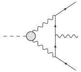
The leading-order diagram of the decay is shown in Fig. 1.
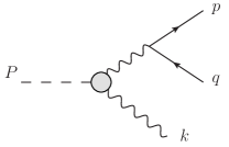
The shaded blob corresponds to the singly virtual electromagnetic transition form factor , which is closely related to the doubly virtual transition form factor by
| (4) |
The two-fold differential decay rate reads
| (5) |
Above, we have used the LO expression for the most prominent (electromagnetic) decay rate of a neutral pseudoscalar meson :
| (6) |
Integrating (5) over , we find the one-fold differential decay width
| (7) |
Moving beyond the leading order, it is convenient to introduce the NLO correction to the LO differential decay width, which allows us to write schematically . In particular, in the case of the two-fold differential decay width we define
| (8) |
and in the one-fold differential case we have
| (9) |
Concluding the definitions closely related to the previous work Husek et al. (2015), such a correction can be divided into three parts emphasizing its origin
| (10) |
Here, stands for the virtual radiative corrections, for the one-photon-irreducible contribution, which is treated separately from in our approach due to the reasons of historical development, and for the bremsstrahlung. As a trivial consequence of previous equations, having knowledge of allows for obtaining using the following prescription:
| (11) |
In the following sections we discuss the individual contributions one by one. We mainly point out the differences in comparison to the pion case.
III Virtual radiative corrections
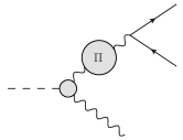
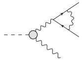
What we call the virtual radiative corrections is obtained from the interference terms of the LO diagram shown in Fig. 1 and the diagrams in Fig. 2a and 2b. In the pion case, the vacuum polarization was dominated by the electron loop. It turns out though that in the high-invariant-mass region of the photon propagator the hadronic effects become significant, which should be taken into account for the decays. Thus, in general, we shall deal with the photon self-energy in the form
| (12) |
where and stand for the leptonic and hadronic parts, respectively. We discuss these contributions separately in the following. At NLO, the contribution of the vacuum polarization (12) to the virtual radiative correction then reads
| (13) |
Note that does not depend on and consistently with (11) we have .
Regarding the lepton part, all the necessary formulae connected with the contributions of lepton loops to the vacuum polarization are stated in Section III of Husek et al. (2015) and hold also in the current cases. However, we shall point out some interesting details. It was already discussed in Husek et al. (2015) that in the case of the -meson decays not only the electron loop but also the muon loop should be taken into account as a part of the vacuum polarization contribution. The contribution of the leptonic vacuum polarization insertion — i.e. the contribution of the lepton loops to the photon propagator — to the correction can be expressed as (cf. the formulae in Section III of Husek et al. (2015))
| (14) |
Here, is the invariant mass of the final-state lepton pair and stands for the leptons circulating in the loop. Consistently with definition (2) we have and . Let us note that no longer stands for the CMS speed of the final-state leptons as was the case for in (2). Since depends on , which for the given process of a decay to a lepton pair of flavor satisfies the limit , we can run into different kinematical regimes, which are explicitly covered by formula (14); for this purpose the Heaviside step function was used. Whenever , i.e. itself becomes imaginary, no on-shell lepton-antilepton pair can be created in the loop and the diagram in Fig. 2a lacks the imaginary part. This happens if the invariant mass of the final-state lepton pair is under the production threshold of the two loop leptons of flavor : . In turn, this condition can be, of course, only realized in the case of the muon loop contribution to the NLO decay widths of the decay and in the process , where the kinematical condition is met within a part of the kinematically allowed region.
The hadronic contribution to the photon self-energy can be expressed via a dispersive integral Jegerlehner (1986)
| (15) |
Here, is the total cross section of the annihilation into hadrons and is related to the ratio as . In order to obtain a smooth curve from the data Patrignani et al. (2016), we fit the experimental values in a similar way as it was done in Jegerlehner (1986). Concerning the upper bound of the integral in (15), in practice it is sufficient to use the scale . It is set in such a way that all the important resonances are covered while the higher-energy region does not contribute significantly for . The resulting contribution to the radiative corrections is plotted as one of the constituent curves in Fig. 4.
Instead of (13), one might take into account the whole geometric series of vacuum polarization insertions and sum it in order to find
| (16) |
Eq. (13) is then recovered by taking the linear expansion of (16), since . Note that in (16) one should use a full form of the vacuum polarization including its imaginary part, similarly as it was e.g. defined in (20) of Husek et al. (2015) for the lepton case:
| (17) |
with But since , also and . One could thus safely use only the real part of , as it was defined in (13), for the purpose of the numerical evaluation of (16). This is equivalent to effectively using . On the other hand, the numerical difference between the definitions (13) and (16) is at . Therefore we take into account the precise formula (16) together with (15) and (17).
For completeness, let us revise at this point what we mean by the virtual correction. In agreement with Eq. (16) in Husek et al. (2015), we use
| (18) |
where contains not only single electron and muon loops, but also the whole hadronic contribution to the photon self-energy. For the form factors and , which arise from the vertex correction diagram in Fig. 2b, the reader is referred to seek the expressions in Husek et al. (2015).
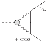
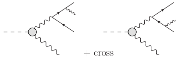
IV One-photon-irreducible virtual radiative correction
Considering the QED expansion, the NLO diagrams contributing to the one-loop one-photon-irreducible (1IR) correction to the process are shown in Figs. 2c and 2d. We treat this contribution separately from the virtual correction to emphasize the fact that it was not included in the original approach Mikaelian and Smith (1972a). Therein, it was considered to be negligible already for the pion case. This statement had been corrected in Ref. Tupper et al. (1983) many years before the debate about this issue was finally closed. Note also that in the pion case, the 1IR contribution was studied in Husek et al. (2014) in connection with the bremsstrahlung correction to the rare decay.
In the IR contribution one cannot factorize out the electromagnetic transition form factor. This correction becomes therefore unavoidably model-dependent already at the two-fold differential level and it is necessary to choose a particular model to evaluate the correction numerically. Compared to the previous calculations of the LO diagram and NLO virtual radiative corrections, a doubly virtual transition form factor is needed to be used. This form factor enters the loop and the integration over the unconstrained momentum is then performed. Note that stands for both the decaying pseudoscalar as well as for its four-momentum.
Let us now proceed further and consider that during the calculation of the 1IR loop diagrams the following structure inevitably appears:
| (19) |
By construction, the arguments of the form factor coincide with the photon propagators in the loop; denotes the loop momentum as is usual. In what follows we consider a family of large- motivated analytic resonance-saturation models, which are in detail discussed in Husek and Leupold (2015) ( denotes the number of colors). Here is a rational function with vector-meson poles. We then realize that due to a use of the partial fraction decomposition one can perform — within the loop integrals appearing during the evaluation of the diagrams — the following substitution:
| (20) |
Note that from now on we will suppress the explicit writing of the ‘+’ part. Above,
| (21) |
In this way we come from the matrix element to ; note that the normalization constant from decomposition (20) is already included in and that we have used a shorthand notation . In order to get results for the whole family of models it is necessary to analytically integrate over the loop momentum just once; this is the main advantage of this approach. At the end one can choose the particular model of the form factor by setting the parameters in the final matrix element appropriately. We can find the above used constants and from projecting on the product of the normalized form factor and the photon propagators: for instance in the case we have
| (22) |
This little trick is highly convenient when it is necessary to create a universal code for calculating radiative corrections within different models. Let us also note that substitution (21) does obviously not conserve term by term the desired property of the doubly virtual form factors — the symmetry in their arguments. This ansatz though works generally for the rational models mentioned above, which might have a rather complicated structure. The symmetry in question is then always restored in the final result after including all the pieces . Moreover, we realize that if we define
| (23) |
we can immediately write
| (24) |
This trivial observation simplifies the loop integration even further. Instead of (20), we can then write
| (25) |
During the calculation of the amplitude it is only necessary to perform the following substitution:
| (26) |
The desired final amplitude for the particular model is then obtained by writing a suitable combination (in spirit of (25)) of such amplitudes which are calculated using substitution (26). One only needs to insert the correct masses and coefficients into this combination, which goes along the lines of (24), (22) and (21).
Lets discuss the previous procedure on a particular case and consider for a while the eta-meson decays: . The simplest physically relevant model we can imagine is based on the VMD scenario, i.e. by an ansatz which assumes that the form factor is saturated by the lowest-lying multiplet of vector mesons. It has the following form:
| (27) |
Above, is the - mixing angle and together with are the associated decay constants in the quark-flavor basis of the quark currents Feldmann et al. (1999); Escribano and Frere (2005); for further details concerning derivation of this model see Appendix E. It is then clear after counting of the loop-momenta powers that such a form factor guarantees the UV convergence of the loop integrals. The matrix element for such a form factor can be schematically written as
| (28) |
Following the subsequent decomposition (24) and using linearity, one then finds
| (29) |
As the only building block, one needs to calculate obtained in terms of substitution (26) in the original matrix element. For the purpose of the 1IR contribution to the correction at the one loop level, the same decomposition will work. Indeed, an interference of with the LO matrix element needs to be considered and thus linearity is preserved. Therefore it is necessary to take into account a linear combination of defined according to the prescription (26) in Husek et al. (2015):
| (30) |
The explicit expressions for the building-block form factors and are shown in Appendix A. Let us have a look at the ratio of the electromagnetic form factors in (30). Clearly, irrespective of the model that we use for the doubly virtual form factor, it is convenient that the normalization of the form factor in such a model equals to appearing in the LO expression; see also (4). This leads to the fact that the correction will be independent of any overall normalization effects. In the next section we introduce a spectral representation of a normalized form factor; see (41). Following what we have just assumed, we can write
| (31) |
and using the VMD-based scenario for instance for as in (27), we find
| (32) |
A simple example of the presented approach applied on the decays is included as Appendix F. There is also a complementary technique how to cover a whole set of form factors under consideration. Instead of putting the particular form factor into our diagrams, we can use the local Wess–Zumino–Witten (WZW) term. In other words we trade the form factor for the constant given by the chiral anomaly. It is then clear from simple considerations, that the contributions from Fig. 2c need counter terms to compensate UV divergences. The convergent part of such a counter term carries an undetermined constant renormalized at scale , which can effectively mimic the high-energy behavior of the would-be complete form factor. Using a proper matching procedure, it is possible to acquire a numerical value of this constant for a given form-factor model. Up to mass corrections we can use an approximate formula to estimate this effective parameter (see Eq. (46) in Husek and Leupold (2015)). The question is, if this procedure can be used also for a box diagram in Fig. 2d which is already convergent for the local WZW form factor. It turns out that the corrections are of order and . Hence, for the pion case this assumption works well. On the other hand, for it does not and one would need to introduce additional effective parameters in a consistent way. This is though not a trivial task and is beyond the scope of this work. Let us also mention that enters the corrections being multiplied by and its effect is thus negligible for the decays with electrons in the final state.
In the result section (Section VI) we will use the simple VMD-inspired model for the doubly virtual transition form factor to estimate the importance of the 1IR contributions; for model details see Appendix E. For completeness, let us then present the correction within the model under consideration:
| (33) |
For the case, we have , . The case then corresponds to the simultaneous interchange {, }, of course followed by specifying the right within the building blocks . For the resonance masses we put (the average physical mass of and mesons) for the light sector and (the physical mass of the meson) for the strange sector. However, we would like to stress again that the framework presented in the present section is capable of dealing also with more sophisticated form-factor models. In general, the model dependence of part of the radiative corrections is, of course, a nuisance. But for the doubly virtual transition form factors of and there is at present no alternative. In the next section the singly virtual transition form factors are required. Here the model dependence can be reduced by the use of dispersive methods Hanhart et al. (2013, 2017).
V Bremsstrahlung
In this section we briefly build on Husek et al. (2015) — which among others discussed the bremsstrahlung correction calculation for the pion case — and show the differences which come into play due to the fact that we are now interested in mesons. We also show some techniques how to deal with the obstacles which arise. Concerning the notation, we will restrict ourselves to the one used in previous works.
The diagrams which contribute to the Dalitz decay bremsstrahlung are shown in Fig. 2e. Their contribution is (among others) important to cancel IR divergences stemming from the virtual corrections depicted in Fig. 2b. The corresponding invariant matrix element (including cross terms) can be written in the form
| (34) |
where
| (35) |
with
| (36) |
Here, we use and for the photons and and for the electron and positron four-momenta, respectively, and . Note that we use the shorthand notation for the product of the Levi-Civita tensor and four-momenta in which . Inasmuch as an additional photon comes into play it is convenient to introduce a new kinematical variable which stands for the normalized invariant mass squared of the two photons
| (37) |
It has the similar meaning as in the case of the lepton-antilepton pair. The contribution of the bremsstrahlung to the next-to-leading-order two-fold differential decay width can be written as
| (38) |
The above used operator is defined for an arbitrary invariant of the momenta and as follows:
| (39) |
In the case of the pion Dalitz decay, the value of the slope parameter of the form factor is small: . Consequently, the form factor which enters (34) can be conveniently expanded in the following way:
| (40) |
Therefore, can be approximated by for the process . This squared leads to the direct cancellation with appearing in the leading-order expression. The bremsstrahlung contribution to the radiative corrections then becomes effectively independent of the particular model of the pion transition form factor. However, in the case of an meson, the slope parameter is , which is definitely not negligible anymore. One would need to include higher-order corrections in expansion (40), the convergence would be slower and things would become in general more complicated since additional terms would need to be treated; see also the discussion at the end of Section V of Husek et al. (2015). The real obstacles though appear with the -meson case. Due to the fact that , expansion (40) is not applicable at all. One thus needs to calculate with the full form factor.
Although in such a case the situation is somewhat different compared to the one in which the form factor cancels out, in general it is possible to use a similar framework as in the pion case — at least in the sense of treating the kinematical integrals. Accordingly, one needs to rewrite the bremsstrahlung correction in terms of integrals which are known from the pion case. These need to be somewhat generalized due to the presence of poles in the form factor; for results see Appendix C. This becomes more important in the case compared to the pion decay and needs to be taken into account explicitly. For the case, this procedure then becomes absolutely crucial since in the hadron spectrum the mass of the meson lies above the masses of the lightest vector-meson resonances and and close to the -meson mass. The subsequent (numerical) integrations over all the relevant kinematical configurations of the bremsstrahlung photon become significantly nontrivial due to the running over these poles, which are regulated by incorporating physical widths of the resonances. The narrow resonances like and are somewhat straightforward to include. However, the width of the broad resonance is sensitive to the - scattering. This can be also taken into account by the use of recent dispersive approaches Hanhart et al. (2013, 2017). To this extent, it is convenient to use the Källén–Lehmann spectral representation of the Feynman propagator, which allows for the use of a common spectral density function for all the mentioned resonances. The facts stated above make the bremsstrahlung contribution — especially in the case of the meson — significantly sensitive to the form-factor model. To minimize the model dependence, whenever possible, data and general principles of QFT, analyticity and unitarity, are used that give rise to a dispersive framework.
In the Källén–Lehmann spectral representation, the form factor has the following form:
| (41) |
Concerning the integration range, we restrict ourselves to . This is sufficient for our purpose and covers all the important physics. In the lower bound, is the mass of a charged pion and then constitutes the squared mass of the lowest hadronic state that can couple to a photon. The upper bound is governed by the cut-off GeV chosen in such a way just to cover the peak and width of the resonance. The spectral function has in the chosen energy range two main contributions distinguished by isospin, .
The narrow resonances and contribute to the isospin-zero part
| (42) |
with the narrow-resonance spectral function
| (43) |
Note that after a full integration over one indeed gets (up to a sign) the resonance propagator:
| (44) |
Finally, let us mention, that a one-narrow-resonance VMD model for the form factor can be written in terms of (41) with .
The isospin-one part is governed by the broad meson. In order to include the important effect of scattering, we use the dispersive approach of Hanhart et al. (2013, 2017). There the spectral function has the form
| (45) |
where MeV is the pion decay constant, is the Omnès function, a dispersive tool incorporating pion rescattering, and and are polynomials related to the reaction amplitude and the pion vector form factor , respectively. In the case of , we use with and Hanhart et al. (2017). For the spectral function, we take (based on Hanhart et al. (2013)) with . Note that in view of (45) and taking into account only terms linear in , . The rest of the parameters from (42) and (45) are given in Table 1.
| [GeV-2] | ||||
|---|---|---|---|---|
| 0.56 | 0.115 | 0.78(4) | 0.75(3) | |
| 0.415 | 0.09 | 1.27(7) | 0.54(2) |
For numerical reasons, the spectral function for the broad resonance may be fitted, since it is much faster to numerically integrate the analytical expression compared to the dispersive data interpolation. To this extent, it is necessary to model the resonance peak behavior. The following function copies the dispersive shape of satisfactorily:
| (46) |
The energy dependence of the width of the meson — assuming the main contribution comes from the 2-decay — can be expressed as
| (47) |
The advantage of the latter approximation is the fact, that when we insert it into (46) and subsequently into (41), the form factor can be evaluated analytically. This speeds up the numerics even further. The values of the fit are shown in Table 2.
| [GeV-2] | [GeV-2] | [GeV-2] | ||
|---|---|---|---|---|
| 3.336 | -6.364 | 2.622 | -1.342 | |
| 2.333 | -4.969 | 2.261 | -1.240 |
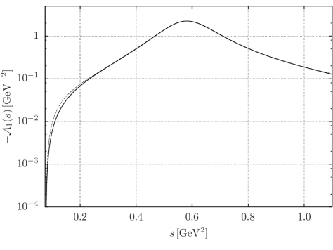
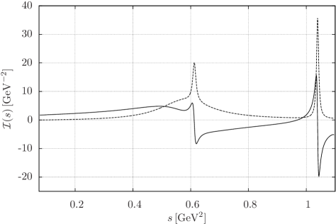
For the case, the formula (45) is compared to the fit in the upper panel of Fig. 3. The dispersive integral of the final spectral function is then shown in the second panel of Fig. 3.
Let us now show, how the matrix element squared looks like in the spectral representation. For the sake of writing down its structure, we recast (34) as
| (48) |
where we have used the shorthand notation and and defined and . After inserting the representation of the form factor (41) we get
| (49) |
An attentive reader might have noticed that in the previous formula the explicit is not necessary. At the same time, it might be sensible to explicitly write the infinitesimal imaginary part of the propagator in the following expressions. To avoid any potential confusion further on, let us define and, similarly, . After the operator is applied on the matrix element squared and summed over all the spins and polarizations , we can actually use the symmetry term by term, which results into
| (50) |
In order to perform the integrations of the operator on the respective terms, we need to do a few fraction-product decompositions; the procedure is described in detail in Appendix D. Taking also into account that
| (51) |
we can rewrite (50) into
| (52) |
Following the definition (41), we made use of the fact that
| (53) |
With the previous simplifications (43), (46) and (47), the above integral can be evaluated analytically which speeds up the time-demanding numerics.
For the sake of integrating out the bremsstrahlung photon it is convenient to define the following three rescaled parts of the matrix element squared:
| (54) | ||||
| (55) | ||||
| (56) |
One gets the remaining building blocks of (52) by performing the limit , i.e. taking and . Note that it does not matter if one uses or simply for the Feynman propagators in the definitions of and since these give real contributions. The name Tr is chosen to be in agreement with Mikaelian and Smith (1972a). Note that the original work of Mikaelian and Smith (M&S) — which in some sense corresponds to since the form factor could have been factorized out — is connected with the previous definitions through
| (57) |
where
| (58) |
For numerical reasons, the integration of the resulting expression is performed term by term. We can name these terms for further convenience. Consequently, we write
| (59) |
where
| (60) | ||||
| (61) | ||||
| (62) | ||||
| (63) |
Terms and are the only ones present in the M&S case. Terms and are dominant. By construction (cf. (116)), terms and belong together since separately they develop peaks which are exactly compensated only in the sum. Let us mention that for the purpose of (59), in it is sufficient to take only the real part of since gives only a real-part contribution.
For the correction it holds
| (64) |
Together with (116) this suggests that we need to perform five subsequent integrations: two nontrivial analytical ones are implicitly hidden in the operator and at least two need to be inevitably performed numerically. Let us briefly look at the explicit integral structure — for instance on the case of — and how it contributes to the bremsstrahlung correction. In terms of definitions (53) and (56) we have
| (65) |
The term can be evaluated analytically by taking the fit (46) of the spectral function instead of its numerical form (45) given by the term containing the Omnès function. This procedure significantly speeds up the numerics. The evaluation of is performed analytically and the strategy is similar to the one used in Husek et al. (2015). Our goal is to rewrite the expressions under consideration into basic integrals, which are then listed in Appendix D of Husek et al. (2015) and Appendix C of the presented work. For this purpose, symmetries and properties of operator are used together with the reduction procedure described in detail in Section V of Husek et al. (2015) and summarized in Appendix B therein. Due to the presence of the effective mass in the denominators, this procedure needs to be slightly modified since now also appears instead of simple . As a trivial example, we choose the following reduction:
| (66) |
Note also that the IR-divergent terms (those which diverge after integrating over ) need to be treated separately. The current case is discussed in Appendix B. For further details and an introduction we refer an interested reader to Husek et al. (2015).
To conclude, let us finally write the bremsstrahlung contribution to the radiative corrections (cf. (37) in Husek et al. (2015)):
| (67) |
where index runs over all the subscripts appearing in definitions (60)-(63): 1a, 1b (the form-factor-independent parts) and 2, 3a, 3b and 4 (the form-factor-dependent parts).
VI Results
In the previous sections, we discussed the three main parts of radiative corrections as we referred to them in (10), i.e. the virtual corrections in Section III, the 1IR correction in Section IV and the bremsstrahlung in Section V. In order to get the final result, one then simply sums over the partial results: Eqs. (18), (33) and (67). Let us now comment once again on these contributions in detail. The model-independent expression for the virtual corrections (18) includes the photon self-energy contribution (12), consisting of the exact (at NLO) leptonic (17) and the experimental-data-based hadronic (15) parts, and the vertex correction expressed in terms of the and form factors. The expressions for these form factors can be found in Husek et al. (2015); in particular see Eqs. (22) and (23) therein. The form factor then contains the IR-divergent piece which cancels with the corresponding term stemming from the bremsstrahlung contribution, as shown at the end of Appendix B. The bremsstrahlung contribution (67) itself consists of the fully model-independent ingredients (60), already present in the M&S case, and the pieces (61-63) that still contain some model dependence, though mitigated by our dispersive, data-driven input. All the necessary definitions are then presented in Appendices B and C. Finally, for the model-dependent 1IR contribution (33) we used the VMD-inspired model discussed in Appendix E. Let us again stress at this point that we used a rather general approach applicable for a wide family of rational models. The final result within a particular model can then be found as an appropriate linear combination of the building blocks (30), with the form factors and defined in Appendix A. As another example of a suitable model we mention the one based on the Resonance Chiral Theory framework Guevara et al. (2018). There are other — data-driven — models Escribano and Gonzàlez-Solís (2018); Masjuan and Sanchez-Puertas (2017), which are then not directly applicable using the presented approach. However, we expect that different models would lead to compatible values in the numerical results.
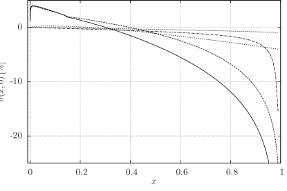
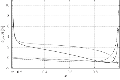
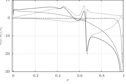
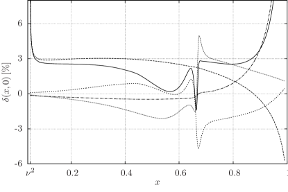
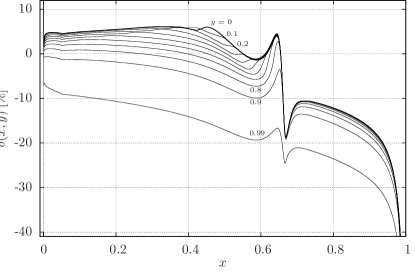
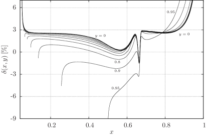
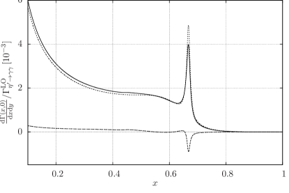
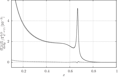
The overall NLO radiative corrections to the two-fold differential decay widths and their comparison to the main constituents are shown, for the case , in Fig. 4. In light of a direct comparison of our results for the process to the previous work Mikaelian and Smith (1972b), we can mention a significant difference between both approaches. Taking into account all the discussed contributions, a table of values of corrections to the process similar to the one provided in the original work Mikaelian and Smith (1972b) can be produced at the very same points; see Table 3. The difference can then be seen even more explicitly when comparing directly the corresponding values in Table 3 with Table I in Mikaelian and Smith (1972b). In the same manner, values for the decay are presented in Table 4. From the plots in the bottom panels in Fig. 4 we can see that for the case of an meson, such a table would need to be much denser to cover the wiggle behavior. For this reason, the table-like plots were created, which show the overall NLO radiative corrections for various values of ; see Fig. 5. To fully complement these figures, the standard tables of values, where the wiggle region is left out, are provided likewise; see Tables 5 and 6.
In Fig. 4 we can see that the 1IR correction has an intriguing character. For the decays it is negative for the whole range of values of and enhances thus the effect of the M&S-like corrections which are also negative in a wide range of . On the other hand, for the process the situation is different due to higher masses involved. In this case, is very close to zero, mostly slightly negative, but then it starts to be significantly positive. Its dominant behavior for large contributes to the fact that is positive over nearly the whole range of .
The form-factor effects are significant and shown in Fig. 4 as large-spaced dotted lines. Out of these contributions, is most prominent and responsible — together with the hadronic part of the vacuum polarization — for the wiggles in the case of decays. The terms and are on the other hand — although being most complicated and time consuming to calculate — rather suppressed. Together with another numerically small contribution to the bremsstrahlung correction, , they can be even considered negligible in the case of the . In the case of the decays into electrons, the considered correction is of order 0.1 % for small , otherwise negligible, too. Except for the already mentioned form-factor-dependent term , there is then only one significant contribution to the bremsstrahlung correction , which comes with its separately treated IR-divergent counterpart .
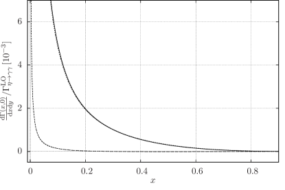
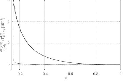
In order to fully understand the effect of the amusingly looking wiggles showed in Fig. 4 and Fig. 5 and eventually appreciate the size of the calculated radiative corrections, we present the differential decay widths in Fig. 6. In these plots, we can see a direct comparison of the LO and NLO decay widths, together with their sum. In general, the total radiative corrections look rather negligible, with an exception of the process . In this case, the corrections are significant and the NLO differential decay width is sizable compared to the LO width. The wiggles, which appear only in the case, then contribute in such a way that they change the shape of the resonance peaks and make them smaller. In particular, Fig. 6c shows that the height of the peak is considerably influenced by the radiative corrections. This might be interesting for the extraction of properties or of the - interplay. One might deduce such information from or from . It can be expected that the radiative corrections are different for these two decay branches. Ignoring such radiative corrections in the analyses of these decays might lead to contradictory conclusions.
Finally, let us shortly mention that the hadronic part of the vacuum polarization has, in contrary to the case, a significant impact on the corrections for the decays, with up to a 5 % effect in the region.
Acknowledgment
T.H. would like to thank Uppsala University and University of Birmingham for their hospitality. We would also like to thank A. Kupść for providing us with the Omnès function data used in Hanhart et al. (2017).
This work was supported by the Czech Science Foundation grant GAČR 18-17224S and by the ERC starting grant 336581 “KaonLepton”.
| 0.01 | |||||||||||
|---|---|---|---|---|---|---|---|---|---|---|---|
| 0.02 | |||||||||||
| 0.03 | |||||||||||
| 0.04 | |||||||||||
| 0.05 | |||||||||||
| 0.06 | |||||||||||
| 0.07 | |||||||||||
| 0.08 | |||||||||||
| 0.09 | |||||||||||
| 0.10 | |||||||||||
| 0.15 | |||||||||||
| 0.20 | |||||||||||
| 0.25 | |||||||||||
| 0.30 | |||||||||||
| 0.35 | |||||||||||
| 0.40 | |||||||||||
| 0.45 | |||||||||||
| 0.50 | |||||||||||
| 0.55 | |||||||||||
| 0.60 | |||||||||||
| 0.65 | |||||||||||
| 0.70 | |||||||||||
| 0.75 | |||||||||||
| 0.80 | |||||||||||
| 0.85 | |||||||||||
| 0.90 | |||||||||||
| 0.95 | |||||||||||
| 0.99 |
| 0.15 | ||||||||||
|---|---|---|---|---|---|---|---|---|---|---|
| 0.16 | ||||||||||
| 0.17 | ||||||||||
| 0.18 | ||||||||||
| 0.19 | ||||||||||
| 0.20 | ||||||||||
| 0.21 | ||||||||||
| 0.22 | ||||||||||
| 0.23 | ||||||||||
| 0.24 | ||||||||||
| 0.25 | ||||||||||
| 0.30 | ||||||||||
| 0.35 | ||||||||||
| 0.40 | ||||||||||
| 0.45 | ||||||||||
| 0.50 | ||||||||||
| 0.55 | ||||||||||
| 0.60 | ||||||||||
| 0.65 | ||||||||||
| 0.70 | ||||||||||
| 0.75 | ||||||||||
| 0.80 | ||||||||||
| 0.85 | ||||||||||
| 0.90 | ||||||||||
| 0.95 | ||||||||||
| 0.99 |
| 0.01 | |||||||||||
|---|---|---|---|---|---|---|---|---|---|---|---|
| 0.05 | |||||||||||
| 0.10 | |||||||||||
| 0.15 | |||||||||||
| 0.20 | |||||||||||
| 0.25 | |||||||||||
| 0.30 | |||||||||||
| 0.35 | |||||||||||
| 0.40 | |||||||||||
| 0.45 | |||||||||||
| 0.50 | |||||||||||
| 0.55 | |||||||||||
| 0.60 | |||||||||||
| 0.70 | |||||||||||
| 0.75 | |||||||||||
| 0.80 | |||||||||||
| 0.85 | |||||||||||
| 0.90 | |||||||||||
| 0.95 | |||||||||||
| 0.99 |
| 0.05 | |||||||||||
|---|---|---|---|---|---|---|---|---|---|---|---|
| 0.10 | |||||||||||
| 0.15 | |||||||||||
| 0.20 | |||||||||||
| 0.25 | |||||||||||
| 0.30 | |||||||||||
| 0.35 | |||||||||||
| 0.40 | |||||||||||
| 0.45 | |||||||||||
| 0.50 | |||||||||||
| 0.55 | |||||||||||
| 0.60 | |||||||||||
| 0.70 | |||||||||||
| 0.75 | |||||||||||
| 0.80 | |||||||||||
| 0.85 | |||||||||||
| 0.90 | |||||||||||
| 0.95 | |||||||||||
| 0.99 |
Appendix A Matrix element of the one-photon-irreducible contribution
The building-block matrix element for the one-photon-irreducible contribution can be expressed in terms of scalar form factors in the following (manifestly gauge-invariant) way (cf. (24) in Husek et al. (2015)):
| (68) |
The form factor does not contribute to , so we do not include it in this appendix. Note also that only the box diagram (see Fig. 2d) contributes to . Let us also define the two-point (bubble) scalar one-loop integral as a reference point for the used notation:
| (69) |
Above, we have introduced . Before providing the final expressions, let us define
| (70) | ||||
| (71) |
Using the dimensional regularization, the dimensional reduction scheme Siegel (1979); Novotný, J. (1994)) and Passarino–Veltman reduction Passarino and Veltman (1979), the explicit results for the two contributing form factors, and , in terms of scalar one-loop integrals read (we use again for simplicity , and )
| (72) |
| (73) |
Appendix B Bremsstrahlung matrix element squared
In this appendix we provide explicit formulae for the building blocks of the bremsstrahlung invariant matrix element squared, as described in Eqs. (52-63). If we generalize (54) to
| (74) |
we only need to provide its explicit form in order to cover and defined in (54) and (55). Indeed, one can obtain by means of multiplying by the appropriate propagator: . For completeness, .
In the following expressions, as denoted below, the symmetries of the operator were already taken into account and the reduction procedure (in the sense of Appendix B of Husek et al. (2015)) into the basic integrals was performed as well. Before we get to the desired expressions, we need to define a complete set of the Feynman denominators (while suppressing the ‘+’ part):
| (75) |
For simplicity, in what follows we use , and . The term which includes squares of the bremsstrahlung diagrams reads
| (76) |
the IR-divergent part of which, up to and the part, is given as
| (77) |
This is in agreement with Appendix A of Husek et al. (2015) up to an additional factor of 1/2 visible in matching (58). Above, we have used the following definitions:
| (78) | ||||
| (79) | ||||
| (80) | ||||
| (81) | ||||
| (82) |
The second building block which arises from the interference of bremsstrahlung diagrams under consideration can be expressed as
| (83) |
where we have defined the function
| (84) |
Needless to say, whenever appears above it applies for entire expressions. Let us note that after inserting the expressions (76) and (83) into formula (58), one indeed recovers expressions presented in Appendix A of Husek et al. (2015).
In (59), which we can reformulate into
| (85) |
only and contribute to the overall IR-divergent part, which can be rewritten as
| (86) |
We already know that ; note that . In addition, by definition, the IR-divergent part of is given by the divergent part of . To this, only can contribute. Moreover, we realize that and that only its part does not suppress the essentially divergent terms and appearing in . Consequently, . We thus find
| (87) |
which, using (78) and (41), translates into
| (88) |
Due to the symmetries of the double integral and the fact that in the end we are nevertheless interested only in the real part, the term in the square brackets can be further recast into
| (89) |
Taking the real part of the previous result, we finally get (cf. definition (41))
| (90) |
The form factor squared cancels after normalizing on the LO differential decay width and, subsequently, we get the same as in Husek et al. (2015), Appendix A. This is the desired result, since contains the terms which exactly cancel the IR divergences stemming from the virtual corrections: is then IR-safe.
Let us recall that the integration of over needs to be performed analytically. Note that it was only kept as a part of since it also contributes to the IR-convergent part of .
Appendix C Basic terms
In this appendix we provide a list of integrals generated by acting of operator , which are not covered by Appandix D in Husek et al. (2015). These appear as a consequence of the generalization of the bremsstrahlung matrix element, which was necessary in our current approach. This is connected to the fact that we took the effect of vector-meson resonances into account. First, let us recall that
| (91) | |||
| (92) |
and define
| (93) |
Next, we define functions , and in the following manner:
| (94) |
| (95) |
where with
| (96) | ||||
| (97) | ||||
| (98) |
and finally
| (99) |
Furthermore, with the definitions
| (100) | ||||
| (101) |
at hand, we can express the missing basic integrals as
| (102) | ||||
| (103) | ||||
| (104) | ||||
| (105) | ||||
| (106) |
where we have used and . Note that (106) includes an IR-divergent part . Let us also mention that even though it might seem like that after inspecting definition (76) of , it is not necessary to define other integrals, e.g.
| (107) |
since only and appear in the final expression for . For completeness, let us take advantage of our notation and add that . All the other terms can be found in Appendix D of Husek et al. (2015). At this point, let us mention that in Husek et al. (2015), terms (D20) and (D21) were not listed properly in light of definition (D1). It was not stated explicitly that the second version of (D1) was used for evaluating all the terms. This (second) version, however, equals to the original definition
| (108) |
only for , as mentioned in (D1). When , an additional overall minus sign appears. This was not emphasized and shall at least be clarified at this point. Taking thus into account (108), which is universal for any , we find
| (109) | ||||
| (110) |
Other expressions in Appendix D of Husek et al. (2015) require no changes. Let us also mention that one should indeed get now (109) by putting in (104).
Appendix D Partial fraction decompositions for the bremsstrahlung matrix element squared
In this appendix we show how to rewrite the bremsstrahlung matrix element squared (50) into a form which will allow us to perform the integrations of the operator on the respective terms. To achieve this we need to use a few fraction-product decompositions. First, we take the simplest case:
| (111) |
Note that represents a Feynman denominator corresponding to the virtual photon and in this and following applications the difference between and plays no role. We also write instead of since due to the positive limits of the integration. Similarly,
| (112) |
In the denominators, and represent positive and infinitesimally small independent numbers and the numerical result remains the same even when we assume for simplicity that . Now, we can use the fact that this term is multiplied by two spectral functions and and integrated symmetrically over and . After we rename in the second term on the right-hand side of (112), we realize that due to the symmetric integration we obtain the complex conjugate of the first term. Since we are anyway interested in the real part only, we just get the factor of 2. In the following we use the knowledge of the fact that is a significant -invariant combination of kinematical variables:
| (113) |
Note that due to the presence of the operator, we can substitute by on the right-hand side of the previous equation. Above, is actually artificial and can be safely sent to zero. This can be also seen due to some other reasons. First, on the left-hand side we could have already written instead of . Another, more general, reasoning is similar to the following case. The last term which needs to be treated can be decomposed as
| (114) |
Again, and are infinitesimally small and independent. For a moment we can assume these to be finite though small. The left-hand side does obviously not depend numerically on the fact if is greater or smaller than so the apparent dependence of this type needs to be canceled on the right-hand side. For this purpose both of the terms in the brackets are necessary. Without loss of generality we can assume that and put with small. Since and can be arbitrary for (114) to be valid, we can set . In the corresponding limit we can apply the Sochocki’s formula to find
| (115) |
where stands for the principal value. The part containing the delta function then trivially vanishes (due to the first bracket) together with the dependence on the sign of the difference . Again, using the fact that the integration is symmetric in and and that we can on the right change , we obtain the sum of a term and its complex conjugate, which results in a factor of 2 under the real-part operator; note that has no (nonvanishing) imaginary part since it is related to the tree diagram.
Appendix E VMD-inspired model for the electromagnetic transition form factors
E.1 Introduction
For a phenomenological model of a transition between the meson and virtual photons we need to take into account a strange-quark content of . It is more convenient to work in the quark-flavor basis than in the octet-singlet one Feldmann et al. (1999); Escribano and Frere (2005). In such a basis, the vector currents related to physical states of , and mesons are identical to the basis currents. Having a standard definition of vector currents and pseudoscalar densities in the octet-singlet basis111Our convention is .(note that )
| (117) |
we can write for the currents of our interest
| (118) | ||||||
| (119) | ||||||
| (120) |
Note that for simplicity we have left out the spacetime coordinates of the currents and quark fields. Above, we see the relations between neutral-meson-related vector currents, appropriate combinations of quark-flavor-diagonal vector currents, their octet-singlet basis decomposition and finally the quark-flavor basis definition. The electromagnetic current reads
| (121) |
In the chiral limit, the correlator is defined in the octet-singlet basis by
| (122) |
with . In the above formulae we have used
| (123) |
As it is common, where denote the Gell-Mann matrices in the flavor space and are the symmetric symbols.
If, for simplicity, we rewrite (122) schematically as
| (124) |
then — using linearity and definitions (118), (119) and (120) — we get only three nontrivial combinations of currents in the quark-flavor basis:
| (125) | ||||
| (126) | ||||
| (127) |
In this way we have found the normalization relation among bases (there is an additional factor in the case of the strange correlator). Note that and . In Eqs. (125)-(127) we have gone beyond the chiral limit: from now on we will distinguish between the light and strange correlators.
Since the quark content of the physical states is not equal to the isoscalar states, there is a mixing between and mesons. In the quark-flavor basis, this mixing occurs (for ) among the states defined as together with the orthonormality relation . The resulting mixing (in the quark-flavor basis) can be written as
| (128) | ||||
| (129) |
Next we define the correlator for each basis state (again ):
| (130) |
The factors are related to the pion case by : we have introduced the ratio of the decay constants . For the correlator we can then finally write
| (131) |
The factor comes from (127) and the mixing factors from (128). To avoid difficulties connected with calculation of the decay constant values and defining the final correlator all the way through (130), we will use the VMD ansatz
| (132) |
where the light and strange channels are saturated by associated resonances: and .
Numerical values for the mixing angle and decay constants and are obtained from various experimental data (for details see next part of this appendix) in terms of a global fit with the result
| (133) |
These values are used throughout the paper.
E.2 Model relevancy check
Now we have to check if such a VMD-inspired model is phenomenologically successful and if it is suitable for calculating 1IR contribution to the NLO virtual radiative corrections.
E.2.1 Decays including vector mesons
We may start with processes containing vector mesons. To investigate this we need to take into account few more quantities. We now introduce the overlap between a meson () and the vector current , i.e.
| (134) |
Here we assume that and mesons contain only the light quarks (no hidden strangeness) and the meson contains only the strange quarks. This is a fairly good approximation to the real world Patrignani et al. (2016). For later convenience we also define the - coupling strength . With this at hand we can obtain from the decay processes. The direct calculation from the Lorentz invariant matrix element
| (135) |
yields in the limit after averaging and summing over polarizations
| (136) |
Above, is the overlap of the electromagnetic current with the meson-related current , For a little more details concerning the case see Husek and Leupold (2015). Necessary numerical inputs and results are shown in Table 7.
| [MeV] | 782.65(12) | 775.26(25) | 1019.46(2) |
|---|---|---|---|
| [MeV] | 8.49(8) | 147.8(9) | |
| [] | 7.28(14) | 4.72(5) | 29.54(30) |
| /3 | /3 | ||
| [keV] | 0.62(2) | 7.0(1) | 1.26(2) |
| [MeV] | 140(2) | 156(2) | 161(1) |
For the following, it is convenient to introduce the correlator
| (137) |
Consequently, the form factor within the VMD model can be written as
| (138) |
The additional factors , which come from the - mixing, can be found in Tabs. 8-9. Using these form factors we can calculate the two-body decay widths containing one pseudoscalar meson (), one vector meson (, or ) and one photon. Depending on the masses of the particles involved, we use one of the following two prescriptions:
| (139) |
| (140) |
The results together with a comparison with the experimental data can be found, for the case, in Table 8, and for the case in Table 9.
| 6.6(1.7) | 3.0(2) | 130.9(2.4) | |
| [keV] | 5.6(1.4) | 44(3) | 56(1) |
| [keV] | 5.7(7) | 37(5) | 50(5) |
| 2.75(23) | 29.1(5) | ||
| [keV] | 5.4(5) | 58(3) | 0.27(1) |
| [keV] | 6.5(9) | 52(7) | 0.30(2) |
We see that the VMD model and the experimental data are in agreement.
The last class of the processes containing vector mesons which we will investigate is a counterpart of the previous decays, when the photon in the final state is virtual and turns into the lepton pair. The decay width can then be expressed as a form-factor-dependent integral over the dilepton invariant mass
| (141) |
where denotes the Källén triangle function defined as
| (142) |
After inserting numerical values we get
| (143) |
which should be compared with . For the above evaluation we have used Patrignani et al. (2016).
Data for and decays as well as for and decays are not available.
E.2.2 Electromagnetic transition form factor
Using previously defined meson-specific factors, we can finally define the doubly virtual electromagnetic transition form factor of an eta meson in the quark-flavor basis:
| (144) |
For above we simply substitute and . In the VMD case (inserting ansatz (132)) the form factor becomes
| (145) |
To get the form factor, it is only necessary to perform the following substitution:
| (146) |
As a simple application, we can have a look at the two-photon decay of a pseudoscalar . The decay with of such a process can be expressed as follows:
| (147) |
Of course, for a neutral pion we would have . In the case we can write
| (148) |
which becomes (cf. (145) for )
| (149) | ||||
| (150) |
Note that e.g. is consistent with experiment, although it differs significantly from a naïve WZW-based calculation Savage et al. (1992) for which . The results are shown in Table 10.
| [MeV] | 547.862(17) | 957.78(6) | |
|---|---|---|---|
| [keV] | 1.31(5) | 198(9) | |
| [%] | 39.41(20) | 2.20(8) | |
| [keV] | 0.52(2) | 4.4(2) | |
| [keV] | 0.52(8) | 4.2(5) |
We see that there is a very good agreement between the prediction of the VMD model and the experimental results.
Next, we should investigate the singly virtual transition form factor. One possibility is to compare the decay widths of the Dalitz decays. These can be written as the following integral:
| (151) |
A simple model we discuss here is however (in the singly virtual mode) not suitable for the Dalitz decays of due to the unregulated pole which needs to be integrated over. We thus present results only for the case. These are shown in Table 11.
| process | |||
|---|---|---|---|
| 69(4) | 3.1(4) | ||
| [eV] | 9.0(6) | 0.41(6) | |
| [keV] | 8.6(2.0) | 0.41(8) |
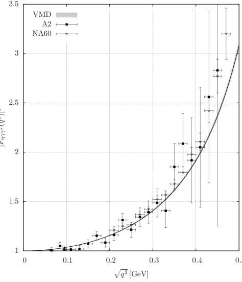
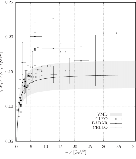
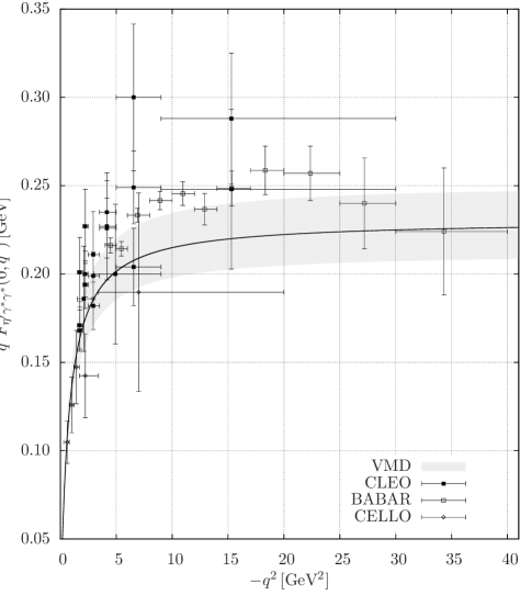
The other way is to directly plot the transition form factor over the respective data. The measurements of the transition form factor in time-like region are shown in Fig. 7. In the space-like region the results can be found in Fig. 8.
Finally, we can test the transition form factor in its whole power, in the doubly virtual mode. Using the VMD model (145), we can calculate the decay width of one of the rare processes . Note that data for the rare processes and are not available yet; for predictions for these decays within the model under discussion see Table 12 in Appendix F. Experimentally, the branching ratio was found to be , which translates into keV. Within the VMD model we find keV, which is in agreement with the experimental value. Note that we have calculated this value using the convenience of the approach shown in the following appendix. It is similar to the one we have used to calculate the 1IR contribution to the radiative corrections in Section IV. Finally, let us also mention that for the decays under consideration, more advanced models were developed Masjuan and Sanchez-Puertas (2016), which could also mimic rescattering effects.
Appendix F Form factors in decays
In this appendix we apply the approach explained in Section IV to the decays. We would like to show how the building block for the matrix element looks like in this case and calculate the coefficients for the specific transition form-factor models.
On account of the Lorentz symmetry and parity conservation, the on-shell matrix element of the process can be written in terms of just one pseudoscalar form factor in the following form:
| (152) |
Subsequently, the decay width reads
| (153) |
Taking into account only the LO contribution in the QED expansion, we find for the pseudoscalar form factor
| (154) |
Here, and , where and are the lepton momenta and is the triangle Källén function. For the rational resonance-saturation models, we will use in agreement with substitution (20) the following definition:
| (155) |
In the case of the process within the VMD model discussed in Appendix E, we can write (cf. (145))
| (156) |
Note that in the pion case we would simply have
| (157) |
After recalling (29) we know that the previous expressions might be obtained in terms of linear combinations of the building blocks . Using the dimensional regularization, the dimensional reduction scheme Siegel (1979); Novotný, J. (1994) and Passarino–Veltman reduction Passarino and Veltman (1979), the explicit result of the necessary loop integration in terms of scalar one-loop integrals reads
| (158) |
Above, it was convenient to introduce the following combination of the three-point scalar one-loop function and the Källén triangle function :
| (159) |
For completeness, we list the predictions for the branching ratios of the decays in Table 12.
In what follows, we would like to provide some basic examples of the decomposition of the loop integrals containing various models for transition form factors in the case of the rare decay of a neutral pion. Lets start with some definitions. The VMD ansatz for the electromagnetic transition form factor of a neutral pion takes a simple form
| (160) |
The lowest-meson dominance (LMD) model Knecht et al. (1999), where also the lowest-lying pseudoscalar multiplet was taken into account, gives the following result:
| (161) |
As the last example we introduce the two-hadron saturation (THS) model proposed in Husek and Leupold (2015), which for the correlator takes into account two meson multiplets in both vector and pseudoscalar channels:
| (162) |
In terms of decomposition (20) we can write for the amplitudes
| (163) | ||||
| (164) | ||||
| (165) | ||||
where the coefficients and have the following form:
| (166) | ||||
| (167) | ||||
| (168) | ||||
| (169) | ||||
We can find the above-listed constants from projecting on the product of the normalized form factor and the photon propagators: for instance we have
| (170) |
Taking into account decomposition (25) into building blocks (158), one recovers formulae (A.5-A.7) from Husek and Leupold (2015).
References
- Husek et al. (2015) T. Husek, K. Kampf, and J. Novotný, Phys. Rev. D92, 054027 (2015), arXiv:1504.06178 [hep-ph] .
- Lazzeroni et al. (2017) C. Lazzeroni et al. (NA62), Phys. Lett. B768, 38 (2017), arXiv:1612.08162 [hep-ex] .
- Mikaelian and Smith (1972a) K. Mikaelian and J. Smith, Phys. Rev. D5, 1763 (1972a).
-
Hanhart et al. (2013)
C. Hanhart, A. Kupść, U. G. Meißner, F. Stollenwerk, and A. Wirzba, Eur. Phys. J. C73, 2668 (2013),
Erratum: Eur. Phys. J. C75, 242 (2015), arXiv:1307.5654 [hep-ph] . - Hanhart et al. (2017) C. Hanhart, S. Holz, B. Kubis, A. Kupść, A. Wirzba, and C. W. Xiao, Eur. Phys. J. C77, 98 (2017), arXiv:1611.09359 [hep-ph] .
- Mikaelian and Smith (1972b) K. O. Mikaelian and J. Smith, Phys. Rev. D5, 2890 (1972b).
- Silagadze (2006) Z. K. Silagadze, Phys. Rev. D74, 054003 (2006), arXiv:hep-ph/0606284 [hep-ph] .
- Fang et al. (2018) S.-s. Fang, A. Kupść, and D.-h. Wei, Chin. Phys. C42, 042002 (2018), arXiv:1710.05173 [hep-ex] .
- Adlarson et al. (2017) P. Adlarson et al., Phys. Rev. C95, 035208 (2017), arXiv:1609.04503 [hep-ex] .
- AlekSejevs et al. (2013) A. AlekSejevs et al. (GlueX), (2013), arXiv:1305.1523 [nucl-ex] .
- Kubis and Schmidt (2010) B. Kubis and R. Schmidt, Eur. Phys. J. C70, 219 (2010), arXiv:1007.1887 [hep-ph] .
- Jegerlehner (1986) F. Jegerlehner, Z. Phys. C32, 195 (1986).
- Patrignani et al. (2016) C. Patrignani et al. (Particle Data Group), Chin. Phys. C40, 100001 (2016).
- Tupper et al. (1983) G. B. Tupper, T. R. Grose, and M. A. Samuel, 11th International Symposium on Lepton and Photon Interactions at High Energies Ithaca, New York, August 4-9, 1983, Phys. Rev. D28, 2905 (1983).
- Husek et al. (2014) T. Husek, K. Kampf, and J. Novotný, Eur. Phys. J. C74, 3010 (2014), arXiv:1405.6927 [hep-ph] .
- Husek and Leupold (2015) T. Husek and S. Leupold, Eur. Phys. J. C75, 586 (2015), arXiv:1507.00478 [hep-ph] .
- Feldmann et al. (1999) T. Feldmann, P. Kroll, and B. Stech, Phys. Lett. B449, 339 (1999), arXiv:hep-ph/9812269 [hep-ph] .
- Escribano and Frere (2005) R. Escribano and J.-M. Frere, JHEP 06, 029 (2005), arXiv:hep-ph/0501072 [hep-ph] .
- Guevara et al. (2018) A. Guevara, P. Roig, and J. J. Sanz-Cillero, (2018), arXiv:1803.08099 [hep-ph] .
- Escribano and Gonzàlez-Solís (2018) R. Escribano and S. Gonzàlez-Solís, Chin. Phys. C42, 023109 (2018), arXiv:1511.04916 [hep-ph] .
- Masjuan and Sanchez-Puertas (2017) P. Masjuan and P. Sanchez-Puertas, Phys. Rev. D95, 054026 (2017), arXiv:1701.05829 [hep-ph] .
- Siegel (1979) W. Siegel, Phys. Lett. B84, 193 (1979).
- Novotný, J. (1994) Novotný, J., Czech. J. Phys. 44, 633 (1994).
- Passarino and Veltman (1979) G. Passarino and M. Veltman, Nucl. Phys. B160, 151 (1979).
- Savage et al. (1992) M. J. Savage, M. E. Luke, and M. B. Wise, Phys. Lett. B291, 481 (1992), arXiv:hep-ph/9207233 .
- Aguar-Bartolome et al. (2014) P. Aguar-Bartolome et al. (A2), Phys. Rev. C89, 044608 (2014), arXiv:1309.5648 [hep-ex] .
- Arnaldi et al. (2016) R. Arnaldi et al. (NA60), Phys. Lett. B757, 437 (2016), arXiv:1608.07898 [hep-ex] .
- Gronberg et al. (1998) J. Gronberg et al. (CLEO), Phys. Rev. D57, 33 (1998), arXiv:hep-ex/9707031 .
- del Amo Sanchez et al. (2011) P. del Amo Sanchez et al. (BaBar), Phys. Rev. D84, 052001 (2011), arXiv:1101.1142 [hep-ex] .
- Behrend et al. (1991) H. Behrend et al. (CELLO), Z. Phys. C49, 401 (1991).
- Masjuan and Sanchez-Puertas (2016) P. Masjuan and P. Sanchez-Puertas, JHEP 08, 108 (2016), arXiv:1512.09292 [hep-ph] .
- Knecht et al. (1999) M. Knecht, S. Peris, M. Perrottet, and E. de Rafael, Phys. Rev. Lett. 83, 5230 (1999), arXiv:hep-ph/9908283 .