Lattice QCD calculation of the $\bm{{B}_{(s)}\to D_{(s)}^{*}\ell{\nu}}$ form factors at zero recoil and implications for $\bm{|V_{cb}|}$

Abstract

We present results of a lattice QCD calculation of $B\to D^{*}$ and $B_{s}\to D_{s}^{*}$ axial vector matrix elements with both states at rest. These zero recoil matrix elements provide the normalization necessary to infer a value for the CKM matrix element $|V_{cb}|$ from experimental measurements of $\bar{B}^{0}\to D^{*+}\ell^{-}\bar{\nu}$ and $\bar{B}^{0}_{s}\to D_{s}^{*+}\ell^{-}\bar{\nu}$ decay. Results are derived from correlation functions computed with highly improved staggered quarks (HISQ) for light, strange, and charm quark propagators, and nonrelativistic QCD for the bottom quark propagator. The calculation of correlation functions employs MILC Collaboration ensembles over a range of three lattice spacings. These gauge field configurations include sea quark effects of charm, strange, and equal-mass up and down quarks. We use ensembles with physically light up and down quarks, as well as heavier values. Our main results are $\mathcal{F}^{B\to D^{*}}(1)=0.895\pm 0.010_{\mathrm{stat}}\pm{{0.024}_{\mathrm{sys}}}$ and $\mathcal{F}^{B_{s}\to D_{s}^{*}}(1)=0.883\pm 0.012_{\mathrm{stat}}\pm{0.028_{\mathrm{sys}}}$. We discuss the consequences for $|V_{cb}|$ in light of recent investigations into the extrapolation of experimental data to zero recoil.

I Introduction

Precise measurements of quark flavour-changing interactions offer one way to uncover physics beyond the Standard Model. As successful as the Standard Model appears to be so far, there will continue to be progress reducing experimental and theoretical uncertainties, as well as making new measurements. Existing tensions in the global fits to the Cabibbo-Kobyashi-Maskawa (CKM) parameters may become outright inconsistencies, or new measurements of rare decays may differ significantly from Standard Model predictions.

Measurements of the exclusive semileptonic decay $\bar{B}^{0}\to D^{*+}\ell^{-}\bar{\nu}$ provided the first estimations of the magnitude of CKM matrix element $V_{cb}$ Albrecht:1987ej ; Bortoletto:1989qb ; Fulton:1990bx ; Albrecht:1991iz ; Barish:1994mu ; Buskulic:1995hk ; Buskulic:1996yq ; Abbiendi:2000hk ; Abreu:2001ic ; Adam:2002uw ; Abdallah:2004rz ; Aubert:2007rs ; Aubert:2007qs ; Aubert:2008yv ; Dungel:2010uk ; Abdesselam:2017kjf . This channel still provides one of three precise methods of determining $|V_{cb}|$. Measurements for the differential branching fraction are fit to a function of $q^{2}$, the lepton invariant mass-squared, and extrapolated to the zero-recoil point (maximum $q^{2}$). Then lattice QCD results for the relevant hadronic matrix element are used to infer $|V_{cb}|$. The most recent HFLAV experimental average Amhis:2016xyh combined with the Fermilab/MILC lattice result Bailey:2014tva gives $|V_{cb}|=(38.71\pm 0.47_{\mathrm{exp}}\pm 0.59_{\mathrm{th}})\times 10^{-3}$.

Measurements of the inclusive $b\to c$ decays $B\to X_{c}\ell\nu$, combined with an operator product expansion offer a complementary method. The latest estimate is $|V_{cb}|=(42.21\pm 0.78)\times 10^{-3}$ Bevan:2014iga ; Alberti:2014yda . The discrepancy between the inclusive and exclusive result described above is at the $3\sigma$ level.

Recently it has been suggested that the inclusive/exclusive difference could be due to model-dependence implicit in extrapolating experimental data for $B\to D^{*}\ell\nu$ to the zero recoil point. The CLN parametrization Caprini:1997mu has been used in recent analyses since it takes advantage of heavy quark symmetries to improve unitarity constraints in the form factor shape function. This had several advantages for some time, but with increased precision in the experimental data, it is possible that uncertainties arising from these constraints are no longer negligible. In fact, recent work Bernlochner:2017jka ; Bigi:2017njr ; Grinstein:2017nlq ; Bigi:2017jbd ; Jaiswal:2017rve ; Bernlochner:2017xyx has shown that replacing the CLN parametrization by the BGL parametrization Boyd:1997kz yields a determination of $|V_{cb}|$ which is as much as 10% higher, in much better agreement with the $|V_{cb}|$ from inclusive decays.

One can also use the exclusive decay $B\to D\ell\nu$ to estimate $|V_{cb}|$. Historically this has not given as precise a determination due to having to contend with background from $B\to D^{*}\ell\nu$. Recent progress has come from new measurements and joint fits to experimental and lattice Bailey:2015rga ; Na:2015kha data over a range of $q^{2}$ using so-called $z$-parametrizations Boyd:1994tt ; Bourrely:2008za . The latest result using $B\to D\ell\nu$ results is $|V_{cb}|=(40.85\pm 0.98)\times 10^{-3}$ Aoki:2016frl , in acceptable agreement with either the $B\to D^{*}\ell\nu$ or $B\to X_{c}\ell\nu$ determinations.

It is worth noting that a determination of $|V_{cb}|$ is important beyond semileptonic $b\to c$ decays. Due to insufficient direct knowledge of the top-strange coupling, Standard Model predictions which depend on $V_{ts}$ rely on CKM unitarity, and therefore on $V_{cb}$. For example the $K^{0}$-$\bar{K}^{0}$ mixing parameter $\epsilon_{K}$ depends sensitively on $V_{cb}$; taking $\sin 2\beta$ as an input, then $\epsilon_{K}\propto|V_{cb}|^{4}$ at leading order Buras:2008nn .

In this article we present the details and results of a lattice calculation of the zero-recoil form factor needed to extract $|V_{cb}|$ from experimental measurements of the $B\to D^{*}\ell\nu$ and $B_{s}\to D_{s}^{*}\ell\nu$ decay rates. This work differs from the Fermilab/MILC calculation Bailey:2014tva in the following respects: (1) the gauge field configurations are the next generation MILC ensembles Bazavov:2010ru ; Bazavov:2012xda ; Bazavov:2015yea which include effects of $2+1+1$ flavours of sea quarks using the highly improved staggered quark (HISQ) action Follana:2006rc ; (2) the fully relativistic HISQ action is used for valence light, strange, and charm quarks; (3) the nonrelativistic QCD (NRQCD) action Lepage:1992tx is used for the bottom quark. Therefore, this work represents a statistically independent, complementary calculation to Ref. Bailey:2014tva , with different formulations in many respects. The two main advantages of using the HISQ action is that discretization errors are reduced and that the MILC HISQ ensembles include configurations with physically light $u/d$ quark effects. We reported preliminary results in recent proceedings Harrison:2016gup .

Other groups are applying different methods to calculate $B_{(s)}\to D^{(*)}_{(s)}$ form factors. Two-flavour twisted-mass configurations have been used to estimate the $B_{s}\to D_{s}$ form factors near zero recoil Atoui:2013zza ; however the uncertainties with this formulation are quite large. Work has also recently begun using the domain wall action for light, strange, and charm quarks Flynn:2016vej . Having results for the form factors from several groups, each using different approaches, would be very helpful and could lead to a further reduction in uncertainties by allowing global fits to uncorrelated numerical and experimental data.

This paper is structured as follows. Sec. II briefly introduces the hadronic matrix elements of interest and sets some notation. In Sec. III we list the inputs to our computation and summarize the correlation functions calculated. The matching between lattice and continuum currents is discussed in Sec. IV. Sec. V is the most important section for the expert reader; there we discuss the fits to the correlation functions, the treatment of discretization and quark mass errors, and estimates of other systematic uncertainties. We summarize the result of the lattice calculation in Sec. VI. In Sec. VII we investigate the implications of the new lattice result in the context of renewed scrutiny of the extrapolation of experimental data to zero recoil; there we propose a simplified series expansion as the one least likely to introduce hidden theoretical uncertainties into a form factor parametrization. We offer brief conclusions in Sec. VIII. Several appendices are provided which contain further definitions and details in hopes of making the manuscript as self-contained as possible. These are noted at appropriate places in the body of the paper.

A reader more interested in the results and consequences than the details of our calculation can safely focus a first reading on Sections II, VI, VII, and VIII, possibly referring to Appendix G.

II Form factors

This section simply summarizes standard notation relating the differential decay rate, the relevant hadronic matrix elements, and the corresponding form factors. Throughout the section we refer to $\bar{B}^{0}\to D^{*+}\ell^{-}\bar{\nu}$ decay, but the expressions for $\bar{B}_{s}^{0}\to D_{s}^{*+}\ell^{-}\bar{\nu}$ are the same, mutatis mutandis.

The differential decay rate, integrated over angular variables, is given in the Standard Model by

$$\frac{d\Gamma}{dw}(\bar{B}^{0}\rightarrow D^{*+}l^{-}\bar{\nu}_{l})=\frac{G_{F}^{2}M_{D^{*}}^{3}|\bar{\eta}_{EW}V_{cb}|^{2}}{4\pi^{3}}\hskip 14.22636pt$$

$$\times(M_{B}-M_{D^{*}})^{2}\sqrt{w^{2}-1}\,\chi(w)|\mathcal{F}(w)|^{2}$$ (1)

where $w=v\cdot v^{\prime}$ is the scalar product of the $B$ and $D^{*}$ 4-velocities, and $\chi(w)$ is a known kinematic function normalized so that $\chi(1)=1$ (see App. G). The coefficient $\bar{\eta}_{EW}$ accounts for electroweak corrections due to box diagrams in which a photon or $Z$ boson is exchanged in addition to a $W$ boson as well as the Coulomb attraction of the final-state charged particles Sirlin:1981ie ; Ginsberg:1968pz ; Atwood:1989em . The form factor $\mathcal{F}(w)$ is a linear combination of hadronic form factors parametrizing the matrix elements of the $V-A$ weak current, i.e.

$$\langle D^{*}(p^{\prime},\epsilon)|\bar{c}\gamma^{\mu}b|B(p)\rangle=\frac{2iV(q^{2})}{M_{B}+M_{D^{*}}}\,\epsilon^{\mu\nu\rho\sigma}\epsilon^{*}_{\nu}p^{\prime}_{\rho}p_{\sigma}$$

$$\langle D^{*}(p^{\prime},\epsilon)|\bar{c}\gamma^{\mu}\gamma^{5}b|B(p)\rangle=2M_{D^{*}}A_{0}(q^{2})\frac{\epsilon^{*}\cdot q}{q^{2}}q^{\mu}$$

$$+(M_{B}+M_{D^{*}})A_{1}(q^{2})\Big{[}\epsilon^{*\mu}-\frac{\epsilon^{*}\cdot q}{q^{2}}q^{\mu}\Big{]}$$

$$-A_{2}(q^{2})\frac{\epsilon^{*}\cdot q}{M_{B}+M_{D^{*}}}\Big{[}p^{\mu}+p^{\prime\mu}-\frac{M_{B}^{2}-M_{D^{*}}^{2}}{q^{2}}q^{\mu}\Big{]}\,.$$ (2)

The only contribution to $\mathcal{F}(w)$ at zero recoil, $w=1$, is from the matrix element of the axial vector current; this reduces to

$$\langle{D^{*}}(p,\epsilon)| \bar{c}\gamma^{j}\gamma^{5}b|B(p)\rangle=(M_{B}+M_{D^{*}})A_{1}(q_{\mathrm{max}}^{2})\epsilon^{*j}$$ (3)

for $j=1,2,3$. It is sometimes conventional to work with form factors defined within heavy quark effective theory (HQET). Of relevance to this work, we write

$$h_{A_{1}}\!(w)=\frac{2\sqrt{M_{B}M_{D^{*}}}}{M_{B}+M_{D^{*}}}\frac{A_{1}(q^{2})}{1-\tfrac{q^{2}}{(M_{B}+M_{D^{*}})^{2}}}\,.$$ (4)

At zero recoil, where $w=1$ and $q^{2}=q^{2}_{\mathrm{max}}$,

$$\mathcal{F}(1)=h_{A_{1}}\!(1)=\frac{M_{B}+M_{D^{*}}}{2\sqrt{M_{B}M_{D^{*}}}}\,A_{1}(q_{\mathrm{max}}^{2})\,.$$ (5)

For brevity throughout the paper we will usually use the $h_{A_{1}}$ notation. When we wish to specifically refer to the $B_{s}\to D_{s}^{*}$ form factor, we write $h^{s}_{A_{1}}$, so

$$\mathcal{F}^{B\to D^{*}}\!(1)=h_{A_{1}}\!(1)~{}~{}\mbox{and}~{}~{}\mathcal{F}^{B_{s}\to D_{s}^{*}}(1)=h_{A_{1}}^{s}\!(1)\,.$$ (6)

These are the quantities we calculate here.

Table 1: Details of the gauge configurations used in this work. We refer to sets 1, 2 and 3 as ‘very coarse’, sets 4, 5 and 6 as ‘coarse’ and sets 7 and 8 as ‘fine’. The lattice spacings were determined from the $\Upsilon(2S-1S)$ splitting in latticespacing . Sets 3, 6 and 8 use light quarks with their physical masses. $u_{0}$ is the tadpole improvement factor, here we use the Landau gauge mean link. The final column specifies the total number of configurations multiplied by the number of different start times used for sources on each. In order to improve statistical precision we use random wall sources.

Set	$a(\text{fm})$	$L/a\times T/a$	$am_{l}$	$am_{s}$	$am_{c}$	$u_{0}$	$n_{\text{cfg}}\times n_{\text{t}}$
1	0.1474	$16\times 48$	0.013	0.065	0.838	0.8195	960$\times$16
2	0.1463	$24\times 48$	0.0064	0.064	0.828	0.8202	960$\times$4
3	0.1450	$32\times 48$	0.00235	0.0647	0.831	0.8195	960$\times$4
4	0.1219	$24\times 64$	0.0102	0.0509	0.635	0.8341	960$\times$4
5	0.1195	$32\times 64$	0.00507	0.0507	0.628	0.8349	960$\times$4
6	0.1189	$48\times 64$	0.00184	0.0507	0.628	0.8341	960$\times$4
7	0.0884	$32\times 96$	0.0074	0.037	0.440	0.8525	960$\times$4
8	0.08787	$64\times 96$	0.00120	0.0363	0.432	0.8518	540$\times$4

Table 2: Valence quark masses and parameters used to calculate propagators. The $s$ and $c$ valence masses were tuned using results from PhysMasses and the $b$ mass was taken from latticespacing . $(1+\epsilon_{\text{Naik}})$ is the coefficient of the charm Naik term and $c_{i}$ are the perturbatively improved coefficients appearing in the NRQCD action correct through $\mathcal{O}(\alpha_{s}v^{4})$ latticespacing . The last column gives the $T$ values used in three point functions. These have changed from those presented in Harrison:2016gup on the very coarse ensembles as it was found that $T=10,11,12,13$ resulted in excessive noise on Set 3, which resulted in poor fit stability and the relatively low value of $\mathcal{F}(1)$ on this ensemble.

Set	$am_{s}^{\text{val}}$	$am_{c}^{\text{val}}$	$am_{b}$	$\epsilon_{\text{Naik}}$	$c_{1}$,$c_{6}$	$c_{5}$	$c_{4}$	$T$
1	0.0641	0.826	3.297	$-0.345$	1.36	1.21	1.22	6,7,8,9
2	0.0636	0.828	3.263	$-0.340$	1.36	1.21	1.22	6,7,8,9
3	0.0628	0.827	3.25	$-0.345$	1.36	1.21	1.22	6,7,8,9
4	0.0522	0.645	2.66	$-0.235$	1.31	1.16	1.20	10,11,12,13
5	0.0505	0.627	2.62	$-0.224$	1.31	1.16	1.20	10,11,12,13
6	0.0507	0.631	2.62	$-0.226$	1.31	1.16	1.20	10,11,12,13
7	0.0364	0.434	1.91	$-0.117$	1.21	1.12	1.16	15,18,21,24
8	0.0360	0.4305	1.89	$-0.115$	1.21	1.12	1.16	10,13,16,19

III Lattice parameters and methodology

Here we give specific details about the lattice calculation. Once again many of the expressions will refer to $B\to D^{*}$ matrix elements, but they apply for any spectator quark mass.

The gluon field configurations that we use were generated by the MILC collaboration and include 2+1+1 flavours of dynamical HISQ quarks in the sea and include 3 different lattice spacings Bazavov:2010ru ; Bazavov:2012xda ; Bazavov:2015yea . The $u$ and $d$ quarks have equal mass, $m_{u}=m_{d}\equiv m_{l}$, and in our calculations we use the values $m_{l}/m_{s}=0.2$, $0.1$ and the physical value $1/27.4$ lightmassratio . The $s$ and $c$ quarks in the sea are also well-tuned PhysMasses and included using the HISQ action. The gauge action is the Symanzik improved gluon action with coefficients correct to $\mathcal{O}(\alpha_{s}a^{2},n_{f}\alpha_{s}a^{2})$ GaugeAction . Table 1 gives numerical values for the lattice spacings, quark masses, and other parameters describing the ensembles we used.

In calculating correlation functions, we slightly tune the valence $s$ and $c$ masses closer to their physical values. The $d$, $s$, and $c$ quark propagators were computed using the MILC code MILCgithub . The $b$ quark is simulated using perturbatively improved non-relativistic QCD NRQCD ; latticespacing , which takes advantage of the non-relativistic nature of the $b$ quark dynamics in $B$ mesons and produces very good control over discretization uncertainties. Details of the gauge, NRQCD, and HISQ actions used are given in Appendices A, B, and C, respectively. In Table 2 we record the parameters used in calculating quark propagators.

In order to extract the form factor from lattice calculations we must compute the set of Euclidean correlation functions

$$C_{B2pt}(t)_{ij} =\langle\mathcal{O}(t)_{Bi}\mathcal{O}^{\dagger}(0)_{Bj}\rangle$$

$$C^{\mu\nu}_{D^{*}2pt}(t)_{ij} =\langle\mathcal{O}^{\mu}(t)_{D^{*}i}\mathcal{O}^{\dagger\nu}(0)_{D^{*}j}\rangle$$

$$C^{\mu\kappa}_{3pt}(T,t,0)_{ij} =\langle\mathcal{O}^{\mu}(T)_{D^{*}i}{J}^{\kappa}(t)\mathcal{O}^{\dagger}(0)_{Bj}\rangle$$ (7)

where each interpolating operator $\mathcal{O}_{i}$ is projected onto zero spatial momentum by summing over spatial lattice points and the current ${J}^{\kappa}$ is one of several lattice currents (see Sec. IV). The indices $i$ and $j$ label different smearing functions. We use three different smearing operators on each of the $B$ and $D^{*}$ interpolating operators.

In implementing $\mathcal{O}^{\mu}(t)_{D^{*}i}$ we use an unsmeared operator and two gauge covariant Gaussian smearings, implemented by applying $\left(1-\frac{r_{D^{*}}^{2}\nabla^{2}}{n}\right)^{n}$ to the field. Here the derivative is stride-2 in order not to mix the staggered-taste meson multiplets. $r_{D^{*}}$ is the radius (in lattice units) chosen to give good overlap with the ground state, and $n$ is chosen to give a good approximation to a Gaussian while maintaining numerical stability. For the $B$ we use a local operator as well as two Gaussian smearings, implemented as $\frac{1}{N}e^{-(x-y)^{2}/r_{B}^{2}}$, where again $r_{B}$ is a radius in lattice units and $N$ is an overall normalization. Since the $B$ smearings are not gauge invariant, the gauge fields are fixed to Coulomb gauge. We refer to the local operator as $l$ and the Gaussian smearings as $g2$ and $g4$ corresponding to radii of $2a$ and $4a$ respectively. We use the same choices of radii for both $B$ and $D^{*}$ smearings. The smearing parameters are given in Table 3.

Table 3: Values of $r$, taken to be the same, for the $B_{(s)}$ and $D_{(s)}^{*}$ Gaussian smearings on each set and the accompanying $n$ values for the $D_{(s)}^{*}$ smearings. We chose to fix the radii in lattice units rather than physical units as this seemed to result in more consistent numerical stability of the covariant Gaussian smearing operator when moving between lattices.

Set	$r_{g2}/a$	$r_{g4}/a$	$n_{g2}$	$n_{g4}$
1,2,3	2	4	30	30
4,5,6	2	4	30	30
7,8	2	4	30	40

The interpolating operators themselves are

$$\mathcal{O}_{B}(x) =\sum_{y}\bar{\psi}_{u}(x)\gamma^{5}\Delta(x,y)\Psi_{b}(y)$$

$$\mathcal{O}_{D^{*}}^{i}(x) =\sum_{y}\bar{\psi}_{u}(x)\gamma^{i}\Delta(x,y)\psi_{c}(y+a\hat{i})$$ (8)

where $\Delta(x,y)$ is the appropriate smearing function discussed above. In distinction to the continuum quark fields $b$, $c$, $s$, and $u$ of Sec. II, here we denote the NRQCD $b$ field by $\Psi_{b}$ and the staggered fields, written as 4-component Dirac spinors (see App. C), by $\psi$ with the appropriate flavour subscript.

We checked both the point-split and local $D^{*}$ interpolating operators on the very coarse, physical point ensemble (Set 3) and found no significant difference in statistical noise or central value of either the $D^{*}$ mass or the matrix element. We primarily used the point-split current as it was simpler to implement in our framework. The results quoted below for the $B\to D^{*}$ fits use the point-split vector current, except for Set 3 where results are given for the local vector current. The results below for $B_{s}\to D_{s}^{*}$ form factors were obtained using the local vector current.

In order to improve statistics we multiply our smeared sources with random walls to produce, on average, the effect of multiple sources. Taking the all-to-all 2-point function as an example we have

$$C_{2pt}(t,0)_{ij}= \sum_{xy,\delta}\langle\bar{\psi}_{1}(x,t)\Gamma\psi_{2}(x+\delta_{sink},t)\times$$

$$\bar{\psi}_{2}(y,0)\Gamma\psi_{1}(y+\delta_{src},0)\rangle\Delta_{i}(\delta_{sink})\Delta_{j}(\delta_{src})$$

$$= \sum_{xy,\delta}\text{tr}\Big{[}\Gamma G_{2}(x,t;y,0)\Gamma\Delta_{j}(\delta_{src})\times$$

$$G_{1}(y+\delta_{src},0;x-\delta_{sink},t)\Delta_{i}(\delta_{sink})\Big{]}\,.$$ (9)

Exact computation requires an inversion for each value of $y$ being summed over. Instead we generate a random vector $\xi$ satisfying

$$\lim_{N\rightarrow\infty}\sum_{l}^{N}\xi_{al}(x)\xi_{bl}(y)^{*}=\delta(x,y)\delta_{ab}\,.$$ (10)

$N$ here is the number of random vector wall sources. The average over configurations further suppresses violations of this relation; in practice a single random wall per colour, setting $N=N_{c}=3$, is sufficient. Inserting the above relation into the 2-point function

$$C_{2pt}(t,0)_{ij}= \sum_{xyz,\delta,l}\text{tr}\Big{[}\Gamma G_{2}(x,t;z,0)\xi(z)\Gamma\times$$

$$\Delta_{j}(\delta_{src}) \xi^{\dagger}(y-\delta_{src})G_{1}(y,0;x-\delta_{sink},t)\Delta_{i}(\delta_{sink})\Big{]}$$

$$= \sum_{xyz,\delta,l}\text{tr}\Big{[}\Gamma G_{2}(x,t;z,0)\xi(z)\Gamma\times$$

$$\gamma^{5}\big{[}\Delta_{i}(\delta_{sink}) G_{1}(x-\delta_{sink},t;y,0)\Delta_{j}(\delta_{src})\xi(y-\delta_{src})\big{]}^{\dagger}\gamma^{5}\Big{]}$$ (11)

where we have used $\gamma^{5}$ hermiticity. The naive propagators $G$ are built from staggered quarks and the full form of the correlation function contractions in terms of NRQCD and staggered propagators is given in Appendix D.

These correlation functions can be expressed in terms of amplitudes and decaying exponentials by inserting a complete basis of states. Projecting onto zero momentum and setting $q=(M_{B}-M_{D^{*}},0,0,0)$ this gives

$$C_{B2pt}(t)_{ij} =\sum_{n,a=0,1}(-1)^{at}B_{ai}^{n}B_{aj}^{n}e^{-M_{B_{a}^{n}}t}$$

$$C_{D^{*}2pt}(t)_{ij} =\sum_{n,a=0,1}(-1)^{at}A_{ai}^{n}A_{aj}^{n}e^{-M_{D^{*n}_{a}}t}$$

$$C_{3pt}(T,t,0)_{ij} =\sum_{ab=0,1}\sum_{nm}(-1)^{a(T-t)+bt}A_{ai}^{n}B_{bj}^{m}$$

$$\times V^{nm}_{ab}e^{-M_{D^{*m}_{a}}(T-t)-M_{B_{b}^{n}}t}$$ (12)

where

$$B_{ai}^{n} =\frac{\langle\Omega|\mathcal{O}^{i}_{B}|B_{a}^{n}\rangle}{\sqrt{{2M_{B_{a}^{n}}}}}$$

$$A_{ai}^{n} =\frac{\langle\Omega|\mathcal{O}^{i}_{D^{*}}|{D^{*}}_{a}^{n}\rangle}{\sqrt{{2M_{D^{*n}_{a}}}}}$$

$$V^{nm}_{ab} =\frac{\langle{D^{*}}_{a}^{n}|J|B_{b}^{m}\rangle}{\sqrt{{2M_{D^{*n}_{a}}}{2M_{B_{b}^{m}}}}}\,.$$ (13)

Note that we have included contributions from opposite-parity states, which depend on imaginary time like $(-1)^{t}$ and arise from using staggered quarks Follana:2006rc , by introducing the sum over $a$ and $b$. When either $a$ or $b$ is nonzero the corresponding term in the sum is multiplied by a sign factor which oscillates between $1$ and $-1$ in time. We are only interested in the terms with $a=b=0$ here; however in order to extract these, the oscillating terms must be fit away. For our choice of operators the $A$, $B$ and $V$ parameters are real timereversal . We discuss our fits to these correlation functions in Sec. V.1.

IV One-loop Matching

We require a lattice current with the same matrix elements as the continuum current to a given order. The matching of lattice and continuum currents is done in Matching2013 through $\mathcal{O}(\alpha_{s},\alpha_{s}/am_{b},\Lambda_{{\scriptscriptstyle\mathrm{QCD}}}/m_{b})$,where $\Lambda_{{\scriptscriptstyle\mathrm{QCD}}}$ is a typical QCD scale of a few hundred MeV, following the method used in Matching1998 . Using power counting in powers of $\Lambda_{{\scriptscriptstyle\mathrm{QCD}}}/m_{b}$ a set of lattice currents is selected. At the order to which we work in this paper only the following currents contribute

$${J^{(0)i}_{\text{latt}}}(x) =\bar{\psi}_{c}\gamma^{i}\gamma^{5}\Psi_{b}$$

$${J^{(1)i}_{\text{latt}}}(x) =-\frac{1}{2am_{b}}\bar{\psi}_{c}\gamma^{i}\gamma^{5}\bm{\gamma}\cdot\Delta\Psi_{b}\,.$$ (14)

It is convenient for us to also compute the matrix elements of operators entering at $O(\alpha_{s}\Lambda_{{\scriptscriptstyle\mathrm{QCD}}}/m_{b})$

$${J^{(2)i}_{\text{latt}}}(x) =-\frac{1}{2am_{b}}\bar{\psi}_{c}\bm{\gamma}\cdot\overleftarrow{\Delta}\gamma^{0}\gamma^{i}\gamma^{5}\Psi_{b}$$

$${J^{(3)i}_{\text{latt}}}(x) =-\frac{1}{2am_{b}}\bar{\psi}_{c}\gamma^{0}\gamma^{5}{\Delta}^{i}\Psi_{b}\,.$$ (15)

This allows for a configuration-by-configuration check of the code: namely that at zero recoil, the three-point correlation functions satisfy the relation $C_{3ptJ^{(1)}}+C_{3ptJ^{(2)}}-2C_{3ptJ^{(3)}}=0$. This identity is derived using integration by parts and the fact that $\gamma^{0}\Psi_{Q}=\Psi_{Q}$.

The full matching is a double expansion in $\Lambda_{{\scriptscriptstyle\mathrm{QCD}}}/m_{b}$ and in $\alpha_{s}$. The matched current is given by

$$\mathcal{J}^{i}=Z[(1+\alpha_{s}(\eta-\tau)){J^{(0)i}_{\text{latt}}}+{J^{(1)i}_{\text{latt}}}]+O\left(\frac{\alpha_{s}\Lambda_{{\scriptscriptstyle\mathrm{QCD}}}}{m_{b}}\right)$$ (16)

where $Z$ is a multiplicative factor from the tree-level massive-HISQ wave function renormalization for the HISQ $c$ quark. The one-loop coefficients $\eta$ and $\tau$ respectively account for the renormalization of $J^{(0)i}_{\text{latt}}$ and for the mixing of $J^{(1)i}_{\text{latt}}$ into $J^{(0)i}_{\text{latt}}$. Numerical values for the perturbative coefficients relevant for the ensembles used are given in Table 4 Matching2013 .

Matrix elements of currents of order $\alpha_{s}^{n}\Lambda_{{\scriptscriptstyle\mathrm{QCD}}}/m_{b}$ vanish to all orders in $\alpha_{s}$ according to Luke’s theorem LUKE . We will denote by $V$ the matrix elements of the currents $J_{\mathrm{latt}}$ divided by meson mass factors, as in (13) with $a=b=0$ and $n=m=0$. Luke’s theorem implies the combination

$$V_{\mathrm{sub}}^{(1)i}=V^{(1)i}-\alpha_{s}\tau V^{(0)i}\,,$$ (17)

which represents the the physical, sub-leading matrix element, should be very small, only different from zero due to systematic uncertainties.

Table 4: Tree-level $Z$ factors and one-loop matching coefficients, used in (16), calculated at lattice quark masses appropriate to each of our gauge-field ensembles Marginalization . We also give values on each ensemble for the strong coupling constant in the $V$ scheme at a scale of $2/a$ (from results in Matching2013 ).

Set	$Z$	$-\eta$	$\tau$	$\alpha_{V}(2/a)$
1	0.9930	0.260(3)	0.0163(1)	0.346
2	0.9933	0.260(3)	0.0165(1)	0.344
3	0.9930	0.260(3)	0.0165(1)	0.343
4	0.9972	0.191(3)	0.0216(1)	0.311
5	0.9974	0.185(3)	0.0221(1)	0.308
6	0.9974	0.185(3)	0.0221(1)	0.307
7	0.9994	0.091(3)	0.0330(1)	0.267
8	0.9994	0.091(3)	0.0330(1)	0.267

V Analysis of numerical data

In this section we discuss the two main aspects of numerical analysis. First we present fits to the correlation functions, allowing us to determine $h_{A_{1}}\!(1)$ on each of the 8 ensembles. Second, we discuss how we infer a physical value for $h_{A_{1}}\!(1)$ with an error estimate for uncertainties associated with current matching, discretization, and dependence on quark masses.

V.1 Fits to correlation functions

We fit the three correlation functions defined in (12) simultaneously using the corrfitter package developed by Lepage Fitting ; corrfitter . This minimises

$$\chi^{2}(p)=\sum_{t,t^{\prime}}\Delta C(t,p)\sigma^{-2}_{t,t^{\prime}}\Delta C(t^{\prime},p)+\sum_{i}\frac{(p^{i}-p^{i}_{\text{prior}})^{2}}{\sigma_{p^{i}_{\text{prior}}}^{2}}$$ (18)

with respect to $p$, where $\Delta C(t,p)=\overline{C}(t)-C_{\text{TH}}(t,p)$ and $p^{i}$ is the $i$th parameter in the theory, $p^{i}_{\text{prior}}$ is its prior value with error $\sigma_{p^{i}_{\text{prior}}}$. The correlation matrix $\sigma_{t,t^{\prime}}$ includes all correlations between data points. Fitting correlators from all smeared sources and sinks simultaneously requires the use of as SVD cut on the eigenvalues when determining the inverse of $\sigma^{2}$. We also exclude points close in time to the source and sink to suppress excited state contributions and speed up the fit.

Figure 1: Fractional $h_{A_{1}}\!(1)$ variation with the number of exponentials used in the fit function on Set 6, showing fits done using each individual source/sink smearing (local $l$, or Gaussian with 2 radii, $g2$ and $g4$) as well as the full $3\times 3$ matrix fit.

We look at the effectiveness of the various smearings by fitting each smearing diagonal, i.e. equal radii, set of two and three point correlator functions independently and comparing the result to the full fit. Figure 1 shows an example of this; plots for the full data set appear in Fig. 9 in Appendix E. In these plots we only include the results of fits with $\chi^{2}/\text{dof}<1.2$. We give the ground state and oscillating state two point fit parameters for our full simultaneous fits in Table 5. The $C_{B2pt}(t)$ fit amplitudes, the energies and $B_{ai}^{n}$ parameters of (12), are in good agreement with those in Ref. Bmeson .

Table 5: Ground state and oscillating state local amplitudes and masses from our fits. Note that on Set 3 and for all the $D_{s}^{*}$ data we use the local vector operator, otherwise we use the point-split operator; therefore, the amplitudes $A$ are not comparable between different operators. Also note that the tabulated $B$ “masses” are the NRQCD “simulation energies” $aE^{\mathrm{sim}}$, representing the nonperturbative contribution to the $B$ meson binding energy. The $B$ parameters are in good agreement with those in Bmeson .

Set	$A_{0l}^{0}$	$A_{1l}^{0}$	$aM_{D^{*0}_{0}}$	$aM_{D^{*0}_{1}}$	$B_{0l}^{0}$	$B_{1l}^{0}$	$aM_{B^{0}_{0}}$	$aM_{B^{0}_{1}}$
1	$0.1420(12)$	$0.110(10)$	$1.5465(19)$	$1.815(22)$	$0.2287(17)$	$0.232(14)$	$0.5667(14)$	$0.815(13)$
2	$0.1338(17)$	$0.087(12)$	$1.5304(28)$	$1.742(26)$	$0.2171(20)$	$0.200(24)$	$0.5534(18)$	$0.770(18)$
3	$0.1710(14)$	$0.092(13)$	$1.5226(18)$	$1.675(25)$	$0.2099(17)$	$0.214(14)$	$0.5433(15)$	$0.761(14)$
4	$0.1006(23)$	$0.081(20)$	$1.2599(31)$	$1.499(30)$	$0.1700(23)$	$0.104(54)$	$0.4825(21)$	$0.638(46)$
5	$0.0951(14)$	$0.081(10)$	$1.2289(23)$	$1.459(18)$	$0.1611(24)$	$0.095(54)$	$0.4745(22)$	$0.621(42)$
6	$0.09636(52)$	$0.0479(87)$	$1.23244(99)$	$1.354(22)$	$0.15739(69)$	$0.1674(58)$	$0.46809(80)$	$0.6523(58)$
7	$0.06466(40)$	$0.0520(35)$	$0.91551(88)$	$1.0838(82)$	$0.10762(64)$	$0.1241(35)$	$0.37950(76)$	$0.5437(40)$
8	$0.05912(40)$	$0.0502(23)$	$0.89583(99)$	$1.0477(71)$	$0.09884(69)$	$0.1131(26)$	$0.36473(98)$	$0.5042(32)$
	$A^{s0}_{0l}$	$A^{s0}_{1l}$	$aM_{D^{*0}_{s0}}$	$aM_{D^{*0}_{s1}}$	$B^{s0}_{0l}$	$B^{s0}_{1l}$	$aM_{B^{0}_{s0}}$	$aM_{B^{0}_{s1}}$
3	$0.1987(13)$	$0.136(14)$	$1.58655(79)$	$1.868(14)$	$0.25554(42)$	$0.2460(75)$	$0.60639(28)$	$0.8862(50)$
6	$0.13689(81)$	$0.0918(75)$	$1.28341(45)$	$1.5094(94)$	$0.18822(14)$	$0.1669(58)$	$0.51657(11)$	$0.7277(36)$
8	$0.08233(40)$	$0.0618(23)$	$0.93657(49)$	$1.1142(50)$	$0.11867(55)$	$0.1212(17)$	$0.40136(48)$	$0.5698(15)$

Table 6: Matrix elements, with meson factors defined in (13), of currents contributing at $\mathcal{O}(\alpha_{s}\Lambda_{{\scriptscriptstyle\mathrm{QCD}}}/M_{B})$ for $B\rightarrow D^{*}$. Note the approximate cancellation between the mixing down term $\alpha_{s}\tau V^{(0)}$ and $V^{(1)}$ to give a small $V^{(1)}_{\mathrm{sub}}$ as we would expect from Luke’s theorem. Note $V^{(2)}$ is numerically smaller than its parametric estimate $\alpha_{s}\Lambda_{\mathrm{QCD}}/m_{b}\approx 0.03$.

Set	$V^{(1)}_{\mathrm{sub}}$	$V^{(2)}$
3	$-0.0050(8)$	$0.0138(8)$
6	$-0.0044(5)$	$0.0101(4)$
8	$-0.0031(7)$	$0.0060(8)$

Table 6 gives results for matrix elements corresponding to the currents $J^{(1)}_{\text{latt}}$ and $J^{(2)}_{\text{latt}}$. One can see that Luke’s theorem holds, in that $V^{(1)}_{\mathrm{sub}}$ is very small. Results are also given for $V^{(2)}$ as well as numerical values for $\alpha_{s}\Lambda_{\mathrm{QCD}}/m_{b}$. While it is important to remember that there are absent mixing down factors from the current $J^{(0)}$ contributing at $\mathcal{O}(\alpha_{s}\Lambda_{\mathrm{QCD}}/m_{b})$ it is encouraging to see that $V^{(2)}$ is small compared to its expected order.

On each ensemble, we obtain a value for the zero-recoil form factors $h_{A_{1}}^{(s)}\!(1)$. As in the continuum expressions (3) and (5) we have

$$h_{A_{1}}\!(1)|_{\mathrm{latt}}=V^{\mathcal{J}}\equiv\frac{\langle{D^{*}}|\mathcal{J}|B\rangle}{\sqrt{{2M_{D^{*}}}{2M_{B}}}}\,$$ (19)

and similarly for $h_{A_{1}}^{s}\!(1)|_{\mathrm{latt}}$. We write $V^{\mathcal{J}}$ here to make clear that we fit combinations of three point correlators that correspond to the insertion of the current given by (16). Results for $h_{A_{1}}\!(1)$ on each ensemble are presented in Table 7. We computed $h_{A_{1}}^{s}\!(1)$ on the physical-point lattices only since chiral perturbation theory predicts this quantity to be much less sensitive to the sea quark mass than the spectator quark mass. (In fact we will see that the spectator quark mass dependence is also small).

Table 7: Fit results for the zero-recoil form factor $h_{A_{1}}\!(1)_{\text{latt}}=V^{\mathcal{J}}$ for both $B\rightarrow D^{*}$ and $B_{s}\rightarrow D_{s}^{*}$.

Set	$h_{A_{1}}\!(1)_{\text{latt}}$	$h_{A_{1}}^{s}(1)_{\text{latt}}$
1	0.8606(91)
2	0.871(13)
3	0.8819(96)	0.8667(42)
4	0.8498(94)
5	0.8570(84)
6	0.8855(50)	0.8662(61)
7	0.8709(75)
8	0.8886(63)	0.8715(44)

V.2 Chiral-continuum extrapolation

By carrying out the calculation using 8 ensembles, spanning 3 values of lattice spacing and 3 values of the light quark mass, we can quantify many of the systematic uncertainties by performing a least-squares fit to a function which accounts for unphysical parameters or truncation errors. Below we describe how the fits address each of these sources of uncertainty then present results of the fits.

There are two types of systematic error for which we must account. The first type are truncation errors about which the numerical data contain no information. In this class are the higher-order (in $\Lambda_{{\scriptscriptstyle\mathrm{QCD}}}/m_{b}$) current corrections truncated in the perturbative matching described in Sec. IV. The numerical data contain no information about $\Lambda_{{\scriptscriptstyle\mathrm{QCD}}}^{2}/m_{b}^{2}$ or $\alpha_{s}\Lambda_{{\scriptscriptstyle\mathrm{QCD}}}/m_{b}$ corrections, so we add to each data point nuisance terms

$$\left.h_{A_{1}}\!(1)\right|_{\mathrm{fit}}=\left.h_{A_{1}}\!(1)\right|_{\mathrm{latt}}$$

$$~{}~{}+e_{4}\frac{\Lambda_{{\scriptscriptstyle\mathrm{QCD}}}^{2}}{m_{b}^{2}}\left[1+{e_{5}}\Delta_{am_{b}}+{e_{6}}\Delta_{am_{b}}^{2}\right]$$ (20)

$$~{}~{}+e_{7}\frac{\alpha_{s}\Lambda_{{\scriptscriptstyle\mathrm{QCD}}}}{m_{b}}\left[1+{e_{8}}\Delta_{am_{b}}+{e_{9}}\Delta_{am_{b}}^{2}\right]$$

where

$$\Delta_{am_{b}}=(am_{b}-2.5)/2.5$$

and $e_{4}$, $e_{5}$, $e_{6}$, $e_{7}$, $e_{8}$, and $e_{9}$ are Gaussian distributed variables, with mean and standard deviation $\mu(\sigma)$, with $e_{4}=0(0.5)$, $e_{7}=0(0.3)$ and $e_{5,6,8,9}=0(1)$, 100% correlated between each data point. The $e_{5}$, $e_{6}$, $e_{8}$ and $e_{9}$ terms reflect the fact that the coefficients of the truncated $\Lambda_{{\scriptscriptstyle\mathrm{QCD}}}^{2}/m_{b}^{2}$ and $\alpha_{s}\Lambda_{\scriptscriptstyle\mathrm{QCD}}/m_{b}$ terms will be slowly varying functions of $am_{b}$. Our choice of $e_{7}$ is motivated by the magnitude of $V^{(2)}$ and the expectation that Luke’s theorem will hold at this order.

The second type of systematic uncertainties arise from truncation, discretization, or tuning errors about which we can draw inferences from our Monte Carlo calculation. Consider the unknown $\alpha_{s}^{2}$ corrections to the current normalization. In contrast to the truncation of the $\Lambda_{{\scriptscriptstyle\mathrm{QCD}}}/m_{b}$ expansion, the numerical data is, at least in principle, sensitive to $O(\alpha_{s}^{2})$ corrections through the running of the coupling on the different lattice spacings. In addition the results have dependence on the lattice spacing and the light quark mass that can be mapped out using theoretical expectations. For the light quark mass dependence this is based on chiral perturbation theory. Therefore we fit the data points to the functional form

$$\left.h_{A_{1}}\!(1)\right|_{\mathrm{fit}}=(1+B)\delta_{a}^{B}+C\frac{M_{\pi}^{2}}{\Lambda_{\chi}^{2}}+\delta_{a}^{g}\frac{g^{2}}{48\pi^{2}f^{2}}\times\text{chiral logs}$$

$$~{}+\gamma_{1}\alpha_{s}^{2}\left[1+\frac{\gamma_{5}}{2}(am_{b}-2)+\frac{\gamma_{6}}{4}(am_{b}-2)^{2}\right]V^{\mathcal{J}}\,.$$ (21)

The first term accounts for the deviation of the physical $h_{A_{1}}\!(1)$ from the static quark limit value of 1. The fit parameter $B$ is given a prior of $0(1)$. We take as priors $\gamma_{1}=0(0.5)$, $\gamma_{5,6}=0(1)$. Discretization and quark mass tuning errors are included in $\delta_{a}^{B}$, to be described further below.

The second and third terms in (21) give the leading dependence on the light quark mass, parametrized by $M_{\pi}^{2}$ divided by the chiral scale $\Lambda_{\chi}$, which we set to be 1 GeV. The coefficient of the chiral logs depends on the $D^{*}D\pi$ coupling $g$, which we take as $0.53(8)$ following Bailey:2014tva , and on the pion decay constant in the physical pion mass limit $f=130$ MeV. The $D^{*}-D$ mass splitting, $\Delta_{m_{c}}$, appearing in the chiral logs is taken as 142 MeV. The uncertainties from $f$ and $\Delta_{m_{c}}$ are negligible compared to the error on $g$ and are not included. Further details about the staggered chiral perturbation theory SCHIPT input to (21) are given in Appendix F. We will return to discuss $\delta_{a}^{g}$ shortly.

The fourth term in (21) is present in the fit since the current matching has truncation errors of $O(\alpha_{s}^{2})$. The truncated term would have some mild dependence on $am_{b}$, which is reflected in the ansatz for this term.

The $\delta_{a}^{B}$ and $\delta_{a}^{g}$ in (21) parametrize how discretization and quark mass tuning errors could enter the fit form. These originate from the gauge action, the NRQCD action and the HISQ action. In all three actions discretization errors appear as even powers of $a$, hence we include multiplicative factors

$$\delta_{a}=\big{(}b_{0}+b_{1}(a\Lambda_{{\scriptscriptstyle\mathrm{QCD}}})^{2}+b_{2}(a\Lambda_{{\scriptscriptstyle\mathrm{QCD}}})^{4}+b_{3}(a\Lambda_{{\scriptscriptstyle\mathrm{QCD}}})^{6}\big{)}\,.$$ (22)

Each factor $b_{i}$ contains a distinct sea quark tuning error dependence

$$b_{i}=\kappa_{i}\delta_{b}^{i}\delta_{c}^{i}\delta_{\text{sea}}^{i}$$ (23)

where the $\kappa_{i}$ are given a Gaussian prior $0(0.5)$. Note that we do not include a $\kappa_{0}$ term for the $\mathcal{O}(a^{0})$ piece as such a term would not represent a mistuning error or discretization effect. The product on the right-hand side allows for effects of small mistunings in the sea quark masses and the valence charm and bottom quark masses. For the sea $u/d$ and $s$ quarks we include a multiplicative factor

$$\delta_{sea}=1+c_{1}(\delta x_{\text{sea}}/m_{\text{sea}}^{\text{phys}})+c_{2}(\delta x_{\text{sea}}/m_{\text{sea}}^{\text{phys}})^{2}$$ (24)

where $m_{\text{sea}}=2m_{l}+m_{s}$ and $\delta x_{\text{sea}}=m_{\text{sea}}-m_{\text{sea}}^{\text{phys}}$. The physical masses are taken from Bmeson2 and are computed using the $\eta_{s}$ mass. We take $m_{l}^{\text{phys}}/m_{s}^{\text{phys}}=27.4$ lightmassratio . We also include the multiplicative factor

$$\delta_{c}=1+d_{1}(\delta m_{c}/m_{c}^{\text{phys}})+d_{2}(\delta m_{c}/m_{c}^{\text{phys}})^{2}$$ (25)

where $\delta m_{c}=m_{c}-m_{c}^{\text{phys}}$, with physical mass taken from PhysMasses , and the factor

$$\delta_{b}=1+f_{1}(\delta m_{b}/m_{b}^{\text{phys}})+f_{2}(\delta m_{b}/m_{b}^{\text{phys}})^{2}$$ (26)

with $\delta m_{b}=m_{b}-m_{b}^{\text{phys}}$ where $m_{b}^{\text{phys}}$ is determined from the spin-averaged kinetic mass of the $\Upsilon$ and $\eta_{b}$latticespacing . $c_{i}$, $d_{i}$, and $f_{i}$ are given prior values of $0(0.5)$. We neglect the effects of the very small mistuning of the light quark masses from their physical value which we expect to be small.

Finite volume corrections to the staggered chiral perturbation theory are given in SCHIPT . Evaluating these expressions on our lattices, we have found that finite volume effects are at least an order of magnitude smaller than the leading $\mathcal{O}(\alpha_{s}^{2})$ error on the unphysical lattices. On sets 3, 6 and 8 the finite volume effects are larger, around half a percent in size. This is significant at the order to which we work. To account for these effects we subtract the finite volume correction to $h_{A_{1}}(1)$ from our data for these ensembles. We further discuss finite volume effects in Appendix F.

Figure 2: Fit to our data using staggered chiral perturbation theory. Finite volume corrections are included in the data points, visible only for the physical pion mass points. The blue line and grey band are the continuum chiral perturbation theory result and error extrapolated from our lattice data. The error band includes systematic errors coming from matching uncertainties and hence has a much larger error than any of the data points, which are only shown with their statistical error.

Figure 3: Plot showing the $a^{2}$ dependence of our $B\to D^{*}$ data. Finite volume corrections are included in the data points, visible only for the physical pion mass points. The blue line with grey error band shows the physical result for the form factor determined by the fit described in the text.

Figure 4: Lattice spacing dependence of our results for the $B_{s}\rightarrow D_{s}^{*}$ zero recoil form factor. The blue line with grey error band shows the physical result for the form factor determined by the fit described in the text.

The calculation on each ensemble of the form factor for $B_{s}\rightarrow D_{s}^{*}$ decay is equivalent to the $B\rightarrow D^{*}$ calculation, with the light quark propagator replaced with a strange quark propagator. The analysis is substantially more straightforward, both because the data is less noisy and because no chiral extrapolation is required. Before fitting the lattice data, we include a term to account for the absence of $O(\Lambda_{{\scriptscriptstyle\mathrm{QCD}}}^{2}/m_{b}^{2})$ and $O(\alpha_{s}\Lambda_{{\scriptscriptstyle\mathrm{QCD}}}/m_{b})$ effects, as in (V.2), using the same Gaussian variables $e_{4}$, $e_{5}$, $e_{6}$, $e_{7}$, $e_{8}$, and $e_{9}$.

For the continuum-chiral fit to the $h_{A_{1}}^{s}\!(1)$ we take the functional form to be the following, where $\delta^{sB}_{a}B^{s}$ has the same form and priors as the term included for the $B\rightarrow D^{*}$:

$$\left.h^{s}_{A_{1}}\!(1)\right|_{\mathrm{fit}}=(1+B^{s})\delta_{a}^{sB}$$

$$~{}~{}+\gamma_{1}\alpha_{s}^{2}\Big{[}1+\frac{\gamma_{5}}{2}(am_{b}-2)+\frac{\gamma_{6}}{4}(am_{b}-2)^{2}\Big{]}V^{(0)}$$ (27)

where $\gamma_{1}$, $\gamma_{5}$ and $\gamma_{6}$ are the same as in (21) because these terms represent the same higher order matching corrections. We run the $B_{s}\rightarrow D^{*}_{s}$ fit simultaneously with the $B\rightarrow D^{*}$ fit.

The NRQCD and HISQ systematics are the same as before, and we expect negligible isospin breaking and finite volume effects. In Figure 2 we show the $M_{\pi}^{2}$ dependence of our $B\rightarrow D^{*}$ data and the extrapolated continuum chiral form.

Table 8: Results for parameters in the chiral-continuum fits, Eq. (21) and (27). Higher order terms retain their prior values and are not shown while $\kappa_{2}^{B}=-0.17(25)$ and $\kappa_{2}^{B}=-0.05(42)$ for $h_{A_{1}}\!(1)$ and $h^{s}_{A_{1}}\!(1)$ respectively.

		$c_{1}$	$c_{2}$	$d_{1}$	$d_{2}$	$f_{1}$	$f_{2}$
$h_{A_{1}}\!(1)$	$\delta^{B}_{a^{0}}$	$-0.15(12)$	0.27(29)	0.24(40)	0.0(5)	0.24(40)	0.0(5)
$h^{s}_{A_{1}}\!(1)$	$\delta^{B}_{a^{0}}$	$-0.03(22)$	0.05(35)	0.0(5)	0.0(5)	0.0(5)	0.0(5)
		$B$	$C$	$g$	$\gamma_{1}$	$\gamma_{5}$	$\gamma_{6}$
$h_{A_{1}}\!(1)$		$-0.091(27)$	$-0.02(24)$	0.521(78)	$-0.14(44)$	0(1)	-0.15(97)
$h^{s}_{A_{1}}\!(1)$		$-0.117(31)$	–	–	$-0.14(44)$	0(1)	-0.15(97)

We present results for the $h_{A_{1}}\!(1)$ and $h^{s}_{A_{1}}\!(1)$ fit parameters $B$, $\gamma_{i}$, $\kappa_{i}$, $c_{i}$, $d_{i}$, $f_{i}$ in Table LABEL:chiralcontfitparams. Plots showing the $a^{2}$ dependence of our $B\rightarrow D^{*}$ and $B_{s}\rightarrow D_{s}^{*}$ data are shown in Figures 3 and 4 respectively, together with the result of our fit. The $\mathcal{O}(a^{4})$ and $\mathcal{O}(a^{6})$ parameters default to their prior values, while the $\mathcal{O}(a^{2})$ parameters are consistent with zero. We tried various modifications to our fit, the results of which we present in Appendix F. Table 9 presents a summary and combination of the uncertainties in our results for $h_{A_{1}}\!(1)$ and $h^{s}_{A_{1}}\!(1)$.

Table 9: Partial errors (in percentages) for $h_{A_{1}}^{(s)}(1)$. A full accounting of the breakdown of systematic errors is made difficult by the fact that smaller priors not well constrained by the data are mixed in a correlated way by the fitter; these are reflected in the total systematic uncertainty. Note that the uncertainty from missing $\alpha_{s}^{2}$ terms in the matching for $h_{A_{1}}\!(1)$ and $h^{s}_{A_{1}}\!(1)$ is constrained somewhat by the fit; a naive estimate would give $3.5\%$ on the fine lattices.

Uncertainty	$h_{A_{1}}\!(1)$	$h^{s}_{A_{1}}\!(1)$	$h_{A_{1}}\!(1)/h^{s}_{A_{1}}\!(1)$
$\alpha_{s}^{2}$	2.1	2.5	0.4
$\alpha_{s}\Lambda_{{\scriptscriptstyle\mathrm{QCD}}}/m_{b}$	0.9	0.9	0.0
$(\Lambda_{{\scriptscriptstyle\mathrm{QCD}}}/m_{b})^{2}$	0.8	0.8	0.0
$a^{2}$	0.7	1.4	1.4
$g_{D^{*}D\pi}$	0.2	0.03	0.2
Total systematic	2.7	3.2	1.7
Data	1.1	1.4	1.4
Total	2.9	3.5	2.2

V.3 Isospin breaking effects

The effects of electromagnetic interactions and $m_{u}\neq m_{d}$ on $h_{A_{1}}\!(1)$ are negligible compared to the dominant uncertainties quoted in Table 9. We find only a variation of $0.25\%$ in the chiral-continuum fits to $h_{A_{1}}\!(1)$ whether the $\pi^{0}$ or $\pi^{+}$ mass is used as the input value for the physical limit. Electroweak and Coulomb effects in the decay rate (1) are presently accounted for at leading order by a single multiplicative factor $\bar{\eta}_{EW}$ to be discussed below in Sec. VII. As lattice QCD uncertainties are reduced in the future, it will be desirable to more directly calculate the effects of electromagnetism in a lattice QCD+QED calculation, where $m_{u}\neq m_{d}$ can also be implemented.

VI Results and Discussion

We have calculated the zero recoil form factor for $B\rightarrow D^{*}\ell\nu$ decay using the most physically realistic gluon field configurations currently available along with quark discretizations that are highly improved. Our final result for the form factor, including all sources of uncertainty, is

$$\mathcal{F}^{B\to D^{*}}\!(1)=h_{A_{1}}\!(1)=0.895(10)_{\text{stat}}(24)_{\text{sys}}\,.$$ (28)

It is clear from this treatment that the dominant source of uncertainty is the $\mathcal{O}(\alpha_{s}^{2})$ uncertainty coming from the perturbative matching calculation. In principle this could be reduced by a two-loop matching calculation; however, such calculations in lattice NRQCD have not been done before. It is worth noting that for our calculation this uncertainty is somewhat constrained by the fit, as is reflected in Table 9. It has also been suggested ANDREWlatt2016 that it could be estimated using heavy-HISQ $b$ quarks on ‘ultrafine’ lattices with $a=0.045~{}\text{fm}$ and $m_{b}a<1$. There we can use the nonperturbative PCAC relation and the absolute normalization of the pseudoscalar current to normalise $J^{(0)}$, using $(m_{b}+m_{c})\hat{P}=Z\partial_{\mu}\hat{A}^{\mu}$ to find the matching coefficient $Z$ and then comparing matrix elements of this normalized current to the result using perturbation theory.

Within errors, our result agrees with the result from the Fermilab Lattice and MILC Collaborations Bailey:2014tva , $h_{A_{1}}\!(1)=0.906(4)(12)$. The higher precision achieved in this work is due to the use of the same lattice discretization for the $b$ and $c$ quarks. This enabled them to avoid the larger current-matching uncertainties present in our NRQCD-$b$, HISQ-$c$ work. Nevertheless, the value of providing a completely independent lattice QCD result using different formalisms is self-evident.

After combining the statistical and systematic errors in quadrature, a weighted average of the two lattice results yields $h_{A_{1}}\!(1)=0.904(12)$. We use this value in our discussion in Sec. VII.

Our result for the $B_{s}\rightarrow D_{s}^{*}$ zero-recoil form factor is

$$\mathcal{F}^{B_{s}\to D_{s}^{*}}\!(1)=h_{A_{1}}^{s}\!(1)=0.883(12)_{\text{stat}}(28)_{\text{sys}}\,.$$ (29)

This is the first lattice QCD calculations of this quantity. We see no significant difference between the result for $B\rightarrow D^{*}$ and $B_{s}\rightarrow D_{s}^{*}$ showing that spectator quark mass effects are very small. Correlated systematic uncertainties cancel in the ratio, which we find to be

$$\frac{\mathcal{F}^{B\to D^{*}}\!(1)}{\mathcal{F}^{B_{s}\to D_{s}^{*}}\!(1)}=\frac{h_{A_{1}}\!(1)}{h_{A_{1}}^{s}\!(1)}=1.013(14)_{\text{stat}}(17)_{\text{sys}}\,.$$ (30)

We find there to be no significant $U$-spin ($d\leftrightarrow s$) breaking effect at the few percent level.

VII Implications for $|V_{cb}|$

Until recently, one would simply combine a world average of lattice data for $h_{A_{1}}\!(1)$ with the latest HFLAV result for the $\bar{B}^{0}\to D^{*+}\ell^{-}\nu$ differential branching fraction extrapolated to zero recoil: $\bar{\eta}_{EW}\mathcal{F}(1)|V_{cb}|=35.61(11)(44)\times 10^{-3}$ Amhis:2016xyh . Doing so with the weighted average of the Fermilab/MILC result and ours yields

$$|V_{cb}|_{{\scriptscriptstyle\mathrm{HFLAV}}}=(38.9\pm 0.7)\times 10^{-3}\,,$$ (31)

where we have used the estimated charge-averaged value of $\bar{\eta}_{EW}=1.015(5)$ Bailey:2014tva . The uncertainty in $|V_{cb}|_{{\scriptscriptstyle\mathrm{HFLAV}}}$ is due in equal parts to lattice and experimental error.

Recent work analyzing unfolded Belle data Abdesselam:2017kjf has called into question the accuracy of what has become the standard method of extrapolating experimental data to zero recoil Bernlochner:2017jka ; Bigi:2017njr ; Grinstein:2017nlq ; Bigi:2017jbd ; Jaiswal:2017rve ; Bernlochner:2017xyx . In order to understand our new result for $h_{A_{1}}\!(1)$, as well as to prepare for future lattice calculations and experimental measurements, we carry out a similar analysis here. We generally agree with conclusions already in the literature, but we present a few of our own suggestions for how one could proceed in the future.

The method used by experiments to date is due to Caprini, Lellouch, and Neubert (CLN) Caprini:1997mu . Their paramatrization of the form factors entering the differential decay rate and angular observables is an expansion about zero-recoil, i.e. about $w=1$. (See Appendix G for expressions relating experimental observables to form factors.) In the case of the $h_{A_{1}}\!(w)$ form factor it was found that the kinematic variable $z$ gives a more convergent series. Given a specific choice of $t_{0}$, $z$ depends on the $t=q^{2}$ as

$$z(t,t_{0})=\frac{\sqrt{t_{+}-t}-\sqrt{t_{+}-t_{0}}}{\sqrt{t_{+}-t}+\sqrt{t_{+}-t_{0}}}$$ (32)

with $t_{\pm}=(M_{B}\pm M_{D^{*}})^{2}$. Usually one takes $t_{0}=t_{-}$, and this is the choice assumed throughout this paper.

The CLN form factors are given as follows

$$h_{A_{1}}\!(w) =h_{A_{1}}\!(1)[1-8\rho^{2}z+(r_{h2r}\rho^{2}+r_{h2})z^{2}$$

$$\hskip 42.67912pt+(r_{h3r}\rho^{2}+r_{h3})z^{3}]$$

$$R_{1}(w) =R_{1}(1)+r_{11}(w-1)+r_{12}(w-1)^{2}$$

$$R_{2}(w) =R_{2}(1)+r_{21}(w-1)+r_{22}(w-1)^{2}$$ (33)

with the coefficients computed to be Caprini:1997mu

$$r_{h2r} =53\,,~{} ~{}r_{h2} =-15\,,$$

$$r_{h3r} =-231\,,~{} ~{}r_{h3} =91\,,$$

$$r_{11} =-0.12\,,~{} ~{}r_{12} =0.05\,,$$

$$r_{21} =0.11\,,~{} ~{}r_{22} =-0.06\,.$$ (34)

These numbers are the result of a calculation in HQET, using QCD sum rules and neglecting contributions of $\alpha_{s}\Lambda_{{\scriptscriptstyle\mathrm{QCD}}}/m_{c}$ and $(\Lambda_{{\scriptscriptstyle\mathrm{QCD}}}/m_{c})^{2}$, as well as smaller effects. Until recently effects of neglecting these terms have not been included in fitting the experimental data.

Ref. Caprini:1997mu claims an accuracy of $2\%$; however this is based on comparing an expansions in $z$ against some full expressions. While this tests the convergence of the expansions, it does not test the accuracy of numerical factors computed in truncated HQET. In fact the data do not require any higher order terms in $z$ or $w-1$. We found no effect when including a $z^{4}$ term or $(w-1)^{3}$ terms in (33) with Gaussian priors allowing the coefficient $r_{h4}$ to be up to $O(10^{3})$ and $r_{13}$, $r_{23}$ to be up to $O(1)$.

Table 10: Fits to the unfolded Belle data using the CLN parametrization. The first fit does not account for any uncertainties in the $r$ coefficients (34). The next three include the $r$ coefficients as Gaussian priors with widths of 10%, 20% or 100% uncertainties, respectively. The final two fits assign $10\%$ or $20\%$ uncertainty to the coefficients in $h_{A_{1}}\!(w)$ and allow the coefficients of $R_{1}(w)$ and $R_{2}(w)$ to be $O(1)$.

fit	$I$	$\rho^{2}$	$R_{1}(1)$	$R_{2}(1)$
0%	0.0348(12)	1.17(15)	1.386(88)	0.912(76)
10%	0.0349(13)	1.19(16)	1.387(88)	0.914(76)
20%	0.0352(13)	1.24(19)	1.390(88)	0.922(78)
100%	0.0367(16)	1.64(31)	1.397(94)	0.941(96)
$h$:10%, $R$:$0(1)$	0.0359(14)	1.29(17)	1.19(22)	1.05(18)
$h$:20%, $R$:$0(1)$	0.0359(14)	1.31(19)	1.19(22)	1.04(19)

Nevertheless none of this accounts for higher order terms in the HQET. We can get some idea of how the fit is affected by allowing the $r$ coefficients (34) to be fit parameters with Gaussian priors, with means equal to the CLN values but with widths which we vary. Table 10 shows the results of fitting to the CLN parametrization. We present six variations, which we describe below. In order to infer $|V_{cb}|$ from the lattice $h_{A_{1}}\!(1)$ and the fit to data, the main output is the combination

$$I =|\bar{\eta}_{EW}V_{cb}|\,h_{A_{1}}\!(1)\,.$$ (35)

In the first fit, we treat the $r$-coefficients (34) as pure numbers; this has been the standard treatment until recently. The value of $I$ we obtain agrees with the unfolded fit result of Belle Abdesselam:2017kjf , $I=34.9(1.5)$.

It would be better to include estimates of HQET truncation errors in the fits. We implement this by treating the $r$-coefficients as fit parameters, adding Gaussian priors with central values as in (34) and with widths equal to our uncertainty. Unfortunately it is not clear how accurately these are known at this order in HQET. We note both $\alpha_{s}\Lambda_{{\scriptscriptstyle\mathrm{QCD}}}/m_{c}$ and $(\Lambda_{{\scriptscriptstyle\mathrm{QCD}}}/m_{c})^{2}$ are roughly 0.1, so one approach is to suggest truncated terms could vary each of the $r$’s by 10%. However, some linear algebra has been done after truncating HQET expressions to arrive at the form factors (33). This could enhance (or suppress) the truncation error in some terms, and the opposite in others. The fit does not change much if the uncertainties are $20\%$, but 100% uncertainties in (34) do affect the fit result. Most notably, the value of $I$ increases by 5%, i.e. one standard deviation.

The smallness of the coefficients in the expansions of $R_{1}$ and $R_{2}$ is likely due to cancellations in the expansions when ratios are taken. Therefore, assuming a relative error on the $r_{ij}$ ($i,j=1,2$) is probably not correct. We present two fits where these coefficients are given Gaussian priors equal to $0\pm 1$, while the coefficients in the expansion of $h_{A_{1}}\!(w)$ are given 10% or 20% uncertainties. The resulting values for $I$ lie in between the tightly constrained fits and the $100\%$ uncertainty fit.

Note that the HQET predicts $R_{1}(1)=1.27$ and $R_{2}(1)=0.80$, but in most fits in the literature (as here) these are treated as free fit parameters. In fact the world average fit values differ from the HQET estimates: Belle’s world averages are $R_{1}(1)=1.40(3)$ and $R_{2}(1)=0.85(2)$ Abdesselam:2017kjf .

The fact that the tightly constrained CLN fits describe the data well, with good $\chi^{2}$ for example, is a success for HQET. It shows that the important physics has been captured within the accuracy of the theory. However, now that we are in the high precision era of flavour physics, we ought to be wary about the accuracy of the assumptions which go into fitting the data. The observation that $I$ increases under a relaxation of assumptions about the $r$-coefficients agrees with other authors’ findings Bernlochner:2017jka ; Bigi:2017njr ; Grinstein:2017nlq ; Bigi:2017jbd ; Jaiswal:2017rve ; Bernlochner:2017xyx .

An alternative parametrization for the hadronic form factors is the one proposed by Boyd, Grinstein, and Lebed (BGL) Boyd:1997kz . In their conventions the three form factors entering (assuming the lepton mass can be neglected) are $f(q^{2})$, $F_{1}(q^{2})$, and $g(q^{2})$. Two of the form factors are kinematically constrained at $q^{2}=0$: $F_{1}(0)=(M_{B}-M_{D^{*}})f(0)$. Each of these is expanded in a Taylor series about $z=0$ after factoring out a function intended to account for nearby resonances. Abbreviating $t=q^{2}$, form factors are parametrized by

$$F(t) =Q_{F}(t)\sum_{k=0}^{K_{F}-1}a_{k}^{(F)}z^{k}(t,t_{0})\,.$$ (36)

Throughout this paper we take $t_{0}=t_{-}$. With appropriately chosen $Q_{F}$,

$$Q_{F}(t)=\frac{1}{B_{n}(z)\phi_{F}(z)}\,,$$ (37)

the magnitudes of the coefficients $a_{n}^{(F)}$ are bounded by unitarity constraints.

$$S_{fF} =\sum_{k=0}^{K_{f}-1}[(a_{k}^{(f)})^{2}+(a_{k}^{(F_{1})})^{2}]\leq 1$$

$$S_{g} =\sum_{k=0}^{K_{g}-1}(a_{k}^{(g)})^{2}\leq 1\,.$$ (38)

Even stronger bounds can be imposed if one is able to include all the $B^{(*)}\to D^{(*)}$ matrix elements, with (pseudo)scalar and (axial)vector initial and final states Bigi:2017jbd , but this is outside the scope of our analysis here.

Table 11: $B_{c}$ vector and axial vector masses below $BD^{*}$ threshold ($7.290$ GeV) used in the Blaschke factors. Mass differences Precisehlmesonmasses are combined with $M_{B_{c}}=6.2749(8)$ Patrignani:2016xqp . We adopt the model estimates of Ref. Bigi:2017njr , up to 3 digits.

$M_{1^{-}}/$GeV	method	Ref.	$M_{1^{+}}$/GeV	method	Ref.
6.335(6)	lattice	Precisehlmesonmasses	6.745(14)	lattice	Precisehlmesonmasses
6.926(19)	lattice	Precisehlmesonmasses	6.75	model	Devlani:2014nda ; Godfrey:2004ya
7.02	model	Devlani:2014nda	7.15	model	Devlani:2014nda ; Godfrey:2004ya
7.28	model	Eichten:1994gt	7.15	model	Devlani:2014nda ; Godfrey:2004ya

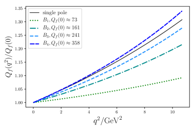
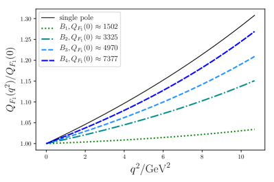
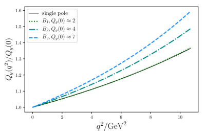
Figure 5: Comparison of the prefactor $Q_{F}(q^{2})$ for the BGL and BCL series expansions of form factor $F=f$, $F_{1}$, and $g$, from top to bottom. Curves are normalized by $Q_{F}(0)$, which is given in the legend.

The two functions in (37) are the outer functions $\phi_{F}(z)$, which can be found in the literature e.g. in Refs. Boyd:1997kz ; Bigi:2017njr ; Grinstein:2017nlq , and the Blaschke factor

$$B_{n}(z)=\prod_{i=1}^{n}\frac{z-z_{P_{i}}}{1-zz_{P_{i}}}\,,~{}~{}z_{P_{i}}=z(M_{P_{i}}^{2},t_{-})\,.$$ (39)

The product is over a set of applicable resonances, the vector $B_{c}^{*}$ states for $g$ and the axial vector $B_{c}$ states for $f$ and $F_{1}$. The resonances included in the Blaschke factor should be those with the appropriate quantum numbers and below scattering threshold. There are 4 $B_{c}$ vector and 4 axial-vector states conjectured to be below $BD^{*}$ threshold. Table 11 lists calculations of the vector and axial vector $B_{c}$ resonances. The model estimate for the mass of the heaviest vector state is very close to threshold, so has been left out of several analyses, including here. The magnitude of the Blaschke factors can be very sensitive to $n$, so leaving states out reduces the strength of unitarity constraints. This is illustrated in Fig. 5 for the $Q_{F}(q^{2})$ for $F=f$, $F_{1}$, and $g$.

Table 12: Results of $z$-expansion fits (36), either using the BGL (37) or BCL (40) parametrization. Unitarity constraints are not enforced in the fit, but the sums $S_{g}$ and $S_{fF}$ (38) are given for reference (see text). The number of $1^{+}/1^{-}$ resonances included in the Blaschke factor is $n_{B}^{+}/n_{B}^{-}$. Terms up to $O(z^{K-1})$ are included in the fits. Coefficients of higher order terms are consistent with zero.

fit	$n_{B}^{+}$	$n_{B}^{-}$	$K$	$I$	$a^{(f)}_{0}$	$a^{(f)}_{1}$	$a^{(F_{1})}_{0}$	$a^{(F_{1})}_{1}$	$a^{(g)}_{0}$	$a^{(g)}_{1}$	$S_{fF}$	$S_{g}$
BGL	2	2	2	0.0366(14)	$0.03005(39)$	$-0.120(51)$	$0.005031(65)$	$-0.0146(40)$	$0.032(15)$	$0.88(50)$	0.015(12)	0.78(89)
BGL	2	2	3	0.0376(16)	$0.03004(39)$	$-0.148(62)$	$0.005031(65)$	$-0.030(13)$	$0.029(14)$	$0.99(50)$	0.13(32)	0.98(98)
BGL	2	2	4	0.0376(16)	$0.03004(39)$	$-0.148(62)$	$0.005031(65)$	$-0.030(13)$	$0.029(14)$	$0.99(50)$	0.13(33)	0.98(98)
BGL	3	3	2	0.0368(15)	$0.01913(25)$	$-0.069(36)$	$0.003204(41)$	$-0.0073(27)$	$0.0138(85)$	$0.63(30)$	0.0052(49)	0.40(38)
BGL	3	3	3	0.0379(17)	$0.01913(25)$	$-0.088(47)$	$0.003204(41)$	$-0.0181(86)$	$0.0125(82)$	$0.68(31)$	0.06(21)	0.46(41)
BGL	3	3	4	0.0379(17)	$0.01913(25)$	$-0.088(47)$	$0.003204(41)$	$-0.0181(87)$	$0.0125(82)$	$0.68(31)$	0.06(22)	0.46(42)
BGL	4	3	2	0.0369(15)	$0.01228(16)$	$-0.035(24)$	$0.002057(26)$	$-0.0032(18)$	$0.0138(84)$	$0.63(30)$	0.0014(17)	0.39(38)
BGL	4	3	3	0.0380(17)	$0.01228(16)$	$-0.049(36)$	$0.002057(26)$	$-0.0102(57)$	$0.0129(86)$	$0.66(33)$	0.04(25)	0.44(43)
BGL	4	3	4	0.0380(17)	$0.01228(16)$	$-0.049(36)$	$0.002057(26)$	$-0.0102(59)$	$0.0129(85)$	$0.66(33)$	0.04(25)	0.44(42)
BCL	–	–	2	0.0367(15)	$0.01502(19)$	$-0.047(27)$	$0.002946(38)$	$-0.0029(27)$	$0.028(13)$	$0.78(44)$	0.0025(26)	0.60(69)
BCL	–	–	3	0.0378(17)	$0.01502(19)$	$-0.066(40)$	$0.002946(38)$	$-0.0136(82)$	$0.026(13)$	$0.82(46)$	0.08(38)	0.67(75)
BCL	–	–	4	0.0382(18)	$0.01502(19)$	$-0.311(42)$	$0.002946(38)$	$-0.0152(83)$	$0.109(16)$	$-0.29(38)$	0.144(67)	0.10(22)
BCL	–	–	5	0.0382(18)	$0.01502(19)$	$-0.311(42)$	$0.002946(38)$	$-0.0152(83)$	$0.109(16)$	$-0.29(38)$	0.144(67)	0.10(22)

Table 12 shows the results of BGL fits to the unfolded Belle data Abdesselam:2017kjf , varying the number of states included in the Blaschke factor and the number of terms kept in the $z$-expansion. The fits enforce the $q^{2}=0$ constraint on $F_{1}(0)$ and $f(0)$ at the $1\%$ level. Priors for the coefficients $a_{k}^{(F)}$ are Gaussians with mean 0 and standard deviation 1. Only the $k=0$ and 1 coefficients are tabulated; the others are not constrained by the data and remain statistically consistent with 0. As discussed above, the magnitude of these coefficients depends on the number of states in the Blaschke factor. Nevertheless, the results for $I$ are insensitive to this. On the other hand, $I$ does increase by about 0.001, or approximately $0.7\sigma$, when switching from $K=2$ to higher order polynomials in $z$. (Results remain the same for $K>4$.)

The fits presented in Table 12 do not enforce the unitarity bounds (38), but these bounds are not close to being saturated unless only two resonances are included in the Blaschke factors. Performing the fits with the bounds enforced did not significantly affect results. Considering the $n_{B}>2$, $K=4$ fits, increasing the standard deviation of the Gaussian priors for the series coefficients $a_{k}^{(F)}$ by a factor of 2 or 4 had very little effect on the parameters well-determined by the data, i.e. $I$, $a_{0}^{(f)}$, and $a_{0}^{(F_{1})}$, while the uncertainties in $a_{1}^{(f)}$, $a_{1}^{(F_{1})}$, $a_{0}^{(g)}$, $a_{1}^{(g)}$, $S_{fF}$, $S_{g}$, increased by factors of 1.5-2. For most of the $a_{k}^{(F)}$ with $k\geq 2$, the posterior distribution is the same as the prior, the exception being that $a_{2}^{(F_{1})}\lesssim 0.5$ seems preferred by the fit, even with wide prior widths.

To the extent that unitarity constraints do not affect the BGL fits, then a simpler approach would be to represent $Q_{F}(t)$ by a simple pole, as in the simplified series expansion (BCL) Bourrely:2008za . That is, one can parametrize the form factors by (36) with

$$Q_{F}(t)=\frac{N_{F}}{1-t/M_{P}^{2}}\,,$$ (40)

with $M_{P}$ being the mass of the lightest resonance with the appropriate quantum numbers. The normalization $N_{F}$ can be chosen so that the series coefficients are of the same order of magnitude as in a particular BGL expansion. With Fig. 5 as a guide, we take $N_{f}=300$, $N_{F_{1}}=7000$, and $N_{g}=5$. Once again we fit with priors for $a_{k}^{(F)}$ equal to $0\pm 1$. The results for $I$ show the same behaviour for the BCL fits as for the BGL fits.

The virtue of the BCL fit is in its simplicity. The BGL fit requires theory input for the outer functions $\phi_{F}$: perturbatively calculated derivatives of two-point functions at $q^{2}=0$ and $n_{I}$, the number of spectator quarks adjusted to account for $SU(3)_{F}$ breaking. (In the BGL fits here we take the values given in Table 2 of Ref. Bigi:2017njr .) The Blaschke factor requires as input model estimates for the excited $B_{c}$ resonances to include in the Blaschke factor. If unitarity bounds become tight enough to have an effect on the fits to data, then the effects of theoretical assumptions needs to be carefully included in the error analysis. On the other hand, the BCL fits only take as additional input the mass of a single resonance, available to very good precision from lattice QCD. In the future, fits to the BCL simplified $z$-expansion could provide a clean, benchmark fit.

Fig. 6 summarizes the consequences to $I$ of different fitting choices selected from Tables 10 and 12. The top two points show results from CLN fits including no uncertainties on the coefficients (34), or 10% errors on the $r_{h}$ coefficients and allowing the coefficients in the expansions of $R_{1,2}(w)$ to be $0\pm 1$. The bottom two points are respectively BGL and BCL fits with $K=4$, and $n_{B}^{+}=4$, $n_{B}^{-}=3$ for the BGL fit.

In Fig. 7 we compare the fit results, integrated over the experimental bins, of the tightly constrained CLN fit and the BGL and BCL fits (with $K=4$) to the Belle data Abdesselam:2017kjf . The agreement is generally good, with the notable exception of the $d\Gamma/dw$ in the smallest $w$ bin, where the CLN result is in greater tension with the data than the BGL and BCL results.

For the time being, with only one experimental data set available to carry out these investigations, determinations of $|V_{cb}|$ from $B\to D^{*}\ell\nu$ are less certain than has been thought. The BGL and BCL fits to Belle data indicate $I=0.038(2)$. Ref. Bailey:2014tva cites a private communication with C. Schwanda giving $\bar{\eta}_{EW}=\eta_{EW}\eta_{\mathrm{Coulomb}}=1.0182(16)$ as the product of the electroweak factor $\eta_{EW}=1.0066(16)$ and a term accounting for electromagnetic interactions between the charged $D^{*}$ and lepton in the final state. Combining this with the weighted average for $h_{A_{1}}\!(1)$ from Fermilab/MILC Bailey:2014tva and this work, we arrive at

$$|V_{cb}|=(41.3\pm 2.2)\times 10^{-3}$$ (41)

where the error is dominated by the experimental and related fitting uncertainty. This determination agrees well with both those from inclusive and exclusive $B\to D\ell\nu$ decays as shown in Fig. 8.

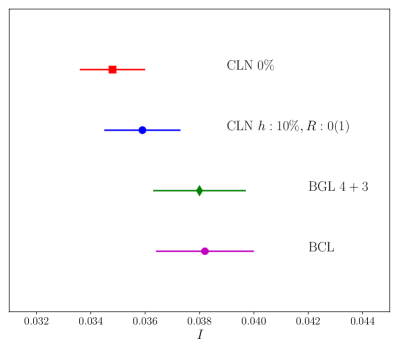
Figure 6: Values of $I=|\bar{\eta}_{EW}V_{cb}|h_{A_{1}}\!(1)$ obtained from different fit ansätze (see text).

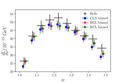
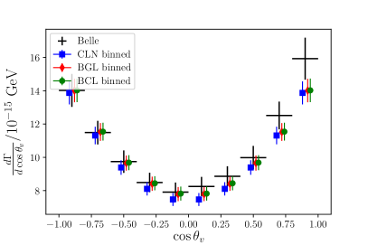
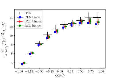
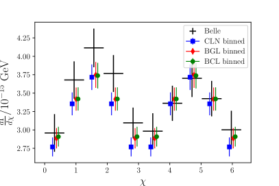
Figure 7: Comparison of fit results to experimental data Abdesselam:2017kjf . The binned fit results are slightly offset from the bin midpoints for clarity. See Appendix G and Ref. Abdesselam:2017kjf for definitions.

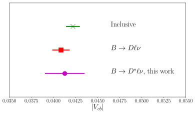
Figure 8: Comparison of the $|V_{cb}|$ from (41) with the latest determinations from $B\to X_{c}\ell\nu$ Bevan:2014iga ; Alberti:2014yda and $B\to D\ell\nu$ Aoki:2016frl .

One may ultimately obtain a more precise determination of $|V_{cb}|$ by including all relevant information, from HQET, by imposing stronger unitarity bounds Bigi:2017jbd , and including light cone sum rule calculations of form factors at large recoil Faller:2008tr . Comparison of the different approaches would be helpful to highlight the impact of including different ingredients.

VIII Conclusions

We present new unquenched lattice QCD determinations of the zero-recoil form factors $h_{A_{1}}\!(1)$ and $h_{A_{1}}^{s}\!(1)$, sometimes denoted $\mathcal{F}^{B\to D^{*}}(1)$ and $\mathcal{F}^{B_{s}\to D_{s}^{*}}(1)$, respectively. We have used 8 ensembles spanning 3 lattice spacings and 3 values of light-to-strange quark mass ratios, including the physical point. Our results are

$$\mathcal{F}^{B\to D^{*}}\!(1) =h_{A_{!}}\!(1)=0.895(10)_{\text{stat}}(24)_{\text{sys}}$$

$$\mathcal{F}^{B_{s}\to D_{s}^{*}}(1) =h^{s}_{A_{!}}\!(1)=0.883(12)_{\text{stat}}(28)_{\text{sys}}$$

$$\frac{\mathcal{F}^{B\to D^{*}}\!(1)}{\mathcal{F}^{B_{s}\to D_{s}^{*}}(1)} =\frac{h_{A_{1}}\!(1)}{h_{A_{1}}^{s}\!(1)}=1.013(14)_{\text{stat}}(17)_{\text{sys}}\,.$$ (42)

This result for $h_{A_{1}}\!(1)$ provides a valuable, independent check of the Fermilab/MILC result Bailey:2014tva . We have used completely independent sets of gauge field configurations and different formulations for the charm and bottom quarks. The two results are in good agreement.

While the determination of $|V_{cb}|$ using these results is complicated by the need to investigate assumptions used in extrapolating experimental data to zero recoil, series expansion fits to the unfolded Belle data yield

$$|V_{cb}|=(41.3\pm 2.2)\times 10^{-3}\,.$$ (43)

This is consistent with recent determinations using exclusive $B\to D\ell\nu$ and inclusive decays (Fig 8).

A reanalysis of BaBar data for the differential decay rate would complement the unfolded Belle data used here. We can also look forward to new data from Belle II, after which the the precision of $|V_{cb}|$ from $B\to D^{*}\ell\nu$ is likely to be much improved. Lattice QCD data away from zero recoil will also help reduce the uncertainties. Preliminary results from the Fermilab/MILC collaboration were presented at the Lattice 2017 conference Aviles-Casco:2017nge .

Our result for the $B_{s}\to D_{s}^{*}$ form factor is the first complete calculation of $h^{s}_{A_{1}}\!(1)$. In the future, measurements of the exclusive decays with a strange spectator, $B_{s}\to D_{s}^{(*)}\ell\nu$, could also provide a constraint on $|V_{cb}|$. LHCb has reconstructed $B_{s}^{0}\to D_{s}^{*-}\mu^{+}\nu_{\mu}$ decays Aaij:2017vqj . Eventually, with properly normalized branching fractions, these will also provide a method of constraining $|V_{cb}|$.

Spectator quark mass effects are bounded by our calculation of the ratio $h^{s}_{A_{1}}\!(1)/h_{A_{1}}\!(1)$ and its consistency with unity. We find deviations from $d\leftrightarrow s$ symmetry in the zero recoil $B_{(s)}\to D_{(s)}^{*}$ form factors to be no more than $2$-$3\%$.

Appendix A Gauge Action

The gauge action used to generate the configurations is the Symanzik and tadpole improved action of GaugeAction , which contains additional rectangle and parallelogram loops to cancel radiative $\mathcal{O}(a^{2})$ errors:

$$S= \sum_{x}\Big{[}a_{0}P_{0}(x)+a_{1}P_{1}(x)+a_{2}P_{2}(x)\Big{]}$$

$$P_{0}(x)= \sum_{\mu<\nu}U_{\mu\nu}(x)$$

$$P_{1}(x)= \sum_{\mu<\nu}U_{\mu\mu\nu}(x)+U_{\mu\nu\nu}(x)$$

$$P_{2}(x)= \sum_{\mu<\nu<\rho}U_{\mu\nu\rho}(x)+U_{\mu\rho\nu}(x)+U_{\rho\mu\nu}(x)+U_{\rho-\mu\nu}(x)$$

Where $-\mu$ indicates a Hermitian conjugated gauge link. $a_{1}$ and $a_{2}$ are calculated in terms of $a_{0}$ using lattice perturbation theory. The perturbative coefficients are specified in Ref. GaugeAction .

Appendix B $b$-Quarks Using NRQCD

In order to efficiently simulate the bottom quark we employ non-relativistic QCD (NRQCD) NRQCD . This formulation has been used for many calculations done by the HPQCD collaboration latticespacing ; PhysMasses ; Bmeson2 ; Bmeson ; Na:2015kha . The action is given in NRQCD , which we repeat here for clarity:

$$S=a^{3}\sum_{x}\Big{[} \psi^{\dagger}(x)\psi(x)-\psi(x+a\hat{t})\Big{(}1-\frac{aH_{0}}{2n}\Big{)}^{n}\Big{(}1-\frac{a\delta H}{2}\Big{)}$$

$$\times U^{\dagger}_{t}(x)\Big{(}1-\frac{a\delta H}{2}\Big{)}\Big{(}1-\frac{aH_{0}}{2n}\Big{)}^{n}\psi(x)\Big{]}\,.$$ (45)

The heavy quark propagator then satisfies the simple evolution equation

$$G(x+a\hat{t},z)= \delta(x+a\hat{t},z)+\Big{(}1-\frac{aH_{0}}{2n}\Big{)}^{n}\Big{(}1-\frac{a\delta H}{2}\Big{)}$$

$$\times U^{\dagger}_{t}(x)\Big{(}1-\frac{a\delta H}{2}\Big{)}\Big{(}1-\frac{aH_{0}}{2n}\Big{)}^{n}G(x,z)$$ (46)

with $G(x,y)=0$ for $x_{t}<y_{t}$, since the quark part of the action is first order in $D_{0}$ the propagator has no pole at $-E(p)$ and so is only the retarded part of the full propagator. This allows the bottom quark propagator to be computed by applying the evolution equation iteratively, allowing for faster, less memory intensive calculations and greater statistics.

The NRQCD quark action is tadpole improved OnLatticePT and Symanzik improved, with

$$aH_{0}= -\Delta^{(2)}/2am$$

$$a\delta H= -c_{1}\frac{(\Delta^{(2)})^{2}}{8(am)^{3}}+c_{2}\frac{ig}{8(am)^{2}}\big{(}\Delta\cdot\tilde{E}-\tilde{E}\cdot\Delta\big{)}$$

$$-c_{3}\frac{g}{8(am)^{2}}\sigma\cdot\big{(}\Delta\times\tilde{E}-\tilde{E}\times\Delta\big{)}$$

$$-c_{4}\frac{g}{2am}\sigma\cdot\tilde{B}+c_{5}\frac{a^{2}\Delta^{(4)}}{24am}-c_{6}\frac{a(\Delta^{(2)})^{2}}{16n(am)^{2}}$$ (47)

where the tilded quantities are the tadpole improved versions. In our simulations here we take the stability parameter $n=4$. The coefficients $c_{1}$-$c_{6}$ were computed perturbatively in latticespacing ; radcoefficients and are given in table II of Bmeson .

Appendix C HISQ Quarks

For the $u/d$ and $c$ valence quarks in our calculation we use the same HISQ action as for the sea quarks Follana:2006rc . The advantage of using HISQ is that $am_{q}$ discretization errors are under sufficient control that it can be used both for light and for $c$ quarks PrecDsupdate ; Follana:2006rc ; Follana:2007uv . The HISQ action is also numerically inexpensive as a result of the staggering which means we are able to attain better statistics. The valence $u/d$ masses are the same as those in the sea. The masses are given in Table 1. Below we summarize a few relevant facts.

The naive Dirac action has a discrete, space time dependent symmetry

$$\psi(x)\rightarrow\mathcal{B}_{\xi}(x)\psi(x)$$

$$\bar{\psi}(x)\rightarrow\bar{\psi}(x)\mathcal{B}^{\dagger}_{\xi}(x)$$ (48)

where

$$\mathcal{B}_{\xi}(x)=\gamma^{\bar{\xi}}(-1)^{\xi\cdot x}$$ (49)

and following Follana:2006rc

$$\gamma^{m}=\prod_{i=0}^{3}(\gamma^{i})^{m_{i}}$$

$$\overline{m}_{\mu}=\sum_{\eta\neq\mu}m_{\eta}\text{ mod 2}\,.$$ (50)

The conventions for $\gamma^{\bar{\xi}}$ are specified in the appendices. In momentum space this then gives the relation for the naive quark propagator:

$$S_{F}(p,q)=\mathcal{B}_{\xi}(0)S_{F}(p+\xi\pi,q+\xi\pi)\mathcal{B}_{\xi}(0)\,.$$ (51)

One can diagonalise the naive action in spin indices using a position dependent transformation of the fields. There are several choices for such a transformation, here we use:

$$\psi(x)\rightarrow\Omega(x)\chi(x)$$

$$\bar{\psi}(x)\rightarrow\bar{\chi}(x)\Omega^{\dagger}(x)$$ (52)

with $\Omega(x)=\gamma^{x}$ this yields the action

$$\mathcal{S}=\sum_{x,i}\bar{\chi}_{i}(x)(\alpha(x)\cdot\Delta(U)+m_{0})\chi_{i}(x)$$ (53)

with propagator

$$\langle\chi_{\kappa}(x)\bar{\chi}_{\delta}(y)\rangle=s(x,y)\delta_{\kappa\delta}\,.$$ (54)

We then need only do the inversion for a single component of $\chi$ and the full naive propagator can be reconstructed trivially by inserting $\Omega$ matrices:

$$S_{F}(x,y)_{\alpha\beta}= \langle\psi_{\alpha}(x)\bar{\psi}_{\beta}(y)\rangle=\Omega_{\alpha\kappa}(x)\langle\chi_{\kappa}(x)\bar{\chi}_{\delta}(y)\rangle\Omega^{\dagger}_{\delta\beta}(y)$$

$$= \Omega_{\alpha\delta}(x)\Omega^{\dagger}_{\delta\beta}(y)s(x,y)\,.$$ (55)

In order to remove discretization errors and taste exchange violations the operator $\Delta_{\mu}(U)$ used in simulations is more elaborate. It retains the feature that $\Delta_{\mu}(U)\psi(x)$ only contains fields $\psi(x^{\prime})$ located an odd number of lattice sites away from $x$ in the $\mu$ direction, ensuring that the spin-diagonalization $(12)$ still works. The full, highly improved staggered $SU(3)$-covariant derivative operator is Follana:2006rc :

$$\mathcal{D}^{\text{HISQ}}_{\mu}=\Delta_{\mu}(W)-\frac{a^{2}}{6}(1+\epsilon)\Delta^{3}_{\mu}(X)$$ (56)

with

$$W_{\mu} =\mathcal{F}^{\text{HISQ}}_{\mu}U_{\mu}$$

$$X_{\mu} =\mathcal{U}\mathcal{F}_{\mu}U_{\mu}$$

$$\mathcal{F}^{\text{HISQ}}_{\mu} =\left(\mathcal{F}_{\mu}-\sum_{\rho\neq\mu}\frac{a^{2}\delta_{\rho}^{2}}{2}\right)\mathcal{U}\mathcal{F}_{\mu}$$

$$\mathcal{F}_{\mu} =\prod_{\rho\neq\mu}\left(1+\frac{a^{2}\delta_{\rho}^{(2)}}{4}\right)_{\text{symm}}\,.$$ (57)

Where ‘symm’ indicates that the product ordering is symmetrised in $\rho$, $\delta_{\rho}$ approximates a covariant first derivative on the gauge links and $\delta^{(2)}_{\rho}$ approximates a second covariant derivative.

$$\delta_{\rho}U_{\mu}(x)= \frac{1}{a}\Big{(}U_{\rho}(x)U_{\mu}(x+a\hat{\rho})U^{\dagger}_{\rho}(x+a\hat{\mu})$$

$$-U^{\dagger}_{\rho}(x-a\hat{\rho})U_{\mu}(x-a\hat{\rho})U_{\rho}(x-a\hat{\rho}+a\hat{\mu})\Big{)}$$

$$\delta^{(2)}_{\rho}U_{\mu}(x) =\frac{1}{a^{2}}\Big{(}U_{\rho}(x)U_{\mu}(x+a\hat{\rho})U^{\dagger}_{\rho}(x+a\hat{\mu})$$

$$+U^{\dagger}_{\rho}(x-a\hat{\rho})U_{\mu}(x-a\hat{\rho})U_{\rho}(x-a\hat{\rho}+a\hat{\mu})$$

$$-2U_{\mu}(x)\Big{)}\,.$$ (58)

The third covariant derivative term removes order $a^{3}$ discretization errors coming from the approximation of the derivative. Without the epsilon term, tree level discretization errors appear going as $(ap_{\mu})^{4}$. For the mesons we are interested in quarks are typically nonrelativistic, and so the error is dominated by the energy, and ultimately the mass contribution going as $(am)^{4}$. For light quarks this is negligible, but for charm physics this must be included since current lattice spacings have $am_{c}\approx 0.5$. $\epsilon$ can be calculated straightforwardly as an expansion in $(am)^{2}$ by requiring the tree level dispersion relation $\lim_{p\rightarrow 0}{(E^{2}(p)-m^{2})}/{p^{2}}$ to have its correct value, $1$, to a given order $\mathcal{O}(am)$. The expansion is Follana:2006rc :

$$\epsilon=-\frac{27}{40}(am)^{2}+\frac{327}{1120}(am)^{4}-\frac{5843}{53760}(am)^{6}+\mathcal{O}((am)^{8})\,.$$ (59)

The smearings $\mathcal{F}_{\mu}$ remove taste changing interactions, since $\delta_{\rho}^{(2)}\approx-4/a^{2}$ when applied to a link carrying momentum $q_{\rho}\approx\pi/a$ The $\mu$ direction needn’t be smeared as the original interaction vanishes in this case anyway. The smearing $\mathcal{F}_{\mu}$, known as “Fat7” smearing fat7 , introduces new $\mathcal{O}(a^{2})$ errors. These are removed by replacing $\mathcal{F}_{\mu}$ with  ASQTAD

$$\mathcal{F}^{\text{ASQTAD}}_{\mu}=\mathcal{F}_{\mu}-\sum_{\rho\neq\mu}\frac{a^{2}\delta_{\rho}^{2}}{4}\,.$$ (60)

Where $\mathcal{F}^{\text{ASQTAD}}_{\mu}$ is the gauge link smearing employed in the widely used $a$-squared tadpole improved action. Similar errors originating from the smearing on the third derivative term needn’t be corrected as they go as $\mathcal{O}(a^{4})$. A single smearing introduces perpendicular gauge links which are themselves unsmeared. To further suppress taste exchange we use multiple smearings. Once such smearing is:

$$\mathcal{F}^{\text{ASQTAD}}_{\mu}\mathcal{U}\mathcal{F}^{\text{ASQTAD}}_{\mu}$$ (61)

where $\mathcal{U}$ is a reunitarization. This combination ensures that each smearing does not introduce any additional $\mathcal{O}(a^{2})$ errors, and ensures no growth in the size of two gluon vertices, since the unitarization ensures it is bounded by unity. In the HISQ operator defined in $(17)$ we have moved the entirety of the $\mathcal{O}(a^{2})$ corrections to the outermost smearing.

In order to check the taste exchange violations in HISQ one can check for taste-splittings of the pion masses. However since there are more allowed effective taste exchange vertices that there are degenerate pion multiplets this does not guarantee the theory is free of taste exchange. A better check is the explicit calculation of the couplings to taste exchange currents required to remove taste exchange. These are given in  Follana:2006rc in which it is clear that the HISQ action is a significant improvement over the older ASQTAD action.

Appendix D 3-point function

For real, symmetric, stride-2 smearings $\Delta$, suppressing Dirac indices for the moment, and summing over repeated indices and spatial coordinates for zero recoil:

$$C_{3pt}(x_{0},y_{0},z_{0})= \langle\bar{u}_{a}(x)M_{st}c_{a}(x+\sigma_{1}+\delta_{st})\bar{c}_{b}(y)\Gamma b_{b}(y)\bar{b}_{c}(z+\sigma_{2})\gamma u_{c}(z)\rangle\Delta_{1}(\sigma_{1})\Delta_{2}(\sigma_{2})$$

$$= \text{tr}\left[\Omega^{\dagger}(x)M_{st}\Omega(x+\delta_{st})S_{ab}^{c}(x+\sigma_{1}+\delta_{st},y)\Omega^{\dagger}(y)\Gamma\right]$$

$$\times\left[G_{bc}^{b}(y,z+\sigma_{2})\gamma\Omega(z)S_{ca}^{l}(z,x)\right]\Delta_{1}(\sigma_{1})\Delta_{2}(\sigma_{2})$$

$$= \text{tr}\left[\xi^{*}_{ea}(x)\Omega^{\dagger}(x)M_{st}\Omega(x+\delta_{st})S_{eb}^{c}(x+\sigma_{1}+\delta_{st},y)\Omega^{\dagger}(y)\Gamma\right]$$

$$\times\left[G_{bc}^{b}(y,z+\sigma_{2})\gamma\Omega(z)S_{cd}^{l}(z,x^{\prime})\xi_{da}(x^{\prime})\right]\Delta_{1}(\sigma_{1})\Delta_{2}(\sigma_{2})$$ (62)

where it is understood that when we add $\delta_{st}$ it is modulo the hypercube. We have used the noise condition:

$$\begin{split}\xi^{*}_{ab}(z)\xi_{cb}(y)=\delta_{ac}\delta_{xy}\end{split}$$ (63)

to insert the random walls. Setting

$$\text{Ext}_{ba}(y)=G_{bc}^{b}(y,z+\sigma_{2})\gamma\Omega(z)S_{cd}^{l}(z,x^{\prime})\xi_{da}(x^{\prime})\Delta_{2}(\sigma_{2})$$ (64)

this becomes

$$C_{3pt}(x_{0},y_{0},z_{0})= \text{tr}\left[\xi^{*}_{ea}(x)\Omega^{\dagger}(x)M_{st}\Omega(x+\delta_{st})S_{eb}^{c}(x+\sigma_{1}+\delta_{st},y)\Omega^{\dagger}(y)\Gamma\text{Ext}_{ba}(y)\right]\Delta_{1}(\sigma_{1})$$

$$= \text{tr}\left[\xi^{*}_{ea}(x-\sigma_{1})\Omega^{\dagger}(x)M_{st}\Omega(x+\delta_{st})S_{eb}^{c}(x+\delta_{st},y)\Omega^{\dagger}(y)\Gamma\text{Ext}_{ba}(y)\right]\Delta_{1}(\sigma_{1})\,.$$ (65)

Now, we do not have $S_{ab}^{c}(x,y)$, we have $S_{ab}^{c}(y,x)$ so we can use:

$$S^{*}_{ba}(x,y)=(-1)^{y}S_{ab}(y,x)(-1)^{x}$$ (66)

where $(-1)^{x}$ is shorthand for $(-1)^{x_{0}+x_{1}+x_{2}+x_{3}}$. Now

$$C_{3pt}(x_{0},y_{0},z_{0})= \text{tr}\left[\Omega^{\dagger}(y)(-1)^{y}S_{bc}^{c*}(y,x+\delta_{st})(-1)^{x+\delta_{st}}\beta_{M}(x)\xi^{*}_{ca}(x-\sigma_{1})\Gamma\text{Ext}_{ba}(y)\right]\Delta_{1}(\sigma_{1})$$ (67)

where $\beta_{M}(x)=\Omega^{\dagger}(x)M_{st}\Omega(x+\delta_{st})$ is the local spin-taste phase. Inserting Dirac indices:

$$C_{3pt}(x_{0},y_{0},z_{0})= \Omega^{\dagger}_{\alpha\beta}(y)(-1)^{y}S_{bc}^{c*}(y,x)(-1)^{x}\beta_{M}(x+\delta_{st})\xi^{*}_{ca}(x-\sigma_{1}+\delta_{st})\Delta_{1}(\sigma_{1})\Gamma_{\beta\kappa}\text{Ext}_{ba,\kappa\alpha}(y)$$

$$= \pm\left[\Omega_{\beta\alpha}(y)(-1)^{y}S_{bc}^{c}(y,x)(-1)^{x}\beta_{M}(x)\xi_{ca}(x-\sigma_{1}+\delta_{st})\Delta_{1}(\sigma_{1})\right]^{*}\Gamma_{\beta\kappa}\text{Ext}_{ba,\kappa\alpha}(y)\,.$$ (68)

We recognise $S_{bc}^{c}(y,x)(-1)^{x}\beta_{M}(x)\xi_{ca}(x-\sigma_{1}+\delta_{st})\Delta_{1}(\sigma_{1})$ as the MILC KS propagator. The naive active quark that gets made in NRQCD is then:

$$\text{Active}_{ab,\alpha\beta}(y)=\Omega_{\alpha\beta}(y)(-1)^{y}S_{ac}^{c}(y,x)(-1)^{x}\beta_{M}(x)\xi_{cb}(x-\sigma_{1}+\delta_{st})\Delta_{1}(\sigma_{1})$$ (69)

and the contractions to do are

$$\text{Current}_{ab,\alpha\beta}(y)=\text{Active}^{*}_{ba,\kappa\alpha}(y)\Gamma_{\kappa\beta}$$

$$C_{3pt}=\text{Current}_{ab,\alpha\beta}(y)\text{Ext}_{ba,\beta\alpha}(y)\,.$$ (70)

Appendix E Correlator Fits

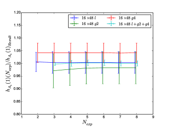
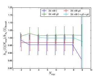
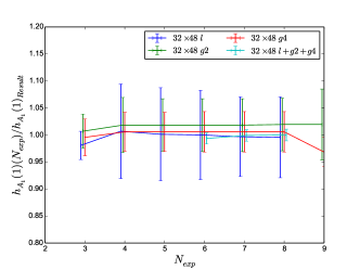
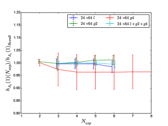
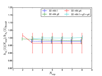
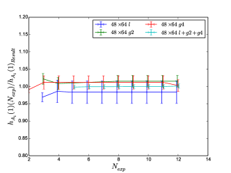
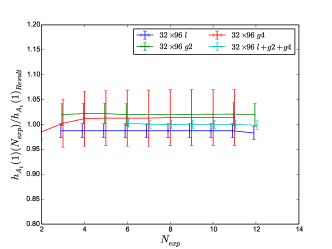
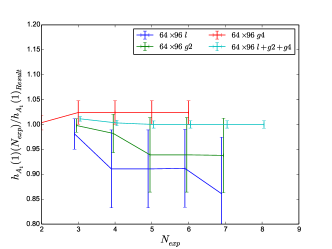
Figure 9: Plots of $N_{\text{exp}}$ fit behaviour on all 8 ensembles (see Tab. 1). In each plot 4 sets of data points are shown: the full fit including all $3\times 3$ source-sink combinations, and, for comparison, separate “diagonal” fits where only one type of source-sink smearing is used. (The notation is defined in Sec. III.) A significant improvement is seen in the full fit. All diagonal fits show good agreement for $N_{\text{exp}}\geq 4$, but with the increased precision, sometimes 5 or 6 exponentials are needed to get a good $3\times 3$ matrix fit.

Fig. 9 shows comparison of the fit results for $h_{A_{1}}\!(1)$ when varying numbers of exponentials; the points are normalized by the value of taken $h_{A_{1}}\!(1)$ as our result for that ensemble. Plots are shown for all 8 ensembles as listed in Tab. 1. In each plot, we show the full fit results to the $3\times 3$ matrix of source/sink combinations (local $l$, or Gaussian with 2 radii, $g2$ and $g4$), as well as “diagonal” fits where only one source/sink is used. The statistical improvement of using all the data is apparent. The flatness of the curves and the constancy of the error bars shows that, for large enough $N_{\mathrm{exp}}$, the Bayesian fits are insensitive to adding further exponential terms, i.e. effects of excited states are accounted for. Our final results typically come from the $N_{\mathrm{exp}}=5$ fits to the full $3\times 3$ matrix of correlators; however, on ensembles 3 and 7, we had to include another exponential.

Appendix F Chiral continuum fit function

The full expression for the form factor derived in staggered chiral perturbation theory is given by SCHIPT

$$h_{A_{1}}\!(1)=1+\frac{X(\Lambda_{\chi})}{m_{c}^{2}}+\frac{g_{\pi}^{2}}{48\pi^{2}f^{2}}\Big{[}\frac{1}{16}\sum_{\delta}(2\bar{F}_{\pi_{\delta}}+\bar{F}_{K_{\delta}})-\frac{1}{2}\bar{F}_{\pi_{I}}+\frac{1}{6}\bar{F}_{\eta_{I}}$$

$$+a^{2}\delta^{\prime}_{V}\Big{(}\frac{m_{S_{V}}^{2}-m_{\pi_{V}}^{2}}{(m_{\eta_{V}}^{2}-m_{\pi_{V}}^{2})(m_{\pi_{V}}^{2}-m_{\eta^{\prime}_{V}}^{2})}\bar{F}_{\pi_{V}}+\frac{m_{\eta_{V}}^{2}-m_{S_{V}}^{2}}{(m_{\eta_{V}}^{2}-m_{\eta^{\prime}_{V}}^{2})(m_{\eta_{V}}^{2}-m_{\pi_{V}}^{2})}\bar{F}_{\eta_{V}}$$

$$+\frac{m_{S_{V}}^{2}-m_{\eta^{\prime}_{V}}^{2}}{(m_{\eta_{V}}^{2}-m_{\eta^{\prime}_{V}}^{2})(m_{\eta^{\prime}_{V}}^{2}-m_{\pi_{V}}^{2})}\bar{F}_{\eta^{\prime}_{V}}\Big{)}+(V\rightarrow A)\Big{]}$$ (71)

where $\bar{F}_{X}=F[m_{X},-\Delta_{m_{c}}/m_{X}]$ and

$$F[m,x]= \frac{m^{2}}{x}\Big{\{}x^{3}\ln\frac{m^{2}}{\Lambda_{\chi}^{2}}+\frac{1}{3}x^{3}-4x+2\pi$$

$$-\sqrt{x^{2}-1}(x^{2}+2)$$

$$\times\big{(}\ln\big{[}1-2x(x-\sqrt{x^{2}-1})\big{]}-i\pi\big{)}\Big{\}}\,.$$ (72)

The masses of the $\eta$ and $\eta^{\prime}$ are given in staggeredmasses as

$$m_{\eta_{V}}^{2} =\frac{1}{2}\left(m_{\pi_{V}}^{2}+m_{S_{V}}^{2}+\frac{3}{4}a^{2}\delta^{\prime}_{V}-Z\right)$$

$$m_{\eta^{\prime}_{V}}^{2} =\frac{1}{2}\left(m_{\pi_{V}}^{2}+m_{S_{V}}^{2}+\frac{3}{4}a^{2}\delta^{\prime}_{V}+Z\right)$$

$$Z =\sqrt{(m_{S_{V}}^{2}-m_{\pi_{V}}^{2})^{2}-\frac{a^{2}\delta^{\prime}_{V}}{2}(m_{S_{V}}^{2}-m_{\pi_{V}}^{2})+\frac{9(a^{2}\delta^{\prime}_{V})^{2}}{16}}$$

$$=(m_{S_{V}}^{2}-m_{\pi_{V}}^{2})-\frac{a^{2}\delta^{\prime}_{V}}{4}+\mathcal{O}((a^{2}\delta^{\prime}_{V})^{2})$$

$$m_{\eta_{I}}^{2} =m_{\pi_{I}}^{2}/3+2m_{S_{I}}^{2}/3\,.$$ (73)

We take the $s\bar{s}$ pseudoscalar taste splittings equal to the pion taste splittings. This is a good approximation in the case of HISQ Bazavov:2012xda . We can then write (to order $\mathcal{O}((a^{2}\delta^{\prime}_{V})^{2})$ )

$$m_{\eta^{\prime}_{V}}^{2}-m_{\pi_{V}}^{2}= m_{S_{G}}^{2}-m_{\pi_{G}}^{2}+a^{2}\delta^{\prime}_{V}/4$$

$$m_{\eta_{V}}^{2}-m_{\pi_{V}}^{2}= a^{2}\delta^{\prime}_{V}/2$$

$$m_{S_{V}}^{2}-m_{\pi_{V}}^{2}= m_{S_{G}}^{2}-m_{\pi_{G}}^{2}$$ (74)

from which we find

$$\frac{m_{S_{V}}^{2}-m_{\eta^{\prime}_{V}}^{2}}{(m_{\eta_{V}}^{2}-m_{\eta^{\prime}_{V}}^{2})(m_{\eta^{\prime}_{V}}^{2}-m_{\pi_{V}}^{2})} =\frac{a^{2}\delta^{\prime}_{V}/4}{(m_{S_{G}}^{2}-m_{\pi_{G}}^{2})^{2}-(a^{2}\delta^{\prime}_{V}/4)^{2}}$$

$$\frac{m_{\eta_{V}}^{2}-m_{S_{V}}^{2}}{(m_{\eta_{V}}^{2}-m_{\eta^{\prime}_{V}}^{2})(m_{\eta_{V}}^{2}-m_{\pi_{V}}^{2})} =\frac{a^{2}\delta^{\prime}_{V}/2-(m_{S_{G}}^{2}-m_{\pi_{G}}^{2})}{(a^{2}\delta^{\prime}_{V}/4-(m_{S_{G}}^{2}-m_{\pi_{G}}^{2}))a^{2}\delta^{\prime}_{V}/2}$$

$$\frac{m_{S_{V}}^{2}-m_{\pi_{V}}^{2}}{(m_{\eta_{V}}^{2}-m_{\pi_{V}}^{2})(m_{\pi_{V}}^{2}-m_{\eta^{\prime}_{V}}^{2})} =\frac{-(m_{S_{G}}^{2}-m_{\pi_{G}}^{2})}{((m_{S_{G}}^{2}-m_{\pi_{G}}^{2})-a^{2}\delta^{\prime}_{V}/4)a^{2}\delta^{\prime}_{V}/2}\,.$$ (75)

The expression for $h_{A_{1}}\!(1)$ then reduces to

$$h_{A_{1}}\!(1)=1+\frac{X(\Lambda_{\chi})}{m_{c}^{2}}+ \frac{g_{\pi}^{2}}{48\pi^{2}f^{2}}\Bigg{[}\frac{1}{16}\sum_{\delta}2\bar{F}_{\pi_{\delta}}-\frac{1}{2}\bar{F}_{\pi_{I}}+\left(2-\frac{a^{2}\delta^{\prime}_{V}}{2(m_{S_{G}}^{2}-m_{\pi_{G}}^{2})}\right)\bar{F}_{\eta_{V}}+\left(2-\frac{a^{2}\delta^{\prime}_{A}}{2(m_{S_{G}}^{2}-m_{\pi_{G}}^{2})}\right)\bar{F}_{\eta_{A}}$$

$$- \left(2+\frac{a^{2}\delta^{\prime}_{V}}{2(m_{S_{G}}^{2}-m_{\pi_{G}}^{2})}\right)\bar{F}_{\pi_{V}}-\left(2+\frac{a^{2}\delta^{\prime}_{A}}{2(m_{S_{G}}^{2}-m_{\pi_{G}}^{2})}\right)\bar{F}_{\pi_{A}}\Bigg{]}+\mathcal{O}((a^{2}\delta^{\prime}_{V})^{2})$$ (76)

where we have ignored terms expected to produce normal discretization errors and pion mass dependence, as these are included elsewhere in the fit. Following PIMASSES we take $\delta A^{\prime}\approx\delta V^{\prime}\approx-\delta t$, which we implement by including $\delta A^{\prime}=\delta V^{\prime}=-\delta t\times 1.0(5)$ as priors. We use the pion masses computed in PIMASSES together with the taste splittings for the pion, $\delta t$, given in Bazavov:2012xda .

Finite volume effects can be accounted for in heavy meson chiral perturbation theory Arndt:2004bg including taste-splitting effects in the staggered pions SCHIPT . The functions $\bar{F}_{X}$ in (76) receive a correction term corresponding to the difference between infinite volume loop integrals and finite volume discrete sums. Taste-splitting effects in the pions at non-zero lattice spacing moderate the size of the finite volume corrections because some of the pions in the loops have heavier masses than the Goldstone pion. Consequently, some of the finite volume effect appears as a lattice-spacing effect, which is dealt with by our chiral-continuum fit.

We incorporated the finite volume corrections into our fit by subtracting from our data $\delta_{FV}h_{A_{1}}(1)$, found by adding $\delta\bar{F}_{X}$ to each $\bar{F}_{X}$ appearing in (76). In Fig. 10 we show $\delta_{FV}h_{A_{1}}(1)$ as a function of pion mass for the parameters appropriate for the physical pion mass lattices, Sets 3, 6, and 8 (see Table 1). For the other lattices, $|\delta_{FV}h_{A_{1}}(1)|\approx O(0.1\%)$ over the $M_{\pi}$ range where we have data and is not significant.

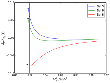
Figure 10: Pion mass dependence of the finite volume corrections to $h_{A_{1}}(1)$, as determined from staggered chiral perturbation theory SCHIPT , with parameters corresponding to the physical-mass lattices used here. The curves for the heavier-mass lattices used here show much smaller finite volume corrections, of $O(0.1\%)$. The vertical blue line is the physical pion mass and the solid point at the end of each curve is at the measured value of the pion mass on each lattice.

In Table 13 we give fit results for plausible variations on our chosen fit function as a demonstration of stability under such nontrivial choices. Neglecting different powers of $a^{2}$ we see that our result is only sensitive to leading $\mathcal{O}(a^{2})$ errors. The $M_{\pi}^{2}$ dependence we included does not affect the central value if removed, nor do changes in the assumed correlations between NRQCD systematics between ensembles. Removing taste splitting terms in the chiral perturbation theory result down to the continuum formula results in only a small change to the central value. Adding $\alpha_{s}\Lambda_{{\scriptscriptstyle\mathrm{QCD}}}/M_{B}$, which we have excluded from our fit due to Luke’s theorem, results in a slight increase in the central value as well as the expected increase in error. Our result is also only mildly sensitive to different choices of $\Lambda_{{\scriptscriptstyle\mathrm{QCD}}}$ which we vary by $\pm 50\%$. Taken collectively we note that no tested variations result in more than a $0.25\sigma$ change to the central value.

Table 13: Fit results for $h_{A_{1}}\!(1)$ for different chiral-continuum fit functions

Fit function	$h_{A_{1}}\!(1)$	$h^{s}_{A_{1}}\!(1)$
Eq. (76)	0.895(26)	0.883(31)
excluding hairpin terms	0.895(26)	0.883(31)
continuum $\chi PT$ formula	0.897(25)	0.882(31)
$\Lambda_{{\scriptscriptstyle\mathrm{QCD}}}=750$ MeV	0.900(35)	0.882(38)
$\Lambda_{{\scriptscriptstyle\mathrm{QCD}}}=250$ MeV	0.897(24)	0.890(23)
excluding polynomial $\mathcal{O}(a^{6})$ terms	0.895(26)	0.883(31)
excluding polynomial $\mathcal{O}(a^{4})$ terms	0.895(26)	0.883(31)
excluding polynomial $\mathcal{O}(a^{2})$ terms	0.898(26)	0.891(25)
excluding polynomial $M_{\pi}^{2}$ dependence	0.895(27)	0.883(31)
excluding $(\Lambda/M_{B})^{2}$ uncertainty	0.895(25)	0.883(31)
totally correlated $(\Lambda_{{\scriptscriptstyle\mathrm{QCD}}}/M_{B})^{2}$ errors	0.895(27)	0.883(31)

Appendix G Fits to Experimental Data

The fully differential decay rate is given by Richman:1995wm ; Abdesselam:2017kjf

$$\frac{d\Gamma(\bar{B}\to D^{*}\ell\,\bar{\nu}_{\ell})}{dw\,d\cos\theta_{v}\,d\cos\theta_{\ell}\,d\chi}=\frac{3G_{F}^{2}\left|\bar{\eta}_{EW}V_{cb}\right|^{2}}{1024\pi^{4}}\frac{M_{D^{*}}^{2}}{M_{B}}q^{2}\,\sqrt{w^{2}-1}$$

$$~{}~{}\times\Big{[}(1-\cos\theta_{\ell})^{2}\sin^{2}\theta_{v}H_{+}^{2}+(1+\cos\theta_{\ell})^{2}\sin^{2}\theta_{v}H_{-}^{2}$$

$$~{}~{}+4\sin^{2}\theta_{\ell}\cos^{2}\theta_{v}H_{0}^{2}-2\sin^{2}\theta_{\ell}\sin^{2}\theta_{v}\cos 2\chi H_{+}H_{-}$$

$$~{}~{}-4\sin\theta_{\ell}(1-\cos\theta_{\ell})\sin\theta_{v}\cos\theta_{v}\cos\chi H_{+}H_{0}$$

$$~{}~{}+4\sin\theta_{\ell}(1+\cos\theta_{\ell})\sin\theta_{v}\cos\theta_{v}\cos\chi H_{-}H_{0}\Big{]}$$ (77)

where $H_{+}(w)$, $H_{-}(w)$, and $H_{0}(w)$ are helicity amplitudes. In principle these amplitudes could be determined from lattice QCD, but presently these must be parametrized and fit to experiment, with a lattice calculation of the zero recoil form factor providing the normalization. Integrating (77) over the angular variables gives Eq. (1), with

$$\chi(w)|\mathcal{F}(w)|^{2}=\frac{r(1-2wr+r^{2})}{12M_{B}^{2}(1-r)^{2}}\sum_{i=\pm,0}|H_{i}|^{2}\,.$$ (78)

with $r=M_{D^{*}}/M_{B}$. Although not necessary in this work, it is conventional to factor out the kinematic function

$$\chi(w)=\frac{(w+1)^{2}}{12}\left[1+\frac{4w}{w+1}\frac{1-2wr+r^{2}}{(1-r)^{2}}\right]\,.$$ (79)

Note that $\chi(1)=1$ here, although different normalizations appear in the literature.

The CLN parametrization expresses the helicity amplitudes as follows Caprini:1997mu ; Neubert:1993mb . The reduced helicity amplitudes $\tilde{H}_{i}$ are defined by

$$H_{i}(w)=(M_{B}-M_{D^{*}})(1+w)\sqrt{\frac{M_{B}\,M_{D^{*}}}{q^{2}}}\,h_{A_{1}}\!(w)\,\tilde{H}_{i}(w)\,.$$ (80)

Then

$$\tilde{H}_{\pm}(w) =\frac{\sqrt{1-2wr+r^{2}}}{1-r}\left[1\mp\sqrt{\frac{w-1}{w+1}}\,R_{1}(w)\right]$$

$$\tilde{H}_{0}(w) =1+\frac{w-1}{1-r}[1-R_{2}(w)]\,$$ (81)

where $r=M_{D^{*}}/M_{B}$. The $h_{A_{1}}\!(w)$, $R_{1}(w)$, $R_{2}(w)$ then expanded in $z$ or $w-1$, as given in (33).

In the BGL parametrization Boyd:1997kz (and in the simplified BCL parametrization we employ) the helicity amplitudes are written in terms of the $f$, $F_{1}$, and $g$ form factors as follows

$$H_{\pm}(w) =f(z)\mp M_{B}\,M_{D^{*}}\sqrt{w^{2}-1}\,g(z)$$

$$H_{0}(w) =\frac{F_{1}(z)}{\sqrt{q^{2}}}\,.$$ (82)

These form factors are then expressed as in (36).

References

- (1) H. Albrecht et al. (ARGUS Collaboration), Phys. Lett. B 197, 452 (1987).
- (2) D. Bortoletto et al. (CLEO Collaboration), Phys. Rev. Lett. 63, 1667 (1989).
- (3) R. Fulton et al. (CLEO Collaboration), Phys. Rev. D 43, 651 (1991).
- (4) H. Albrecht et al. (ARGUS Collaboration), Phys. Lett. B 275, 195 (1992).
- (5) B. Barish et al. (CLEO Collaboration), Phys. Rev. D 51, 1014 (1995), arXiv:hep-ex/9406005.
- (6) D. Buskulic et al. (ALEPH Collaboration), Phys. Lett. B 359, 236 (1995).
- (7) D. Buskulic et al. (ALEPH Collaboration), Phys. Lett. B 395, 373 (1997).
- (8) G. Abbiendi et al. (OPAL Collaboration), Phys. Lett. B 482, 15 (2000), arXiv:hep-ex/0003013.
- (9) P. Abreu et al. (DELPHI Collaboration), Phys. Lett. B 510, 55 (2001), arXiv:hep-ex/0104026.
- (10) N. E. Adam et al. (CLEO Collaboration), Phys. Rev. D 67, 032001 (2003), arXiv:hep-ex/0210040.
- (11) J. Abdallah et al. (DELPHI Collaboration), Eur. Phys. J. C 33, 213 (2004), arXiv:hep-ex/0401023.
- (12) B. Aubert et al. (BaBar Collaboration), Phys. Rev. D 77, 032002 (2008), arXiv:0705.4008.
- (13) B. Aubert et al. (BaBar Collaboration), Phys. Rev. Lett. 100, 231803 (2008), arXiv:0712.3493.
- (14) B. Aubert et al. (BaBar Collaboration), Phys. Rev. D 79, 012002 (2009), arXiv:0809.0828.
- (15) W. Dungel et al. (Belle Collaboration), Phys. Rev. D 82, 112007 (2010), arXiv:1010.5620.
- (16) A. Abdesselam et al. (Belle Collaboration), (2017), arXiv:1702.01521.
- (17) Y. Amhis et al. (HFLAV Collaboration), (2016), arXiv:1612.07233.
- (18) J. A. Bailey et al., Phys. Rev. D 89, 114504 (2014), arXiv:1403.0635.
- (19) A. J. Bevan et al., Eur. Phys. J. C 74, 3026 (2014), arXiv:1406.6311.
- (20) A. Alberti, P. Gambino, K. J. Healey, and S. Nandi, Phys. Rev. Lett. 114, 061802 (2015), arXiv:1411.6560.
- (21) I. Caprini, L. Lellouch, and M. Neubert, Nucl. Phys. B 530, 153 (1998), arXiv:hep-ph/9712417.
- (22) F. U. Bernlochner, Z. Ligeti, M. Papucci, and D. J. Robinson, Phys. Rev. D 95, 115008 (2017), arXiv:1703.05330.
- (23) D. Bigi, P. Gambino, and S. Schacht, Phys. Lett. B 769, 441 (2017), arXiv:1703.06124.
- (24) B. Grinstein and A. Kobach, Phys. Lett. B 771, 359 (2017), arXiv:1703.08170.
- (25) D. Bigi, P. Gambino, and S. Schacht, (2017), arXiv:1707.09509.
- (26) S. Jaiswal, S. Nandi, and S. K. Patra, (2017), arXiv:1707.09977.
- (27) F. U. Bernlochner, Z. Ligeti, M. Papucci, and D. J. Robinson, (2017), arXiv:1708.07134.
- (28) C. G. Boyd, B. Grinstein, and R. F. Lebed, Phys. Rev. D 56, 6895 (1997), arXiv:hep-ph/9705252.
- (29) J. A. Bailey et al., Phys. Rev. D 92, 034506 (2015), arXiv:1503.07237.
- (30) H. Na et al., Phys. Rev. D 92, 054510 (2015), arXiv:1505.03925, [Erratum: Phys. Rev. D 93, 119906 (2016)].
- (31) C. G. Boyd, B. Grinstein, and R. F. Lebed, Phys. Rev. Lett. 74, 4603 (1995), arXiv:hep-ph/9412324.
- (32) C. Bourrely, L. Lellouch, and I. Caprini, Phys. Rev. D 79, 013008 (2009), arXiv:0807.2722.
- (33) S. Aoki et al. (FLAG Collaboration), Eur. Phys. J. C 77, 112 (2017), arXiv:1607.00299.
- (34) A. J. Buras and D. Guadagnoli, Phys. Rev. D 78, 033005 (2008), arXiv:0805.3887.
- (35) A. Bazavov et al. (MILC Collaboration), Phys. Rev. D 82, 074501 (2010), arXiv:1004.0342.
- (36) A. Bazavov et al. (MILC Collaboration), Phys. Rev. D 87, 054505 (2013), arXiv:1212.4768.
- (37) A. Bazavov et al. (MILC Collaboration), Phys. Rev. D 93, 094510 (2016), arXiv:1503.02769.
- (38) E. Follana et al. (HPQCD Collaboration), Phys. Rev. D 75, 054502 (2007), arXiv:hep-lat/0610092.
- (39) G. P. Lepage, L. Magnea, C. Nakhleh, U. Magnea, and K. Hornbostel, Phys. Rev. D 46, 4052 (1992), hep-lat/9205007.
- (40) J. Harrison, C. Davies, and M. Wingate, Proc. Sci. LATTICE2016, 287 (2016), arXiv:1612.06716.
- (41) M. Atoui, V. Morénas, D. Bečirević, and F. Sanfilippo, Eur. Phys. J. C 74, 2861 (2014), arXiv:1310.5238.
- (42) J. Flynn et al., Proc. Sci. LATTICE2016, 296 (2016), arXiv:1612.05112.
- (43) A. Sirlin, Nucl. Phys. B 196, 83 (1982).
- (44) E. S. Ginsberg, Phys. Rev. 171, 1675 (1968), [Erratum: Phys. Rev. 174, 2169 (1968)].
- (45) D. Atwood and W. J. Marciano, Phys. Rev. D 41, 1736 (1990).
- (46) R. J. Dowdall et al. (HPQCD Collaboration), Phys. Rev. D 85, 054509 (2012), arXiv:1110.6887.
- (47) B. Chakraborty et al. (HPQCD Collaboration), Phys. Rev. D 91, 054508 (2015), arXiv:1408.4169.
- (48) A. Bazavov et al. (Fermilab Lattice and MILC Collaborations), Phys. Rev. D 90, 074509 (2014), arXiv:1407.3772.
- (49) A. Hart, G. M. von Hippel, and R. R. Horgan, Phys. Rev. D 79, 074008 (2009), arXiv:0812.0503.
- (50) MILC Code Repository, https://github.com/milc-qcd.
- (51) G. P. Lepage, L. Magnea, C. Nakhleh, U. Magnea, and K. Hornbostel, Phys. Rev. D 46, 4052 (1992), arXiv:hep-lat/9205007.
- (52) J. J. Dudek, R. G. Edwards, and D. G. Richards, Phys. Rev. D 73, 074507 (2006), arXiv:hep-ph/0601137.
- (53) C. Monahan, J. Shigemitsu, and R. Horgan, Phys. Rev. D 87, 034017 (2013), arXiv:1211.6966.
- (54) C. J. Morningstar and J. Shigemitsu, Phys. Rev. D 59, 094504 (1999), arXiv:hep-lat/9810047.
- (55) M. E. Luke, Phys. Lett. B 252, 447 (1990).
- (56) C. McNeile, C. T. H. Davies, E. Follana, K. Hornbostel, and G. P. Lepage (HPQCD Collaboration), Phys. Rev. D 82, 034512 (2010), arXiv:1004.4285.
- (57) G. P. Lepage et al., Nucl. Phys. Proc. Suppl. 106, 12 (2002), hep-lat/0110175.
- (58) G.P. Lepage, Corrfitter Version 4.1, github.com/gplepage/corrfitter.git.
- (59) B. Colquhoun et al., Phys. Rev. D 91, 114509 (2015), arXiv:1503.05762.
- (60) J. Laiho, R.S. Van de Water, Phys. Rev. D 73, 054501 (2006), arXiv:hep-lat/0512007.
- (61) R. J. Dowdall, C. T. H. Davies, R. R. Horgan, C. J. Monahan, and J. Shigemitsu, Phys. Rev. Lett. 110, 222003 (2013), arXiv:1302.2644.
- (62) B. Colquhoun, C. Davies, J. Koponen, A. Lytle, and C. McNeile (HPQCD Collaboration), PoS LATTICE2016, 281 (2016), arXiv:1611.01987.
- (63) R. Dowdall, C. Davies, T. Hammant, and R. Horgan, Phys. Rev. D 86, 094510 (2012), arXiv:1207.5149.
- (64) C. Patrignani et al. (PDG Collaboration), Chin. Phys. C 40, 100001 (2016).
- (65) N. Devlani, V. Kher, and A. K. Rai, Eur. Phys. J. A 50, 154 (2014).
- (66) S. Godfrey, Phys. Rev. D 70, 054017 (2004), arXiv:hep-ph/0406228.
- (67) E. J. Eichten and C. Quigg, Phys. Rev. D 49, 5845 (1994), arXiv:hep-ph/9402210.
- (68) S. Faller, A. Khodjamirian, C. Klein, and T. Mannel, Eur. Phys. J. C 60, 603 (2009), arXiv:0809.0222.
- (69) A. Vaquero Avilés-Casco et al., (2017), arXiv:1710.09817.
- (70) R. Aaij et al. (LHCb Collaboration), (2017), arXiv:1705.03475.
- (71) G. P. Lepage and P. B. Mackenzie, Phys. Rev. D 48, 2250 (1993), arXiv:hep-lat/9209022.
- (72) T. Hammant, A. Hart, G. von Hippel, R. Horgan, and C. Monahan, Phys. Rev. Lett. 107, 112002 (2011), arXiv:1105.5309.
- (73) C. T. H. Davies et al., Phys. Rev. D 82, 114504 (2010), arXiv:1008.4018.
- (74) E. Follana, C. T. H. Davies, G. P. Lepage, and J. Shigemitsu, Phys. Rev. Lett. 100, 062002 (2008), arXiv:0706.1726.
- (75) D. Toussaint and K. Orginos, Nucl. Phys. Proc. Suppl. 73, 909 (1999), hep-lat/9809148.
- (76) G. P. Lepage, Phys. Rev. D 59, 074502 (1999), arXiv:hep-lat/9809157.
- (77) C. Aubin and C. Bernard, Phys. Rev. D 68, 034014 (2003), arXiv:hep-lat/0304014.
- (78) R. J. Dowdall, C. T. H. Davies, G. P. Lepage, and C. McNeile, Phys. Rev. D 88, 074504 (2013), arXiv:1303.1670.
- (79) D. Arndt and C. J. D. Lin, Phys. Rev. D 70, 014503 (2004), arXiv:hep-lat/0403012.
- (80) J. D. Richman and P. R. Burchat, Rev. Mod. Phys. 67, 893 (1995), arXiv:hep-ph/9508250.
- (81) M. Neubert, Phys. Rept. 245, 259 (1994), arXiv:hep-ph/9306320.