Leader-based Optimal Coordination Control for the Consensus Problem of Multi-agent Differential Games via Fuzzy Adaptive Dynamic Programming

Abstract

In this paper, a new online scheme is presented to design the optimal coordination control for the consensus problem of multi-agent differential games by fuzzy adaptive dynamic programming (FADP), which brings together game theory, generalized fuzzy hyperbolic model (GFHM) and adaptive dynamic programming (ADP). In general, the optimal coordination control for multi-agent differential games is the solution of the coupled Hamilton-Jacobi (HJ) equations. Here, for the first time, GFHMs are used to approximate the solutions (value functions) of the coupled HJ equations, based on policy iteration (PI) algorithm. Namely, for each agent, GFHM is used to capture the mapping between the local consensus error and local value function. Since our scheme uses the single-network architecture for each agent (which eliminates the action network model compared with dual-network architecture), it is a more reasonable architecture for multi-agent systems. Furthermore, the approximation solution is utilized to obtain the optimal coordination control. Finally, we give the stability analysis for our scheme, and prove the weight estimation error and the local consensus error are uniformly ultimately bounded (UUB). Further, the control node trajectory is proven to be cooperative uniformly ultimately bounded (CUUB).

I Introduction

In recent decades, the consensus problems of multi-agent systems (for instance, formation control [1], flocking [2, 3], rendezvous [4] and sensor networks [5, 6] and so on) have received considerable attention, such as [7, 8] and [9]. In the early days, consensus problems originated from computer science and formed the foundation of the field of distributed computing [10]. Subsequently, these problems were developed to management science and statistics [11]. Now, references [12] and [13] in 1980s are referred to as the pioneering work on consensus problems for control theory. In [14], Olfati-Saber and Murray presented the fundamental framework for solving consensus problems for multi-agent systems. And overviews [15] and [16] have summarized the recent achievements of coordination control for consensus problems of multi-agent systems.

In [15], for consensus problems, Ren et al. proposed an open research problem, that is, how to design the optimal coordination control, which not only makes multi-agent systems stable, but also minimizes their performance indexes. In a physical sense, the optimal coordination control makes every agent use up the least amount of energy, and makes them reach a consensus. In fact, every agent depends on the actions of itself and all its neighborhood agents. Therefore, every agent requires to choose a control to minimize its own performance index by acting on itself, according to the outcomes of its neighborhood agents. It is similar to the multi-player cooperative game.

Game theory [17] studies strategic decision making problems. More formally, it is “the study of mathematical models of conflict and cooperation between intelligent rational decision-makers.” In general, if it is cooperative games, the communication among players is allowed. The decision for each player depends on the actions of himself and all the other players. In the early days, game theory was used widely for solving the problem of multi-player games, such as, [18] and [19]. Recently, game theory has also become the theoretical basis in the field of multi-agent games in [20, 21, 22]. The evolution of the agents’ state variables is governed by differential equations. The problem of finding an optimal strategy in a differential game is closely related to the optimal control theory. In particular, the closed-loop strategies can be found by Bellman’s dynamic programming method, such as [18, 19, 20]. For multi-agent systems, since every agent’s action depends on the outcomes of itself and all the neighborhood agents, the coupled Hamilton-Jacobi (HJ) equations are set up. Therefore, for multi-agent differential games, the optimal coordination control relies on solving the coupled HJ equations. However, in general, it is very difficult.

Therefore, in this paper, ADP algorithm ([23] and [24]), which combines adaptive control and reinforcement learning, is introduced to learn the solution of HJ equations online for multi-agent systems. The excellent overview of the state-of-the-art developments of ADP algorithm has been presented in [25, 26, 28, 27]. How to approximate the value function is a key problem in the ADP algorithm. Based on Weierstrass higher-order approximation theorem [29], we know that $N$ complete basis can be used to approximate the solution of the Hamilton-Jacobi-Bellman (HJB) equation by linear expression, as $N\rightarrow\infty$. For finite $N$, however, the approximation theorem will be sensitive to the chosen basis. If a smooth function can not be spanned by finite $N$ independent basis sets, then the group of basis sets will not be able to strictly approximate the function. Therefore, we want to choose a group of independent basis as better as possible to capture the significant features of the value function. Traditionally, neural networks are used as the approximator for it. However, neural networks do not have the clear physical significance, and activation functions (basis functions) are manually chosen. So we do not know whether the selected activation function is appropriate. It motives us to circumvent the disadvantage by using fuzzy approximation technology (fuzzy approximator). The fuzzy approximation technology can characterize the value function more reasonably by the knowledge from human experts and experiments. The generalized fuzzy hyperbolic model (GFHM) is a better selection as a function approximator [32, 30, 31] which has clear physical significance [35] (It is easy to construct an GFHM if we know some linguistic information about the relationship between function output and the input variables), and the model weights can be optimized by adaptive learning. Specially, GFHM transforms the problem (that is, how to choose basis functions in neural network model) into how to translate the input variables. In this way, the entire input space can be covered as much as possible by choosing sufficient and proper generalized input variables. So, GFHM is a better approximator for estimating the value function, such as [33] and [34].

In recent years, some optimal control methods have been proposed for the multi-agent consensus problem, such as the linear quadratic regulator (LQR) technology [36] and the model predictive control (MPC) technology [37]. However, the method in[36] is only limited to the linear systems and is an off-line design procedure. Though the method in [37] has obtained a good on-line controller for single- and double-integrator multi-agent systems (specially, the time-varying communication network), the continuous sampling and real-time predictive processes are required, and the method gets a control sequence for the finite horizon. By the way, [37] addresses the case that agents are discrete-time systems with leaderless. Here, we deal with the continuous nonlinear consensus problem with the leader online through using the ADP algorithm. The algorithm can solve the coupled HJ equations directly by the policy iteration and adaptive control methods, and simultaneously avoiding the sampling and repeated predictive processes in [37]. In addition, we get an optimal function relationship of control for the infinite horizon, when the ADP algorithm does not change the adjustable weight of control.

In this paper, our major idea is to utilize game theory to solve the optimal coordination control problem for multi-agent systems based on adaptive dynamic programming. By Bellman’s dynamic programming method, we construct the coupled HJ equations for multi-agent differential games. To obtain the solution of the coupled HJ equations, GFHMs are used to approximate the value functions (solution) under the framework of PI algorithm [38]. It results in the errors of the coupled HJ equations. To minimize the errors resulting from GFHM approximators, the gradient descent is used to update weights of these GFHM approximators. The update of weights is implemented continuously until they do not change. We call it fuzzy adaptive dynamic programming (FADP). Finally, we analyze the stability conditions and prove the weight error and the local consensus error are uniformly ultimately bounded (UUB).

The contributions of the paper include:

1. The cooperative problem of multi-player games is developed to the coordination consensus control problem of nonlinear multi-agent systems. The paper builds a relationship between the optimal consensus problem for multi-agent systems and Nash equilibrium of cooperative game theory.

2. The coupled Hamilton-Jacobi equations for multi-agent systems are established by Bellman’s dynamic programming, and then the stability analysis is developed for our scheme.

3. The open problem, i.e., the optimal consensus problem for multi-agent systems presented in [15], is solved by fuzzy adaptive dynamic programming with single-network architecture for the first time. Namely, only one GFHM is used to approximate the local value function for each agent.

4. The proposed single-network architecture eliminates the action network model and reduces the number of updated weights, compared with the dual-network architecture (that in [23] and [39]).

The rest of this paper is organized as follows. In section II, some definitions and notions are given. The local consensus dynamic error system is established in section III. The coupled Hamilton-Jacobi equations for multi-agent systems are deduced, the stability of Nash equilibrium is proven and the coupled HJ equations are solved by PI algorithm in section IV. Section V derives the approximation coupled HJ equations by using GFHMs. SectionVI gives stability analysis for our scheme and proves the weight estimation error and the local consensus error are UUB, and the control node trajectory is CUUB. Finally, a numerical example is given to illustrate the effectiveness of our scheme.

II Preliminaries

The purpose of this section is to provide the foundations of graph theory, information consensus and generalized fuzzy hyperbolic model.

II-A Graph Theory

In this paper, graph theory is used to analyse the multi-agent systems as a very helpful mathematical tool. Regardless of the unidirectional information flow or bidirectional one, the topology of a communication network can be expressed by a weighted graph.

Let $\mathcal{G}=(\mathcal{V},\mathcal{E},\mathcal{A})$ be a weighted graph of $N$ nodes with the nonempty finite set of nodes $\mathcal{V}=\{{v}_{1},\ldots,{v}_{N}\}$, where set of edges $\mathcal{E}$ belongs to the product space of $\mathcal{V}$ (i.e. $\mathcal{E}\subseteq\mathcal{V}\times\mathcal{V}$), an edge of $\mathcal{G}$ is denoted by $e_{ij}=(v_{j},v_{i})$, which is a direct path from node $j$ to node $i$, and $\mathcal{A}=[a_{ij}]$ is a weighted adjacency matrix with nonnegative adjacency elements, i.e., $a_{ij}\geq 0$, $e_{ij}\in\mathcal{E}\Leftrightarrow a_{ij}>0$, otherwise $a_{ij}=0$. The node index $i$ belongs to a finite index set $\mathcal{I}=\{1,2,\ldots,N\}$.

Definition 1 (Laplacian Matrix)

The graph Laplacian matrix $L=[l_{ij}]$ is defined as $\mathcal{D}-\mathcal{A}$, with $\mathcal{D}={\rm diag}\{d_{i}\}\in R^{N\times N}$ being the in-degree matrix of graph, where $d_{i}=\sum_{j=1}^{N}a_{ij}$ is in-degree of node $v_{i}$ in graph.

Remark 1

Laplacian matrix has all row sums equal to zero.

In this paper, we assume the graph is simple, e.g. no repeated edges and no self loops. The set of neighbors of node $v_{i}$ is denoted by $N_{i}=\{v_{j}\in\mathcal{V}:(v_{j},v_{i})\in\mathcal{E}\}$. A graph is referred to as a spanning tree, if there is a node $v_{i}$ (called the root), such that there is a directed path from the root to any other nodes in the graph. A digraph is said to be strongly connected, if there is a directed path from node $i$ to node $j$, for all distinct nodes $v_{i},v_{j}\in\mathcal{V}$. A digraph has a spanning tree if it is strongly connected, but not vice versa.

Here, we focus on the strongly connected communication digraph with fixed topology.

II-B Consensus for Networks of Agents

A multi-agent system is a network which consists of a group of agents. Every agent is called as a node in network. Let $x_{i}\in{R}^{n}$ denote the state of node $v_{i}$. We call $\mathcal{G}_{x}=(\mathcal{G},x)$ (with the state $x\in{R}^{Nn}$) a network (or algebraic graph), where $x=[x_{1}^{T},\ldots,x_{N}^{T}]^{T}$. The state of a node might represent the physical quantity of the agent, such as altitude, velocity, angle, voltage and so on. We say nodes of a network have reached a consensus if and only if $x_{i}=x_{j}$ for all $i,j\in\mathcal{I},i\neq j$. For the consensus problem with leader, every node requires $x_{i}(t)\rightarrow x_{0}(t)$, $\forall i\in\mathcal{I}$, where $x_{0}(t)$ is state trajectory of the leader.

II-C Generalized Fuzzy Hyperbolic Model

Definition 2

Given a plant with $n$ input variables $x=[x_{1}(t),\ldots,x_{n}(t)]^{T}$ and an output variable $y$. We call the fuzzy rule base the generalized fuzzy hyperbolic rule base if it satisfies the following conditions:

1. The $l_{th}$ fuzzy rule takes the following form $(l=1,\ldots,2^{m})$:

   $$R^{l}: \mbox{IF}\ (x_{1}-d_{11})\ \mbox{is}\ F_{x_{11}},\ldots,(x_{1}-d_{1w_{1}})\ \mbox{is}\ F_{x_{1w_{1}}}\mbox{,}(x_{2}-d_{21})\mbox{is}\ F_{x_{21}}\mbox{,}\ldots\mbox{,}$$

   $$(x_{2}-d_{2w_{2}})\ \mbox{is}\ F_{x_{2w_{2}}}\mbox{,}\ldots\mbox{,}(x_{n}-d_{n1})\ \mbox{is}\ F_{x_{n1}}\mbox{,}\ldots\mbox{, and}(x_{n}-d_{nw_{n}})\ \mbox{is}\ F_{x_{nw_{n}}}.$$

   $$\mbox{THEN}\ \ y^{l}=c_{F_{{11}}}+\ldots+c_{F_{{1w_{1}}}}+\ldots+c_{F_{{n1}}}+\ldots+c_{F_{{nw_{n}}}},$$

   where, $w_{z}(z=1,\ldots,n)$ represents the number of transformations associated with each $x_{z}$, and $d_{zj}(z=1,\ldots,n,j=1,\ldots,w_{z})$ are constants that define the transformations, $F_{x_{zj}}$ are fuzzy sets of $x_{z}-d_{zj}$ which include subsets $P_{z}$ (positive) and $N_{z}$ (negative), and $c_{F_{zj}}$ are constants corresponding to $F_{x_{zj}}$.
   

2. The constants $c_{F_{zj}}(z=1,\ldots,n,j=1,\ldots,w_{z})$ in the THEN-part correspond to $F_{x_{zj}}$ in the IF-part. That is, if there is $F_{x_{zj}}$ in the IF-part, $c_{F_{zj}}$ must appear in the THEN-part; otherwise, $c_{F_{zj}}$ does not appear in the THEN-part.
   

3. There are $s=2^{m}$ fuzzy rules in the rule base, where $m=\sum^{n}_{i=1}w_{i}$ that is, all the possible $P_{z}$ and $N_{z}$ combinations of input variables in the IF-part and all the linear combinations of constants in the THEN-part.

Lemma 1

[30, 32] For a multiple input single output system, $y=f(x_{1},x_{2},\ldots,x_{n})$, define the generalized input variables as

$$\bar{x}_{i}=x_{z}-d_{zj},\quad i=1,\ldots,m$$

and the generalized fuzzy hyperbolic rule base as in Definition 2, respectively, where the membership functions of the generalized input variables $P_{z}$ and $N_{z}$ are defined as

$$\mu_{P_{z}}({x}_{z})=e^{-\frac{1}{2}({x}_{z}-\phi_{z})^{2}},\quad\mu_{N_{z}}({x}_{z})=e^{-\frac{1}{2}({x}_{z}+\phi_{z})^{2}},$$

where $\phi_{z}>0$.

We can then derive the following model:

$$y=\theta^{T}\tanh(\Phi\bar{x})+\zeta,$$

where $\theta=[\theta_{1},\ldots,\theta_{m}]^{T}$ is an ideal vector; $\tanh(\Phi\bar{x})=[\tanh(\phi_{1}\bar{x}_{1}),\ldots,\tanh(\phi_{m}\bar{x}_{m})]^{T}$ with $\Phi={\rm diag}\{\phi_{i}\}$ ($i=1,\ldots,m$) and $\bar{x}=[\bar{x}_{1},\ldots,\bar{x}_{m}]^{T}$; and $\zeta$ is a constant scalar. We call it as generalized fuzzy hyperbolic model (GFHM).

Lemma 2

[30] Let $F$ be the set of all generalized fuzzy hyperbolic model given by Lemma 1. For any given real continuous function $f(x)$ on the compact set ${U}\subset{R}^{n}$ and any arbitrary $\delta>0$, there exists a $h(x)\in{F}$ such that

$$\sup\limits_{x\in{U}}|f(x)-h(x)|<\delta.$$

Remark 2

Lemma 2 shows that GFHM can uniformly approximate any nonlinear function over $U$ to any degree of accuracy if $U$ is compact, that is, the GFHM is a universal approximator (see [30] for details). Therefore, GFHM can approximate the function with error bound, by sufficient and proper generalized input variables which cover the entire space as much as possible. Here, the sufficient and proper translational quantity of input variables requires to be chosen by expertise or manual selection.

III Consensus error dynamic system

Consider multi-agent systems with $N$ agents in the form of communication network $\mathcal{G}_{x}$. Their node dynamics are

$$\dot{x}_{i}=f(x_{i})+g_{i}(x_{i})u_{i},$$ (1)

where $x_{i}(t)\in R^{n}$ is the state of node $v_{i}$, $u_{i}(t)\in R^{m_{i}}$ is the input coordination control. $f(x_{i})\in R^{n}$ and $g_{i}(x_{i})\in R^{n\times m_{i}}$, such that $f(0)=0$ and $f+g_{i}u_{i}$ contains the origin ($\|g_{i}(x_{i})\|<\beta_{i}$, $\|\cdot\|$ is the Euclidean norm).

The global network dynamics is

$$\dot{x}=f(x)+g(x)u,$$ (2)

where the global state vector of the multi-agent system (2) is $x=[x_{1}^{T},x_{2}^{T},\cdots,x_{N}^{T}]^{T}\in R^{Nn}$, the global nodedynamics vector is $f(x)=[f^{T}(x_{1}),f^{T}(x_{2}),\cdots,f^{T}(x_{N})]^{T}\in R^{Nn}$, $g(x)={\rm diag}\{g_{i}(x_{i})\}\in R^{Nn\times M}$ with $i\in\mathcal{I}$ and the global control input $u=[u_{1}^{T},u_{2}^{T},\cdots,u_{N}^{T}]^{T}\in R^{M}$($M=m_{1}+\cdots+m_{N}$). $N$ is the number of the nodes.

The state of the control node (or leader) is $x_{0}(t)$ which satisfies the dynamics

$$\dot{x}_{0}=f(x_{0}),$$ (3)

where $x_{0}(t)\in R^{n}$, $f(x_{0})$ is the differentiable function.

The local neighborhood consensus error $e_{i}$ for node $v_{i}$ is defined as

$$e_{i}=\sum\limits_{j\in N_{i}}a_{ij}(x_{i}-x_{j})+b_{i}(x_{i}-x_{0}),$$ (4)

where $e_{i}=[e_{i1},e_{i2},\ldots,e_{in}]^{T}$ ($e_{i}\in R^{n}$). $b_{i}$ is the pinning gain ($b_{i}\geq 0$). Note that $b_{i}>0$ for at least one $i$. Then $b_{i}=0$ if and only if there is not a direct path from the control node to the $i_{th}$ node in $\mathcal{G}_{x}$; otherwise $b_{i}>0$. The nodes $v_{i}$ ($b_{i}\neq 0$) are referred to as the pinned or controlled nodes.

Remark 3

The local neighborhood consensus error $e_{i}$ represents the information whether node $v_{i}$ agrees on the leader and its neighbors, that is, whether the multi-agent system reach a consensus, $e_{i}\rightarrow 0$ as $t\rightarrow\infty$.

The global error vector for the network $\mathcal{G}_{x}$ is

$$e= (L\otimes I_{n})x+(B\otimes I_{n})(x-\underline{x}_{0})$$

$$= (L\otimes I_{n})x-(L\otimes I_{n})\underline{x}_{0}+(B\otimes I_{n})(x-\underline{x}_{0})$$

$$= ((L+B)\otimes I_{n})(x-\underline{x}_{0})$$

$$= \mathcal{L}(x-\underline{x}_{0}),$$ (5)

with $\mathcal{L}=(L+B)\otimes I_{n}$ ($I_{n}$ is an identity matrix with $n$ dimensions), where $L$ is the Laplacian matrix for the network $\mathcal{G}_{x}$; $e=[e_{1}^{T},e_{2}^{T},\cdots,e_{N}^{T}]^{T}$ $\in R^{Nn}$ and $\underline{x}_{0}=\underline{\emph{I}}x_{0}\in R^{Nn}$, with $\underline{\emph{I}}=\underline{1}\otimes\emph{I}_{n}\in R^{Nn\times n}$ and $\underline{1}$ is the N-vector of ones; $B=[b_{ij}]\in R^{N\times N}$ is a diagonal matrix with diagonal entries $b_{i}$ (i.e. $b_{ii}=b_{i}$). $\otimes$ is the Kronecker product operator. Differentiating (4) or (III), the dynamics of local neighborhood consensus error for network $\mathcal{G}_{x}$ are given by

$$\dot{e}_{i}= ((L_{i}+B_{i})\otimes I_{n})(\dot{x}-\dot{\underline{x}}_{0})$$

$$= ((L_{i}+B_{i})\otimes I_{n})(f(x)+g(x)u-\underline{f}(x_{0}))$$

$$= ((L_{i}+B_{i})\otimes I_{n})(f_{e}(t)+g(x)u)$$

$$= \sum_{j\in\mathcal{I}}((l_{ij}+b_{ij})\otimes I_{n})(f_{ej}(t)+g_{j}(x_{j})u_{j})$$

$$= ((l_{ii}+b_{ii})\otimes I_{n})(f_{ei}(t)+g_{i}(x_{i})u_{i})+\sum_{j\in N_{i}}((l_{ij}+b_{ij})\otimes I_{n})(f_{ej}(t)+g_{j}(x_{j})u_{j}),$$ (6)

where $f_{e}(t)=f(x)-\underline{f}(x_{0})$ with $\underline{f}(x_{0})=\underline{I}f(x_{0})$, $f_{ei}(t)=f(x_{i})-{f}(x_{0})$ and $f_{ej}(t)=f(x_{j})-{f}(x_{0}),(j\in N_{i})$. $L_{i}$ is denoted as a row vector which is the $i_{th}$ row vector of the Laplacian matrix $L$, that is, $L_{i}=[l_{i1},\ldots,l_{ii},\ldots,l_{iN}]$. Similarly, $B_{i}=[b_{i1},\ldots,b_{ii},\ldots b_{iN}]$.

Remark 4

Since $a_{ij}$ is zero when the node $v_{j}$ is not the neighbor of node $v_{i}$, the expressions (III) only contain control inputs of all the neighbors of node $v_{i}$ and itself in network $\mathcal{G}_{x}$. In fact, it denotes that the local neighborhood consensus error depends on the states and the control inputs from node $v_{i}$ and all of its neighbors.

Definition 3

(Uniformly Ultimately Bounded (UUB)) The local neighborhood consensus error $e_{i}(t)\in R^{n}$ is uniformly ultimately bounded (UUB) if there exists a compact set $\Omega_{i}\in R^{n}$ so that $\forall e_{i}(t_{0})\in\Omega_{i}$ there exists a bound $\mathcal{B}_{i}$ and a time $t_{fi}(\mathcal{B}_{i},e_{i}(t_{0}))$, both independent of $t_{0}\geq 0$, such that $\|e_{i}(t)\|\leq\mathcal{B}_{i}\ \forall t\geq t_{0}+t_{fi}$.

Definition 4

(Cooperative Uniformly Ultimately Bounded (CUUB))[40] The control node trajectory $x_{0}(t)$ given by (3) is cooperative uniformly ultimately bounded (CUUB) with respect to solutions of node dynamics (1) if there exists a compact set $\Omega\subset R^{n}$ so that $\forall(x_{i}(t_{0})-x_{0}(t_{0}))\in\Omega$, there exist a bound $\mathcal{C}$ and a time $t_{f}(\mathcal{C},(x_{i}(t_{0})-x_{0}(t_{0})))$, both independent of $t_{0}\geq 0$, such that $\|x_{i}(t)-x_{0}(t)\|\leq\mathcal{C}$ $\forall i,\forall t\geq t_{0}+t_{f}$.

IV Optimal Coordination Control

To reach a consensus while simultaneously minimizing the local performance index of every agent, we use the machinery of $N$-person cooperative games ([19, 20]) to design the optimal coordination control for the systems (III).

IV-A The Coupled HJ Equation

Define the local performance indexes (cost functionals) by

$$J_{i}(e_{i}(0),u_{i},u_{(j)})= \int_{0}^{\infty}r_{i}(e_{i},u_{i},u_{(j)})dt$$

$$= \int_{0}^{\infty}(e_{i}^{T}Q_{ii}e_{i}+\sum\limits_{j\in\mathcal{I}}u_{j}^{T}R_{ij}u_{j})dt$$

$$= \int_{0}^{\infty}(e_{i}^{T}Q_{ii}e_{i}+u_{i}^{T}R_{ii}u_{i}+\sum\limits_{j\in\mathcal{I},j\neq i}u_{j}^{T}R_{ij}u_{j})dt$$

$$= \int_{0}^{\infty}(e_{i}^{T}Q_{ii}e_{i}+u_{i}^{T}R_{ii}u_{i}+\sum\limits_{j\in N_{i}}u_{j}^{T}R_{ij}u_{j})dt,$$ (7)

with $r_{i}(e_{i},u_{i},u_{(j)})=e_{i}^{T}Q_{ii}e_{i}+u_{i}^{T}R_{ii}u_{i}+\sum\limits_{j\in N_{i}}u_{j}^{T}R_{ij}u_{j}$. $u_{(j)}$ are the control input vectors $\{u_{j}:j\in N_{i}\}$ of the neighbors of node $v_{i}$.

All weighting matrices are constant and satisfy $Q_{ii}>0$, $R_{ii}>0$ and $R_{ij}\geq 0$. Note that if $u_{j}$ is the control inputs of the neighbors of node $v_{i}$, then $R_{ij}>0$, vice versa. Otherwise, $R_{ij}=0$. In other words, the performance index $i$ depends on the input information of node $v_{i}$ and its neighbors.

Problem 1

The problem required to be solved is that how to design the local optimal coordination control to minimize the local performance indexes (IV-A) subject to (III) and make all nodes (agents) reach a consensus on the control node (leader).

Definition 5 (Admissible Coordination Control Policies)

[20] Controls $u_{i}$ ($i\in\mathcal{I}$) are defined as admissible coordination control policies if coordination controls $u_{i}$ ($i\in\mathcal{I}$) not only stabilize the systems (III) on $\Omega_{i}\in R^{n}$ locally, but also make the local cost functional (IV-A) finite.

Under the given admissible coordination control policies $u_{i}$ and $u_{(j)}$, the local value function $V_{i}(e_{i})$ for node $v_{i}$ is defined by

$$V_{i}(e_{i}(t))= \int_{t}^{\infty}r_{i}(e_{i},u_{i},u_{(j)})dt$$

$$= \int_{t}^{\infty}(e_{i}^{T}Q_{ii}e_{i}+u_{i}^{T}R_{ii}u_{i}+\sum\limits_{j\in N_{i}}u_{j}^{T}R_{ij}u_{j})dt,$$

and the local coupled nonlinear Lyapunov equations for (III) are

$$0= H_{i}(e_{i},V_{e_{i}},u_{i},u_{(j)})$$

$$\equiv r_{i}(e_{i},u_{i},u_{(j)})+V_{e_{i}}^{T}((L_{i}+B_{i})\otimes I_{n})(f_{e}(t)+g(x)u)$$

$$= e_{i}^{T}Q_{ii}e_{i}+u_{i}^{T}R_{ii}u_{i}+\sum\limits_{j\in N_{i}}u_{j}^{T}R_{ij}u_{j}+V_{e_{i}}^{T}\mathcal{L}_{i}(f_{e}(t)+g(x)u),$$ (9)

with $\mathcal{L}_{i}=(L_{i}+B_{i})\otimes I_{n}$. $V_{e_{i}}$ is the partial derivative of the value function $V_{i}(e_{i})$ with respect to $e_{i}$.

Meanwhile, the local coupled Hamiltonians of Problem 1 are defined by

$$H_{i}(e_{i},V_{e_{i}},u_{i},u_{(j)})= r_{i}(e_{i},u_{i},u_{(j)})+V_{e_{i}}^{T}\mathcal{L}_{i}(f_{e}(t)+g(x)u)$$

$$= e_{i}^{T}Q_{ii}e_{i}+u_{i}^{T}R_{ii}u_{i}+\sum\limits_{j\in N_{i}}u_{j}^{T}R_{ij}u_{j}+V_{e_{i}}^{T}\mathcal{L}_{i}(f_{e}(t)+g(x)u).$$ (10)

According to the necessary condition of optimality principle, we can obtain

$$u_{i}= -\frac{1}{2}R_{ii}^{-1}\left(\frac{\partial u^{T}}{\partial u_{i}}\right)g^{T}(x)\mathcal{L}_{i}^{T}V_{e_{i}}$$

$$= -\frac{1}{2}R_{ii}^{-1}g_{i}^{T}(x_{i})((l_{ii}+b_{ii})\otimes I_{n})^{T}V_{e_{i}}.$$ (11)

Assume that the local optimal value functions $V^{*}_{i}(e_{i})$ satisfy the coupled HJ equations

$$\min\limits_{u_{i}}H_{i}(e_{i},V^{*}_{e_{i}},u_{i},u_{(j)}) = 0,$$ (12)

then, the local optimal coordination controls are

$$u_{i}^{*}=-\frac{1}{2}R_{ii}^{-1}g_{i}^{T}(x_{i})((l_{ii}+b_{ii})\otimes I_{n})^{T}V^{*}_{e_{i}}.$$ (13)

Inserting $u^{*}_{i}$ and $u^{*}_{(j)}$ to (IV-A), we can obtain

$$0= e_{i}^{T}Q_{ii}e_{i}+u_{i}^{*T}R_{ii}u^{*}_{i}+\sum\limits_{j\in N_{i}}u_{j}^{*T}R_{ij}u_{j}^{*}+V_{e_{i}}^{*T}\mathcal{L}_{i}(f_{e}(t)+g(x)u^{*})$$

$$= e_{i}^{T}Q_{ii}e_{i}+\frac{1}{4}V_{e_{i}}^{*T}((l_{ii}+b_{ii})\otimes I_{n})g_{i}(x_{i})R_{ii}^{-1}g_{i}^{T}(x_{i})((l_{ii}+b_{ii})\otimes I_{n})^{T}V^{*}_{e_{i}}$$

$$+\frac{1}{4}\sum\limits_{j\in N_{i}}V_{e_{j}}^{*T}((l_{jj}+b_{jj})\otimes I_{n})g_{j}(x_{j})R_{jj}^{-1}R_{ij}R_{jj}^{-1}g_{j}^{T}(x_{j})((l_{jj}+b_{jj})\otimes I_{n})^{T}V^{*}_{e_{j}}+V_{e_{i}}^{*T}\mathcal{L}_{i}(f_{e}(t)+g(x)u^{*}).$$

We can rewrite it as the coupled HJ equations (see Appendix A)

$$0= e_{i}^{T}Q_{ii}e_{i}+\frac{1}{4}V_{e_{i}}^{*T}((l_{ii}+b_{ii})\otimes I_{n})g_{i}(x_{i})R_{ii}^{-1}g_{i}^{T}(x_{i})((l_{ii}+b_{ii})\otimes I_{n})^{T}V^{*}_{e_{i}}$$

$$+\frac{1}{4}\sum\limits_{j\in N_{i}}\big{(}V_{e_{j}}^{*T}((l_{jj}+b_{jj})\otimes I_{n})g_{j}(x_{j})R_{jj}^{-1}R_{ij}R_{jj}^{-1}g_{j}^{T}(x_{j})((l_{jj}+b_{jj})\otimes I_{n})^{T}V^{*}_{e_{j}}\big{)}$$

$$+V_{e_{i}}^{*T}((l_{ii}+b_{ii})\otimes I_{n})(f_{ei}(t)+g_{i}(x_{i})u_{i}^{*})+V_{e_{i}}^{*T}\sum\limits_{j\in N_{i}}((l_{ij}+b_{ij})\otimes I_{n})(f_{ej}(t)+g_{j}(x_{j})u_{j}^{*}).$$ (14)

Inserting (13) to (IV-A), we can get

$$0= e_{i}^{T}Q_{ii}e_{i}-\frac{1}{2}V_{e_{i}}^{*T}((l_{ii}+b_{ii})\otimes I_{n})g_{i}(x_{i})R_{ii}^{-1}g_{i}^{T}(x_{i})((l_{ii}+b_{ii})\otimes I_{n})^{T}V^{*}_{e_{i}}$$

$$+\frac{1}{4}\sum\limits_{j\in N_{i}}V_{e_{j}}^{*T}((l_{jj}+b_{jj})\otimes I_{n})g_{j}(x_{j})R_{jj}^{-1}R_{ij}R_{jj}^{-1}g_{j}^{T}(x_{j})((l_{jj}+b_{jj})\otimes I_{n})^{T}V^{*}_{e_{j}}$$

$$+V_{e_{i}}^{*T}\sum\limits_{j\in\{N_{i},i\}}((l_{ij}+b_{ij})\otimes I_{n})f_{ej}(t)-\frac{1}{2}V_{e_{i}}^{*T}\sum\limits_{j\in N_{i}}((l_{ij}+b_{ij})\otimes I_{n})g_{j}(x_{j})R_{jj}^{-1}g_{j}^{T}(x_{j})((l_{jj}+b_{jj})\otimes I_{n})^{T}V^{*}_{e_{j}}.$$ (15)

Note that the optimal value functions $V^{*}_{i}(e_{i})$ ($i=1,\ldots,N$) are the solution of equations (IV-A). The optimal coordination controls (13) can be obtained by $V^{*}_{i}(e_{i})$. In fact, the solution of equations (IV-A) is a Nash equilibrium. Their relationship will be introduced in the next section.

IV-B Nash Equilibrium

First, according to [17], we introduce the Nash equilibrium definition for multi-player games.

Definition 6 (Global Nash Equilibrium)

An $N$-tuple of control policies $\{u_{1}^{*},u_{2}^{*},\ldots,u_{N}^{*}\}$ is referred to as a global Nash equilibrium solution for an $N$-player game (graph $\mathcal{G}_{x}$) if for all $i\in\mathcal{I}$

$$J_{i}^{*}\triangleq J_{i}(u_{1}^{*},u_{2}^{*},\ldots,u_{i}^{*},\ldots,u_{N}^{*})$$

$$\leq J_{i}(u_{1}^{*},u_{2}^{*},\ldots,u_{i},\ldots,u_{N}^{*}),\quad(u_{i}\neq u_{i}^{*}).$$

The $N$-tuple of the local performance values $\{J_{1}^{*},J_{2}^{*},\ldots,J_{N}^{*}\}$ is known as a Nash equilibrium of the $N$-player game (graph $\mathcal{G}_{x}$).

Then, two important facts are obtained by Theorem 1 below, that is, the conclusions (I) and (II).

Theorem 1

Let $V^{*}_{i}(e_{i})>0\in C^{1}$, $i\in\mathcal{I}$ be a solution to coupled HJ equations (IV-A), the optimal coordination control policies $u_{i}^{*}$ ($i\in\mathcal{I}$) be given by (13) in term of these solutions $V^{*}_{i}(e_{i})$. Then

(I)

The local neighborhood consensus error systems (III) are asymptotically stable.

(II)

The local performance values $J^{*}_{i}(e_{i}(0),u^{*}_{i},u^{*}_{(j)})$ are equal to $V^{*}_{i}(e_{i}(0))$, $i\in\mathcal{I}$; and $u_{i}^{*}$ and $u_{(j)}^{*}$ are in Nash equilibrium.

Proof:

First, the conclusion (I) is proven. Under the conditions, the local optimal value functions $V^{*}_{i}(e_{i})>0$ satisfy (IV-A) then they also satisfy (IV-A). Take the time derivative of $V^{*}_{i}(e_{i})$

$$\dot{V}^{*}_{i}(e_{i})= V^{*T}_{e_{i}}\dot{e}_{i}$$

$$= V_{e_{i}}^{*T}\mathcal{L}_{i}(f_{e}(t)+g(x)u^{*})$$

$$= -e_{i}^{T}Q_{ii}e_{i}-u_{i}^{*T}R_{ii}u^{*}_{i}-\sum\limits_{j\in N_{i}}u_{j}^{*T}R_{ij}u^{*}_{j}.$$

Since $Q_{ii}>0,R_{ii}>0,R_{ij}>0$ and $\dot{V}^{*}_{i}(e_{i})<0$. Therefore, ${V}^{*}_{i}(e_{i})$ is a Lyapunov function for $e_{i}$. Furthermore, the local neighborhood consensus error system (III) is asymptotically stable.

The conclusion (II) is obvious, according to the definition of performance index, value function and Definition 6. ∎

Remark 5

In Theorem 1, the part (II) states the fact that the solution of the equation set (IV-A) is the Nash equilibrium. Note that the solution of (IV-A) is not unique. In general, there exist multiple Nash equilibrium. In fact, in ADP field, the obtained optimal solution is the local optimum [46]. The globally optimal solution can not be obtained unless we explore the entire state space. However, in general, it is not possible.

Obviously, if only the coupled HJ equations (IV-A) can be solved, we will obtain the Nash equilibrium for multi-agent systems. However, due to the nonlinear nature of the coupled HJ equations (IV-A), obtaining its analytical solution is generally difficult. Therefore, in the next section, the policy iteration algorithm is used to solve the coupled HJ equations.

IV-C Policy Iteration (PI) Algorithm for the Coupled HJ Equations

In general, equations (IV-A) are difficult or impossible to be solved. In the field of ADP and reinforcement learning, PI algorithm is usually used to obtain the solution of the HJB equation. Similarly, we solves the coupled HJ equations by PI algorithm, which relies on repeated policy evaluation (e.g. the solution of (IV-A)) and policy improvement (the solution of (IV-A)). The iteration process is implemented until the result of policy improvement no longer changes. If controls of all the nodes ($i=1,\ldots,N$) do not change under the framework of PI algorithm, then they are the solution (Nash equilibrium) of the coupled HJ equations (12) or (IV-A). However, it is necessary that the initial local coordination control policies must be admissible control policies in PI algorithm.

Policy Iteration Algorithm: Start with admissible initial policies $u^{0}_{1},\ldots,u^{0}_{N}$.

Step 1

(Policy Evaluation) Given the $N$-tuple of policies $u^{k}_{1},\ldots,u^{k}_{N}$, solve for $N$-tuple of costs $V^{k}_{1},\ldots,V^{k}_{N}$ using (IV-A)

$$0=H_{i}(e_{i},V^{k}_{e_{i}},u_{i}^{k},u^{k}_{(j)}),\forall i=1,\ldots,N.$$ (16)

Step 2

(Policy Improvement) Update the $N$-tuple of control policies using (IV-A)

$$u^{k+1}_{i}=-\frac{1}{2}R_{ii}^{-1}g_{i}^{T}(x_{i})((l_{ii}+b_{ii})\otimes I_{n})^{T}V^{k}_{e_{i}},\forall i=1,\ldots,N.$$

Go to step 1.

It does not stops until $u_{i}$ converge to $u_{i}^{*}$, for $\forall i$.

Next, inspired by the linear result in [20], we give a theorem to state the convergence of the policy iteration algorithm for nonlinear case.

Theorem 2

(Convergence of Policy Iteration Algorithm). Assume policies of all nodes $i$ are updated at each iteration in PI algorithm. Then for small $\bar{\sigma}(R_{jj}^{-1}R_{ij})$ and big $\underline{\sigma}(R_{ii})$, $u_{i}$ converges to the Nash equilibrium and for all $i$, and the value functions converge to the optimal value functions $V^{k}_{i}\rightarrow V^{*}_{i}$.

Proof:

By the following facts,

$$H_{i}(e_{i},V^{k+1}_{e_{i}},u_{i}^{k+1},u^{k+1}_{(j)})-H_{i}(e_{i},V^{k}_{e_{i}},u_{i}^{k},u^{k}_{(j)})$$

$$=\sum\limits_{j\in\{N_{i},i\}}(u^{k+1}_{j}-u^{k}_{j})^{T}R_{ij}(u^{k+1}_{j}-u^{k}_{j})+2\sum\limits_{j\in\{N_{i},i\}}(u^{k}_{j})^{T}R_{ij}(u^{k+1}_{j}-u^{k}_{j})+\Theta_{i},$$

where $\Theta_{i}=\left(V_{e_{i}}^{k+1}\right)^{T}\sum\limits_{j\in\{N_{i},i\}}((l_{ij}+b_{ij})\otimes I_{n})(f_{ej}(t)+g_{j}(x_{j})u^{k+1}_{j})-\left(V_{e_{i}}^{k}\right)^{T}\sum\limits_{j\in\{N_{i},i\}}((l_{ij}+b_{ij})\otimes I_{n})(f_{ej}(t)+g_{j}(x_{j})u^{k}_{j})$, and

$$H_{i}(e_{i},V^{k+1}_{e_{i}},u_{i}^{k+1},u^{k+1}_{(j)})-H_{i}(e_{i},V^{k}_{e_{i}},u_{i}^{k},u^{k}_{(j)})=r_{i}(e_{i},u^{k+1}_{i},u^{k+1}_{(j)})-r_{i}(e_{i},u^{k}_{i},u^{k}_{(j)})+\Theta_{i},$$

we can obtain

$$r_{i}(e_{i},u^{k+1}_{i},u^{k+1}_{(j)})-r_{i}(e_{i},u^{k}_{i},u^{k}_{(j)})=\sum\limits_{j\in\{N_{i},i\}}(u^{k+1}_{j}-u^{k}_{j})^{T}R_{ij}(u^{k+1}_{j}-u^{k}_{j})+2\sum\limits_{j\in\{N_{i},i\}}(u^{k}_{j})^{T}R_{ij}(u^{k+1}_{j}-u^{k}_{j}).$$

Since, at $k+1$ and $k$ steps, the time derivative of the local value function can be written respectively as $\dot{V}_{i}^{k+1}=-r_{i}(e_{i},u^{k+1}_{i},u^{k+1}_{(j)})$ and let $\dot{V}_{i}^{k}=-r_{i}(e_{i},u^{k}_{i},u^{k}_{(j)})$, the above expression can be rewritten as

$$\dot{V}_{i}^{k}-\dot{V}_{i}^{k+1}= \sum\limits_{j\in\{N_{i},i\}}(u^{k+1}_{j}-u^{k}_{j})^{T}R_{ij}(u^{k+1}_{j}-u^{k}_{j})+2\sum\limits_{j\in\{N_{i},i\}}(u^{k}_{j})^{T}R_{ij}(u^{k+1}_{j}-u^{k}_{j}).$$

A sufficient condition for $\dot{V}_{i}^{k}-\dot{V}_{i}^{k+1}\geq 0$ is

$$\Delta u_{j}^{T}R_{ij}\Delta u_{j}\geq-2(u^{k}_{j})^{T}R_{ij}\Delta u_{j},j\in\{N_{i},i\},$$

where $\Delta u_{j}=u^{k+1}_{j}-u^{k}_{j}$, or

$$\Delta u_{j}^{T}R_{ij}\Delta u_{j}\geq(V_{e_{j}}^{k-1})^{T}((l_{jj}+b_{jj})\otimes I_{n})g_{j}(x_{j})R_{jj}^{-1}R_{ij}\Delta u_{j},\quad j\in\{N_{i},i\}.$$

After taking norms, the above inequality will always hold in case of

$$\underline{\sigma}(R_{ij})\|\Delta u_{j}\|\geq(l_{jj}+b_{jj})\bar{\sigma}(R_{jj}^{-1}R_{ij})\|V_{e_{j}}^{k-1}\|\beta_{i},j\in\{N_{i},i\}.$$

$\underline{\sigma}(\cdot)$ is the operator which takes the minimum singular value, and $\bar{\sigma}(\cdot)$ is the operator which takes the maximum singular value. This holds if $\bar{\sigma}(R_{jj}^{-1}R_{ij})=0$. By continuity, it also holds for small values of $\bar{\sigma}(R_{jj}^{-1}R_{ij})$ and big values of $\underline{\sigma}(R_{ii})$.

By integrating the both sides of $\dot{V}^{k}_{i}\geq\dot{V}^{k+1}_{i}$, it follows that $V^{k}_{i}\geq V^{k+1}_{i}$ which shows that it is a nonincreasing function bounded below by zero. Therefore $V^{k}_{i}$ is convergent as $k\rightarrow\infty$. We can write $\lim_{k\rightarrow\infty}V^{k}_{i}=V^{\infty}_{i}$. According to the definition of the local value function (IV-A), we have

$$V_{i}^{k}\geq \int_{t}^{\infty}(e_{i}^{T}Q_{ii}e_{i}+u_{i}^{*T}R_{ii}u^{*}_{i}+\sum\limits_{j\in N_{i}}u_{j}^{*T}R_{ij}u^{*}_{j})dt\equiv V_{i}^{*},$$

where $u_{i}^{*}$ and $u_{(j)}^{*}$ are the optimal coordination controls. Let $k\rightarrow\infty$ then $V_{i}^{\infty}\geq V^{*}_{i}.$

Since $V^{*}_{i}\leq V^{\infty}_{i}$, the algorithm converges to $V^{*}_{i}$, and obtains the solution to the coupled HJ equations, that is, the cooperate Nash equilibrium. ∎

Remark 6

The proof of Theorem 2 shows that when $j\in N_{i}$, the node $i$ should weight the neighborhood control $u_{j}$ in its performance index $J_{i}$ relatively less than the node $j$ weights its own control $u_{j}$ in $J_{j}$. While $\underline{\sigma}(R_{ii})$ should be enough big such that $\underline{\sigma}(R_{ii})\|\Delta u_{i}\|\geq(l_{ii}+b_{ii})\|V_{e_{i}}^{k-1}\|\beta_{i}$, as $j=i$. Therefore, it is necessary to select the proper weighting matrices for the local performance in practice. In addition, $\|g_{i}(x_{i})\|$ should have small upper bound.

In what follows, the generalized fuzzy hyperbolic models are used to solve the optimal solution of the coupled HJ equations by adaptive algorithm. This scheme develops a single-network adaptive architecture for approximating the solution of (12) or (IV-A), under the framework of PI algorithm.

V GFHM-based Approximate Solutions of the Coupled HJ Equations

In this section, our intention is to develop an adaptive algorithm to approximate the solution of a set of coupled HJ equations (IV-A). However, the coordination control of each node not only depends on information of itself, but also depends on that of its neighborhood nodes, so it is difficult to be handled.

According to Lemma 1 and Lemma 2, we utilize the generalized fuzzy hyperbolic model to estimate $V_{i}(e_{i})$ for the first time. We call it as generalized fuzzy hyperbolic critic estimator (GFHCE), as follows:

$$V_{i}(e_{i})=\theta^{T}_{i}\tanh(\Phi_{i}\bar{e}_{i})+\zeta_{i}+\varepsilon_{i},$$ (18)

where $\bar{e}_{i}$ is the generalized input variable of ${e}_{i}$; $\theta_{i}=[\theta_{i1},\theta_{i2},\ldots,\theta_{im}]^{T}\in{R}^{m}$ is the unknown ideal weight vector for node $v_{i}$;$\Phi_{i}={\rm diag}\{\phi_{ij}\}$ ($j=1,\ldots,m$); $\zeta_{i}$ is a constant scalar for node $v_{i}$, and $\varepsilon_{i}$ is the GFHCE estimation error for $V_{i}(e_{i})$. Note that, since $V_{i}(e_{i})$ satisfies the condition of Lyapunov function, that is, $V_{i}(0)=0$, ${\zeta}_{i}$ is set to zero.

Remark 7

Since ${\Phi_{i}}$ is nonlinear in the parameters (NLIP) in GFHM, stability analysis of the parameter is cumbersome in some applications. Fortunately, the GFHM can also be seen as a three-layer neural network model [41], whose activation function is seen as $\tanh(\cdot)$. If weights ${\Phi_{i}}$ are fixed, then GFHM is linear in the parameters (LIP) on $\theta_{i}$. Here, assume $\Phi_{i}$ is fixed to $I_{m}$ ($I_{m}$ is an identity matrix).

The derivative of the value function $V_{i}(e_{i})$ with respect to $e_{i}$ is

$$V_{e_{i}}=\Lambda_{i}(\bar{e}_{i})\theta_{i}+\Delta\varepsilon_{i},$$ (19)

where $\Lambda_{i}(\bar{e}_{i})=[\partial\tanh(\bar{e}_{i})/\partial e_{i}]^{T}$ and $\Delta\varepsilon_{i}=\partial\varepsilon_{i}/\partial e_{i}$.

Let $\hat{\theta}_{i}$ be the estimate of $\theta_{i}$, then we have the estimates of $V_{i}(e_{i})$ and $V_{e_{i}}$, as follows:

$$\hat{V}_{i}(e_{i})=\hat{\theta}_{i}^{T}\tanh(\bar{e}_{i})$$ (20)

and

$$\hat{V}_{e_{i}}=\Lambda_{i}(\bar{e}_{i})\hat{\theta}_{i}.$$ (21)

Then, the approximate Hamiltonian functions corresponding to (IV-A) can be derived, as follows:

$$\mathfrak{e}_{i} =H_{i}(e_{i},\hat{\theta}_{i},u_{i},u_{(j)})$$

$$=r_{i}(e_{i},u_{i},u_{(j)})+\hat{V}_{e_{i}}^{T}((L_{i}+B_{i})\otimes I_{n})(f_{e}(t)+g(x)u)$$

$$=e_{i}^{T}Q_{ii}e_{i}+u_{i}^{T}R_{ii}u_{i}+\sum\limits_{j\in N_{i}}u_{j}^{T}R_{ij}u_{j}+\hat{\varphi}_{i}(\hat{\theta}_{i}),$$ (22)

where $\hat{\varphi}_{i}(\hat{\theta}_{i})=({\Lambda}_{i}(\bar{e}_{i})\hat{\theta}_{i})^{T}\sum\limits_{j\in\{N_{i},i\}}((l_{ij}+b_{ij})\otimes I_{n})(f_{ej}(t)+g_{j}(x_{j})u_{j})$.

Given any admissible coordination control policies $u_{i}$ and $u_{(j)}$, the desired $\hat{\theta}_{i}$ can be selected to minimize the squared residual error $E_{i}(\hat{\theta}_{i})$

$$E_{i}(\hat{\theta}_{i})=\frac{1}{2}\mathfrak{e}_{i}^{T}\mathfrak{e}_{i}.$$ (23)

The weight adaptive updating laws for $\hat{\theta}_{i}$ can be obtained by the gradient descent algorithm [39], as follows

$$\dot{\hat{\theta}}_{i}=-a_{i}\sigma_{i}(\sigma_{i}^{T}\hat{\theta}_{i}+r_{i}(e_{i},u_{i},u_{(j)})),$$ (24)

where $a_{i}>0$ is the gain of the adaptive updating law for $\hat{\theta}_{i}$. $\sigma_{i}=\Lambda_{i}^{T}(\bar{e}_{i})\sum\limits_{j\in\{N_{i},i\}}((l_{ij}+b_{ij})\otimes I_{n})(f_{ej}(t)+g_{j}(x_{j})u_{j})$.

Remark 8

To make $\hat{\theta}_{i}$ converge to the ideal value ${\theta}_{i}$, the persistent excitation (PE) condition must be guaranteed. Therefore, the coordination control policies are mingled with the probing noise. In general, the hybrid coordination controls require to be sufficiently rich signals, which contains as least $n/2$ distinct nonzero frequencies (see,[20, 39, 45]).

Inserting (21) into (IV-A), the admissible coordination control policy can be expressed as

$$\hat{u}_{i}=-\frac{1}{2}R_{ii}^{-1}g_{i}^{T}(x_{i})((l_{ii}+b_{ii})\otimes I_{n})^{T}\Lambda_{i}(\bar{e}_{i})\hat{\theta}_{i},$$ (25)

with the adaptive updating law (24) of $\hat{\theta}_{i}$ .

Next, we will give the detailed design procedure for solving equations (IV-A) and (IV-A) by fuzzy dynamic programming. Note that the following procedure exists in every iteration step of PI algorithm.

Step 1: GFHM are used as approximators to estimate the solution (value functions) of (12). Therefore, it results in the squired residual errors (23).

Step 2: To minimize the squired residual errors (23), the gradient descent algorithm is used to obtain the adaptive updating laws (24) of the weight $\hat{\theta}_{i}$.

Step 3: Starting with the initial admissible weights $\hat{\theta}_{i}=\theta_{i}^{0}$ ($i=1,\ldots,N$), the update does not stop until the weight $\hat{\theta}_{i}$ converges ($\|\hat{\theta}_{i}-\theta_{i}\|<\varepsilon_{\theta_{i}}$, $\varepsilon_{\theta_{i}}$ is the ideal evaluated error).

VI Stability Analysis

In this section, we give stability analysis for our scheme by the proof of Theorem 3. Before obtaining Theorem 3, we need the following preparations.

Inserting (19) into (IV-A), the following formulation is obtained

$$0= H_{i}(e_{i},\theta_{i},u_{i},u_{(j)})$$

$$= r_{i}(e_{i},u_{i},u_{(j)})+\theta_{i}^{T}\Lambda_{i}^{T}(\bar{e}_{i})\mathcal{L}_{i}(f_{e}(t)+g(x)u)+\Delta\varepsilon_{i}^{T}\mathcal{L}_{i}(f_{e}(t)+g(x)u)$$

$$= r_{i}(e_{i},u_{i},u_{(j)})+\theta_{i}^{T}\sigma_{i}+\Delta\varepsilon_{i}^{T}\mathcal{L}_{i}(f_{e}(t)+g(x)u).$$

Further, we can obtain

$$r_{i}(e_{i},u_{i},u_{(j)})+\theta_{i}^{T}\sigma_{i}=\varepsilon_{HJ_{i}},$$ (26)

where $\varepsilon_{HJ_{i}}=-\Delta\varepsilon_{i}^{T}\mathcal{L}_{i}(f_{e}(t)+g(x)u)$. $\varepsilon_{HJ_{i}}$ is the residual error resulting from the function approximation error.

Define the weight estimation error of the local value function as $\tilde{\theta}_{i}=\hat{\theta}_{i}-\theta_{i}$. By (24) and (26), we have

$$\dot{\tilde{\theta}}_{i}= \dot{\hat{\theta}}_{i}-\dot{\theta}_{i}=\dot{\hat{\theta}}_{i}$$

$$= -a_{i}\sigma_{i}(\sigma_{i}^{T}\hat{\theta}_{i}-\sigma_{i}^{T}\theta_{i}+\varepsilon_{HJ_{i}})$$

$$= -a_{i}\sigma_{i}(\sigma_{i}^{T}{\tilde{\theta}}_{i}+\varepsilon_{HJ_{i}}).$$ (27)

Throughout this section, the following assumptions should hold:

Assumption 1

1. The persistent excitation condition ensures $\sigma_{m_{i}}<\|\sigma_{i}\|<\sigma_{M_{i}}$; and $\|\theta_{i}\|<\theta_{M_{i}}$, where $\sigma_{m_{i}}$, $\sigma_{M_{i}}$ and $\theta_{M_{i}}$ are positive constants;

2. The error $\|\varepsilon_{HJ_{i}}\|$ in the coupled HJ equation has upper bound with $\|\varepsilon_{HJ_{i}}\|<\bar{\varepsilon}_{i}$, $\bar{\varepsilon}_{i}$ is a positive constant;

3. The GFHCE estimation error $\varepsilon_{i}$ has upper bound with $\|\varepsilon_{i}\|\leq\varepsilon_{M_{i}}$; and $\|\Delta\varepsilon_{i}\|<\varepsilon_{\Delta{M_{i}}}$, $\varepsilon_{M_{i}}$ and $\varepsilon_{\Delta{M_{i}}}$ are also positive constants.

Theorem 3

Consider multi-agent systems (1). Under the coordination control policies (25) with the weight adaptive updating laws of $\hat{\theta}_{i}$ (24), the local consensus errors $e_{i}$ and the weight estimation errors $\tilde{\theta}_{i}$ are UUB with the bounds given by (31) and (32). Meanwhile the control node trajectory $x_{0}(t)$ is CUUB, that is, all nodes reach a consensus on $x_{0}(t)$. Moreover, the approximation coordination control input $\hat{u}_{i}$ is close to the ideal coordination control input $u_{i}$, i.e., $\|\hat{u}_{i}-u_{i}\|\leq\varepsilon_{u_{i}}$ as $t\rightarrow\infty$, and $\varepsilon_{u_{i}}$ is a small positive constant.

Proof:

We choose the local Lyapunov functions candidate, as follows

$$L_{i}=L_{1_{i}}+L_{2_{i}},$$ (28)

where $L_{1_{i}}={\rm tr}(\tilde{\theta}_{i}^{T}\tilde{\theta}_{i})/2a_{i}$ and $L_{2_{i}}=e_{i}^{T}e_{i}+2\Gamma_{i}V_{i}(e_{i})$, with $\Gamma_{i}>0$.

According to Assumption 1 and (VI), the time derivative of the Lyapunov function candidate (28) is

$$\dot{L}_{i}=\dot{L}_{1_{i}}+\dot{L}_{2_{i}},$$

where

$$\dot{L}_{1_{i}}= \frac{1}{a_{i}}{\rm tr}(\tilde{\theta}_{i}^{T}\dot{\tilde{\theta}}_{i})$$

$$= \frac{1}{a_{i}}(\tilde{\theta}_{i}^{T}(-a_{i}\sigma_{i}(\sigma_{i}^{T}\tilde{\theta}_{i}+\varepsilon_{HJ_{i}})))$$

$$= -\tilde{\theta}_{i}^{T}\sigma_{i}\sigma_{i}^{T}\tilde{\theta}_{i}-2\frac{a_{i}}{\sqrt{2a_{i}}}\tilde{\theta}_{i}^{T}\sigma_{i}\frac{1}{\sqrt{2a_{i}}}\varepsilon_{HJ_{i}}.$$

Also, since $\tilde{\theta}_{i}^{T}\sigma_{i}\sigma_{i}^{T}\tilde{\theta}_{i}>0$, there exists $q_{i}>0$ such that $q_{i}\|\tilde{\theta}_{i}\|^{2}\leq\tilde{\theta}_{i}^{T}\sigma_{i}\sigma_{i}^{T}\tilde{\theta}_{i}$ ($q_{i}\leq\|\sigma_{i}\|^{2}$). Then,

$$\dot{L}_{1_{i}}\leq -q_{i}\|\tilde{\theta}_{i}\|^{2}+\frac{a_{i}}{2}\|\sigma_{i}\|^{2}\|\tilde{\theta}_{i}\|^{2}+\frac{1}{2a_{i}}\bar{\varepsilon}_{i}^{2}$$

$$\leq (-q_{i}+\frac{a_{i}}{2}\|\sigma_{i}\|^{2})\|\tilde{\theta}_{i}\|^{2}+\frac{1}{2a_{i}}\bar{\varepsilon}_{i}^{2}.$$ (29)

And

$$\dot{L}_{2_{i}}= 2e_{i}^{T}\dot{e_{i}}+2\Gamma_{i}\dot{V}_{i}(e_{i})$$

$$= 2e_{i}^{T}\mathcal{L}_{i}(f_{e}(t)+g(x)u)-2\Gamma_{i}r_{i}(e_{i},u_{i},u_{(j)})$$

$$= 2e_{i}^{T}\mathcal{L}_{i}(f_{e}(t)+g(x)u)-2\Gamma_{i}(e_{i}^{T}Q_{ii}e_{i}+u_{i}^{T}R_{ii}u_{i}+\sum\limits_{j\in N_{i}}u_{j}^{T}R_{ij}u_{j})$$

$$= \sum\limits_{j\in\{N_{i},i\}}2e_{i}^{T}((l_{ij}+b_{ij})\otimes I_{n})(f_{ej}(t)+g_{j}(x_{j})u_{j})-2\Gamma_{i}e_{i}^{T}Q_{ii}e_{i}-2\Gamma_{i}\sum\limits_{j\in\{N_{i},i\}}u_{j}^{T}R_{ij}u_{j}$$

$$= \sum\limits_{j\in\{N_{i},i\}}2e_{i}^{T}((l_{ij}+b_{ij})\otimes I_{n})f_{ej}(t)+\sum\limits_{j\in\{N_{i},i\}}2e_{i}^{T}((l_{ij}+b_{ij})\otimes I_{n})g_{j}(x_{j})u_{j}$$

$$-2\Gamma_{i}e_{i}^{T}Q_{ii}e_{i}-2\Gamma_{i}\sum\limits_{j\in\{N_{i},i\}}u_{j}^{T}R_{ij}u_{j}$$

$$\leq \sum\limits_{j\in\{N_{i},i\}}(\|((l_{ij}+b_{ij})\otimes I_{n})\beta_{j}\|^{2}-2\Gamma_{i}\lambda_{\min}(R_{ij}))\|u_{j}\|^{2}+(2(\bar{N}_{i}+1)-2\Gamma_{i}\lambda_{\min}(Q_{ii}))\|e_{i}\|^{2}$$

$$+\sum\limits_{j\in\{N_{i},i\}}\|((l_{ij}+b_{ij})\otimes I_{n})f_{ej}(t)\|^{2},$$ (30)

where $\bar{N}_{i}$ is the number of neighbors of node $i$.

Then, we can obtain

$$\dot{L}_{i}\leq (-q_{i}+\frac{a_{i}}{2}\|\sigma_{i}\|^{2})\|\tilde{\theta}_{i}\|^{2}+\frac{1}{2a_{i}}\bar{\varepsilon}_{i}^{2}+(2(\bar{N}_{i}+1)-2\Gamma_{i}\lambda_{\min}(Q_{ii}))\|e_{i}\|^{2}$$

$$+\sum\limits_{j\in\{N_{i},i\}}\|((l_{ij}+b_{ij})\otimes I_{n})f_{ej}(t)\|^{2}+\sum\limits_{j\in\{N_{i},i\}}(\|((l_{ij}+b_{ij})\otimes I_{n})\beta_{j}\|^{2}-2\Gamma_{i}\lambda_{\min}(R_{ij}))\|u_{j}\|^{2}.$$

If $a_{i}$ and $\Gamma_{i}$ are selected to satisfy

$$0<a_{i}<\frac{2q_{i}}{\|\sigma_{i}\|^{2}},$$

$$\Gamma_{i}>\max\left\{\frac{\bar{N}_{i}+1}{\lambda_{\min}(Q_{ii})},\left\{\frac{\|((l_{ij}+b_{ij})\otimes I_{n})\beta_{j}\|^{2}}{2\lambda_{\min}(R_{ij})},j\in\{{N}_{i},i\}\right\}\right\}$$

and for large $\|\tilde{\theta}_{i}\|$ and $\|e_{i}\|$, the following inequalities

$$\|\tilde{\theta}_{i}\|> \sqrt{\frac{\sum\limits_{j\in\{N_{i},i\}}\|((l_{ij}+b_{ij})\otimes I_{n})f_{ej}(t)\|^{2}+\frac{1}{2a_{i}}\bar{\varepsilon}_{i}^{2}}{(q_{i}-\frac{a_{i}}{2}\sigma_{M_{i}}^{2})}}\triangleq b_{\tilde{\theta}_{i}}$$ (31)

or

$$\|e_{i}\|> \sqrt{\frac{\sum\limits_{j=\{N_{i},i\}}\|((l_{ij}+b_{ij})\otimes I_{n})f_{ej}(t)\|^{2}+\frac{1}{2a_{i}}\bar{\varepsilon}_{i}^{2}}{2\Gamma_{i}\lambda_{\min}(Q_{ii})-2(\bar{N}_{i}+1)}}\triangleq b_{e_{i}}$$ (32)

hold, then $\dot{L}_{i}<0$. Therefore, using Lyapunov-like theorem (see, [42] and [43]), it can conclude that the local consensus errors $e_{i}$ and weight estimation errors $\tilde{\theta}_{i}$ are uniformly ultimately bounded (UUB). Then $x_{0}(t)$ is CUUB.

Next, we will prove $\|\hat{u}_{i}-u_{i}\|\leqslant\varepsilon_{u_{i}}$, as $t\rightarrow\infty$. Recalling the expression of $u_{i}$ together with (IV-A) and (25), we have

$$\hat{u}_{i}-u_{i}= -\frac{1}{2}R_{ii}^{-1}g_{i}^{T}(x_{i})((l_{ii}+b_{ii})\otimes I_{n})^{T}(\hat{V}_{e_{i}}-V_{e_{i}})$$

$$= -\frac{1}{2}R_{ii}^{-1}g_{i}^{T}(x_{i})((l_{ii}+b_{ii})\otimes I_{n})^{T}(\Lambda_{i}(\bar{e}_{i})\tilde{\theta}_{i}-\Delta\varepsilon_{i}).$$ (33)

When $t\rightarrow\infty$, the upper bound of (VI) is

$$\|\hat{u}_{i}-u_{i}\|= \frac{1}{2}\|R_{ii}^{-1}g_{i}^{T}(x_{i})((l_{ii}+b_{ii})\otimes I_{n})^{T}(\Lambda_{i}(\bar{e}_{i})\tilde{\theta}_{i}-\Delta\varepsilon_{i})\|$$

$$\leq \frac{1}{2}\|R_{ii}^{-1}g_{i}^{T}(x_{i})((l_{ii}+b_{ii})\otimes I_{n})^{T}\|\sqrt{\|\Lambda_{i}(\bar{e}_{i})\tilde{\theta}_{i}\|^{2}-2\Delta\varepsilon_{i}^{T}\Lambda_{i}(\bar{e}_{i})\tilde{\theta}_{i}+\|\Delta\varepsilon_{i}\|^{2}}$$

$$\leq \frac{1}{2}\|R_{ii}^{-1}g_{i}^{T}(x_{i})((l_{ii}+b_{ii})\otimes I_{n})^{T}\|\sqrt{2\|\tilde{\theta}_{i}\|^{2}+2\|\Delta\varepsilon_{i}\|^{2}}\leq\varepsilon_{u_{i}},$$

where

$$\varepsilon_{u_{i}}=\frac{\sqrt{2}}{2}\|R_{ii}^{-1}g_{i}^{T}(x_{i})((l_{ii}+b_{ii})\otimes I_{n})^{T}\|\sqrt{(b_{\tilde{\theta}_{i}}^{2}+\varepsilon_{\Delta{M_{i}}}^{2})}$$

. ∎

Remark 9

Since there exists $q_{i}\leq\|\sigma_{i}\|^{2}$, we can get $\frac{2q_{i}}{\|\sigma_{i}\|^{2}}\leq 2$. Let $\delta_{i}\in[0,2)$, then $\frac{2q_{i}}{\|\sigma_{i}\|^{2}}=2-\delta_{i}$. Further, we can obtain $0<a_{i}<2-\delta_{i}$. Therefore, we can set the value $a_{i}$ by experience in the interval $(0,2)$.

VII Simulation

In this section, we illustrate the effectiveness of our scheme by a numerical example, and design the optimal coordination control by (25) for multi-agent systems.

Here, we consider the five-node digraph structure with leader node connected to node 3, such as Fig.1. The edge weights and the pinning gain in (4) were chosen as one.

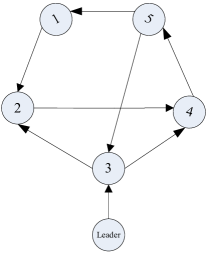
Figure 1: The structure of five-node digraph with leader node

For the structure in Fig.1, each node dynamic is considered as
Node 1:

$$\dot{x}_{11} =x_{12}-x_{11}^{2}x_{12}$$

$$\dot{x}_{12} =-(x_{11}+x_{12})(1-x_{11})^{2}+x_{12}^{2}u_{1},$$

Node 2:

$$\dot{x}_{21} =x_{22}-x_{21}^{2}x_{22}$$

$$\dot{x}_{22} =-(x_{21}+x_{22})(1-x_{21})^{2}+1.5x_{22}^{2}u_{2},$$

Node 3:

$$\dot{x}_{31} =x_{32}-x_{31}^{2}x_{32}$$

$$\dot{x}_{32} =-(x_{31}+x_{32})(1-x_{31})^{2}-0.2x_{32}^{2}u_{3},$$

Node 4:

$$\dot{x}_{41} =x_{42}-x_{41}^{2}x_{42}$$

$$\dot{x}_{42} =-(x_{41}+x_{42})(1-x_{41})^{2}+0.3x_{42}^{2}u_{4},$$

Node 5:

$$\dot{x}_{51} =x_{52}-x_{51}^{2}x_{52}$$

$$\dot{x}_{52} =-(x_{51}+x_{52})(1-x_{51})^{2}-0.9x_{52}^{2}u_{5},$$

While the state trajectory of the leader node is

$$\dot{x}_{01} =x_{02}-x_{01}^{2}x_{02}$$

$$\dot{x}_{02} =-(x_{01}+x_{02})(1-x_{01})^{2}.$$

Let $Q_{ii}=\left[\begin{array}[]{cc}1&0\\ 0&1\\ \end{array}\right]$, $i=1,\ldots,5$; $R_{ii}=8.5$, $i=1,\ldots,5$; $R_{ij}=0.1(i\neq j)$, $i,j=1,\ldots,5$ (Note that $R_{ij}=0$, if the ${v}_{j}$ is not the neighbor of ${v}_{i}$) and $a_{i}=0.1$, $i=1,\ldots,5$. Here, for the sake of simplicity, we let $\Phi=I_{n}$ and the generalized input variable be $e_{i}$.

Our intention is to design the optimal coordination control, making $x_{i}$ reach a consensus on leader and minimizing the cost functional (IV-A). By our method, we can obtain an optimal coordination control

$$u_{i}^{*}=-\frac{1}{2}R_{ii}^{-1}g_{i}^{T}(x_{i})(({l}_{ii}+b_{ii})\otimes I_{n}){\Lambda_{i}(e_{i})}{\theta}^{*}_{i},$$

$$i=1,\ldots,5.$$ (34)

We can see the evolution of weight $\hat{\theta}_{i}$ from Fig. 2. Obviously, after 10s, $\hat{\theta}_{i}$ converge to the ideal values.

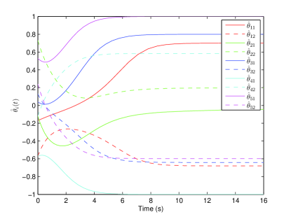
Figure 2: The convergence of GFHCE weight

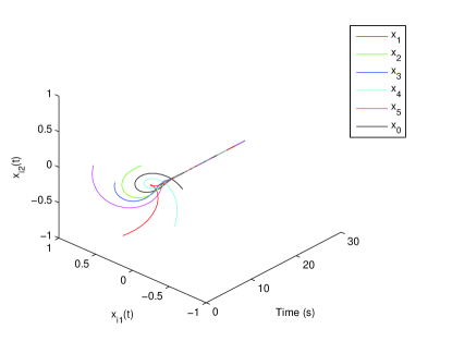
Figure 3: The evolution of the agent states

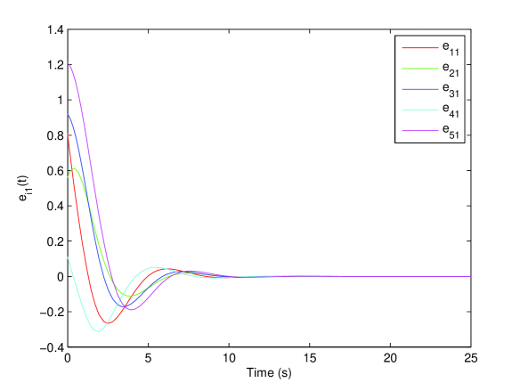
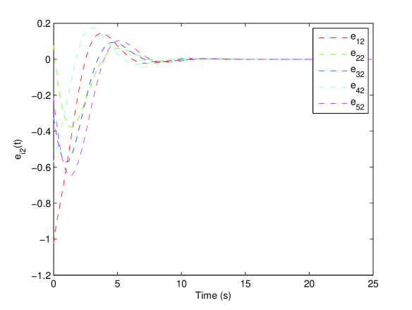
Figure 4: The evolution of the local consensus error: (a) error $e_{i1}$ and (b) error $e_{i2}$.

Fig. 3 depicts the evolution of the every agent’s state under the optimal coordination controls (VII) with the obtained ideal value ${\theta}_{i}$. After 15s, the state of each node reaches a consensus on leader node.

Fig. 4 shows the evolution of the local consensus error under the optimal coordination controls (VII) with the obtained ideal value ${\theta}_{i}$. After 15s, the consensus error $e_{i}$ goes to zero.

Remark 10

Obviously, only one GFHM is used as the approximator for each agent’s critic network (value function), whereas the action network presented in [23] and [39] is not required. It eliminates the action network architecture. Therefore, our scheme has greater advantage for multi-agent systems, comparing with dual network method in [23, 39] and [44].

VIII Conclusion

In this paper, the optimal coordination control has been presented for multi-agent systems by fuzzy adaptive dynamic programming. Our scheme is to approximate the solution of the coupled Hamilton-Jacobi equation, making use of the single GFHM as approximator, rather than using the dual-network model appeared in [23] and [39], under the framework of the PI algorithm. Then the approximation solution has been utilized to obtain the optimal coordination control. Since our method eliminates the action network model and reduces the number of weights updated, FADP based on the single GFHM has been a better scheme to design the optimal coordination control for multi-agent systems. An example has been presented to show the effectiveness of our scheme.

Appendix A

In order to prove the equation (IV-A) are equivalent to the equation

$$0= e_{i}^{T}Q_{ii}e_{i}+\frac{1}{4}V_{e_{i}}^{*T}((l_{ii}+b_{ii})\otimes I_{n})g_{i}(x_{i})R_{ii}^{-1}g_{i}^{T}(x_{i})((l_{ii}+b_{ii})\otimes I_{n})^{T}V^{*}_{e_{i}}$$

$$+\frac{1}{4}\sum\limits_{j\in N_{i}}V_{e_{j}}^{*T}((l_{jj}+b_{jj})\otimes I_{n})g_{j}(x_{j})R_{jj}^{-1}R_{ij}R_{jj}^{-1}g_{j}^{T}(x_{j})((l_{jj}+b_{jj})\otimes I_{n})^{T}V^{*}_{e_{j}}$$

$$+V_{e_{i}}^{*T}\mathcal{L}_{i}(f_{e}(t)+g(x)u^{*}),$$

we have to deduce $V_{e_{i}}^{*T}((l_{ii}+b_{ii})\otimes I_{n})(f_{ei}(t)+g_{i}(x_{i})u_{i}^{*})+V_{e_{i}}^{*T}\sum\limits_{j\in N_{i}}((l_{ij}+b_{ij})\otimes I_{n})(f_{ej}(t)+g_{j}(x_{j})u_{j}^{*})$ in (IV-A) from the term $V_{e_{i}}^{*T}\mathcal{L}_{i}(f_{e}(t)+g(x)u^{*})$. According to the previous definition of the paper, we know $f_{e}(t)=[f_{e1}^{T}(t),\cdots,f_{ei}^{T}(t),\cdots,f_{ej}^{T}(t),\cdots,f_{eN}^{T}(t)]^{T},$ $g(x)={\rm diag}\{g_{1}(x_{1}),\cdots,g_{i}(x_{i}),\cdots,g_{j}(x_{j}),\cdots,g_{N}(x_{N})\},$ $u^{*}=[u_{1}^{*T},\cdots,u_{i}^{*T},\cdots,u_{j}^{*T},\cdots,u_{N}^{*T}]^{T},L_{i}=[l_{i1},\ldots,l_{ii}\ldots,l_{ij}\ldots,l_{iN}]$ and $B$ is a diagonal matrix, while let $B_{i}=[b_{i1},\ldots,b_{ii}\ldots,b_{ij}\ldots,b_{iN}]$. Because $\mathcal{L}_{i}=(L_{i}+B_{i})\otimes I_{n}$, we can obtain $\mathcal{L}_{i}=[(l_{i1}+b_{i1})\otimes I_{n},\ldots,(l_{ii}+b_{ii})\otimes I_{n},\ldots,(l_{ij}+b_{ij})\otimes I_{n},\ldots,(l_{iN}+b_{iN})\otimes I_{n}]$. We also obtain

$$f_{e}(t)+g(x)u^{*}=\left[\begin{array}[]{c}f_{e1}(t)+g_{1}(x_{1})u_{1}^{*}\\ \vdots\\ f_{ei}(t)+g_{i}(x_{i})u_{i}^{*}\\ \vdots\\ f_{ej}(t)+g_{j}(x_{j})u_{j}^{*}\\ \vdots\\ f_{eN}(t)+g_{N}(x_{N})u_{N}^{*}\\ \end{array}\right].$$

Therefore,

$$V_{ei}^{*T}\mathcal{L}_{i}(f_{e}(t)+g(x)u^{*})$$

$$= V_{ei}^{*T}((l_{i1}+b_{i1})\otimes I_{n})(f_{e1}(t)+g_{1}(x_{1})u_{1}^{*})+\ldots+V_{ei}^{*T}((l_{ii}+b_{ii})\otimes I_{n})(f_{ei}(t)+g_{i}(x_{i})u_{i}^{*})$$

$$+\ldots+V_{ei}^{*T}((l_{ij}+b_{ij})\otimes I_{n})(f_{ej}(t)+g_{j}(x_{j})u_{j}^{*})+\ldots+V_{ei}^{*T}((l_{iN}+b_{iN})\otimes I_{n})(f_{eN}(t)+g_{N}(x_{N})u^{*}_{N})$$

$$= V_{ei}^{*T}\sum\limits_{j\in\mathcal{I}}((l_{ij}+b_{ij})\otimes I_{n})(f_{ej}(t)+g_{j}(x_{j})u_{j}^{*})$$

$$= V_{ei}^{*T}((l_{ii}+b_{ii})\otimes I_{n})(f_{ei}(t)+g_{i}(x_{i})u_{i}^{*})+V_{ei}^{*T}\sum\limits_{j\in\mathcal{I},i\neq j}((l_{ij}+b_{ij})\otimes I_{n})(f_{ej}(t)+g_{j}(x_{j})u_{j}^{*}).$$ (36)

Note that the expression includes all nodes in graph $\mathcal{G}_{x}$. When the node $v_{j}$ is not the neighbor of $v_{i}$, $l_{ij}=0(i\neq j)$. Because $B=[b_{ij}]$ is a diagonal matrix, $b_{ij}=0$, as $i\neq j$ (in order to understand easily, we retain $b_{ij}$ item). Therefore, removing the items which are not neighbors of $v_{i}$, the expression (A) can be rewritten as

$$V_{ei}^{*T}\mathcal{L}_{i}(f_{e}(t)+g(x)u^{*})=V_{e_{i}}^{*T}((l_{ii}+b_{ii})\otimes I_{n})(f_{ei}(t)+g_{i}(x_{i})u_{i}^{*})+V_{e_{i}}^{*T}\sum\limits_{j\in N_{i}}((l_{ij}+b_{ij})\otimes I_{n})(f_{ej}(t)+g_{j}(x_{j})u_{j}^{*}).$$

So, the expression (IV-A) holds.

References

• [1] Z. Lin, B. Francis and M. Maggiore, “Necessary and sufficient graphical conditions for formation control of unicycles,” IEEE Transactions on Automatic Control, vol. 50, no. 1, pp. 121–127, 2005.
• [2] D. Lee and M. Spong, “Stable flocking of multiple inertial agents on balanced graphs,” IEEE Transactions on Automatic Control, vol. 52, no. 8, pp. 1469–1475, 2007.
• [3] J. Zhu, J. Lu and X. Yu, “Flocking of multi-agent non-holonomic systems with proximity graphs,” IEEE Transactions on Circuits and Systems: Regular Papers, vol. 60, no. 1, pp. 199–210, 2013.
• [4] J. Lin, A. Morse and B. Anderson, “The multi-agent rendezvous problem$-$the asynchronous case,” 43rd IEEE Conference on Decision and Control (CDC), vol. 2, Atlantis, Paradise Island, Bahamas, 2004, pp. 1926–1931.
• [5] L. Xiao, S. Boyd, and S. Lall, “A scheme for robust distributed sensor fusion based on average consensus,” in Proceedings of the Fourth International Symposium on Information Processing in Sensor Networks, Los Angeles, CA, 2005, pp. 63–70.
• [6] Y. Cao, W. Yu, W. Ren and G. Chen, “An overview of recent progress in the study of distributed multi-agent coordination,” IEEE Transactions on Industrial Informatics, vol. 9, no. 1, pp. 427–438, 2013.
• [7] Z.  Meng, Z.  Li, A. Vasilakos and S. Chen, “Delay-induced synchronization of identical linear multiagent systems,” IEEE Transactions on Cybernetics, vol. 43, no. 2 pp.476–489, 2013.
• [8] G. Ferrari-Trecate, A. Buffa, and M. Gati, “Analysis of coordination in multi-Agent systems through partial difference equations,” IEEE Transactions on Automatic Control, vol 51, no, 6, pp.1058–1063, 2006.
• [9] Z.  Meng, Z.  Zhao and Z.  Lin, “On global leader-following consensus of identical linear dynamic systems subject to actuator saturation,” Systems and Control Letters, vol. 62, no. 2, pp.132–142, 2013.
• [10] N. A. Lynch, Distributed Algorithms, San Francisco, CA: Morgan Kaufmann, 1996.
• [11] M. DeGroot, “Reaching a consensus,” Journal of the American Statistical Association, vol.  69, no. 345, pp. 118–121, 1974.
• [12] V. Borkar and P. Varaiya, “Asymptotic agreement in distributed estimation,” IEEE Transactions on Automatic Control, vol. 27, no. 3, pp. 650–655, 1982.
• [13] J. Tsitsiklis, Problems in Decentralized Decision Making and Computation, Ph.D. dissertation, Dept. Electr. Eng. Comput. Sci., Lab. Inf. Decision Syst., Massachusetts Inst. Technol., Cambridge, MA, Nov. 1984.
• [14] R. Olfati-Saber and R. Murray, “Consensus problems in networks of agents with switching topology and time-delays,” IEEE Transactions on Automatic Control, vol. 49, no. 9, pp. 1520–1533, 2004.
• [15] W. Ren, R. Beard and E. Atkins, “A survey of consensus problems in multi-agent coordination,” in Proccedings of 2005 American Control Conference, vol. 3, Portland, OR, USA, 2005, pp. 1859–1864.
• [16] R. Olfati-Saber, J. Fax and R. Murray, “Consensus and cooperation in networked multi-agent systems,” in Proceedings of the IEEE. vol. 95, no. 1, 2007, pp. 215–233.
• [17] S. Tijs, Introduction to Game Theory, India: Hindustan Book Agency, 2003.
• [18] Q. Wei and D. Liu, “Nonlinear multi-person zero-sum differential games using iterative adaptive dynamic programming,” in Proceedings of the 30th Chinese Control Conference, Yantai, China, 2011, pp. 2456–2461.
• [19] K. Vamvoudakis and F. Lewis, “Multi-player non-zero-sum games: online adaptive learning solution of coupled Hamilton-Jacobi equations,” Automatica, vol. 47, no. 8, pp. 1556–1569, 2011.
• [20] K. Vamvoudakis, F. Lewis and G. Hudasc, “Multi-agent differential graphical games: Online adaptive learning solution for synchronization with optimality,” Automatica, vol. 48, no. 8, pp. 1598–1611, 2012.
• [21] E. Semsar-Kazerooni and K. Khorasani, “Multi-agent team cooperation: A game theory approach,” Automatica, vol. 45, no.10, pp. 2205–2213, 2009.
• [22] S. Parsons and M. Wooldridge, “Game theory and decision theory in multi-agent systems,” Autonomous Agents and Multi-Agent Systems, vol. 5, no. 3, pp. 243–254, 2002.
• [23] H. Zhang, L. Cui, X. Zhang and Y. Luo, “Data-driven robust approximate optimal tracking control for unknown general nonlinear systems using adaptive dynamic programming method,” IEEE Transactions on Neural Networks, vol. 22, no. 12, pp. 2226–2236, 2011.
• [24] D. Wang, D. Liu and Q. Wei, “Finite-horizon neuro-optimal tracking control for a class of discrete-time nonlinear systems using adaptive dynamic programming approach,” Neurocomputing, vol. 78, no. 1, pp. 14–22, 2012.
• [25] D. Kirk, Optimal Control Theory-An Introduction, New York: Dover, 2004.
• [26] J. Si, A. Barto, W. Powell, and D. Wunsch, Handbook of Learning and Approximate Dynamic Programming, New York: Wiley, 2004.
• [27] F. Lewis and D. Vrabie, “Reinforcement learning and adaptive dynamic programming for feedback control,” IEEE Circuits Systems Magazine, vol. 9, no. 3, pp. 32–50, 2009.
• [28] F. Wang, H. Zhang, and D. Liu, “Adaptive dynamic programming: an introduction,” IEEE Computational Intelligence Magazine, vol. 4, no. 2, pp. 39–47, 2009.
• [29] W. Rudin, Principles of Mathematical Analysis, New York: McGraw-Hill, Inc., 1976.
• [30] H. Zhang and D. Liu, Fuzzy Modeling and Fuzzy Control, Boston: Birkhäuser, 2006.
• [31] H. Zhang and Y. Quan, “Modeling identification and control of a class of nonlinear system,” IEEE Transaction on Fuzzy Systems, vol. 9, no. 2 pp. 349–354, 2001.
• [32] H. Zhang, Z. Wang, M. Li, Y. Quan and M. Zhang, “Generalized fuzzy hyperbolic model: A universal approximator,” ACTA Automatica Sinica, vol. 30, no. 3, pp. 416–422, 2004 (in Chinese).
• [33] J. Zhang, H. Zhang, Y. Luo and H. Liang, “Optimal control design for nonlinear systems: Adaptive dynamic programming based on fuzzy critic estimator,” The 2012 International Joint Conference on Neural Networks (IJCNN), Brisbane, 2012, pp. 1–6.
• [34] J. Zhang, H. Zhang, Y. Luo and H. Liang, “Nearly optimal control scheme using adaptive dynamic programming based on generalized fuzzy hyperbolic model,” ACTA Automatica Sinica, vol. 39, no 2, pp. 142–149, 2013.
• [35] M. Margaliot and G. Langholz, “A new approach to fuzzy modeling and control of discrete-time systems,” IEEE Transactions on Fuzzy Systems, vol. 11, no. 4, pp. 486–494, 2003.
• [36] H. Zhang, F. Lewis and Z. Qu, “Lyapunov, adaptive, and optimal design techniques for cooperative systems on directed communication graphs,” IEEE Transactions on Industrial Electronics, vol. 59, no. 7, pp. 3026–3041, 2012.
• [37] G. Ferrari-Trecate, L. Galbusera, M. Marciandi, and R. Scattolini, “Model predictive control schemes for consensus in multi-agent systems with single- and double-integrator dynamics,” IEEE Transactions on Automatic Control, vol. 54, no. 11, pp. 2560–2572, 2009
• [38] D. Bertsekas and J. Tsitsiklis, Neuro-dynamic Programming, MA: Athena Scientific, 1996.
• [39] K. Vamvoudakis and F. Lewis, “Online actor-critic algorithm to solve the continuous-time infinite horizon optimal control problem,” Automatica, vol. 46, no. 5, pp. 878–888, 2010.
• [40] A. Das and F. Lewis, “Distributed adaptive control for synchronization of unknown nonlinear networked systems,” Automatica, vol. 46, no. 12, pp. 2014–2021, 2010.
• [41] F. Abdollahi, H. Talebi and R. Patel, “A stable neural network observer with application to flexible-joint manipulators,” in Proceedings of the 9th International Conference on Neural Information Processing, vol. 4, 2002, pp. 1910–1914.
• [42] H. K. Khalil, Nonlinear Systems (Third Edition), New Jersey: Prentice Hall, 2002.
• [43] F. Lewis, S. Jagannathan and A. Yesildirek, Neural Network Control of Robot Manipulators and Nonlinear Systems, Bristol, PA, USA: Taylor and Francis, Inc, 1999.
• [44] T. Dierks and S. Jagannathan, “Optimal tracking control of affine nonlinear discrete-time systems with unknown internal dynamics,” Joint 48th IEEE Conference on Decision and Control and 28th Chinese Control Conference, Shanghai, China, 2009, pp. 6750–6755.
• [45] P. Ioannou and B. Fidan, Adaptive Control Tutorial, Philadelphia: SIAM, 2006.
• [46] C. Cox and R. Saeks, “Adaptive critic control and functional link neural networks,” IEEE International Conference on Systems, Man, and Cybernetics, vol. 2, 1998, pp. 1652–1657.