Lattice Model for Production of Gas

Abstract

We define a lattice model for rock, absorbers, and gas that makes it possible to examine the flow of gas to a complicated absorbing boundary over long periods of time. The motivation is to deduce the geometry of the boundary from the time history of gas absorption. We find a solution to this model using Green’s function techniques, and apply the solution to three absorbing networks of increasing complexity.

Introduction.

Hydrofracturing Turcotte et al. (2014); Marder et al. (2016) liberates gas from mudstones, often called shales, that are brittle residues of seabeds buried thousands of meters deep and around 30 meters thick. The extraction process involves creating a fracture network that extends over a distance on the order of a kilometer in one direction, and on the order of 200 meters in the perpendicular direction. Diffusion in the mudstone is very slow, but once gas reaches the fractures it travels rapidly to a wellbore and from there up to the surface. The time history of gas production can be used to extract information about the dimensions and structure of the fractured network Patzek et al. (2013, 2014).

This setting motivates the creation of a simple model for the flow of gas from an infinite two-dimensional plane into a bounded but geometrically complex absorbing boundary. The problem bears a family resemblance to Diffusion-Limited Aggregation Witten Jr and Sander (1981); Sahimi (1993); Halsey2000 because it involves diffusion on a lattice into a cluster. However in this problem the cluster is specified at the outset and does not change. Because the dynamics are linear, the model is analytically tractable using Green’s functions Economou (1983); Berciu and Cook (2010); Joyce (2017). The task is to find the time dependence for the gas reaching the absorbers because this models the process of gas production.

Figure 1: Production rate of a single absorber over very long time.

Model Definition.

We pose the model on a two-dimensional square lattice, whose nodes are indexed by $j.$ On every node we place a time-dependent density of gas $\rho_{j}(t).$ We denote the state vector of densities by $|\rho(t)\rangle,$ and the density at location $j$ by $\rho_{j}(t)=\langle j|\rho(t)\rangle$. The problem begins at time $t=0$ with a uniform initial density $|\rho_{\rm i}\rangle\equiv|\rho(0)\rangle;\quad\langle j|\rho_{\rm i}\rangle=\rho_{j}(0)=1.$ Every site is either rock through which gas diffuses or else an absorber that collects all gas reaching it and sends none back. To keep track of absorbers we define $\theta_{j}$ by

$$\theta_{j}=\begin{cases}1&\text{if $j$ is unbroken rock)}\\ 0&\text{if $j$ is an absorber) }\end{cases}.$$ (1)

Between every pair of nodes $j,j^{\prime}$ there is a link of strength $k_{jj^{\prime}}=k_{j^{\prime}j}$. We restrict ourselves here to nearest-neighbor coupling so $k_{jj^{\prime}}$ is 1 if $j$ and $j^{\prime}$ are nearest neighbors and 0 otherwise. The time evolution of $\rho$ is given by

$$\frac{\partial}{\partial t}|\rho\left(t\right)\rangle=\hat{H}|\rho\left(t\right)\rangle,$$ (2)

where

$$\langle j|\hat{H}|j^{\prime}\rangle=\theta_{j}\left[k_{jj^{\prime}}-B\delta_{jj^{\prime}}\right]\theta_{j^{\prime}};\quad B\equiv\sum_{j^{\prime}}k_{jj^{\prime}}=4.$$ (3)

The $\theta$ functions ensure that when gas reaches an absorber it disappears. Note that $\hat{H}$ is real and symmetric, with all off-diagonal entries either 0 or 1. The Hamiltonian $\hat{H}$ has as many zero eigenvalues as there are absorbers. If however one projects down onto the space of all sites $j$ where $\theta_{j}=1,$ then these zero eigenvalues disappear. In this space $\hat{H}$ has a complete set of eigenvectors $|\alpha\rangle$ with eigenvalues $E_{\alpha}$. This observation is not computationally useful when the spectrum is continuous. However if one has a closed region completely surrounded by absorbers, with a finite number $N_{s}$ of interior lattice points, then the spectrum is discrete, eigenvalues and eigenvectors can be computed explicitly, and the rate at which gas is produced is

$$\dot{\phi}_{{\rm interior}}=-\sum_{\alpha=1}^{N_{s}}E_{\alpha}e^{E_{\alpha}t}|\langle\alpha|\rho_{\rm i}\rangle|^{2}.$$ (4)

Green’s function solution for continuous spectrum.

(a) Network exhibiting the schematic geometry for hydrofractured horizontal well from Patzek et al. (2013).

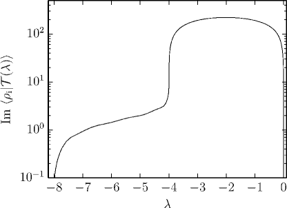
(b) Spectral function from Eq. (7) for network of Figure (2a).

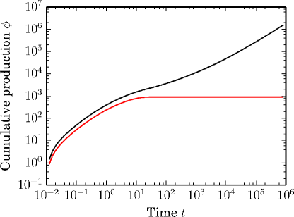
(c) Cumulative gas production for network of Figure (2a) (color online). The lower (red) curve gives the production from the interior only.

Figure 2: Gas production from assembly of absorbers that mimics a simplified geometry for hydrofractured wells.

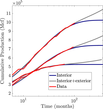
Figure 3: Three wells from the Barnett shale that have produced long enough that the contribution from the exterior region is starting to become visible. Mcf=1000 cubic feet. (Color online).

The exterior region of the absorbing network has an infinite number of sites, the spectrum has a continuous component, and explicit calculation of all eigenvalues is impossible. Obtaining the continuous spectrum requires a different approach. Define the Green function Economou (1983) $\hat{G}(E)=\left(E-\hat{H}\right)^{-1}$and the unperturbed Green function $\hat{G}_{0}(E)=\left(E-\hat{H}_{0}\right)^{-1}$ for the lattice without any absorbers. The full Hamiltonian is $\hat{H}=\hat{H}_{0}+\hat{H}_{1}$ where

$$\hat{H}_{1}=-\sum_{jj^{\prime}}|j\rangle\left(k_{jj^{\prime}}-B\delta_{jj^{\prime}}\right)\left(1-\theta_{j}\theta_{j^{\prime}}\right)\langle j^{\prime}|.$$ (5)

Note that $\hat{H}_{1}$ is nonzero only in the space spanned by absorbers and their nearest neighbors. One can obtain the continous spectrum from computations in this finite-dimensional space. The full Green function can be obtained from the scattering $\hat{T}$ matrix defined by $\hat{G}=\hat{G}_{0}+\hat{G}_{0}\hat{T}\hat{G}_{0}.$ To find gas production it turns out one does not need the complete $\hat{T}$ matrix, but just the state vector produced by its action on the initial state $|{\cal T}(E)\rangle\equiv\hat{T}(E)|\rho_{{\rm i}}\rangle.$ This state vector is determined by the linear system

$$\left(1-\hat{H}_{1}\hat{G}_{0}(E)\right)|{\cal T}(E)\rangle=\hat{H}_{1}|\rho_{\rm i}\rangle$$ (6)

and then gas production due to the continous spectrum of the exterior is provided by

$$\dot{\phi}_{{\rm exterior}} =-\int_{-8}^{0}\frac{d\lambda}{\pi\lambda}e^{\lambda t}\,\textrm{Im}\lim_{\eta\rightarrow 0}\langle\rho_{{\rm i}}|{\cal T}(\lambda-i\eta)\rangle.$$ (7)

Because of the limit $\eta\rightarrow 0,$ which also applies implicitly to subsequent equations, Eq. (7) includes no contributions from the gas at interior sites captured by Eq. (4). The spectrum of the interior sites is discrete, consists of a finite sum of delta functions, and these vanish in the limiting process. The exterior problem can also have a discrete spectrumSutherland (1986), missing from this expression, as we discuss later.

Computation of Eq. (6) requires computing matrix elements $\lim_{\eta\rightarrow 0}\langle j|\hat{G}_{0}(\lambda-i\eta)|j^{\prime}\rangle$ of the unperturbed lattice Green function. This can be done using recursion relations due to Morita Morita (1975), and described in compact form by Berciu Berciu and Cook (2010). These recursion relations are exponentially unstable, and the instability is particularly severe as $\lambda$ approaches the band edge at $\lambda=0$. One must get very close to the band edge since values as small as $\lambda\approx-10^{-1000}$ are needed for the integral in Eq. (7) to converge. The solution we have adopted is to employ Morita’s recursions with high-precision arithmetic. For absorber networks extending across 100 lattice sites, the recursions require from 100 to 5000 places of precision. Once the Green function matrix elements have been obtained, the rest of the computation can be carried out in ordinary double precision.

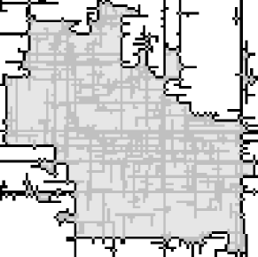
(a) Network of absorbers created by 550 horizontal and vertical cracks.

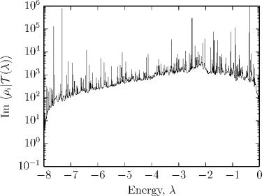
(b) Continuous spectrum for network in part (a). The sharp peaks come from small features on the exterior of the network shielded by extended arms.

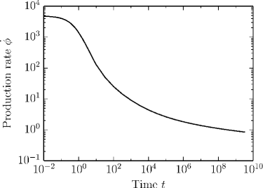
(c) Total gas production from network in part (a).

Figure 4: Gas absorption into network of criss-crossing fractures.

One absorber.

As a first application of the formalism, consider the case of a single absorber in an infinite square lattice. The vector $\langle j|{\cal T\rangle}$ has five components. The first corresponds to the absorber at 0, and the remaining four correspond to the four neighbors of the absorber. Only $\langle 0|{\cal T}\rangle$ has nonzero imaginary part; the remaining values $\langle j|{\cal T}\rangle=-1,$ where $j=1\dots 4,$ and

$$\langle 0|{\cal T}(\lambda)\rangle=\lambda+4-\frac{1}{\langle 0|\hat{G_{0}}(\lambda)|0\rangle}.$$ (8)

This leads to total gas production $\dot{\phi}=\dot{\phi}_{{\rm exterior}}$

$$\dot{\phi}=\int_{-\ln 8}^{\infty}\frac{df}{\pi}e^{-te^{-f}}\text{Im}\frac{-1}{\langle 0|\hat{G}_{0}(-e^{-f})|0\rangle}$$ (9)

which for large values of $t$ equals approximately

$$\dot{\phi} \approx\int_{-\ln 8}^{\infty}\frac{df}{\pi}\,e^{-te^{-f}}\frac{1}{\tau_{0}+\tau_{1}f+\tau_{2}f^{2}};$$ (10)

where $$\tau_{0}=\frac{\left(\ln 32\right)^{2}}{4\pi^{2}}+\frac{1}{4},\ \tau_{1}=\frac{\ln 32}{2\pi^{2}},\ \tau_{2}=\frac{1}{4\pi^{2}}.$$

A plot of Eq. (9) appears in Figure (1).

Absorbing network with ten stages.

As a second example, consider the network pictured in Figure (2a). It is 100 units wide, 10 units high, and has 10 internal regions of equal size. The interior problem is of size $810\times 810.$ By counting up the number of absorbing faces exposed to gas, one finds that initial production from the interior must be $\dot{\phi}_{{\rm interior}}(0)=360.$

The exterior problem leads to a linear system of equations of size $323\times 323.$ Again counting the number of absorbing faces exposed to gas on the outside shows that initial production from the exterior is $\dot{\phi}_{{\rm exterior}}(0)=224$. The same integer comes from Eq. (7) when $t=0;$ this sum rule provides a good check on the accuracy of the computations and shows that the exterior problem has no discrete spectrum in this case. The spectral function $\langle\rho_{{\rm i}}|{\cal{T}}(\lambda)\rangle$ appears in Figure (2b). The interior and total production appear in Figure (2c). The well geometry of Figure (2a) is precisely the type of geometry used in Ref Patzek et al. (2013) to fit production of thousands of wells. However, only production from the interior of the well was previously considered. Here we see that on sufficiently long time scales, gas arriving from the exterior region leads to a characteristic upturn on a log-log plot. Analysis of well production data to extract this characteristic long-time signature is underway. From the analysis it appears that if one considers a gas-producing well over the course of thirty years, the extra gas produced by exterior flow will contribute extra production on the order of 20%. Figure (3) displays production data from three wells for which the long-time behavior including production from the exterior region is just starting to become visible at the ten year mark; these are some of the oldest existing wells.

Complex fracture network.

The essential behavior of the examples presented so far could be examined without much difficulty from a continuum perspective Carslaw and Jaeger (1959) or using finite element programs such as COMSOL. For a final example, depicted in Figure (4a) we present a geometrically complex structure produced by 550 intersecting horizontal and vertical cracks with a power-law length distribution motivated by geophysical data Eftekhari (2016). The probability that a fracture have length $l$ is proportional to $l^{-2.2}$. The interior portion, shown with grayscale in the figure has 3080 sites in light gray that are rock, interspersed by interior absorbers in darker gray. Absorbers forming the exterior of the network are colored in black. The 3080 eigenvalues and eigenvectors of the interior problem needed for Eq. (4) can be computed in seconds on a single processor. The sum rule $\dot{\phi}_{{\rm interior}}(0)=3264$ provides a check on the accuracy of these computations. The integrand of Eq. (7) has hundreds of narrow spikes that make its computation more difficult although still tractable. Counting up the number of exterior faces on the absorbers gives the sum rule $\dot{\phi}_{{\rm exterior}}(0)=1556$, but the integral of the continuous spectrum gives only 1546.53. This is because the external problem has localized eigenfunctions precisely at $\lambda=-4$. Their weight can be determined by taking $\eta=10^{-8}$ in Eq. (7) and performing the integral in a small neighborhood of $\lambda=-4.$ The contribution from the exterior localized eigenfunctions is 9.47, and adding this to the integral of the continuous spectrum finally exhausts the sum rule.

For large $f=\ln\left(-\lambda\right)$, the continuous spectrum assumes the asymptotic form of Eq. (10) with $\tau_{2}=.02533,\quad\tau_{1}=-0.3947,\quad\tau_{0}=1.7877.$ This form is all one needs for the very long time behavior. The continuous spectrum appears in Figure (4b) and the production rate as a function of time, summing contributions from the discrete and continuous spectra, appears in Figure (4c).

We anticipate that the ability to find precise solutions for the production history of complex networks of absorbers will assist in studying the relationship between production data and the complex geometries of real fractured networks.