Quantum Limitation to the Coherent Emission of Accelerated Charges

Abstract

Accelerated charges emit electromagnetic radiation. According to classical electrodynamics if the charges move along sufficiently close trajectories they emit coherently, i.e., their emitted energy scales quadratically with their number rather than linearly. By investigating the emission by a two-electron wave packet in the presence of an electromagnetic plane wave within strong-field QED, we show that quantum effects deteriorate the coherence predicted by classical electrodynamics even if the typical quantum nonlinearity parameter of the system is much smaller than unity. We explain this result by observing that coherence effects are also controlled by a new quantum parameter which relates the recoil undergone by the electron with the width of its wave packet in momentum space.

Optical laser pulses with intensities of the order of $10^{22}\,\text{W/cm}^{2}$ have been already achieved Yanovsky et al. (2008) and intensities of the order of $10^{24}\,\text{W/cm}^{2}$ are envisaged Extreme Light Infrastructure , http://www.eli-laser.eu/(2017) (ELI); Exawatt Center for Extreme Light Studies , http://www.xcels.iapras.ru/(2017) (XCELS). At such high intensities the interaction between the laser field and an electron (mass $m$ and charge $e<0$) is highly-nonlinear and electrodynamical processes involving electrons/positrons occur with the exchange of several photons between the laser field and electrons/positrons themselves Ritus (1985); Di Piazza et al. (2012). This has also primed a surge of interest in testing QED in the so-called “strong-field” regime where the background field intensity is effectively of the order of $\mathcal{I}_{cr}=4.6\times 10^{29}\,\text{W/cm}^{2}$, corresponding to the electric field $\mathcal{E}_{cr}=m^{2}c^{3}/\hbar|e|=1.3\times 10^{16}\,\text{V/cm}$ Di Piazza et al. (2012). Due to the Lorentz invariance of the theory, in fact, strong-field QED can be effectively probed at laser intensities $\mathcal{I}\ll\mathcal{I}_{cr}$ by employing ultrarelativistic electron beams with correspondingly high energies $\varepsilon\sim mc^{2}\sqrt{\mathcal{I}_{cr}/\mathcal{I}}\gg mc^{2}$ Di Piazza et al. (2012). Indeed, electron beams with energies beyond $1\,\text{GeV}$ have been already produced both via conventional Patrignani et al. (2017) and laser-based accelerators Leemans et al. (2014). One of the fundamental processes which can be exploited to test strong-field QED is Nonlinear Single Compton Scattering (NSCS), where an electron traveling inside a laser field exchanges multiple photons with the laser field itself while also emitting a single, non-laser photon. NSCS has been studied in the presence of a monochromatic plane wave Goldman (1964); Brown and Kibble (1964); Nikishov and Ritus (1964); Fried and Eberly (1964); Ritus (1985); Ivanov et al. (2004); Harvey et al. (2009); Corson et al. (2011); Wistisen (2014), of a pulsed plane wave Boca and Florescu (2009); Heinzl et al. (2010); Boca and Florescu (2011); Mackenroth and Di Piazza (2011); Seipt and Kämpfer (2011); Boca and Florescu (2011); Dinu et al. (2012); Boca et al. (2012); Dinu (2013); Krajewska et al. (2014); Titov et al. (2014); Angioi et al. (2016), and of a space-time-focused laser beam Di Piazza (2017) (see also Di Piazza (2014, 2015); Heinzl and Ilderton (2017a, b)). In Brown and Kibble (1964); Nikishov and Ritus (1964); Fried and Eberly (1964); Ritus (1985); Ivanov et al. (2004); Harvey et al. (2009); Wistisen (2014); Boca and Florescu (2009); Heinzl et al. (2010); Boca and Florescu (2011); Mackenroth and Di Piazza (2011); Seipt and Kämpfer (2011); Boca and Florescu (2011); Dinu et al. (2012); Boca et al. (2012); Dinu (2013); Krajewska et al. (2014); Titov et al. (2014) an incoming electron in a plane wave with a definite momentum was investigated, whereas in Corson et al. (2011); Angioi et al. (2016) NSCS by a localized electron wave packet was studied. In all these works, the radiation emitted by a single electron has been considered, such that coherence effects in the nonlinear emission by several electrons have never been investigated within strong-field QED.

In this Letter we explore the novel features in the quantum radiation spectrum brought about by considering two-electron wave packets properly anti-symmetrized as an initial state. For a single electron with definite asymptotic four-momentum $p^{\mu}$ the quantum spectra tend to the classical ones if $\chi=(kp)\mathcal{E}/m\omega\mathcal{E}_{cr}\ll 1$ Ritus (1985); Di Piazza et al. (2012). Here, $\mathcal{E}$ and $k^{\mu}=(\omega,\bm{k})$ are the laser field’s amplitude and its central four-wave-vector, respectively (units with $\hbar=c=1$ and $\alpha=e^{2}\approx 1/137$ are employed throughout and the metric tensor reads $\eta^{\mu\nu}=\text{diag}(+1,-1,-1,-1)$). Now, according to classical physics, if $N$ charges move inside a field along sufficiently close trajectories, the radiated energy can scale as $N^{2}$ (rather than $N$) up to arbitrarily high frequencies Klepikov (1985). Below, we consider the paradigmatic case where the two electrons are characterized by the same initial distribution of momenta and thus by the same average quantum parameter $\chi^{\prime}$. We show that at very different size scales of the electrons’ wave packet quantum effects limit or completely suppress the coherence of the emission even for $\chi^{\prime}\ll 1$, i.e., when single-particle classical and quantum spectra approximately coincide. We note that in general for an initial multi-particle state the condition $\chi^{\prime}\ll 1$ is not sufficient to recover the classical limit. However, our results explicitly indicate that the intuitive implication that when every particle emits classically then the whole system does too is invalid. We explain this unexpected result by observing that the condition $\chi^{\prime}\ll 1$ ensures that the typical emitted photon energies are much smaller than the common average energy of electron wave packets. However, coherence effects are also controlled by a new quantum parameter which relates the recoil undergone by the electron not with the average energy but with the width of its wave packet in momentum space. These coherence effects, which become even larger at $\chi^{\prime}\sim 1$, allow for high-precision tests of the strong-field sector of QED at the level of quantum amplitudes, which employ few-electron pulses in a well-controlled quantum state.

The laser field is assumed to be linearly polarized along the $x$ direction and to propagate along the $z$ direction. Within the plane-wave approximation, it can be described by the classical four-potential $\mathcal{A}^{\mu}_{L}(\phi)=(0,\bm{\mathcal{A}}^{\mu}_{L}(\phi))=\mathcal{A}^{\mu}\psi_{L}(\phi)$, where $\mathcal{A}^{\mu}=(0,-\mathcal{E}/\omega,0,0)$, $\psi_{L}(\phi)$ is a smooth function with compact support and $\phi=(nx)$, with $n^{\mu}=k^{\mu}/\omega=(1,0,0,1)$. For the sake of definiteness, we set $\phi=0$ as the initial light-cone “time” and thus assume that $\psi_{L}(\phi)=0$ for $\phi\leq 0$. The initial two-electron state is characterized by two definite spin quantum numbers $s_{j}$ ($j\in\{1,2\}$) and has the form

$$|\Psi\rangle=\frac{1}{\sqrt{\mathcal{N}}}\prod_{j=1}^{2}\bigg{[}\int\frac{d^{3}p_{j}}{(2\pi)^{3}\sqrt{2\varepsilon_{j}}}\rho_{j}(\bm{p}_{j})a_{s_{j}}^{\dagger}(\bm{p}_{j})\bigg{]}|0\rangle.$$ (1)

Here, $\mathcal{N}$ is a normalization factor such that $\langle\Psi|\Psi\rangle=1$, the operator $a^{\dagger}_{s_{j}}(\bm{p}_{j})$ creates an electron with momentum $\bm{p}_{j}$ (energy $\varepsilon_{j}=\sqrt{m^{2}+\bm{p}_{j}^{2}}$) and spin quantum number $s_{j}$, $\rho_{j}(\bm{p}_{j})$ is an arbitrary square-integrable complex-valued function describing each initial electron momentum distribution, and $|0\rangle$ is the free vacuum state. From the anti-commutation relations $\{a_{s}(\bm{p}),a^{\dagger}_{s^{\prime}}(\bm{p}^{\prime})\}=(2\pi)^{3}\delta^{(3)}(\bm{p}-\bm{p}^{\prime})\,\delta_{ss^{\prime}}$ Peskin and Schroeder (1995), the normalization factor $\mathcal{N}$ turns out to have the form $\mathcal{N}=\mathcal{N}_{12}-\delta_{s_{1}s_{2}}\mathcal{N}_{21}$, with

$$\mathcal{N}_{ij}=\int\frac{d^{3}p_{1}}{(2\pi)^{3}2\varepsilon_{1}}\frac{d^{3}p_{2}}{(2\pi)^{3}2\varepsilon_{2}}\rho_{1}^{*}(\bm{p}_{1})\rho_{i}(\bm{p}_{1})\rho_{2}^{*}(\bm{p}_{2})\rho_{j}(\bm{p}_{2}).$$ (2)

If $c_{l^{\prime}}^{\dagger}(\bm{k}^{\prime})$ is the operator which creates a photon with momentum $\bm{k}^{\prime}$ (energy $\omega^{\prime}=\sqrt{\bm{k}^{\prime 2}})$ and polarization $l^{\prime}$, the final state in NSCS has the form

$$|\Psi^{\prime}\rangle=\sqrt{8\omega^{\prime}\varepsilon^{\prime}_{1}\varepsilon^{\prime}_{2}}\,c_{l^{\prime}}^{\dagger}(\bm{k}^{\prime})a_{s^{\prime}_{2}}^{\dagger}(\bm{p}^{\prime}_{2})a_{s^{\prime}_{1}}^{\dagger}(\bm{p}^{\prime}_{1})|0\rangle,$$ (3)

with $\varepsilon^{\prime}_{j}=\sqrt{m^{2}+\bm{p}_{j}^{\prime\,2}}$. The leading-order $S$-matrix element $S$ of NSCS within the Furry picture Furry (1951); Berestetskii et al. (1982) reads

$$S=-ie\int d^{4}x\langle\Psi^{\prime}|\bar{\Psi}(x)\gamma^{\mu}\Psi(x)A_{\mu}(x)|\Psi\rangle,$$ (4)

where the Dirac field $\Psi(x)$ is expanded with respect to Volkov states (see Furry (1951); Berestetskii et al. (1982); Ritus (1985) and the Supplemental Material (SM) ), where $\bar{\Psi}(x)=\Psi^{\dagger}(x)\gamma^{0}$, where $\gamma^{\mu}$ are the Dirac matrices, and where $A^{\mu}(x)$ is the quantized part of the electromagnetic field. Here, we neglect the interaction between the electrons as their dynamics is predominantly determined by the intense plane wave.

At the leading order of perturbation theory, only one of the two electrons emits a photon (see Fig. 1), the state of the other electron remaining unchanged.

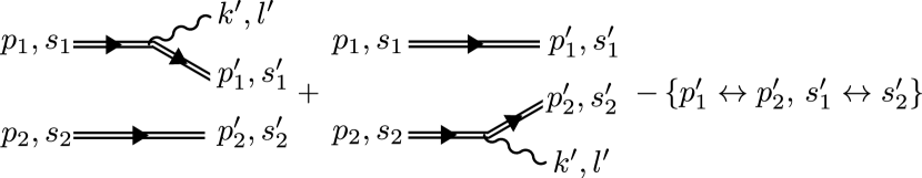
Figure 1: Leading-order Feynman diagrams of NSCS by two electrons. The double lines indicate Volkov states and the symbol $\{p^{\prime}_{1}\leftrightarrow p^{\prime}_{2},s^{\prime}_{1}\leftrightarrow s^{\prime}_{2}\}$ indicates the exchange diagrams.

Also, since the plane wave depends on the spacetime coordinates only via $\phi=t-z$, the amplitudes involving the photon emission include a three-dimensional Dirac delta-function, which enforces the conservation of the transverse ($\perp$) components ($x$- and $y$-components) and of the minus ($-$) component (time- minus $z$-component) of the four-momenta of the involved particles (see also the SM). Thus, by introducing the two on-shell four-momenta $q_{j}^{\mu}$ ($q_{j}^{2}=m^{2}$) such that $\bm{q}_{j,\perp}=\bm{p}^{\prime}_{j,\perp}+\bm{k}^{\prime}_{\perp}$ and $q_{j,-}=p^{\prime}_{j,-}+k^{\prime}_{-}$, i.e.,

$$q^{\mu}_{j}=p^{\prime\,\mu}_{j}+k^{\prime\,\mu}-\frac{(k^{\prime}p^{\prime}_{j})}{p^{\prime}_{j,-}+k^{\prime}_{-}}n^{\mu},$$ (5)

the amplitude $S$ can be written in the form $S=S_{12}-S_{21}$, where

$$S_{12}=\frac{e}{i}\sqrt{\frac{4\pi}{\mathcal{N}}}\sum_{j=1}^{2}\rho_{j}(\bm{q}_{j})\rho_{j^{\prime}}(\bm{p}^{\prime}_{j^{\prime}})\delta_{s^{\prime}_{j^{\prime}}s_{j^{\prime}}}\frac{M_{s^{\prime}_{j}l^{\prime},s_{j}}(p^{\prime}_{j},k^{\prime};q_{j})}{2q_{j,-}},$$ (6)

with $j^{\prime}=3-j$, and where $S_{21}=S_{12}(p^{\prime}_{1}\leftrightarrow p^{\prime}_{2},q_{1}\leftrightarrow q_{2},s^{\prime}_{1}\leftrightarrow s^{\prime}_{2})$. Here, we have introduced the reduced amplitude $M_{s^{\prime}l^{\prime},s}(p^{\prime},k^{\prime};p)$ characteristic of NSCS by a single electron with definite initial (final) four-momentum $p^{\mu}$ ($p^{\prime\,\mu}$) and spin quantum number $s$ ($s^{\prime}$), which emits a photon with four-momentum $k^{\prime}$ and polarization $l^{\prime}$ (see, e.g., Mackenroth and Di Piazza (2011) and the SM).

The emitted photon energy spectrum $dE_{Q}/d\omega^{\prime}$ of interest here reads

$$\frac{dE_{Q}}{d\omega^{\prime}}=\frac{\omega^{\prime\,2}}{8}\sum_{\{s_{j}s^{\prime}_{j}l^{\prime}\}}\int\frac{d\Omega^{\prime}}{(2\pi)^{3}2}\frac{d^{3}p^{\prime}_{1}}{(2\pi)^{3}2\varepsilon^{\prime}_{1}}\frac{d^{3}p^{\prime}_{2}}{(2\pi)^{3}2\varepsilon^{\prime}_{2}}\lvert S\rvert^{2},$$ (7)

where $\Omega^{\prime}$ denotes the solid angle corresponding to $\bm{n}^{\prime}=\bm{k^{\prime}}/\omega^{\prime}$. Note that if the electrons were distinguishable, the energy emission spectrum would have the same form as in Eq. (7), with the replacement $|S|^{2}\to 2(\mathcal{N}/\mathcal{N}_{12})|S_{12}|^{2}$.

In order to investigate the coherence properties of the emitted radiation, we consider the paradigmatic case in which the two electron wave packets in position space differ only by a translation by a vector $\bm{r}^{\prime}$, i.e., $\rho_{2}(\bm{p}_{2})=\rho_{1}(\bm{p}_{2})\exp(-i\bm{p}_{2}\cdot\bm{r}^{\prime})$, such that $|\rho_{1}(\bm{p})|^{2}=|\rho_{2}(\bm{p})|^{2}$. Also, without loss of generality we choose the function $\rho_{1}(\bm{p}_{1})$ to be real and we denote it as $\rho(\bm{p}_{1})$.

Let us first study the classical energy spectrum $dE_{C}/d\omega^{\prime}$ emitted by two electrons in a plane wave with initial (at $t=0$) positions $\bm{r}^{\prime}_{1}=\bm{0}$ and $\bm{r}^{\prime}_{2}=\bm{r}^{\prime}$, with $z^{\prime}>0$, and four-momenta $p_{j}^{\prime\,\mu}=(\varepsilon^{\prime}_{j},\bm{p}^{\prime}_{j})$. Classical coherence effects in the emitted frequency $\omega^{\prime}$ are controlled by the two phases $\omega^{\prime}\Phi_{j}(\phi)$, with (see the SM)

$$\Phi_{j}(\phi)=\int_{0}^{\phi}d\phi^{\prime}\frac{(n^{\prime}p^{\prime}_{j}(\phi^{\prime}))}{p^{\prime}_{j,-}}+\bigg{[}\frac{(n^{\prime}p^{\prime}_{j})}{p^{\prime}_{j,-}}\bm{n}-\bm{n}^{\prime}\bigg{]}\cdot\bm{r}^{\prime}_{j}.$$ (8)

Here, $n^{\prime\,\mu}=k^{\prime\,\mu}/\omega^{\prime}=(1,\bm{n}^{\prime})$ or $\Phi_{j}(\phi)=\Phi_{j}(0)+n^{\prime}_{-}\int_{0}^{\phi}d\phi^{\prime}[m^{2}+\bm{P}^{\prime\,2}_{j,\perp}(\phi^{\prime})]/2p^{\prime\,2}_{j,-}$, where $\bm{P}^{\prime}_{j,\perp}(\phi)=\bm{P}^{\prime}_{j,\perp}-e\bm{\mathcal{A}}_{L,\perp}(\phi)$, with $\bm{P}^{\prime}_{j,\perp}=\bm{p}^{\prime}_{j,\perp}-p^{\prime}_{j,-}\bm{n}^{\prime}_{\perp}/n^{\prime}_{-}$. Now, by indicating as $\varphi_{T}$ a measure of the total laser phase $\omega\phi_{T}$ where the electrons experience the strong field, an order-of-magnitude condition for the emitted radiation to be coherent is obtained by requiring that $\omega^{\prime}\Delta\Phi(\phi_{T})\lesssim\pi/5$ , with $\Delta\Phi(\phi_{T})=|\Phi_{2}(\phi_{T})-\Phi_{1}(\phi_{T})|$ (the absolute value of the variation of an arbitrary quantity $f$ is indicated here and below as $\Delta f$). Now, we assume that the electrons have initial momenta (energies) of the same order of magnitude $\bm{p}^{\prime}$ ($\varepsilon^{\prime}$), and that are ultrarelativistic and initially counterpropagating with respect to the laser field ($p^{\prime}_{-}/2\approx\varepsilon^{\prime}\gg m$). By summing the moduli of all contributions to $\Delta\Phi(\phi_{T})$, the above condition provides an upper limit $\omega^{\prime}_{C}$ on the frequencies which are emitted coherently given by

$$\omega^{\prime}_{C}=\frac{2\pi\omega}{5n^{\prime}_{-}\varphi_{T}}\left[\frac{\Delta\overline{\bm{P}^{\prime\,2}_{\perp}}}{4\varepsilon^{\prime\,2}}+\frac{\Delta\varepsilon^{\prime}}{\varepsilon^{\prime}}\frac{m^{2}+\overline{\bm{P}^{\prime\,2}_{\perp}}}{2\varepsilon^{\prime\,2}}+\frac{2\omega\Delta\Phi(0)}{n^{\prime}_{-}\varphi_{T}}\right]^{-1},$$ (9)

where $\overline{\bm{P}^{\prime\,2}_{\perp}}$ is the average value of $\bm{P}^{\prime\,2}_{\perp}(\phi)$ over $\phi_{T}$. It is physically clear that the larger the interaction time is and the larger the differences in the electrons’ initial positions/momenta/energies are, the lower will be the highest frequency that can be emitted coherently. Notice that the quantity $\Delta\Phi(0)$ in Eq. (9) depends on the initial distance $|\bm{r}^{\prime}_{2}-\bm{r}^{\prime}_{1}|$ of the two electrons.

Having in mind the quantum case where the electrons’ momentum distributions are given by $\rho^{2}(\bm{p}^{\prime}_{1})$ and $\rho^{2}(\bm{p}^{\prime}_{2})$, we consider now a classical ensemble of pairs of electrons, each pair being characterized by the electrons’ initial positions $\bm{r}^{\prime}_{1}=\bm{0}$ and $\bm{r}^{\prime}_{2}=\bm{r}^{\prime}$ and initial (and final) momenta $\bm{p}^{\prime}_{j}$ distributed as $\rho^{2}(\bm{p}^{\prime}_{1})$ and $\rho^{2}(\bm{p}^{\prime}_{2})$. The corresponding average classical energy spectrum $\langle dE_{C}/d\omega^{\prime}\rangle$ reads

$$\left\langle\frac{dE_{C}}{d\omega^{\prime}}\right\rangle=\int\frac{d^{3}p^{\prime}_{1}}{(2\pi)^{3}2\varepsilon^{\prime}_{1}}\frac{d^{3}p^{\prime}_{2}}{(2\pi)^{3}2\varepsilon^{\prime}_{2}}\frac{\rho^{2}(\bm{p}^{\prime}_{1})\rho^{2}(\bm{p}^{\prime}_{2})}{\mathcal{N}_{12}}\frac{dE_{C}}{d\omega^{\prime}}.$$ (10)

This expression can also be obtained from the quantum spectrum $dE_{Q}/d\omega^{\prime}$ in Eq. (7) by neglecting the photon recoil in $\rho(\bm{q}_{j})$, i.e., by approximating $\rho(\bm{q}_{j})\approx\rho(\bm{p}^{\prime}_{j})$, but by keeping linear corrections due to the recoil in the phase of $\rho_{2}(\bm{q}_{2})$. This, in fact, allows to reproduce the term $\Phi_{2}(0)$ from the difference $\bm{q}_{2}-\bm{p}^{\prime}_{2}$ according to Eq. (5) after neglecting higher-than-linear recoil terms in it, which in turn describes the role of the wave packets’ separation $\bm{r}^{\prime}$. On the one hand, this implies that when the photon recoil is negligible, the classical constraint in Eq. (9) also applies quantum mechanically. On the other hand, however, we will show below that the differences in the coherence properties of classical and quantum radiation precisely arise from the fact that the classical theory ignores the recoil in $\rho(\bm{q}_{j})$. In fact, turning now to the quantum case, it is intuitively clear, as we have also ascertained in the numerical examples below, that the electrons’ indistinguishability does not play a significant role here (the exchange term slightly reduces the emitted energy). Indeed, the exchange terms become important only when the two electrons have very similar final momenta (and the same final spin), which corresponds to a negligibly small region of the available final phase space. Thus, in order to study coherence effects, we focus on the interference term in $|S_{12}|^{2}$, which is proportional to the product $\rho(\bm{q}_{1})\rho(\bm{p}^{\prime}_{1})\rho(\bm{p}^{\prime}_{2})\rho(\bm{q}_{2})$ [see Eq. (6)]. In analogy with the classical case, we indicate as $\bm{p}^{\prime}$ the average momentum of both electron distributions, corresponding to the on-shell four-momentum $p^{\prime\,\mu}=(\varepsilon^{\prime},\bm{p}^{\prime})=(\sqrt{m^{2}+\bm{p}^{\prime\,2}},\bm{p}^{\prime})$, and as $\bm{\sigma}_{\bm{p}^{\prime}}$ the three-dimensional width. As it is clear from Eq. (5), the difference between the momenta $\bm{p}^{\prime}_{j}$ and $\bm{q}_{j}$ is due to the photon recoil. Thus, if the latter is so large that $|p^{\prime}_{j,i}-q_{j,i}|\gg\sigma_{p^{\prime}_{i}}$ for any $i\in\{x,y,z\}$, the interference term will be suppressed because the functions $\rho(\bm{q}_{j})=\rho(\bm{q}_{j}(\bm{p}^{\prime}_{j}))$ [see Eq. (5)] and $\rho(\bm{p}^{\prime}_{j})$ cannot be both significantly different from zero for the same $\bm{p}^{\prime}_{j}$. As a result, the interference term in $|S_{12}|^{2}$ will be suppressed and the radiation with frequency $\omega^{\prime}\gtrsim\omega^{\prime}_{Q}=\min_{i}\{\sigma_{p^{\prime}_{i}}/|\cos\theta^{\prime}_{i}|\}$, with $\theta^{\prime}_{i}$ being the angle between $\bm{k}^{\prime}$ and the $i$th axis, will be incoherent [the last term in Eq. (5) has been neglected, which is a good approximation in most situations of interest]. An invariant parameter $\tilde{\chi}(k^{\prime})$ characterizing the quantum coherence of the emitted radiation with four-momentum $k^{\prime\,\mu}$ can be defined by introducing the average $\langle\langle\cdot\rangle\rangle$ with respect to the distribution $\rho^{2}(\bm{p}^{\prime})/\mathcal{N}_{0}$, with $\mathcal{N}_{0}=\int d^{3}p^{\prime}(2\pi)^{-3}\rho^{2}(\bm{p}^{\prime})/2\varepsilon^{\prime}$: $\tilde{\chi}(k^{\prime})=\sqrt{k^{\prime\,\mu}T^{-1}_{\mu\nu}k^{\prime\,\nu}}$, where $(T^{-1})^{\mu\nu}$ is the inverse of the positive-definite, symmetric covariance tensor $T^{\mu\nu}=\langle\langle p^{\prime\,\mu}p^{\prime\,\nu}\rangle\rangle-\langle\langle p^{\prime\,\mu}\rangle\rangle\langle\langle p^{\prime\,\nu}\rangle\rangle$. The matrix $T^{\mu\nu}$ can be diagonalized by means of a Lorentz transformation $\Lambda^{\star}$ Blättel et al. (1989). If the resulting diagonal matrix $T^{\star}=\Lambda^{\star}T\Lambda^{\star\,t}$ reads $T^{\star\,\mu\nu}=\text{diag}(\Sigma^{2}_{\varepsilon^{\prime}},\Sigma^{2}_{p^{\prime}_{x}},\Sigma^{2}_{p^{\prime}_{y}},\Sigma^{2}_{p^{\prime}_{z}})$, then $\Sigma^{2}_{\varepsilon^{\prime}}$ and $\Sigma^{2}_{p^{\prime}_{i}}$ are the variances of the energy and of the $i$-th component of the momentum distribution in that frame. Thus, we have

$$\tilde{\chi}(k^{\prime})=\sqrt{\frac{\omega^{\prime\,\star\,2}}{\Sigma^{2}_{\varepsilon^{\prime}}}+\frac{k_{x}^{\prime\,\star\,2}}{\Sigma^{2}_{p^{\prime}_{x}}}+\frac{k_{y}^{\prime\,\star\,2}}{\Sigma^{2}_{p^{\prime}_{y}}}+\frac{k_{z}^{\prime\,\star\,2}}{\Sigma^{2}_{p^{\prime}_{z}}}},$$ (11)

where $k^{\star\,\mu}=(\omega^{\star},\bm{k}^{\star})$ is the emitted photon four-momentum in that frame. If $\tilde{\chi}(k^{\prime})<1$ the coherence of the radiation with $k^{\prime\,\mu}$ is not deteriorated by quantum effects.

The additional quantum restriction to the coherent emission of radiation is qualitatively different from the classical one and it can be related to the particles’ “kinematic” indistinguishability. In fact, depending on the width of the electron wave packets, even a perfect knowledge of the final momenta of the two electrons and of the emitted photon combined with the momentum conservation laws does not allow to know with certainty which electron has emitted. In this respect, different momentum components of the two-electron wave packet $|\Psi\rangle$ constructively interfere enhancing the radiation probability. This is in striking contrast with the case of an incoming single electron, where, indeed, the conservation laws allow to determine the initial momentum of the electron once the final electron and photon momenta are known, implying that the emission spectrum is given by the incoherent sum of the emissions spectra corresponding to each momentum component of the wave packet Corson et al. (2011); Angioi et al. (2016).

Below, we show that the quantum restriction to the coherence of the emission can be essentially more restrictive than the classical one even if the average quantum parameter $\chi^{\prime}=(kp^{\prime})\mathcal{E}/m\omega\mathcal{E}_{cr}$ of the two wave packets is much smaller than unity. In Fig. 2 we compare the full quantum spectrum $dE_{Q}/d\omega^{\prime}$ from Eq. (7) (solid black line) with the classical spectrum $\langle dE_{C}/d\omega^{\prime}\rangle$ from Eq. (10) (dash-dotted red line).

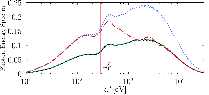
Figure 2: Energy spectra $dE_{Q}/d\omega^{\prime}$ (solid black line) and $\langle dE_{C}/d\omega^{\prime}\rangle$ (dash-dotted red line) for numerical parameters given in the text and the single-electron spectrum multiplied by two (dashed green line) and by four (dotted blue line).

As reference, we also show the single-electron spectra multiplied by two (dashed green line) and by four (dotted blue line), which are the same for the two electrons Angioi et al. (2016). Concerning the electrons, we have set $\bm{r}^{\prime}=(10^{-2},10^{-2},10^{-3})\,\text{eV}^{-1}\approx(2,2,0.2)\,\text{nm}$ and $\rho^{2}(\bm{p}^{\prime}_{j})/2\varepsilon^{\prime}_{j}$ to be a normalized Gaussian function, with average momentum $\bm{p}^{\prime}=(0,0,-10\,\text{MeV})$, transverse standard deviation $\sigma_{p^{\prime}_{\perp}}=\sigma_{p^{\prime}_{x}}=\sigma_{p^{\prime}_{y}}=31\,\text{eV}$ and longitudinal standard deviation $\sigma_{p^{\prime}_{\parallel}}=\sigma_{p^{\prime}_{z}}=0.62\,\text{eV}$. Concerning the plane wave, we have set $\omega=1.55\,\text{eV}$, $\mathcal{I}=10^{20}\,\text{W}/\text{cm}^{2}$, and $\psi_{L}(\phi)=\sin^{4}(\omega\phi/4)\sin(\omega\phi)$ for $0\leq\omega\phi\leq 4\pi$ and zero elsewhere, such that $\chi^{\prime}\approx 0.002$. Fig. 2 shows that the classical spectrum is coherent up to a given frequency, that can be calculated with Eq. (9); for this estimate we choose $\bm{n}^{\prime}\sim-(m\xi/2\varepsilon^{\prime},0,1)$, with $\xi=|e|\mathcal{E}/m\omega=5$, as a typical observation direction where the average radiated energy is large Mackenroth and Di Piazza (2011). We estimate the variations $\Delta\bm{p}^{\prime}_{\perp}$ and $\Delta\varepsilon^{\prime}\approx\Delta p^{\prime}_{\parallel}$ entering Eq. (9) via the standard deviations $\sigma_{p^{\prime}_{\perp}}$ and $\sigma_{p^{\prime}_{\parallel}}$, respectively. By also estimating $\varphi_{T}\sim 2\pi$ as the effective phase where the laser field is strong, we find from Eq. (9) that $\omega^{\prime}_{C}\approx 278\,\text{eV}$, in good agreement with Fig. 2 (see the red vertical line). The quantum spectrum (solid black line) is incoherent over the whole range shown in Fig. 2 because, by estimating $|\bm{k}^{\prime}_{\perp}|\sim\omega^{\prime}m\xi/\varepsilon^{\prime}$, we obtain that $\omega^{\prime}_{Q}\sim\min\{\sigma_{p^{\prime}_{\perp}}\varepsilon^{\prime}/m\xi,\sigma_{p^{\prime}_{\parallel}}\}$, which corresponds to $\omega^{\prime}_{Q}=\sigma_{p^{\prime}_{\parallel}}=0.62\,\text{eV}$. Thus, even if classical arguments would predict coherent emission until $\omega^{\prime}_{C}$, the lower bound $\omega^{\prime}_{Q}$ given by quantum mechanics, being orders of magnitude smaller, dominates. According to the estimations in the SM, the Coulomb repulsion between the two electrons before they enter the laser field can be neglected for the above numerical parameters.

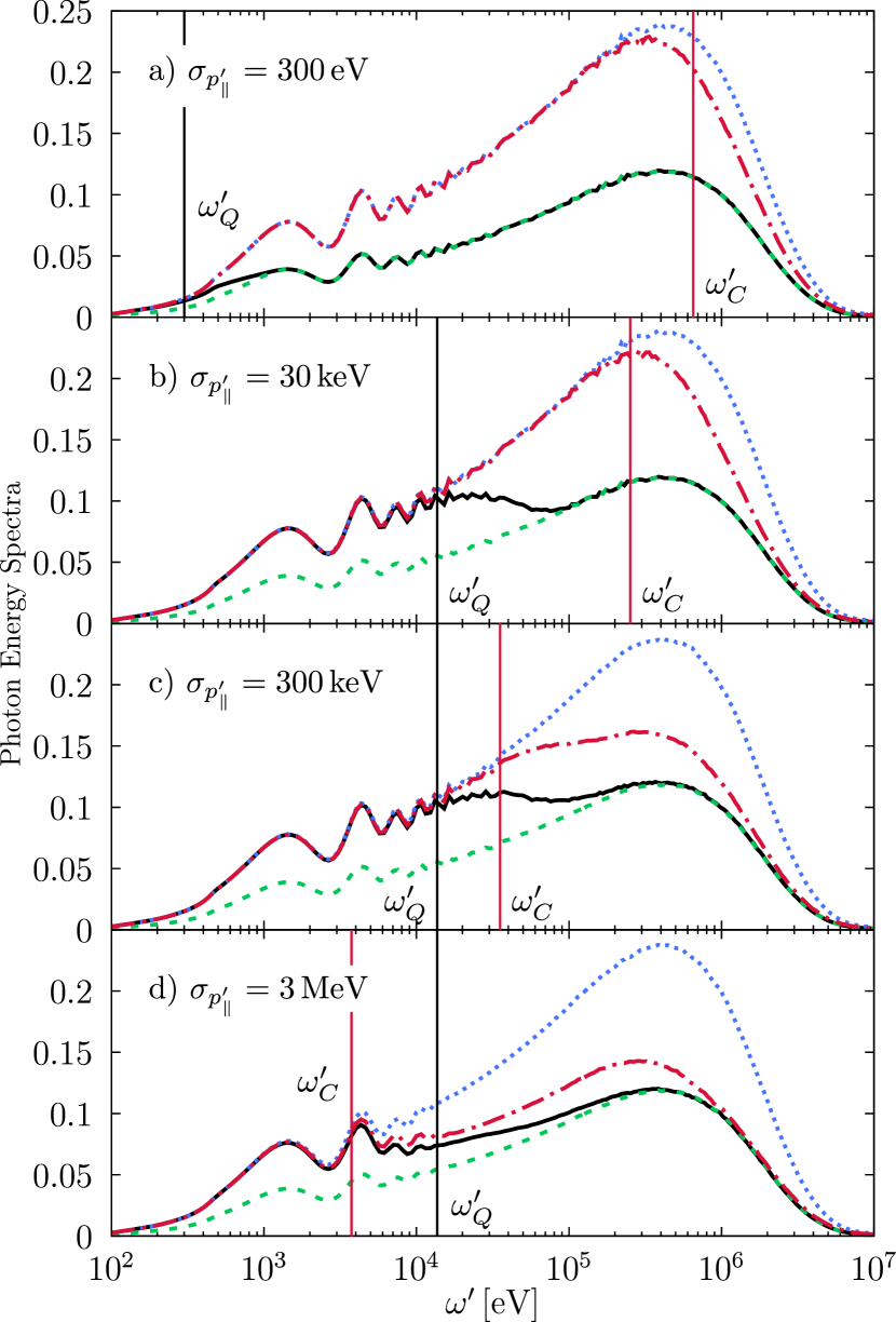
Figure 3: Energy spectra for numerical parameters given in the text. The meaning of each line is the same as Fig. 2.

In Fig. 3 we provide a compact visualization of the interplay between the classical and quantum limits on coherent emission. In order to show all the effects we mentioned in a single graph without changing multiple numerical parameters, we have fixed them at the same values of Fig. 2, except that $\bm{p}^{\prime}=(0,0,-100\,\text{MeV})$, $\sigma_{p^{\prime}_{\perp}}=1\,\text{keV}$, $\mathcal{I}=1.2\times 10^{21}\,\text{W}/\text{cm}^{2}$ ($\chi^{\prime}\approx 0.02$), $\bm{r}^{\prime}=(0,10^{-4},10^{-7})\,\text{eV}^{-1}$=(0,20,0.02) pm, and $\sigma_{p^{\prime}_{\parallel}}$ is varying in each panel. The largest difference between classical and quantum results is observed in panel a), where the Coulomb repulsion is not expected to play a significant role, whereas the latter may significantly alter the average distance between the electrons before they enter the laser field in the case of panels b)-d) (see the SM).

The values of $\omega^{\prime}_{Q}$, calculated in the same way as Fig. 2, and of $\omega^{\prime}_{C}$, estimated via Eq. (9), are in reasonable agreement with the numerical results. In particular, it is interesting to observe that the quantum limit dominates in panels a)-c), where $\omega^{\prime}_{C}>\omega^{\prime}_{Q}$, and the classical limit takes over in panel d) where $\omega^{\prime}_{C}<\omega^{\prime}_{Q}$, where it applies to both the classical and the quantum spectrum. We notice that in any case interference effects always amount to an increase of the radiation yield, an enhancement effect essentially due to the reduced distance between the two wave packets.

The properties of single-electron pulses with energies of the order of $0.1\,\text{MeV}$ and attosecond duration are already being exploited experimentally in order to perform high-precision microscopy (see Baum (2013); Kealhofer et al. (2016); Morimoto and Baum (2018a, b)), and control schemes for electrons of MeV energy have been demonstrated recently Curry et al. (2018). Moreover, recent theoretical studies indicate the feasibility of generating arbitrarily-delayed single-electron wave packets with GeV energies Krajewska et al. (2017). The extension of these techniques to few-electron wave packets seems possible Baum (2018), for instance by combining two single-electron pulses with the methods of Kealhofer et al. (2016); Morimoto and Baum (2018a, b) or via an ultracold gas source Claessens et al. (2005); van der Geer et al. (2009); Franssen et al. (2017), where the electrons are already highly correlated from the beginning. Our results suggest that the development of similar techniques at higher energies would have important applications also in fundamental strong-field physics. By reversing the argument, we can also say that the NSCS spectra as calculated here can be exploited, provided a detailed knowledge of the laser pulse, as a diagnostic tool for two- or few-electron high-energy pulses.

See pages 1,,,2,,3 of TE_SM.pdf