Negative Differential Mobility in Interacting Particle Systems

Abstract

Driven particles in presence of crowded environment, obstacles or kinetic constraints often exhibit negative differential mobility (NDM) due to their decreased dynamical activity. We propose a new mechanism for complex many-particle systems where slowing down of certain non-driven degrees of freedom by the external field can give rise to NDM. This phenomenon, resulting from inter-particle interactions, is illustrated in a pedagogical example of two interacting random walkers, one of which is biased by an external field while the same field only slows down the other keeping it unbiased. We also introduce and solve exactly the steady state of several driven diffusive systems, including a two species exclusion model, asymmetric misanthrope and zero-range processes, to show explicitly that this mechanism indeed leads to NDM.

The linear response of a system close to thermal equilibrium is characterized by the fluctuation-dissipation theorem Kubo . The current generated by a small external drive can be predicted from equilibrium correlation functions using the so-called Green-Kubo relations Green ; Kubo2 and the mobility, that is the ratio of the average particle current to the external force, remains necessarily positive. Away from equilibrium, the linear response formula gets modified Baiesi2009 and positivity of mobility is no longer guaranteed. In fact, particles driven far away from equilibrium might show absolute negative mobility anm1 ; anm2 ; anm3 ; anm4 or negative differential mobility.

Negative differential mobility (NDM) refers to the physical phenomenon when current in a driven system decreases as the external drive is increased zia ; rev . This has been observed in various systems, both in context of particle zia ; Barma ; Jack and thermal transport Li ; Hu ; deb . In particular, the occurrence of NDM of driven tracer particles in presence of obstacles Dhar ; neg ; neg2 ; Baiesi2015 ; Franosch or in steady laminar flow Sarracino2016 or crowded medium Saraccino ; Benichou2016 have been studied extensively in recent years. NDM has also been observed in driven many-particle systems in presence of kinetic constraints Sellitto or obstacles Baiesi2015 ; Reichhardt . The emergence of NDM in all these systems is typically associated with ‘trapping’ of the driven particles; the obstacles or the crowded environment slows down the particle motion as the driving is increased, which, in turn, reduces the current. This trapping is usually characterized by a decrease in the so called ‘traffic’ or dynamical activity neg ; neg2 , which plays a key role in understanding response of nonequilibrium systems Baiesi2009 ; Baiesi13 .

In interacting systems, current constitutes of contributions from many degrees of freedom (or different types of particles or modes), each of which can be driven separately; the external field might also act differently on different modes. Reducing the dynamical activity or ‘traffic’ of some degrees of freedom which are not necessarily driven, can be expected to influence the dynamical activity of the driven ones due to interaction; this raises a possibility of having a new mechanism to induce NDM in interacting systems.

In this article we propose a generic mechanism for NDM in driven interacting particle systems. We show that if the inter-particle interaction slows down the time scale of modes which are not necessarily driven, then a non-monotonic behaviour of current might arise leading to a negative differential mobility. We introduce an interacting two-species model to demonstrate explicitly that the increased external bias on one species can in fact reduce the dynamical activity of the other. NDM appears to be a direct consequence of this effect; trapping of driven particles alone by the increased bias may not be sufficient. To validate this scenario we introduce and study several exactly solvable models, the simplest being two distinguishable random walkers on a one dimensional lattice interacting via mutual exclusion. We explicitly show that when one of the particles is driven by an external field, corresponding current may decrease when the escape rate of the second, undriven, particle decreases as a function of the field. We generalize this scenario to interacting many particle systems with two or more species of particles, with and without hardcore interactions.

Let us first consider a system of interacting particles of two species on a one-dimensional periodic lattice of size $L.$ Each site $i=1,2\dots L$ is either vacant or occupied by at most one particle of kind $A$ or $B$, represented by the site variables $\tau_{i}=0,A,B$ respectively. The configuration of the system evolves following the dynamical rules,

$$A0\mathop{\rightleftharpoons}_{q}^{p}0A~{};~{}XB0\mathop{\rightarrow}^{r(X)}X0B~{};~{}0BX\mathop{\rightarrow}^{l(X)}B0X,$$ (1)

where $r(X),l(X)$ are the hop rates of a $B$ particle to the right and left empty neighboring sites, respectively, when $X=0,A,B$ is the occupancy of the other neighbor. Here we consider a specific case $q=1-p,$ $r(0)=w$ and all other rates $r(X)=1-w=l(X);$ this corresponds to the physical scenario where isolated B particles are driven by a constant bias quantified by $w$ while other $B$ particles diffuse symmetrically. In addition to the dynamics (1), we also allow an exchange between neighboring $A$ and $B$ particles,

$$AB\mathop{\rightleftharpoons}_{\alpha}^{\alpha}BA$$ (2)

to ensure ergodicity in the phase space. Clearly the dynamics conserves both densities $\rho_{A,B}=N_{A,B}/L$ where $N_{A,B}$ are the number of particles of the respective species. For a fixed value of parameters $w,\alpha$ and densities $\rho_{A,B}$ we would like to see how the current varies with $p$ or equivalently the biasing field $\varepsilon=\ln\frac{p}{1-p},$ defined consistently with local detailed balance kls , taking $k_{B}T=1$ for the sake of simplicity. Note that $B$ particles are not driven by this external field $\varepsilon.$

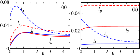
Figure 1: Current $j_{A,B}$ (solid line) and ‘traffic’ $i_{A,B}$ (dashed line), from simulations of the two species model defined in Eqs. (1) and (2) for $L=1000,\rho_{A}=0.1,$ $w=0.9$ and $\alpha=0.01.$ (a) and (b) correspond to $\rho_{B}=0.1,0.5$ respectively.

Using Monte Carlo simulations of the model we measure the average current $j_{A,B}=(\langle n_{r}^{A,B}\rangle-\langle n_{l}^{A,B}\rangle)/L$ where $\langle n_{r}^{A,B}\rangle$ ( $\langle n_{l}^{A,B}\rangle$) are the average number of right (left) jumps of $A$ or $B$ particles in unit time, measured in the steady state. Figure 1 shows $j_{A,B}$ for two different densities $\rho_{B}=0.1,0.5$ of the $B$-particles; NDM is seen in the former case while the current shows a monotonic behaviour in the latter one. To understand the origin of the NDM in this system and to investigate if the driving is, somehow, leading to a ‘trapping’ of the particles, we measure the average ‘traffic’ or time-symmetric current $i_{A,B}=(\langle n_{r}^{A,B}\rangle+\langle n_{l}^{A,B}\rangle)/L$ of the $A,B$ particles which are also shown in the Fig. 1 (dashed lines). The inverse of the traffic measures the typical time-scales associated with particle jumps; it seems that $i_{A}$ is a decreasing function of the drive signifying that the $A$ particles, apart from being driven, are indeed also ‘slowed down’ by the field $\varepsilon.$ Surprisingly, however, it turns out that, decreasing $i_{A}$ alone is not sufficient (see Fig. 1(b)) rather it is the slowing down of the $B$ particles which is the decisive factor giving rise to NDM note1 . To observe NDM, decreasing traffic of the driven degrees is certainly necessary (as observed in other many-particle systems Sellitto ; Baiesi2015 ) but its insufficiency here indicates presence of possible additional controlling factors.

Based on this phenomenological picture we propose a possible mechanism for NDM in interacting systems: particle current in a driven many particle system might show a non-monotonic behaviour if some modes, which are not driven by the external field, slow down with increased driving. To substantiate this scenario, we consider several interacting particle systems where some degrees of freedom are biased by the external field, whereas the same field slows down other modes explicitly. The aim is to show from exact steady state calculations that particle current in such situations indeed exhibit NDM, purely due to the effect of inter-particle interaction.

Two random walkers: As a simple prototypical example of two interacting current-carrying modes we consider two distinguishable particles, denoted by $A$ and $B,$ on a periodic lattice interacting via hardcore exclusion, i.e., the occupancy of the site $i$ is $\tau_{i}=A,B,0$ where particles $A$ and $B$ cannot occupy the same site. The particles follow a dynamics,

$$A0\mathop{\rightleftharpoons}_{q}^{p}0A,\quad B0\mathop{\rightleftharpoons}_{\psi}^{\psi}0B.$$ (3)

In this Two Random Walkers (TRW) model, the external bias affects the particles differently: the $A$ particle is driven by the external field $\varepsilon=\ln(p/q)$ whereas the $B$ particle performs an unbiased random walk with jump rate $\psi(\varepsilon)$ — also depending on the field $\varepsilon.$

We use the so called Matrix Product Ansatz MPAevans to express the steady state weight $P(C)$ for any configuration $C$ in a matrix product form : $P(C)=Tr[\prod_{i=1}^{L}X_{i}]$ where the matrix $X_{i}=\hat{A}\delta_{\tau_{i},A}+\hat{B}\delta_{\tau_{i},B}+\hat{E}\delta_{\tau_{i},0}$ represents occupancy $\tau_{i}$ of the site $i.$ The matrices $\hat{A},\hat{B},\hat{E}$ must satisfy the following set of algebraic relations to satisfy the Master equation in the steady state

$${\hat{A}}^{2}=0={\hat{B}}^{2};~{}p{\hat{A}}\hat{E}-q\hat{E}{\hat{A}}=x_{0}{\hat{A}};$$ (4)

$$\psi({\hat{B}}\hat{E}-\hat{E}{\hat{B}})=x_{0}{\hat{B}},$$ (5)

where $x_{0}$ is an auxiliary scalar. We find a $2\times 2$ representation of the matrices ${\hat{A}},{\hat{B}},\hat{E}$ which satisfies the algebra (5) with a choice $x_{0}=\psi\frac{p-q}{\psi+q},$

$$\begin{array}[]{ccc}{\hat{A}}=\left(\begin{array}[]{cc}0&1\\ 0&0\\ \end{array}\right)&{\hat{B}}=\left(\begin{array}[]{cc}0&0\\ 1&0\\ \end{array}\right)&\hat{E}=\left(\begin{array}[]{cc}\gamma&0\\ 0&1\\ \end{array}\right),\end{array}$$ (13)

where $\gamma=\frac{p+\psi}{q+\psi}.$ The partition function of the system of size $L$ is then $Z_{L}=\sum_{C}P(C)=Tr[({\hat{A}}+{\hat{B}}+\hat{E})^{L}]=\frac{\gamma^{L-1}-1}{\gamma-1}.$ The average stationary current of $A$ particle is

$$j_{A}=p\langle A0\rangle-q\langle 0A\rangle=x_{0}\frac{Z_{L-1}}{Z_{L}}\simeq\frac{(p-q)\psi}{(p+\psi)},$$ (14)

we have taken the thermodynamic limit $L\to\infty$ in the last step. Due to the presence of the interaction, the $B$ particle also exhibits a stationary current which depends on $\varepsilon;$ in fact, $j_{B}=j_{A}$ (as expected in the absence of particle exchange) and the total particle current $j=j_{A}+j_{B}=2\frac{(p-q)\psi}{(p+\psi)}.$ The response of the current $j$ to a small increase in $\varepsilon$ is quantified by the differential mobility

$$\frac{\textrm{d}j}{\textrm{d}\varepsilon}=\frac{(p^{\prime}-q^{\prime})\psi+(p-q)\psi^{\prime}}{(p+\psi)}-\frac{(p-q)\psi(p^{\prime}+\psi^{\prime})}{(p+\psi)^{2}},$$ (15)

where prime denotes derivative w.r.t. $\varepsilon.$ Equilibrium corresponds to $\varepsilon=0,$ i.e., $p=q$ (remember that $q=e^{-\varepsilon}p$) and the mobility, as expected near equilibrium, is positive irrespective of the functional form of $\psi.$ On the other hand, in the large driving limit $\varepsilon\to\infty,$ assuming $p$ and $p^{\prime}$ remain finite, we have,

$$j^{\prime}(\infty)=-\lim_{\varepsilon\to\infty}\frac{p^{2}\psi^{2}}{(p+\psi)^{2}}\frac{\textrm{d}}{\textrm{d}\varepsilon}\left(\frac{1}{p}+\frac{1}{\psi}\right)$$ (16)

This sets a criterion for NDM in TRW model: if asymptotically the increasing rate of $\psi^{-1}$ is larger than the decreasing rate of $p^{-1},$ then there will be a finite bias $\varepsilon^{*}>0$ above which the response is negative. Since the inverse rates measure the diffusion time scales, and the particles here interact via strong repulsive interaction (here hardcore), this criterion is in tune with the proposition given in Ref. Saraccino . In particular, for the cases $q=1/(1+e^{\varepsilon})$ (i.e., $p=1-q$) or $q=e^{-\varepsilon}$ ($p=1$), any choice of $\psi(\varepsilon)$ for which $\psi^{\prime}(\infty)<0$ would exhibit NDM. Current $j_{A}=j/2$ as a function of $\varepsilon$ for $q=e^{-\varepsilon},\psi(\varepsilon)=1/(1+\varepsilon)$ is shown in Fig. 2(a); NDM occurs here for $\varepsilon>\varepsilon^{*}=1.505.$

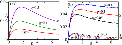
Figure 2: NDR in interacting two-species model. (a) $j_{A}$ obtained from exact steady state results for $\alpha=0$ are shown for $\rho_{B}=\rho_{A}=0.1,0.3;$ the threshold values are $\varepsilon^{*}=1.53,1.76$ respectively. For TRW model we plot $j_{A}/200$ for better visibility. (b) For $\alpha>0,$ $j_{A}$ (solid lines) and $j_{B}$ (dashed lines) are obtained from simulations with $L=1000,\rho_{A}=0.1,\rho_{B}=0.3,$ and different $\alpha=0.05,0.1$ and $0.15.$

A somewhat similar model with two coupled Brownian particles is studied in Ref. ac where only one of the particles was driven by both a static and a time-periodic force and it was observed that the second particle exhibits NDM in some parameter regime. In contrast, here we show that NDM occurs for both the particles when the escape rate of the undriven particle is decreased with increasing drive.

The TRW model, being a simple prototype of two current carrying modes, lacks some important features of realistic driven systems. In the following we study several more complex driven interacting systems and show that a similar mechanism indeed induces NDM.

Two species exclusion process: Our next example is a generalized version of dynamics (3) with an added particle exchange dynamics

$$A0\mathop{\rightleftharpoons}_{q}^{p}0A,\quad B0\mathop{\rightleftharpoons}_{\psi}^{\psi}0B,\quad AB\mathop{\rightleftharpoons}_{\alpha}^{\alpha}BA.$$ (17)

Unlike the TRW model, now we have macroscopic numbers of $A$ and $B$ particles, with conserved densities $\rho_{A}$ and $\rho_{B}$ respectively.

First let us consider the case $\alpha=0.$ In absence of particle exchange the number of $A$s ($B$s) trapped between to consecutive $B$s ($A$s) are conserved and thus the configuration space is not ergodic. One can however choose to work in one particular sector; the dynamics then enforces ergodicity within that sector. Let us work in a sector with exactly one A particle between two consecutive $B$s; the configurations are now $C\equiv\{A0^{n_{1}}B0^{n_{2}}A0^{n_{3}}B0^{n_{4}}\dots B0^{n_{2M}}\},$ each having exactly $N$ number of $A$s and $B$s, and $\sum_{i}n_{i}=L-2N$ number of vacancies. The steady state weights of this particular equal density ($\rho_{A}=\frac{N}{L}=\rho_{B}$) sector, can be obtained exactly using matrix product ansatz, by representing $A,B,0$ as matrices ${\hat{A}},{\hat{B}},{\hat{E}}$ respectively. The required matrix algebra in this case turns out to be same as Eq. (5) indicating Eq. (13) as a possible representation. However, unlike the TRW model, here we need to deal with finite densities $\rho_{A,B}.$ The grand canonical partition function is now $Z_{L}=Tr[(z{\hat{A}}+{\hat{B}}+{\hat{E}})^{L}]$ where $z$ is the fugacity associated with only A particles (additional fugacity for B particles is not needed as $\rho_{B}=\rho_{A}$). In the thermodynamic limit, $Z_{L}=\lambda_{+}(z)^{L}$ where $\lambda_{\pm}(z)=\frac{1}{2}(1+\gamma\pm\sqrt{(1-\gamma)^{2}+4z})$ are the eigenvalue of $(z{\hat{A}}+{\hat{B}}+\hat{E})$ and $\gamma=(p+\psi)/(q+\psi).$ This leads to $\rho_{A}=z\frac{\textrm{d}}{\textrm{d}z}\ln\lambda_{+}(z)=z/(\lambda_{+}^{2}-\lambda_{+}\lambda_{-}).$ The steady state current of $A$ particles is now

$$j_{A}=z(p\langle A0\rangle-q\langle 0A\rangle)=\frac{z(p-q\gamma)}{\lambda_{+}^{2}(\lambda_{+}-\lambda_{-})}$$ (18)

Explicit calculation shows that the current of $B$ particles $j_{B}=\psi(\langle B0\rangle-\langle 0B\rangle)$ is same as $j_{A}$ (as expected for $\alpha=0),$ thus $j=2j_{A}.$ The differential response $\frac{\textrm{d}j}{\textrm{d}\varepsilon}$ becomes negative as the field $\varepsilon$ is increased beyond some threshold $\varepsilon^{*},$ which depends on the densities $\rho_{A}=\rho_{B}$ as shown in Fig. 2(a) for $p=1,q=e^{-\varepsilon},$ and $\psi(\varepsilon)=1/(1+\varepsilon).$

For $\alpha>0,$ we do not have an exact solution; however, Monte Carlo simulation confirms that the model still exhibits NDM in a fairly large range of particle densities. Fig. 2(b) shows plots of $j_{A}$ and $j_{B}$ versus $\varepsilon$ for different values of $\alpha$ for $\rho_{A}=0.1,\rho_{B}=0.3.$

Asymmetric Misanthrope Process: It is interesting to ask whether it is possible to see NDM in systems without hardcore exclusion. To this end we investigate an asymmetric misanthrope process (AMP) AMP on a one-dimensional lattice where each site $i$ can hold any number of particles $n_{i}\geq 0.$ The particles can hop to their right or left nearest neighbors with a rate that depends on the occupation of both departure and arrival sites,

$$\{n_{i},n_{i+1}\}\mathop{\rightleftharpoons}^{u_{r}(n_{i},n_{i+1})}_{u_{l}(n_{i+1}+1,n_{i}-1)}\{n_{i}-1,n_{i+1}+1\};$$ (19)

the functional form of the rate functions $u_{r,l}(.),$ for right and left hops are different. This dynamics conserves density $\rho=\sum_{i}n_{i}/L.$ The asymmetric rate functions correspond to driving fields $E_{mn}=\ln\frac{u_{r}(m,n)}{u_{l}(n+1,m-1)}$ acting on bonds with local configurations $(m,n).$ Clearly, if $E_{mn}=0~{}~{}\forall~{}m,n,$ we have $u_{r}(m,n)=u_{l}(n+1,m-1)$ and the system is in equilibrium satisfying detailed balance condition with all configurations being equally likely.

We now choose a set of specific rate functions,

$$u_{r}(m,n)=\left\{\begin{array}[]{ll}\psi&n=0\\ 1&n>0\end{array}\right.;~{}u_{l}(m,n)=\left\{\begin{array}[]{ll}\psi&m=1\\ e^{-\varepsilon}&m>1,n=0\\ \frac{1}{2}&m>1,n>0\end{array}\right.,$$

which corresponds to

$$E_{mn}=\left[\ln 2+(\varepsilon-\ln 2)\delta_{m,1}\right](1-\delta_{n,0}).$$ (20)

Here, rightward hopping of particles to vacant neighbors are not biased (as both the rightward hop and corresponding reverse hop occur with same rate $\psi$) whereas other rightward jumps are biased by an external field which depends on the occupation of the departure site: $\varepsilon$ when the departure site has only one particle or otherwise a constant field $\ln 2$.

To explore the possibility of NDM in this system we did Monte Carlo simulation with $\psi(\varepsilon)=1/(1+\varepsilon).$ Figure 3(a) shows the particle current $j$ versus $\varepsilon$ (symbols) which depicts a non-monotonic behaviour; once again we see that slowing down a non-driven mode results in a NDM. This behaviour of current can be understood more rigorously from the exact steady state weights of AMP, which is of a factorized form $P(\{n_{i}\})\sim\prod_{i}f(n_{i}),$ when the rate functions satisfy certain conditions AMP . In the present case, these conditions require

$$\psi(\varepsilon)=\frac{2-e^{\varepsilon}+2\delta(1-e^{-\varepsilon})}{3e^{\varepsilon}-4}$$ (21)

with $\delta=\frac{1}{4}(e^{\varepsilon}-2+\sqrt{4+12e^{\varepsilon}+e^{2\varepsilon}})$, when $f(n)=\delta^{n-1}~{}\forall~{}n>0$ and $f(0)=1.$ Note that, this $\psi(\varepsilon)$ is still a decreasing function but the model is well defined only in the regime $\varepsilon>\ln\frac{4}{3}$ where $\psi>0.$ The grand canonical partition function is $Z_{L}=[F(z)]^{L}$ with $F(z)=\sum_{n}f(n)z^{n}=1+\frac{z}{1-\delta z},$ where fugacity $z$ controls the particle density through $\rho(z)=zF^{\prime}(z)/F(z)=z[(1-\delta z)(1+z-\delta z)]^{-1}.$ Finally, the current is,

$$j = \frac{1}{2[F(z)]^{2}}[(F(z)+2\psi-2e^{-\varepsilon}-1)(F(z)-1-z)$$ (23)

$$~{}~{}~{}~{}~{}~{}~{}~{}~{}~{}+2z(1-\psi)(F(z)-1)].$$

Fig. 3(a) shows $j$ as a function of $\varepsilon$ for density $\rho=0.15;$ NDM is observed for $\varepsilon\gtrsim 0.9$.

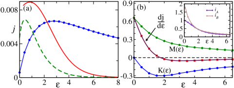
Figure 3: (a) Current $j$ versus $\varepsilon$ for AMP dynamics (20) for density $\rho=0.15.$ Circle: $\psi=1/(1+\varepsilon)$ (simulations), solid line: exact results for $\psi$ given by Eq. (21). Dashed line: current $j$ (multiplied by $0.01$ for better visibility) for AZRP dynamics (24). (b) Entropic and frenetic components of the linear response in the TRW model as a function of the driving $\varepsilon$ measured from Monte-Carlo simulations of a system of size $L=100.$ The inset shows the traffic $i_{A},i_{B}.$

The factorized steady state of AMP discussed above is also a steady state of the asymmetric zero range process (AZRP) for a class of rate functions AMP , one example being

$$u_{r}(n)=\frac{v(n)}{2}(2-v(n-1)),u_{l}(n)=v(n)-u_{r}(n)$$ (24)

where $v(n)=f(n-1)/f(n).$ We find that current in AZRP with above dynamics also exhibits NDM for large densities; see the dashed curve in Fig. 3(a). What appears essential for the occurrence of NDM is the asymmetric rate functions which, we think, can be realized experimentally with colloidal particles colloid in asymmetric separate channels sepChnl ; GeoAsym .

Nonequlibrium response relation: Away from equilibrium, the linear response of current $J$ can be expressed as a sum of two nonequilibrium correlations Baiesi2009 ,

$$\frac{\textrm{d}}{\textrm{d}\varepsilon}\langle J\rangle=\frac{1}{2}\left\langle S^{\prime}(\omega);J\right\rangle-\left\langle D^{\prime}(\omega);J\right\rangle.$$ (25)

where $S(\omega)$ and $D(\omega)$ are the entropy (anti-symmetric under time reversal) and ‘frenesy’ (symmetric) associated with a trajectory $\omega$ during time interval $[0,t];$ primes denote derivatives w.r.t $\varepsilon$ and $\langle f;g\rangle\equiv\langle fg\rangle-\langle f\rangle\langle g\rangle.$ For a single driven tracer, $S^{\prime}=J$ and the entropic term is simply the variance of the current while the frenetic one depends on the details of the specific dynamics. A large frenetic contribution which may occur, for example, in presence of traps or obstacles, can make the overall response negative neg ; neg2 . To understand how the entropic and frenetic components of mobility compete in systems where the escape rate (or the time-symmetric traffic) of the driven particle or mode is fixed whereas a non-driven mode is slowed down, let us consider the example of TRW model with $p+q=1.$ Since the driving is associated with the $A$ particle only, we have $S^{\prime}=J_{A},$ where $J_{A}$ is the time-integrated current of the $A$ particle during the time $[0,t].$ The change in dynamical activity is now,

$$D^{\prime}(\omega)=\frac{(p-q)}{2}I_{A}-\frac{\psi^{\prime}}{\psi}I_{B}-(p^{\prime}+\psi^{\prime})t_{AB}-(q^{\prime}+\psi^{\prime})t_{BA}$$

where $t_{AB}$($t_{BA}$) refers to the total time during which $B$ sits immediately to the right (left) of $A.$ For the stationary current $j=\lim_{t\to\infty}\langle J\rangle/t,$ the entropic component is then given by $M(\varepsilon)=\lim_{t\to\infty}\langle J_{A};J\rangle/2t$ and the frenetic component $K(\varepsilon)=-\lim_{t\to\infty}\langle D^{\prime}(\omega);J\rangle/t.$

Figure 3(b) shows plots of $M(\varepsilon)$ and $K(\varepsilon)$ obtained from Monte Carlo simulations. Similar to the single particle case, $M(\varepsilon)$ remains positive for all $\varepsilon>0$ whereas $K(\varepsilon)$ becomes negative resulting in NDM above a threshold field. The inset shows the average time-symmetric traffic $i_{A,B},$ both decrease as the driving is increased; the unbiased $B$ particle, being slowed down by the field $\varepsilon,$ in turn slows down the $A$ particle note2 .

Conclusion: In this article, we address the question of negative differential mobility (NDM) in interacting driven diffusive systems. It is known that NDM can occur when the driven particles are slowed down (increased time-scale of motion) by the external field. Here we propose an alternate mechanism and show that NDM can occur in multi-component system when the drive slows down some other, undriven, degree of freedom. First we illustrate this phenomenon in an exclusion process with two particle species where only one type of particles are driven by an external field. The other particles, although unaffected directly by the drive, slows down due to mutual interaction, resulting in NDM. To understand the mechanism we study a pedagogical example of two distinguishable random walkers on a periodic lattice interacting via exclusion only, one of which is driven by an external field. Other, more complex, exactly solvable examples of two-species exclusion process and asymmetric misanthrope process are also studied where the same mechanism leads to NDM for large driving. This mechanism provides a new direction to the occurrence of NDM in interacting particle systems, in contrast to the existing ones — jamming, kinetic constraints or trapping of driven modes.

References

- (1) R. Kubo, Rep. Prog. Phys. 29, 255 (1966).
- (2) M. S. Green, J. Chem. Phys. 22,398 (1954); Phys. Rev. 119, 829 (1960).
- (3) R. Kubo, J. Phys. Soc. Jpn. 12, 570 (1957).
- (4) M. Baiesi, C. Maes and B. Wynants, Phys. Rev. Lett. 103, 010602 (2009).
- (5) R. Eichhorn, P. Reimann, and P. Hänggi, Phys. Rev. Lett. 88, 190601 (2002).
- (6) A. Ros, R. Eichhorn, J. Regtmeier, T. T. Duong, P. Reimann and D. Anselmetti, Nature 436 928 (2005).
- (7) L. Machura, M. Kostur, P. Talkner, J. Łuczka, and P. Hänggi, Phys. Rev. Lett. 98, 040601 (2007).
- (8) P. K. Ghosh, P. Hänggi, F. Marchesoni, and F. Nori, Phys. Rev. E 89, 062115 (2014).
- (9) R. K. P. Zia, E. L. Præstgaard, and O.G. Mouritsen,Am. J. Phys. 70, 384 (2002).
- (10) R. Eichhorn, P. Reimann, B. Cleuren, and C. Van den Broeck, Chaos 15, 026113 (2005).
- (11) M. Barma and D. Dhar, J. Phys. C 16, 1451 (1983).
- (12) R. L. Jack, D. Kelsey, J. P. Garrahan, and D. Chandler, Phys. Rev. E 78, 011506 (2008).
- (13) B. Li, L. Wang, G. Casati, Appl. Phys. Lett. 88, 143501 (2006).
- (14) B. Hu, D. He, L. Yang, and Y. Zhang, Phys. Rev. E 74, 060101(R) (2006).
- (15) D. Bagchi, J. Phys.: Cond. Mat. 25, 496006 (2013).
- (16) P. Baerts, U. Basu, C. Maes, S. Safaverdi, Phys. Rev. E 88, 052109 (2013).
- (17) D. Dhar, J. Phys. A 17, L257 (1984).
- (18) S. Leitmann and T. Franosch, Phys. Rev. Lett. 111, 190603 (2013).
- (19) U. Basu and C. Maes, J. Phys. A: Math. Theor. 47, 255003 (2014).
- (20) M. Baiesi, A. L. Stella, and C. Vanderzande, Phys. Rev. E 92, 042121 (2015).
- (21) A. Sarracino, F. Cecconi, A. Puglisi, and A. Vulpiani, Phys. Rev. Lett. 117 174501 (2016).
- (22) O. Bénichou, P. Illien, G. Oshanin, A. Sarracino, and R. Voituriez, Phys. Rev. Lett. 113 268002 (2014).
- (23) O. Bénichou, P. Illien, G. Oshanin, A. Sarracino, and R. Voituriez, Phys. Rev. E 93, 032128(2016).
- (24) M. Sellitto, Phys. Rev. Lett. 101, 048301 (2008).
- (25) C. Reichhardt and C. J. O. Reichhardt, J. Phys.: Condens. Matter, in press (2017).
- (26) M. Baiesi, C. Maes, New J. Phys. 15, 013004 (2013).
- (27) S. Katz, J.L. Lebowitz, and H. Spohn, J. Stat. Phys. 34, 497 (1984).
- (28) We observe it for an extensive range of parameters; the data are not shown here.
- (29) R. A. Blythe, M. R. Evans, J. Phys. A Math. Theor. 40, R333 (2007).
- (30) M. Januszewski and J. Łuczka, Phys. Rev. E 83, 051117 (2011).
- (31) A. K. Chatterjee and P. K. Mohanty, J. Stat. Mech. 093201 (2017).
- (32) R. Eichhorn, J. Regtmeier, D. Anselmettib and P. Reimann, Soft Matter 6, 1858 (2010).
- (33) J. Wu and B. Ai, Sc. Rep. 6, 24001 (2016).
- (34) R. S. Shaw, N. Packard, M. Schroter, and H. L. Swinney, PNAS 104, 9580 (2007).
- (35) Note that, in absence of any interaction between and would be a constant since