Bragg-induced oscillations in non-$\mathcal{PT}$ complex photonic lattices

Abstract

When a monochromatic beam of light propagates through a periodic structure with the incident angle satisfying the Bragg condition, its Fourier spatial spectra oscillates between the resonant modes situated at the edges of the Brillouin zones of the lattice, exhibiting a nontrivial dynamics. Here, we investigate these Bragg-induced oscillations in a specific complex non-$\mathcal{PT}$ periodic structure, that is, a periodic medium with gain and loss with no symmetry under the combined action of parity and time reversal operations. We compare our analytic results based on the expansion of the optical field in Bragg-resonant plane waves with a direct numerical integration of the paraxial wave equation beyond the shallow potential approximation and using a wide Gaussian beam as initial condition. In particular, we study under which conditions a mode trapping phenomenon may still be observed and to inspect how the energy exchange between the spectral modes takes place during propagation in this more general class of asymmetric complex potentials.

I Introduction

The unified concept of Parity-Time ($\mathcal{PT}$) symmetry introduced by Bender and Boettcher almost twenty years ago is now part of an active area of scientific research bender1998real ; bender2007making ; bender1999pt ; bender2003must . Systems that are invariant under the combined action of parity and time symmetries can be described by non-Hermitian operators with a real-valued spectrum. A Hamiltonian operator is defined as $\mathcal{PT}$-symmetric if it commutes with the $\mathcal{PT}$ operator, $[\mathcal{PT},H]=0$. However, this condition alone does not guarantee that both commuting operators will share a common set of eigenvectors because the operator $\mathcal{T}$ is antilinear. In practice, the Hamiltonian $H(b)$ contains a free parameter $b$ which may be increased up to a critical value so that the system undergoes a symmetry breaking phase transition. When the symmetry of the Hamiltonian operator is broken, the commuting property does not guarantee any longer that the Hamiltonian and the $\mathcal{PT}$ operator share a common set of eigenvectors, and the Hamiltonian spectrum becomes fully or partially complex. In the physical context, $\mathcal{PT}$ symmetry behavior has been experimentally demonstrated in optical coupled waveguides makris2008beam ; guo2009observation ; ruter2010observation , silicon photonic circuits feng2011nonreciprocal , superconducting wires rubinstein2007bifurcation and even in classical mechanical systems bender2013observation , to cite a few.

Even though the concept of $\mathcal{PT}$ symmetry has increased the classes of possible physical Hamiltonians by extending Hermitian systems to the complex plane, such required symmetry is not sufficient or necessary for an operator to exhibit a real-valued spectrum. Although it can be shown that the eigenvalues of a $\mathcal{PT}$-symmetric Hamiltonian always show up as complex-conjugate pairs, this property is not exclusive to the $\mathcal{PT}$-symmetric systems. A necessary and sufficient condition for the spectrum of a non-Hermitian Hamiltonian to be purely real may be formulated in terms of a more general class of pseudo-Hermitian operators. It was shown extensively by Mostafazadeh, shortly after the seminal work of Bender and Boettcher, that Hamiltonians with $\mathcal{PT}$ symmetry are actually a subgroup of a more general class of pseudo-Hermitian Hamiltonians mostafazadeh2002pseudo ; mostafazadeh2002pseudo2 ; mostafazadeh2010pseudo ; mostafazadeh2004physical . In this theory, an operator $H$ is said to be $\eta$-pseudo-Hermitian if there exists a Hermitian invertible linear operator $\eta$ such that $H^{\dagger}=\eta H\eta^{-1}$. It was shown recently that it is possible to loosen the set of conditions on the pseudo-Hermiticity by requiring $\eta$ not to be invertible yang2017classes . We will discuss this new class of operators in section 2 below.

Optical beam oscillations induced by Bragg-resonance were studied ten years ago by Shchesnovich and Chávez-Cerda within the shallow potential approximation shchesnovich2007bragg . Bragg-induced Rabi oscillations is an allusion to the old Rabi problem, where matter oscillations between a two-level quantum system are driven by an external optical field, so that the authors named these optical oscillations driven by matter as well. However, we find more transparent and unambiguous to call these Bragg-induced oscillations simply Bragg oscillations. This is because there are other types of Rabi-like oscillations present in photonic systems makris2008optical ; trompeter2006bloch ; PhysRevLett.102.076802 . Bloch oscillations in an optical setup with $\mathcal{PT}$ symmetry was also considered longhi2009bloch . Until now, attention to Bragg oscillations in optical beams propagating in periodic photonic structures was devoted to linear Hermitian shchesnovich2007bragg , nonlinear Hermitian brandao2017effect , linear $\mathcal{PT}$-symmetric brandao2017bragg . It should be noted here, that in this last reference within a two-mode approach, oscillations were retrieved below the symmetry breaking point while above it, depending on the initial condition, exponential growth or mode trapping. In this paper, we consider a multimode approach of Bragg oscillations in a more general class of complex photonic lattices and retrieve the oscillations, with selected modes with higher amplitudes depending on the initial mode, and we also find unidirectional energy transference among modes when the optical medium presents a complex refractive index.

Section 2 is devoted to a discussion of non-$\mathcal{PT}$ potential operators and their spectra, where we show explicitly how one may tailor such potentials. We also introduce the periodic potential that is used throughout the paper. Section 3 presents the evolution equations for the spectral amplitudes of individual resonant plane waves as a first-order coupled system of differential equations. This system is solved by numerical techniques in section 4 along with its physical interpretation. Our conclusions are presented in section 5.

II Non-$\mathcal{PT}$ Hamiltonians

As pointed out in the last section, new classes of general non-$\mathcal{PT}$ symmetric potentials with arbitrary gain and loss regions were introduced cannata1998schrodinger ; miri2013supersymmetry ; tsoy2014stable ; nixon2016all ; yang2017classes . This is a huge step forward in the ability to construct arbitrary complex materials while still preserving a real spectrum of eigenvalues. We follow one such specific method for constructing arbitrary classes of complex materials that was introduced very recently yang2017classes . If $L=d^{2}/dx^{2}+V(x)$ is a Schrödinger operator and if there exists another operator $\eta$ such that $L$ and $\eta$ are related by a similarity relation

$$\eta L=L^{*}\eta,$$ (1)

then it is easy to show that all eigenvalues of $L$ appear in conjugate pairs if the kernel of $\eta$ is empty nixon2016all . This resembles the approach developed by Mostafazadeh mostafazadeh2002pseudo ; mostafazadeh2002pseudo2 but, in the present situation, $\eta$ need not be invertible. Given the generality of the $\eta$ operator, we choose it to be a combination of the parity operator $\mathcal{P}$ and differential operators as in

$$\eta=\mathcal{P}\left[\frac{d}{dx}+h(x)\right],$$ (2)

where $h(x)$ is a complex function whose properties we will now derive. When the right hand side of (1) acts on an arbitrary function $g(x)$ we have

$$\begin{split}L^{*}\eta g(x)&=-\frac{d^{3}g(-x)}{dx^{3}}+\frac{d^{2}[h(-x)g(-x)]}{dx^{2}}\\ &-V^{*}(x)\frac{dg(-x)}{dx}+V^{*}(x)h(-x)g(-x),\end{split}$$ (3)

while the left hand side of (1) reads

$$\begin{split}\eta Lg(x)&=-\frac{d^{3}g(-x)}{dx^{3}}-\frac{d[V(-x)g(-x)]}{dx}\\ &+h(-x)\frac{d^{2}g(-x)}{dx^{2}}+h(-x)V(-x)g(-x).\\ \end{split}$$ (4)

Since (1) must be satisfied, after letting $x\rightarrow-x$ and setting all coefficients of $g(x)$ and $dg(x)/dx$ equal to zero (because $\eta L-L^{*}\eta$ is the null operator), we have the following coupled system of differential equations

$$V(x)-V^{*}(-x)=2\frac{dh(x)}{dx},$$ (5)

and

$$[V(x)-V^{*}(-x)]h(x)=\frac{d^{2}h(x)}{dx^{2}}-\frac{dV(x)}{dx}.$$ (6)

After taking the complex conjugate of (5) together with the substitution $x\rightarrow-x$, it is easy to see that

$$-\frac{dh^{*}(-x)}{dx}=\frac{1}{2}[V^{*}(-x)-V(x)]=-\frac{dh(x)}{dx},$$ (7)

which follows that $dh^{*}(-x)/dx=dh(x)/dx$ and, after integrating both sides, $h^{*}(-x)=h(x)+c_{1}$ with $c_{1}$ being the constant of integration. Next, let us substitute the right hand side of (5) into the left hand side of (6) to obtain

$$2h(x)\frac{dh(x)}{dx}=\frac{d^{2}h(x)}{dx^{2}}-\frac{dV(x)}{dx},$$ (8)

and, after integrating once,

$$\int^{h(x)}2hdh=\int^{\frac{dh}{dx}}d\left(\frac{dh}{dx^{\prime}}\right)-\int^{V(x)}dV+c_{2},$$ (9)

where $c_{2}$ groups all constants of integration. It is then easy to see that $V(x)$ is given by

$$V(x)=\frac{dh(x)}{dx}-h^{2}(x)+c_{2}.$$ (10)

Since $c_{2}$ only adds a constant value to the potential function, we may, without loss of generality, choose it as $c_{2}=0$. To find the value of $c_{1}$ we substitute (10) and the expression $h^{*}(-x)=h(x)+c_{1}$ into (5)

$$c_{1}[2h(x)+c_{1}]=0.$$ (11)

Therefore, we can choose $c_{1}=0$. Since now $h^{*}(-x)=h(x)$ it follows that the function $h(x)$ is $\mathcal{PT}$-symmetric. So, by choosing a $\mathcal{PT}$-invariant function $h(x)$ one may generate the potential function

$$V(x)=\frac{dh(x)}{dx}-h^{2}(x).$$ (12)

The choice of the $\mathcal{PT}$-symmetric $h(x)$ function is completely arbitrary and, to study a periodic potential, we follow yang2017classes in choosing the convenient expression $h(x)=1+\cos x+ib\sin x$, with $b$ as a free real and positive parameter. The potential is then given explicitly by

$$V(x)=b^{2}\sin^{2}x-\cos^{2}x-\sin x-2\cos x-1\\ +ib[\cos x-2\sin x-\sin(2x)],$$ (13)

that is, a potential complex function whose real and imaginary parts are not even and odd respectively, and it is a periodic function with period $2\pi$. Nevertheless, the spectrum of (13) is completely real for $b<1$ and partially complex for $b>1$ as shown in yang2017classes . Therefore, this is an explicit example of a potential that is not $\mathcal{PT}$-symmetric and yet has a phase transition point. In the next section, we will address the problem of light propagation through an asymmetric potential function as given in (13). In particular, we will be interested in the evolution of the Bragg modes when the lattice is at the breaking point $b=1$.

III Evolution equations

We will assume from now on that the propagation of monochromatic scalar optical beams $\psi(x,z)$ is well described by the dimensionless (1+1)-dimensional paraxial wave equation

$$i\psi_{z}=-\psi_{xx}+V(x)\psi,$$ (14)

where $z$ is the propagation distance, $x$ the transverse coordinate and $V(x)$ is the potential (13) representing the properties of the photonic lattice. Before we discuss the ansatz used to solve (14) we decompose the potential $V(x)$ into its harmonic components

$$V(x)=\sum_{n=-\infty}^{\infty}V_{n}e^{inx}$$ (15)

where the, generally complex, Fourier amplitudes of the potential are given by $V_{-2}=-(1/4)(1-b)^{2}$, $V_{-1}=-(i/2+1)(1-b)$, $V_{0}=-[1+(1-b^{2})/2]$, $V_{1}=(i/2-1)(1+b)$ and $V_{2}=-(1/4)(1+b)^{2}$. The fact that some Fourier amplitudes are complex numbers is a clear signature of the non-$\mathcal{PT}$ nature of the potential considering that, for $\mathcal{PT}$-symmetric potentials, $V(x)=\sum_{n}V_{n}e^{inx}=\sum_{n}V_{n}^{*}e^{inx}=V^{*}(-x)$, and thus $V_{n}\in\mathbb{R}$.

Since it is known that only resonant Bragg modes are coupled during propagation when the incident beam is wide shchesnovich2007bragg ; brandao2017bragg ; brandao2017effect , we choose the ansatz to be

$$\psi(x,z)=\sum_{n=0,\pm 1,\pm 2,...}\psi_{n}(z)\exp(inx),$$ (16)

where $\psi_{n}(z)$ represents the spectral amplitude of mode $n$ at a distance $z$. After substituting expressions (15) and (16) into the paraxial wave equation (14) we arrive at the following set of coupled first order differential equations for the spectral amplitudes $\psi_{n}(z)$:

$$i\frac{d\psi_{n}}{dz}=(n^{2}+V_{0})\psi_{n}+V_{-2}\psi_{n+2}\\ +V_{-1}\psi_{n+1}+V_{1}\psi_{n-1}+V_{2}\psi_{n-2}.$$ (17)

We will also be interested in the power as a function of $z$, which can be calculated directly from the field $\psi(x,z)$ or as an incoherent sum of all spectral amplitudes $\psi_{n}(z)$:

$$P(z)=\int_{-\infty}^{\infty}|\psi(x,z)|^{2}dx=\sum_{n=0,\pm 1,\pm 2,...}|\psi_{n}(z)|^{2}.$$ (18)

The second equal sign used in relation (18) is not strictly correct since plane waves have infinite energy, so the right-hand side of this equation should be viewed as energy per unit (transverse) length. The general outline for the rest of the paper is to solve system (17), by considering a finite number of modes, subjected to initial conditions and to determine its power and Fourier spectra evolution.

IV Numerical results and discussion

Let us assume that only eleven modes are coupled through relation (17): $n\in\{\pm 5,\pm 4,\pm 3,\pm 2,\pm 1,0\}$. Within this approximation, the system (17) may be solved numerically after specifying the initial conditions for the eleven spectral amplitudes $\psi_{n}(0)$. Let us consider the lattice at the symmetry breaking point, $b=1$, and that only mode $n=0$ is initially populated, $\psi_{0}(0)=1$, with all others modes, $\psi_{n}(0)=0$ . Figure 1 shows the power evolution, $P(z)=\sum_{n}|\psi_{n}(z)|^{2}$, calculated in terms of the spectral amplitudes, along with the power evolution, $P(z)=\int|\psi(x,z)|^{2}dx$, calculated from the numerical solution of (14) with a Gaussian beam as initial condition, given by

$$\psi(x,0)=\exp\left[-\frac{1}{2}\left(\frac{x}{W}\right)^{2}\right],$$ (19)

where $W$ is the initial beam width. Part (a) of Figure 1 depicts the power evolution with $W=10$ and parts (b) and (c) with $W=25$ and $W=50$, respectively. One may conclude from Figure 1 that our approximation describes better the power evolution for wider initial beams and therefore one should expect this finite-width beam approach to corroborate the results obtained by the plane wave approach. Also, by closely inspecting the profiles shown in Figure 1, one may note that the power evolution is not exactly a sine or a cosine function due to the appearance of some relatively small bumps between the maximum and minimum points. Until now, to the best of our knowledge, no explanation or study has been given to the physical mechanism behind such specific behavior of the power evolution. However, this behavior may be understood, by examining the dynamics involved in the excitation of the Bragg-modes of the wavefield, as we now show. Figure 2 depicts the excited Fourier modes {$\psi_{0}$, $\psi_{1}$, $\psi_{2}$, $\psi_{3}$} during propagation. The modes with $n$ negative are exactly zero for this particular set of parameters and the modes {$\psi_{4}$, $\psi_{5}$} are negligible on the scale that is shown in Figure 1 and are therefore suppressed. Surprisingly, mode $\psi_{0}$ is trapped at $k=0$, in the sense that its spectral energy does not change during propagation. On the other hand, the modes $\psi_{1}$, $\psi_{2}$ and $\psi_{3}$ experience power oscillations shchesnovich2007bragg ; brandao2017bragg . One may now conclude, that the small bumps appearing in Figure 1 are mainly due to the excited Bragg mode $\psi_{2}$, as shown in Figure 2. One may note that the sum of the four curves in this plot is equal to the resultant continuous curve for the power evolution shown in Figure 1. This is to be expected according to relation (18). Since only modes with $n\geq 0$ are excited in this scenario, we expect the beam to propagate in the positive direction of the $x$ axis. This is seen in Figure 3 where the intensity, $|\psi(x,z)|^{2}$, of the Gaussian beam with $W=50$ is shown. By comparing Figures 1 and 3, it can be seen that the points of minimum value in the power evolution can be correlated to the minimum values of the intensity, as expected.

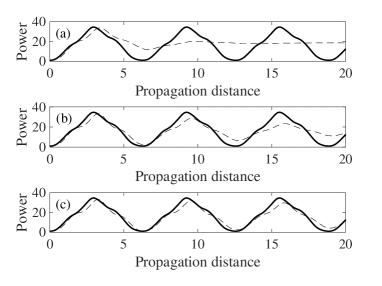
Figure 1: Power evolution in a non-$\mathcal{PT}$- symmetrical complex lattice defined in (13). Continuous lines represent the solutions of (17). Dashed lines are plotted from the numerical solution of the paraxial wave equation with a Gaussian input of the form $\psi(x,0)=\exp[-(x/W)^{2}]$ with (a) $W=10$, (b) $W=25$ and (c) $W=50$.

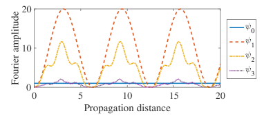
Figure 2: Evolution of the Fourier amplitudes $|\psi_{n}(z)|^{2}$ for $n=0,1,2$ and 3, corresponding to the parameters of Figure 1.

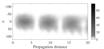
Figure 3: Intensity evolution in the $(x,z)$ plane for a Gaussian beam propagating through the lattice (13) with $W=50$. The regions where the intensity is a minimum are related by the power evolution of Figure 1.

Next, we consider the spectral component $\psi_{1}$ to be initially populated, $\psi_{1}(0)=1$, and all others empty. The evolution of the spectral amplitudes $\psi_{1}$, $\psi_{2}$ and $\psi_{3}$ is shown in Figure 4(a), after numerically solving the system (17). The other eight spectral components are either zero or negligible on the scale of the plot and are, therefore, not shown. Once more, the initially populated amplitude is trapped during propagation. On the other hand, the Bragg modes $\psi_{2}$ and $\psi_{3}$ undergo periodic Rabi-like oscillations and are therefore continuously exchanging energy with the medium. The amplitude of oscillation of mode $\psi_{2}$ is approximately two times the amplitude of mode $\psi_{1}$. Part (b) of Figure 4 depicts the power evolution for these parameters illustrating a very close agreement between the model (16) represented by the continuous line, and the simulation of an initial Gaussian beam $\psi(x,0)=\exp\left[-(1/2)\left(x/W\right)^{2}\right]\exp(ix)$ centered at $k=1$, represented by the dashed line. The power oscillates in a more sinusoidal form than the previous situation presented in Figure 1. Figure 4(c) depicts the intensity evolution $|\psi(x,z)|^{2}$ for $W=50$. As only positive Bragg modes are excited, the beam has a tendency to travel to the right, as expected. Comparing the intensity evolution displayed in part (c) with the power evolution in part (b), one finds that the beam exchanges much less energy from the medium compared to Figure 1. This is due to the fact that the spectral component $\psi_{2}$ oscillates with a much smaller amplitude than the spectral component $\psi_{1}$ as one may note from Figure 2.

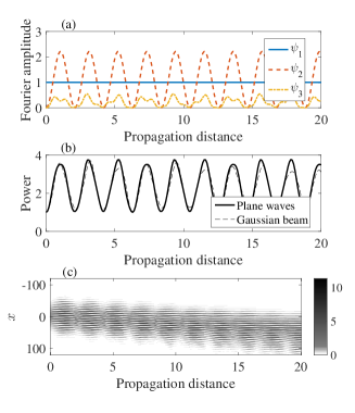
Figure 4: (a) Spectral amplitudes evolution with $\psi_{1}(0)=1$ and all other $\psi_{n}(0)=0$ of the lattice corresponding to Figures 1-3. (b) Power evolution calculated from the spectral amplitudes (solid line) and from the Gaussian beam (dashed line). (c) Intensity in the $(x,z)$ plane for the Gaussian beam with $W=50$.

Now let us address one of the situations considered in yang2017classes where the mode $\psi_{2}$ is initially populated. Figure 5 shows the results of the numerical simulations involving plane waves and a Gaussian beam given by $\psi(x,0)=\exp\left[-(1/2)\left(x/W\right)^{2}\right]\exp(2ix)$ to match the initially populated mode $\psi_{2}$. Once more, the energy of the initially populated spectral mode is trapped, as can be seen in part (a) of Figure 5. But in this situation, besides the $\psi_{2}$, only mode $\psi_{3}$ contributes to the evolution of the beam by oscillating Rabi-like during propagation, as the yellow color line in Figure 5(a) shows. From previous discussions, we conclude that the Bragg contributions to the power evolution are given by a constant function and an oscillatory one with peculiar features stemming from the simultaneous excitation of various modes: the initial input mode (say mode $\psi_{n}$), for which $\psi_{n}(0)=1$ becomes trapped with constant amplitude while the right-handed neighboring mode $\psi_{n+1}$, for which $\psi_{n+1}(0)=0$ is supplied with a larger portion of energy from matter. Part (b) of Figure 5 shows the power evolution from the Bragg modes (continuous line) compared to the Gaussian beam power (dashed line). The agreement between the two approaches seems to be very good. Since only two modes are excited during propagation, $\psi_{2}$ and $\psi_{3}$, we expect the beam to propagate mainly toward the positive $x$ direction. This can be verified by inspecting Figure 5(c) where the intensity evolution for a Gaussian beam with $W=50$ is shown and is clearly unidirectional.

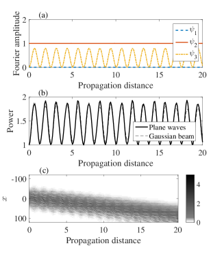
Figure 5: (a) Spectral amplitudes evolution with $\psi_{2}(0)=1$ and all other $\psi_{n}(0)=0$, of the lattice corresponding to Figures 1-3. (b) Power evolution calculated from the spectral amplitudes (solid line) and from the Gaussian beam (dashed line). (c) Intensity in the $(x,z)$ plane for the Gaussian beam with $W=50$.

The existence of a pure trapped Bragg mode, as predicted in brandao2017bragg for $\mathcal{PT}$-symmetric lattices seems to be very rare and probably only achievable within the shallow potential approximation. So, even though the intensity pattern depicted in Figure 5(c) suggests a transparent medium, there is another excited Bragg mode and, therefore, visible to the lattice, which reflects the field even with the lattice at the symmetry breaking point $b=1$. We are now in a position to discuss an incident beam that excites Bragg modes with $n$ negative. However, as demonstrated for $\mathcal{PT}$-symmetric lattices brandao2017bragg , when the photonic lattice is at the symmetry breaking point and the initial input power is totally in $k=-1$, the Bragg modes continuously absorb energy and diverge during propagation. Therefore, we expect our eleven-modes approach to become invalid for this regime, at least when $z$ is large. To verify these claims, we present in Figure 6 the spectral evolution for a wavefield whose spectral amplitude $\psi_{-1}(0)=1$ is initially populated while all others are zero. We clearly see that the amplitudes {$\psi_{1}$,$\psi_{2}$,$\psi_{3}$} grow indefinitely compared to the others. This implies that the medium is continuously giving energy to the field which becomes unbounded in amplitude. Figure 6(b) shows the power evolution predicted by (17) and we conclude that it describes very well the power evolution when compared to a Gaussian beam $\psi(x,0)=\exp\left[-(1/2)\left(x/W\right)^{2}\right]\exp(-ix)$ with $W=50$. Some other nonzero spectral amplitudes are shown in Figure 7 where, surprisingly, we see that the spectral amplitude $\psi_{0}$ does not grow indefinitely during propagation. It reproduces a pure Rabi-like profile exchanging energy periodically with the medium. This is a remarkable result as one finds that a stable Fourier amplitude oscillation is achieved in this unusual configuration, that is, at the critical point of a complex non-$\mathcal{PT}$ optical lattice. Note that the coupling, in all cases, depends strongly on the initial conditions: the initial mode, say $\psi_{n}$, always become trapped while the mode $\psi_{n+1}$ becomes strongly coupled as in the previous cases.

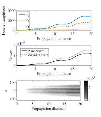
Figure 6: (a) Spectral amplitudes evolution with $\psi_{-1}(0)=1$ and $\psi_{n}(0)=0$ for the lattice corresponding to Figures 1-3. (b) Power evolution calculated from the spectral amplitudes (solid line) and from the Gaussian beam (dashed line). (c) Intensity in the $(x,z)$ plane for the Gaussian beam with $W=50$.

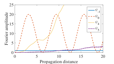
Figure 7: Fourier amplitude evolution for four modes corresponding to the system in Figure 6. One can clearly see that mode $\psi_{0}(z)$ is stable and oscillates in a Rabi-like fashion even though the beam is incident in the negative $x$ direction.

V Conclusions

We have studied Bragg oscillations in a non-$\mathcal{PT}$-symmetric complex photonic lattice. We find rich dynamics with asymmetric energy exchange between Bragg modes during the propagation of an optical field. Depending on the incident angle, Rabi-like oscillations are indeed achievable in complex photonic lattices, at the critical point. Power oscillations exhibit peculiar features stemming from the excitation of several modes, besides the initial one. The trapping of a pure Bragg mode with a non-vanishing amplitude in the more general context of a lattice was not observable. We have also found evidence of stable Fourier spectra evolution even when the incident input power is concentrated in $\psi_{n}$ with $n<0$ , which means, a beam travelling in the negative $x$ direction. These are unusual features: a stable Fourier amplitude evolution that persists even with negative $n$ and particularly at the critical point, where the Hamiltonian spectrum becomes partially complex. It should be noted here that, in spite of the simple model used here, we have been able to compare its results with numerical ones and shown that the former are quite reliable. Due to its relative simplicity, we hope that the present model might offer insights into the study of systems described by a complex photonic lattice described by a non-Hermitian complex index of refraction. The extension of optical systems to the complex plane should well open up the way to a new generation of optical devices and techniques useful in the pursue of the control of light.

References

- (1) C. M. Bender, S. Boettcher, Physical Review Letters 80, 5243 (1998).
- (2) C. M. Bender, Rep. Prog. Phys. 70, 947 (2007).
- (3) C. M. Bender, S. Boettcher, P. N. Meisinger, J. of Mat. Phys. 40, 2201 (1999).
- (4) C. M. Bender, D. C. Brody, . H. F. Jones, Am. J. Phys. 71, 1095 (2003).
- (5) K. G. Makris, R. El-Ganainy, D. Christodoulides, Z. H. Musslimani, Phys. Rev. Lett. 100, 103904 (2008).
- (6) A. Guo, G. Salamo, D. Duchesne, R. Morandotti, M. Volatier-Ravat, V. Aimez, F. Siviloglou, D. Christodoulides, Phys. Rev. Lett. 103, 093902 (2009).
- (7) C. E. Rüter, K. G. Makris, R. El-Ganainy,D. N. Christodoulides, M. Segev, D. Kip, Nat. Phys. 6, 192 (2010).
- (8) L. Feng, M. Ayache, J. Huang, Y.-L. Xu, M.-H. Lu, Y.-F. Chen, Y. Fainman, A. Scherer, Science 333, 729 (2011).
- (9) J. Rubinstein, P. Sternberg, Q. Ma, Phys. Rev. Lett. 99, 167003 (2007).
- (10) C. M. Bender, B. K. Berntson, D. Parker, E. Samuel, Am. J. Phys. 81, 173 (2013).
- (11) A. Mostafazadeh, J. of Math. Phys. 43, 205 (2002).
- (12) A. Mostafazadeh, J. of Math. Phys. 43, 2814 (2002).
- (13) A. Mostafazadeh, Int. J. of Geom. Meth. in Mod. Phys. 7, 1191 (2010).
- (14) A. Mostafazadeh, A. Batal, J. of Phys. A: Math. and Gen. 37, 11645 (2004).
- (15) J. Yang, Opt. Lett. 42, 4067 (2017).
- (16) V. S. Shchesnovich, S. Chávez-Cerda, Opt. Lett. 32, 1920 (2007).
- (17) K. Makris, D. Christodoulides, O. Peleg, M. Segev, D. Kip, Opt. Exp. 16, 10309 (2008).
- (18) H. Trompeter, W. Krolikowski, D. N. Neshev, A. S. Desyatnikov, A. A. Sukhorukov, Y. S. Kivshar,T. Pertsch, U. Peschel, F. Lederer, Phys. Rev. Lett., 96, 053903 (2006).
- (19) F. Dreisow, A. Szameit, M. Heinrich, T. Pertsch, S. Nolte, A. Tünnermann, S. Longhi, Phys. Rev. Lett. 102, 076802 (2009).
- (20) S. Longhi, Phys. Rev. Lett. 103 (2009).
- (21) P. A. Brandão, S. B. Cavalcanti, Phys. Rev. A 96, 053841 (2017).
- (22) P. A. Brandão, S. B. Cavalcanti, Opt. Commun. 400, 34 (2017).
- (23) F. Cannata, G. Junker, J. Trost, Phys. Lett. A 246, 219 (1998).
- (24) M.-A. Miri, M. Heinrich, D. N. Christodoulides, Phys. Rev. A 87, 043819 (2013).
- (25) E. N. Tsoy, I. M. Allayarov, F. K. Abdullaev, Opt. Lett. 39, 4215 (2014).
- (26) S. Nixon, J. Yang, Phys. Rev. A 93, 031802 (2016).