Holographic Four-Point Functions in the $(2,0)$ Theory

Abstract

We revisit the calculation of holographic correlators for eleven-dimensional supergravity on $AdS_{7}\times S^{4}$. Our methods rely entirely on symmetry and eschew detailed knowledge of the supergravity effective action. By an extension of the position space approach developed in Rastelli:2016nze ; longads5 for the $AdS_{5}\times S^{5}$ background, we compute four-point correlators of one-half BPS operators for identical weights $k=2,3,4$. The $k=2$ case corresponds to the four-point function of the stress-tensor multiplet, which was already known, while the other two cases are new. We also translate the problem in Mellin space, where the solution of the superconformal Ward identity takes a surprisingly simple form. We formulate an algebraic problem, whose (conjecturally unique) solution corresponds to the general one-half BPS four-point function.

1 Introduction

Correlation functions of local operators in holographic CFTs were among the first observables to be computed using the AdS/CFT dictionary, but only recently Rastelli:2016nze ; longads5 efficient calculational methods have begun to be developed. The traditional recipe is based on a perturbative expansion in Witten diagrams, which becomes very cumbersome (already at tree level) for $n$-point correlators with $n\geqslant 4$. Prior to our work, only a few four-point correlators of Kaluza-Klein (KK) modes were known, to wit (focussing for definiteness on the maximally supersymmetric backgrounds): a handful of cases in the $AdS_{5}\times S^{5}$ background Freedman:1998bj ; Arutyunov:2000py ; Arutyunov:2002fh ; Arutyunov:2003ae ; Berdichevsky:2007xd ; Uruchurtu:2008kp ; Uruchurtu:2011wh ; just the four-point function of the lowest KK mode (the stress-tensor multiplet) in the $AdS_{7}\times S^{4}$ background Arutyunov:2002ff ; and no results whatsoever in the $AdS_{4}\times S^{7}$ background.

The traditional method has two sources of computational complexity: the need for explicit expressions of the vertices in the supergravity effective action; and the proliferation of exchange Witten diagrams as the KK level is increased. In Rastelli:2016nze ; longads5 we introduced new calculational tools to circumvent these difficulties, for the case of $AdS_{5}\times S^{5}$ supergravity. A first approach, which we refer to as the “position space method”, leverages the special feature of the $AdS_{5}\times S^{5}$ background that all exchange Witten diagrams can be written as finite sums of contact diagrams. One can then write an ansatz for the four-point correlator as a sum of contact diagrams, and determine their relative coefficients by imposing superconformal symmetry, with no need for a detailed knowledge of the effective supergravity action. While simpler than the standard perturbative recipe, the position space method also quickly runs out of steam as the KK level is increased. What’s worse, the answer takes a completely unintuitive form, with no simpe general pattern. The second, more powerful approach of Rastelli:2016nze ; longads5 uses the Mellin representation of conformal correlators Mack:2009mi ; Penedones:2010ue . Tree-level holographic correlators in $AdS_{5}\times S^{5}$ are rational functions of Mandelstam-like invariants, with poles and residues controlled by OPE factorization, in close analogy with tree-level flat space scattering amplitudes. Superconformal symmetry is made manifest by solving the superconformal Ward identity in terms of an “auxiliary” Mellin amplitude. The consistency conditions that this amplitude must satisfy define a very constrained algebraic problem, which very plausibly admits a unique solution. While the position space method is implemented on a case-by-case basis for different correlators, the Mellin algebraic problem takes a universal form. We were able to solve the problem in one fell swoop for all half-BPS four-point function with arbitrary weights – a feat extremely difficult to replicate in position space.

The goal of this note is to extend these techniques to eleven-dimensional supergravity on $AdS_{7}\times S^{4}$. This is a background of extraordinary physical interest, as it provides a dual description of the mysterious six-dimensional $(2,0)$ theory at large $n$, and a prime target for our methods, since we expect maximal supersymmetry to constrain the tree-level holographic correlators uniquely. At a more technical level, this background enjoys the same “truncation conditions” as $AdS_{5}\times S^{5}$, such that exchange Witten diagrams can be written as finite sums of contact diagrams – equivalently, tree-level Mellin amplitudes are rational functions of the Mandelstam invariants. By contrast, the truncation conditions do not hold for the $AdS_{4}\times S^{7}$ background, and new tools are needed Zhou .

In this paper we focus on four-point functions of identical one-half BPS local operators,

$$\langle\mathcal{O}^{(k)}(x_{1})\mathcal{O}^{(k)}(x_{2})\mathcal{O}^{(k)}(x_{3})\mathcal{O}^{(k)}(x_{4})\rangle\;.$$ (1)

The operator $\mathcal{O}^{(k)}$ is the superconformal primary of the short multiplet $\mathcal{D}\big{(}2k;0,0,0;0,k\big{)}$. It has conformal dimension $\Delta=2k$ and transforms in the symmetric traceless representation of the R-symmetry group $SO(5)\cong USp(4)$. The integer $k\geqslant 2$ corresponds to the Kaluza-Klein level on the supergravity side. In particular $\mathcal{O}^{(2)}$ is the superprimary of the stress tensor multiplet, whose four-point function has been computed by Arutyunov and Sokatchev Arutyunov:2002ff , while operators with $k\geqslant 3$ are dual to massive Kaluza-Klein modes. No four-point functions for massive KK modes have ever been computed, partly because of the extraordinary challenge of evaluating the quartic vertices of the $AdS_{7}$ effective action from the non-linear KK reduction.

The position space method of Rastelli:2016nze ; longads5 admits a straightforward extension to the $AdS_{7}\times S^{4}$ background. Using this method we confirm the result of Arutyunov:2002ff for the stress-tensor multiplet four-point function and obtain two new explicit cases with KK levels $k=3$ and $k=4$. An important test of our results is that they are compatible with the expected chiral algebra structure identified in Beem:2013sza ; Beem:2014kka . By performing a certain “twist” that identifies spacetime and R-symmetry cross ratios, correlators of a $6d$ (2, 0) superconformal theory map to correlators of a $2d$ chiral algebra. In Beem:2014kka , the chiral algebra associated to the $(2,0)$ theory of type $A_{n}$ was identified with the $W_{n}$ algebra with central charge $c_{2d}=4n^{3}-3n-1$. In particular, three-point functions of one-half BPS operators, previously computed at large $n$ from supergravity, were shown to agree with the structure constants of $W_{n\to\infty}$. Here we check that our newly obtained holographic four-point functions reduce to four-point functions of the $W_{n\to\infty}$ algebra upon performing the chiral algebra twist.

We also reformulate the problem in Mellin space. The same strategy of Rastelli:2016nze ; longads5 applies, but the $AdS_{7}$ case is significantly more involved. The solution of the superconformal Ward identity takes a much more intricate form in position space, and its translation to Mellin space requires some non-trivial manipulations. Nevertheless, when the dust settles, we find a surprisingly compact way to express the constraints of superconformal invariance in Mellin space, structurally similar to the $AdS_{5}$ case. The Mellin amplitude can be written in terms of an auxiliary amplitude, acted upon by a certain difference operator. We formulate a purely algebraic problem based on symmetries and consistency conditions that we believe should determine uniquely the Mellin amplitude, but unlike the $AdS_{5}$ case, we have not yet been able to conjecture a general solution. We have translated our position space results into Mellin space and found that the auxiliary Mellin amplitude takes a succinct form for $k=2$ and $k=3$, and already a rather complicated form for $k=4$ (even if significantly more compact than the position space expression). We were not able to guess a pattern for the amplitude for general $k$. This remains the main outstanding challenge. If that can be overcome, we can look forward to an extension to the $AdS_{7}\times S^{4}$ background of the ideas and techniques that have been recently applied to the $AdS_{5}\times S^{5}$ case, see, e.g., Alday:2017gde ; Alday:2017xua ; Aprile:2017xsp ; Aprile:2017bgs ; Alday:2017vkk ; Aprile:2017qoy .

The remainder of the paper is organized as follows. In Section 2 we set up notations and review the superconformal kinematics of one-half BPS four-point functions. We formulate the position space method in Section 3.1 and present the results of the first three low-lying correlators in the subsequent subsections. In Section 4.1 we translate the constraints of superconformal symmetry into Mellin space. Using this formalism we formulate in Section 4.2 an algebraic problem that is expected to completely determine the one-half BPS four-point functions. In Section 4.3 we present the Mellin space translation of our three position space solutions. Technical details (including a computation of $\mathcal{W}_{n\to\infty}$ four-point functions) are relegated to the three appendices.

2 Superconformal kinematics of four-point functions

We begin by reviewing the kinematic constraints of superconformal invariance on one-half BPS four-point functions. The relevant superalgebra $\mathfrak{osp}(8^{*}|4)$, whose bosonic subalgebra is the direct sum of the conformal algebra $\mathfrak{so}(6,2)$ and of the R-symmetry algebra $\mathfrak{so}(5)$.

One-half BPS operators ${\cal O}^{(k)}_{I_{1}\ldots I_{k}}$ transform in the symmetric traceless representation of the $\mathfrak{so}(5)$ $R$-symmetry. They can be conveniently made index-free by contracting the $\mathfrak{so}(5)$ indices with five-dimensional null vectors $t^{I}$,

$${\cal O}^{(k)}(x,t)={\cal O}^{(k)}_{I_{1}\ldots I_{k}}(x)t^{I_{1}}\ldots t^{I_{k}}\;,\;\;\;\;\;\;\;\;t^{2}=0\;.$$ (2)

The four-point function

$$G_{k}(x_{i},t_{i})=\langle{\cal O}^{(k)}(x_{1},t_{1}){\cal O}^{(k)}(x_{2},t_{2}){\cal O}^{(k)}(x_{3},t_{3}){\cal O}^{(k)}(x_{4},t_{4})\rangle$$ (3)

is thus a function of the spacetime coordinates $x_{i}$ and of the “internal” coordinates $t_{i}$. Covariance under $\mathfrak{so}(5)$ and $\mathfrak{so}(6,2)$ can be exploited to pull out a kinematic factor,

$$G_{k}(x_{i},t_{i})=\left(\frac{t_{12}\;t_{34}}{x_{12}^{4}x_{34}^{4}}\right)^{k}\mathcal{G}_{k}(U,V;\sigma,\tau)\,,$$ (4)

such that the reduced correlator $\mathcal{G}_{k}$ depends only on the conformal cross ratios $U$ and $V$ and on the R-symmetry cross ratios $\sigma$ and $\tau$. The cross ratios have the standard definitions

$$U=\frac{(x_{12})^{2}(x_{34})^{2}}{(x_{13})^{2}(x_{24})^{2}}\;,\quad\quad V=\frac{(x_{14})^{2}(x_{23})^{2}}{(x_{13})^{2}(x_{24})^{2}}\;,\quad\quad x_{ij}\colonequals x_{i}-x_{j}$$ (5)

and

$$\sigma=\frac{(t_{13})(t_{24})}{(t_{12})(t_{34})}\;,\quad\quad\tau=\frac{(t_{14})(t_{23})}{(t_{12})(t_{34})}\;,\quad\quad t_{ij}\colon=t_{i}\cdot t_{j}\;.$$ (6)

The correlator $G_{k}(x_{i},t_{i})$ is a polynomial in the R-symmetry invariants $t_{ij}$. It is easy to see that the reduced correlator $\mathcal{G}_{k}(U,V;\sigma,\tau)$ is a degree-$k$ polynomial of $\sigma$ and $\tau$.

So far we have only imposed the constraints that arise from the bosonic subalgebra of the full superalgebra. The fermionic generators imply further constraints, which link the dependence on the R-symmetry and conformal cross ratios. After making the convenient change of variables

$$\begin{split}{}&U=\chi\chi^{\prime}\;,\;\;\;\;\;\;V=(1-\chi)(1-\chi^{\prime})\;,\\ {}&\sigma=\alpha\alpha^{\prime}\;,\;\;\;\;\;\;\tau=(1-\alpha)(1-\alpha^{\prime})\;,\end{split}$$ (7)

the superconformal Ward identity reads Dolan:2004mu

$$(\chi^{\prime}\partial_{\chi^{\prime}}-2\alpha^{\prime}\partial_{\alpha^{\prime}})\mathcal{G}_{k}(\chi,\chi^{\prime};\alpha,\alpha^{\prime})\big{|}_{\alpha^{\prime}\to 1/\chi^{\prime}}=0\;.$$ (8)

We can first obtain a partial solution to the superconformal Ward identity by restricting the four-point function to a special slice of R-symmetry cross ratios such that $\alpha=\alpha^{\prime}=1/\chi^{\prime}$. Then the superconformal Ward identity (8) reduces to

$$\chi^{\prime}\partial_{\chi^{\prime}}\mathcal{G}_{k}(\chi,\chi^{\prime};1/\chi^{\prime},1/\chi^{\prime})=0\;,$$ (9)

whose solution is simply any “holomorphic” function of $\chi$,

$$\mathcal{G}_{k}(\chi,\chi^{\prime};1/\chi^{\prime},1/\chi^{\prime})=f(\chi)\;.$$ (10)

Up to kinematic factors, the function $f(\chi)$ coincides with the four-point correlator of the two-dimensional chiral algebra associated to the $(2,0)$ theory by the cohomological procedure introduced in Beem:2013sza ; Beem:2014kka . There is a compelling conjecture Beem:2014kka that the chiral algebra associated to the $(2,0)$ theory of type $A_{n}$ is the familiar $\mathcal{W}_{n}$ algebra, with central charge $c_{2d}=4n^{3}-3n-1$. In our holographic setting, we are instructed to take a suitable large $n$ limit of the $\mathcal{W}_{n}$ algebra, as explained in detail in Beem:2014kka . In that limit, the structure constants of the $\mathcal{W}_{n}$ algebra were matched with the three-point functions of the one-half BPS operators computed holographically by standard supergravity methods. In this work, we will use our new method to compute holographic four-point functions of one-half BPS operators. As an important consistency check, we will match their “holomorphic” piece $f(\chi)$ with the corresponding four-point functions in the $\mathcal{W}_{n\to\infty}$ algebra.

The full solution of the superconformal Ward identity (8) was found in Dolan:2004mu . We reproduce it here with a few crucial typos fixed. A general solution $\mathcal{G}_{k}$ of (8) can be written as

$$\mathcal{G}_{k}(U,V;\sigma,\tau)=\mathcal{F}_{k}(U,V;\sigma,\tau)+\mathcal{K}_{k}(U,V;\sigma,\tau)\;,$$ (11)

where $\mathcal{F}_{k}$ and $\mathcal{K}_{k}$ are respectively an “inhomogeneous” solution” and a “homogenous” solution. By this we mean that upon performing the “twist” $\alpha=\alpha^{\prime}=1/\chi^{\prime}$, $\mathcal{F}_{k}$ becomes a purely “holomorphic” function of $\chi$, while $\mathcal{K}_{k}$ must vanish identically. The homogenous part $\mathcal{K}_{k}$ can further be expressed in terms of a differential operator $\Upsilon$ acting on an unconstrained function $\mathcal{H}(U,V;\sigma,\tau)$, which is a polynomial in $\sigma$ and $\tau$ of degree $k-2$. Explicitly,

$$\begin{split}\mathcal{K}_{k}(U,V;\sigma,\tau)={}&\big{(}\sigma^{2}\mathcal{D}^{\prime}_{\epsilon}UV+\tau^{2}\mathcal{D}^{\prime}_{\epsilon}U+\mathcal{D}^{\prime}_{\epsilon}V-\sigma\mathcal{D}^{\prime}_{\epsilon}V(U+1-V)\\ -{}&\tau\mathcal{D}^{\prime}_{\epsilon}(U+V-1)-\sigma\tau\mathcal{D}^{\prime}_{\epsilon}U(V+1-U)\big{)}\mathcal{H}_{k}(U,V;\sigma,\tau)\\ \equalscolon&\Upsilon\circ\mathcal{H}_{k}(U,V;\sigma,\tau)\;,\end{split}$$ (12)

where the differential operator $\mathcal{D}^{\prime}_{\epsilon}$ is defined as

$$\mathcal{D}^{\prime}_{\epsilon} \colonequals \bigg{[}D_{\epsilon}-\frac{\epsilon}{V}(D_{0}^{+}-D_{1}^{+}+\epsilon\partial_{\sigma}\sigma)\tau\partial_{\tau}+\frac{\epsilon}{UV}(-VD_{1}^{+}+\epsilon(V\partial_{\sigma}\sigma+\partial_{\tau}\tau-1))(\partial_{\sigma}\sigma+\partial_{\tau}\tau)\bigg{]}^{\epsilon-1}\,,$$

$$D_{\epsilon} \colonequals \frac{\partial^{2}}{\partial\chi\partial\chi^{\prime}}-\epsilon\frac{1}{\chi-\chi^{\prime}}(\frac{\partial}{\partial\chi}-\frac{\partial}{\partial\chi^{\prime}})\;,$$ (13)

$$D_{0}^{+} \colonequals \frac{\partial}{\partial\chi}+\frac{\partial}{\partial\chi^{\prime}}\;,$$

$$D_{1}^{+} \colonequals \chi\frac{\partial}{\partial\chi}+\chi^{\prime}\frac{\partial}{\partial\chi^{\prime}}\;.$$

While the expression of the differential operator $\Upsilon$ is not very transparent, its transformation properties under crossing however are surprisingly simple. Let $g_{1}$, $g_{2}$ be the two generators of the crossing-symmetry group $S_{3}$ under which the cross ratios transform as

$$\begin{split}g_{1}:{}&\;\;\;\;\;\;\;U\to\frac{U}{V}\;,\;\;V\to\frac{1}{V}\;,\;\;\sigma\to\tau\;,\;\;\tau\to\sigma\;,\\ g_{2}:{}&\;\;\;\;\;\;\;U\to\frac{1}{U}\;,\;\;V\to\frac{V}{U}\;,\;\;\sigma\to\frac{1}{\sigma}\;,\;\;\tau\to\frac{\tau}{\sigma}\;.\end{split}$$ (14)

We have found that $\Upsilon$ satisfies

$$\begin{split}g_{1}\circ\Upsilon={}&\sigma^{\frac{1}{2}(-\gamma-\rho)}\tau^{\rho/2}U^{-\gamma}V^{-\rho}\Upsilon\sigma^{\frac{\gamma+\rho}{2}}\tau^{-\frac{\rho}{2}}U^{\gamma}V^{\rho}\;,\\ g_{2}\circ\Upsilon={}&\sigma^{\rho-\frac{\gamma}{2}}\tau^{-\rho}V^{2\rho}U^{-\gamma}\Upsilon\sigma^{\frac{\gamma}{2}-\rho-2}\tau^{\rho}V^{-2\rho}U^{\gamma}\,,\end{split}$$ (15)

where $\gamma$ and $\rho$ are arbitrary parameters.

We can always find a decomposition of $\mathcal{G}_{k}$ such that the two functions $\mathcal{F}_{k}$ and $\mathcal{H}_{k}$ do not mix into each other under crossing. Then the full correlator $\mathcal{G}_{k}$ and and the inhomogenous part $\mathcal{F}_{k}$ have the same crossing properties

$$\begin{split}\mathcal{G}_{k}(U,V;\sigma,\tau)={}&\left(\frac{U^{2}\tau}{V^{2}}\right)^{k}\mathcal{G}_{k}(V,U;\sigma/\tau,1/\tau)=\left(U^{2}\sigma\right)^{k}\mathcal{G}_{k}(1/U,V/U;1/\sigma,\tau/\sigma)\;,\\ \mathcal{F}_{k}(U,V;\sigma,\tau)={}&\left(\frac{U^{2}\tau}{V^{2}}\right)^{k}\mathcal{F}_{k}(V,U;\sigma/\tau,1/\tau)=\left(U^{2}\sigma\right)^{k}\mathcal{F}_{k}(1/U,V/U;1/\sigma,\tau/\sigma)\;.\end{split}$$ (16)

Using the crossing identities obeyed by the operator $\Upsilon$, it is then easy to find the crossing relations obeyed by the unconstrained function $\mathcal{H}_{k}$,

$$\mathcal{H}_{k}(U,V;\sigma,\tau)=\mathcal{H}_{k}(U/V,1/V;\tau,\sigma)=U^{2k}\sigma^{k-2}\mathcal{H}_{k}(1/U,V/U;1/\sigma,\tau/\sigma)\;.$$ (17)

In closing, we should emphasize that the decomposition (11) is not unique, since obviously one can add any “homogeneous” term to ${\cal F}_{k}$ and subtract the same term from ${\cal K}_{k}$. In the case of ${\cal N}=4$ super Yang-Mills, where the solution of the superconformal Ward identity takes a similar form, there is a natural choice for ${\cal F}_{k}$, namely the value of the correlator in the free field limit: ${\cal F}_{k}$ is then a simple rational function of $U$ and $V$. A priori there is no reason that an analogous natural choice for ${\cal F}_{k}$ should exist in the $(2,0)$ theory, but we will find experimentally that there is one, even in the absence (obvious) connection with free field theory.

3 Position space

3.1 The position space method

In this subsection we describe a “position-space method” to compute one-half BPS correlators for the $AdS_{7}\times S^{4}$ background, analogous to the one used in Rastelli:2016nze ; longads5 for the $AdS_{5}\times S^{5}$ case. This method mimics the standard recipe of evaluating holographic correlators as sums of Witten diagrams (see longads5 for a quick review of the traditional method), but has the great advantage that no detailed knowledge of the supergravity effective action is required.

By the standard AdS/CFT dictionary, the boundary correlator $G_{k}$ is computed as a sum of bulk Witten diagrams. At tree level, the requisite Witten diagrams (Figure 1) are either contact diagrams or exchange diagrams. They are evaluated by assigning a bulk-to-boundary propagator $G_{B\partial}^{\Delta_{i}}$ to each external leg and a bulk-to-bulk propagator $G_{BB}^{\Delta}$ to the internal line. These propagators are Green’s functions in AdS with appropriate boundary conditions. The simplest diagram is a contact Witten diagram without derivatives in the quartic vertex (Figure 1(a)). The integral expression of such a diagram defines the so-called “$D$-function”,

$$D_{\Delta_{1}\Delta_{2}\Delta_{3}\Delta_{4}}(\vec{x}_{i})=\int_{AdS_{d+1}}dz\;G^{\Delta_{1}}_{B\partial}(z,\vec{x_{1}})\;G^{\Delta_{2}}_{B\partial}(z,\vec{x_{2}})\;G^{\Delta_{3}}_{B\partial}(z,\vec{x_{3}})\;G^{\Delta_{4}}_{B\partial}(z,\vec{x_{4}})\;,$$ (18)

where

$$G^{\Delta_{i}}_{B\partial}(z,\vec{x_{i}})=\left(\frac{z_{0}}{z_{0}^{2}+(\vec{z}-\vec{x}_{i})^{2}}\right)^{\Delta_{i}}$$ (19)

is the scalar bulk-to-boundary propagator Witten:1998qj . Exchange Witten diagrams (Figure 1(b)) are more complicated objects. However, when the twist ($\tau\colonequals\Delta-\ell$) of the exchanged field satisfies a special condition with respect to the external dimensions, a trick discovered in DHoker:1999aa applies, and the exchange Witten diagrams can then be traded for a finite sum of contact Witten diagrams. More details on this technique and an explanation of its mechanism in Mellin space are reviewed in longads5 .

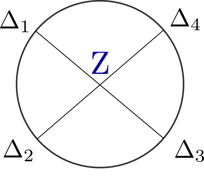
(a) A contact Witten diagram

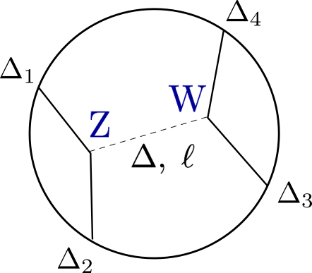
(b) An exchange Witten diagram

Figure 1: Connected four-point Witten diagrams at tree level.

While the traditional method requires the input of the precise effective Lagrangian, our position space method relies only on some qualitative features of the supergravity theory, to wit, the spectrum of supergravity fields, the selection rules encoded in the cubic vertices and a bound on the number of derivatives that can appear in the quartic vertices. The spectrum of eleven dimensional supergravity compactified on $AdS_{7}\times S^{4}$ has long been worked out in vanNieuwenhuizen:1984iz by diagonalizing the quadratic terms in the $AdS_{7}$ effective action. The spectrum is organized in infinite Kaluza-Klein towers, with increasing $USp(4)$ quantum numbers within each tower. Clearly the allowed exchanges between two pairs of half-BPS scalar KK modes are only a finite subset of the whole spectrum. There are two selection rules. The first selection rule is the R-symmetry selection rule which follows from elementary $USp(4)$ representation theory: the tensor product of two irreducible representations $[0,k]$ of $USp(4)$ yields a finite direct sum of irreps,

$$[0,k]\otimes[0,k]=\sum_{a=0}^{k}\sum_{b=0}^{a}[2(a-b),2b]\,.$$ (20)

The fields with the admissible representations have been collected in Table 1. However not all fields a priori allowed by the R-symmetry selection rule will appear in the exchange channel. Additionally, there is another selection rule, which restricts the twist $\tau$ of a field that can couple to two scalars of dimensions $\Delta_{1}$ and $\Delta_{2}$,

$$\tau<\Delta_{1}+\Delta_{2}\,.$$ (21)

In the cases of interest here, $\Delta_{1}=\Delta_{2}=2k$. The origin of this twist selection rule was discussed at length in longads5 and will not be repeated here. The spectrum and selection rules in the $AdS_{7}\times S^{4}$ supergravity background are such that truncation conditions are satisfied and all exchange diagrams are given by finite sums of $D$-functions.

field	spin	$USp(4)$ irrep	$m^{2}$	$\Delta$	$k=2$	$k=3$	$k=4$	$k=5$	$k=6$
$\varphi_{\mu\nu,k}$	2	$[0,k-2]$	$4(k-2)(k+1)$	$2k+2$	6	8	10	12	14
$A_{\mu,k}$	1	$[2,k-2]$	$4k(k-2)$	$2k+1$	5	7	9	11	13
$C_{\mu,k}$	1	$[2,k-4]$	$4(k-1)(k+1)$	$2k+3$	-	-	11	13	15
$s_{k}$	0	$[0,k]$	$4k(k-3)$	$2k$	4	6	8	10	12
$t_{k}$	0	$[0,k-4]$	$4(k-1)(k+2)$	$2k+4$	-	-	12	14	16
$r_{k}$	0	$[4,k-4]$	$4(k-2)(k+1)$	$2k+2$	-	-	10	12	14

Table 1: KK modes contributing to exchange diagrams allowed by R-symmetry selection rules.

We also make an assumption on the quartic vertices. We assume that quartic vertices with at most two spacetime derivatives effectively contribute to the four-point functions. This is necessary in order to recover the correct flat-space limit as the radius of $AdS_{7}\times S^{4}$ is sent to infinity. A further technical simplification (c.f. Appendix D of longads5 ) is that when $\Delta_{i}\neq d=6$ the contribution from the zero-derivative vertices can be absorbed, by a redefinition of parameters, into the contribution of the two-derivative vertices. This will be useful in concrete computations to avoid redundancies in the parameterization of the quartic vertices.

The position space method proceeds as follows. We use the above information on spectrum and vertices to write a general ansatz for the supergravity amplitude which consists of an exchange part and a contact part,

$$\mathcal{A}_{k}(U,V;\sigma,\tau)=\mathcal{A}_{k,{\rm exchange}}(U,V;\sigma,\tau)+\mathcal{A}_{k,{\rm contact}}(U,V;\sigma,\tau)\;.$$ (22)

Here we are working with the reduced correlator which depends only on the cross ratios and is obtained by stripping off the kinematic factor $\left(\frac{t_{12}\;t_{34}}{x_{12}^{4}x_{34}^{4}}\right)^{k}$. In this ansatz the exchange amplitude is summed over the three channels, related to one another by crossing,

$$\mathcal{A}_{k,{\rm exchange}}(U,V;\sigma,\tau)=\mathcal{A}_{k,{\rm s-ex}}(U,V;\sigma,\tau)+\mathcal{A}_{k,{\rm t-ex}}(U,V;\sigma,\tau)+\mathcal{A}_{k,{\rm u-ex}}(U,V;\sigma,\tau)\;,$$ (23)

$$\begin{split}\mathcal{A}_{k,{\rm t-ex}}(U,V;\sigma,\tau)={}&\left(\frac{U^{2}\tau}{V^{2}}\right)^{k}\mathcal{A}_{k,{\rm s-ex}}(V,U;\sigma/\tau,1/\tau)\;,\\ \mathcal{A}_{k,{\rm u-ex}}(U,V;\sigma,\tau)={}&\left(U^{2}\sigma\right)^{k}\mathcal{A}_{k,{\rm s-ex}}(1/U,V/U;1/\sigma,\tau/\sigma)\;.\end{split}$$ (24)

The s-channel exchange amplitude $\mathcal{A}_{k,{\rm s-ex}}$ is given by the sum of all s-channel exchange Witten diagrams ompatible with the selection rules for the cubic vertices. Schematically,

$$\mathcal{A}_{k,{\rm s-exchange}}=\sum_{X}\lambda_{X}Y_{R_{X}}(\sigma,\tau)\mathcal{E}_{X}(U,V)\;.$$ (25)

Here the label $X$ runs over the exchanged fields, $\mathcal{E}_{X}$ denotes the corresponding exchange Witten diagram, $Y_{R_{X}}(\sigma,\tau)$ is the polynomial associated with the irreducible representation $R_{X}$ of the field $X$ and finally $\lambda_{X}$ are the unknown coefficients to be determined. The formulae for evaluating the requisite exchange diagrams in terms contact diagrams have been given in Appendix C of longads5 , while a list of the relevant R-symmetry polynomials is given in Appendix A. For the reader’s convenience, we have also include these explicit expressions in the Mathematica notebook available from the ArXiv version of this paper.

The discussion of contribution from contact diagrams should distinguish two difference cases, as was explained in Appendix D of longads5 . When $\Delta_{i}=d$, we should include in the ansatz both the contribution from contact vertices with no derivatives and with two-derivatives. When $\Delta_{i}\neq d$, the zero-derivative contribution can be absorbed into the two-derivative contribution by redefining the parameters in the ansatz. Because of crossing symmetry, it is also convenient to split the two-derivative contribution into channels. The full contact vertex is the crossing symmetrization of the following s-channel contribution,

$$S_{\alpha_{1}\alpha_{2}\alpha_{3}\alpha_{4}}\int_{AdS_{d+1}}dX\;\frac{1}{16}(\triangledown s^{\alpha_{1}}\triangledown s^{\alpha_{2}}s^{\alpha_{3}}s^{\alpha_{4}}+s^{\alpha_{3}}s^{\alpha_{4}}\triangledown s^{\alpha_{1}}\triangledown s^{\alpha_{2}})\,,$$ (26)

where $\alpha_{i}$ collectively denote the indices of the symmetric traceless representations and $S_{\alpha_{1}\alpha_{2}\alpha_{3}\alpha_{4}}$ is an unspecified tensor symmetric under $(1\leftrightarrow 2,3\leftrightarrow 4)$. When contracted with the R-symmetry null vectors the above vertices lead to the following contribution to the s-channel contact amplitude,

$$\mathcal{A}_{k,{\rm s-cont}}\propto\sum_{0\leq a+b\leq k}c_{ab}\sigma^{a}\tau^{b}U^{2k}(\bar{D}_{2k,2k,2k,2k}-\frac{2\Gamma(2k)^{2}\Gamma(4k-2)}{\Gamma(2k+1)^{2}\Gamma(4k-3)}U\bar{D}_{2k,2k,2k+1,2k+1})\;.$$ (27)

Here we have used the so-called $\bar{D}$-functions defined by stripping off some kinematic factors from the $D$-functions,

$$\frac{\prod_{i=1}^{4}\Gamma(\Delta_{i})}{\Gamma(\Sigma-\frac{1}{2}d)}\frac{2}{\pi^{\frac{d}{2}}}D_{\Delta_{1}\Delta_{2}\Delta_{3}\Delta_{4}}(x_{1},x_{2},x_{3},x_{4})\equalscolon\frac{r_{14}^{\Sigma-\Delta_{1}-\Delta_{4}}r_{34}^{\Sigma-\Delta_{3}-\Delta_{4}}}{r_{13}^{\Sigma-\Delta_{4}}r_{24}^{\Delta_{2}}}\bar{D}_{\Delta_{1}\Delta_{2}\Delta_{3}\Delta_{4}}(U,V)\;,$$ (29)

with $\Sigma=\frac{1}{2}(\Delta_{1}+\Delta_{2}+\Delta_{3}+\Delta_{4})$. The coefficients $c_{ab}$ in (27) are symmetric thanks to the exchange symmetry $(1\leftrightarrow 2,3\leftrightarrow 4)$. When $\Delta_{i}=d$, we need to also include the zero-derivative contribution

$$\sum_{0\leq a+b\leq k}c^{\prime}_{ab}\sigma^{a}\tau^{b}U^{2k}\bar{D}_{2k,2k,2k,2k}\;,\quad\quad c^{\prime}_{ab}=c^{\prime}_{ba}\;.$$ (30)

The crossed channel contributions $\mathcal{A}_{k,{\rm t-cont}}$ and $\mathcal{A}_{k,{\rm u-cont}}$ can then be obtained from $\mathcal{A}_{k,{\rm s-cont}}$ using the crossing relation (24).

Putting all these pieces together, we now have an anstaz $\mathcal{A}_{k}(U,V;\sigma,\tau)$ of the four-point function as a finite sum of $\bar{D}$-functions. It has polynomial dependence on $\sigma$ and $\tau$ and contains linearly all the unspecified coefficients $\lambda_{X}$, $c_{ab}$, $c^{\prime}_{ab}$. These coefficients must to be fine-tuned in order to satisfy the superconformal Ward identity (8),

$$(\chi^{\prime}\partial_{\chi^{\prime}}-2\alpha^{\prime}\partial_{\alpha^{\prime}})\mathcal{G}_{k}(\chi,\chi^{\prime};\alpha,\alpha^{\prime})\big{|}_{\alpha^{\prime}\to 1/\chi^{\prime}}=0\,.$$ (31)

The ansatz $\mathcal{A}_{k}$ is not yet in a form such the superconformal Ward identity can be conveniently exploited. Fortunately, all $\bar{D}$-functions that appear in the ansatz can be reached from the basic $\bar{D}$-function $\bar{D}_{1111}$ with the repetitive use of six differential operators,

$$\begin{split}\bar{D}_{\Delta_{1}+1,\Delta_{2}+1,\Delta_{3},\Delta_{4}}={}&\mathcal{D}_{12}\bar{D}_{\Delta_{1},\Delta_{2},\Delta_{3},\Delta_{4}}:=-\partial_{U}\bar{D}_{\Delta_{1},\Delta_{2},\Delta_{3},\Delta_{4}}\;,\\ \bar{D}_{\Delta_{1},\Delta_{2},\Delta_{3}+1,\Delta_{4}+1}={}&\mathcal{D}_{34}\bar{D}_{\Delta_{1},\Delta_{2},\Delta_{3},\Delta_{4}}:=(\Delta_{3}+\Delta_{4}-\Sigma-U\partial_{U})\bar{D}_{\Delta_{1},\Delta_{2},\Delta_{3},\Delta_{4}}\;,\\ \bar{D}_{\Delta_{1},\Delta_{2}+1,\Delta_{3}+1,\Delta_{4}}={}&\mathcal{D}_{23}\bar{D}_{\Delta_{1},\Delta_{2},\Delta_{3},\Delta_{4}}:=-\partial_{V}\bar{D}_{\Delta_{1},\Delta_{2},\Delta_{3},\Delta_{4}}\;,\\ \bar{D}_{\Delta_{1}+1,\Delta_{2},\Delta_{3},\Delta_{4}+1}={}&\mathcal{D}_{14}\bar{D}_{\Delta_{1},\Delta_{2},\Delta_{3},\Delta_{4}}:=(\Delta_{1}+\Delta_{4}-\Sigma-V\partial_{V})\bar{D}_{\Delta_{1},\Delta_{2},\Delta_{3},\Delta_{4}}\;,\\ \bar{D}_{\Delta_{1},\Delta_{2}+1,\Delta_{3},\Delta_{4}+1}={}&\mathcal{D}_{24}\bar{D}_{\Delta_{1},\Delta_{2},\Delta_{3},\Delta_{4}}:=(\Delta_{2}+U\partial_{U}+V\partial_{V})\bar{D}_{\Delta_{1},\Delta_{2},\Delta_{3},\Delta_{4}}\;,\\ \bar{D}_{\Delta_{1}+1,\Delta_{2},\Delta_{3}+1,\Delta_{4}}={}&\mathcal{D}_{13}\bar{D}_{\Delta_{1},\Delta_{2},\Delta_{3},\Delta_{4}}:=(\Sigma-\Delta_{4}+U\partial_{U}+V\partial_{V})\bar{D}_{\Delta_{1},\Delta_{2},\Delta_{3},\Delta_{4}}\;.\end{split}$$ (32)

The special function $\bar{D}_{1111}$ is in fact the familiar scalar one-loop box integral in four dimensions and will be denoted as $\Phi$ from now on. It has a well-known representation in terms of dilogarithms,

$$\Phi(\chi,\chi^{\prime})=\frac{1}{\chi-\chi^{\prime}}\bigg{(}\log(\chi\chi^{\prime})\log(\frac{1-\chi}{1-\chi^{\prime}})+2{\rm Li}(\chi)-2{\rm Li}(\chi^{\prime})\bigg{)}\;,$$ (33)

and enjoys the following beautiful differential recursion relations Eden:2000bk

$$\begin{split}\partial_{\chi}\Phi={}&-\frac{1}{\chi-\chi^{\prime}}\Phi-\frac{1}{\chi(\chi-\chi^{\prime})}\ln(-1+\chi)(-1+\chi^{\prime})+\frac{1}{(-1+\chi)(\chi-\chi^{\prime})}\ln(\chi\chi^{\prime})\;,\\ \partial_{\chi^{\prime}}\Phi={}&\frac{1}{\chi-\chi^{\prime}}\Phi+\frac{1}{\chi^{\prime}(\chi-\chi^{\prime})}\ln(-1+\chi)(-1+\chi^{\prime})-\frac{1}{(-1+\chi^{\prime})(\chi-\chi^{\prime})}\ln(\chi\chi^{\prime})\;.\end{split}$$ (34)

Using the above properties of $\bar{D}$-functions, we can unambiguously decompose the supergravity ansatz into a basis spanned by $\Phi$, $\log U$, $\log V$ and 1,

$$\mathcal{A}_{k}(\chi,\chi^{\prime};\alpha,\alpha^{\prime})=R_{\Phi}\Phi(\chi,\chi^{\prime})+R_{\log U}\log U+R_{\log V}\log V+R_{1}\,,$$ (35)

where the four coefficients functions $R_{\Phi}$, $R_{\log U}$, $R_{\log V}$ and $R_{1}$ are rational functions of $\chi$, $\chi^{\prime}$ and polynomials of $\alpha$, $\alpha^{\prime}$. This decomposition makes it straightforward to enforce the superconformal Ward identity (8) on $\mathcal{A}_{k}$. Upon acting on $\mathcal{A}_{k}(\chi,\chi^{\prime};\alpha,\alpha^{\prime})$ with the differential operator $(\chi^{\prime}\partial_{\chi^{\prime}}-2\alpha^{\prime}\partial_{\alpha^{\prime}})$ from (8) and setting $\alpha^{\prime}=1/\chi^{\prime}$, a new set of coefficient functions $\widetilde{R}_{\Phi}$, $\widetilde{R}_{\log U}$, $\widetilde{R}_{\log V}$ $\widetilde{R}_{1}$ are generated from $R_{\Phi}$, $R_{\log U}$, $R_{\log V}$, $R_{1}$ with the help of the differential recursion relation of $\Phi$. The superconformal Ward identity then dictates the following conditions

$$\begin{split}{}&\widetilde{R}_{\Phi}(\chi,\chi^{\prime};\alpha,1/\chi^{\prime})=0\;,\\ {}&\widetilde{R}_{\log U}(\chi,\chi^{\prime};\alpha,1/\chi^{\prime})=0\;,\\ {}&\widetilde{R}_{\log V}(\chi,\chi^{\prime};\alpha,1/\chi^{\prime})=0\;,\\ {}&\widetilde{R}_{1}(\chi,\chi^{\prime};\alpha,1/\chi^{\prime})=0\;,\end{split}$$ (36)

which imply a large set of linear equations for the unknown coefficients. This set of equations is constraining enough to fix all relative coefficients up to an overall constant. That the overall constant should remain undetermined is inevitable because the condition (8) is homogeneous. To fix it, we demand that the OPE coefficient of the intermediate one-half BPS operator ${\cal O}^{(2)}$ has the correct value. The details of this calculation are discussed in Appendix B.

3.2 The $k=2$ four-point function

In the rest of this section we will put the above position method to work. We start with the $k=2$ one-half BPS operator $O^{(2)}$ which sits in the same short supermultiplet as the stress tensor. Its four-point function $G_{2}$ was first calculated in Arutyunov:2002ff and we will reproduce their result. By the two selection rules of cubic vertices the allowed exchanges are identified to be all the fields that belong to the $k=2$ family in Table 1. Explicitly, the exchange Witten diagrams in the s-channel contribute

$$\mathcal{A}_{2,\;{\rm s-exchange}}=Y_{11}\lambda_{s_{2}}\mathcal{E}_{s_{2}}+Y_{10}\lambda_{A_{2}}\mathcal{E}_{A_{2}}+\lambda_{\varphi_{2}}\mathcal{E}_{\varphi_{2}}\;.$$ (37)

As was discussed above, the contribution of contact Witten diagrams can be split into channels and then cross-symmetrized. Moreover, because $\Delta_{i}\neq d$ we can absorb the contribution of the zero-derivative terms into the two-derivative terms. Hence we have the following s-channel ansatz for the contact contributions,

$$\mathcal{A}_{2,\;{\rm s-contact}}=\sum_{0\leq a+b\leq 2}c_{ab}\tau^{a}\sigma^{b}\frac{\pi^{3}U^{4}}{432}(8\bar{D}_{4444}-5U\bar{D}_{5544})$$ (38)

where $c_{ab}=c_{ba}$ follows from symmetry under exchanging operators 1 and 2. The total amplitude $\mathcal{A}_{2}$ is obtained from cross-symmetrizing the above s-channel amplitude,

$$\begin{split}\mathcal{A}_{2}(U,V;\sigma,\tau)={}&\mathcal{A}_{2,s}(U,V;\sigma,\tau)+\left(\frac{U^{2}\tau}{V^{2}}\right)^{2}\mathcal{A}_{2,s}(V,U;\sigma/\tau,1/\tau)\\ {}&+\left(U^{2}\sigma\right)^{2}\mathcal{A}_{2,s}(1/U,V/U;1/\sigma,\tau/\sigma)\;,\\ \mathcal{A}_{2,s}(U,V;\sigma,\tau)={}&\mathcal{A}_{2,\;{\rm s-exchange}}(U,V;\sigma,\tau)+\mathcal{A}_{2,\;{\rm s-contact}}(U,V;\sigma,\tau)\;.\end{split}$$ (39)

Decomposing this ansatz into the basis of functions $\Phi$, $\log U$, $\log V$ and 1 and enforcing the superconformal Ward identity (36), we find enough constraints to fix all the coefficients up to an overall factor $\xi$,

$$\begin{split}{}&\lambda_{s_{2}}=\xi,\;\;\;\lambda_{A_{2}}=-\frac{1}{9}\xi,\;\;\;\lambda_{\varphi_{2}}=\frac{1}{576}\xi,\\ {}&c_{00}=\frac{1}{36}\xi,\;\;\;c_{01}=-\frac{1}{9}\xi,\;\;\;c_{02}=\frac{1}{36}\xi,\;\;\;c_{11}=-\frac{1}{12}\xi\;.\end{split}$$ (40)

The last coefficient can be determined by demanding that the relevant term in the OPE is compatible with the known value of the three-point coupling $\langle{\cal O}^{2}{\cal O}^{2}{\cal O}^{2}\rangle$. The details of this computation are relegated to Appendix B). The result is

$$\xi=\frac{15552}{\pi^{3}n^{3}}\;.$$ (41)

By setting the R-symmetry cross-ratios to the special value $\alpha=\alpha^{\prime}=1/\chi^{\prime}$ we find the following “holomorphic” correlator,

$$\mathcal{A}_{2}(\chi,\chi^{\prime};1/\chi^{\prime},1/\chi^{\prime})=\frac{2\chi^{2}((\chi-1)\chi+1)}{n^{3}(\chi-1)^{2}}\;.$$ (42)

As we show in Appendix C, it reproduces the corresponding $\mathcal{W}_{\infty}$ four-point function.

The full four-point function can also be massaged into a form consistent with the solution to the superconformal Ward identity. We found that the result can be written as

$$\mathcal{A}_{2}=\frac{\sigma\tau U^{4}}{n^{3}V^{2}}+\frac{\sigma U^{2}}{n^{3}}+\frac{\tau U^{2}}{n^{3}V^{2}}+\Upsilon\circ\left(\frac{U^{5}}{2n^{3}V}\bar{D}_{7333}\right)\;$$ (43)

where the differential operator $\Upsilon$ was defined in (12). This agrees with the result obtained by Arutynov and Sokatchev Arutyunov:2002ff . Remarkably, the inhomogeneous term ${\cal F}_{2}$ is a rational function of the cross ratios, just as in ${\cal N}=4$ super-Yang Mills, where the analogous inhomogeneous term can be identified with the free-field limit of the correlator. Of course, one could always choose the inhomogeneous term ${\cal F}$ to be rational, at the expense of making the dynamical function ${\cal H}$ more complicated. The non-trivial statement is that we can cast the correlator into a form where ${\cal F}$ is rational and ${\cal H}$ is a linear combination of $\bar{D}$-functions. This property will persist in the $k=3$ and $k=4$ examples that we study below. We conjecture that it holds in general.

3.3 The $k=3$ four-point function

We now proceed to the next Kaluza-Klein level. The allowed exchanges for $G_{3}$ include the three component fields of the $k=2$ family in Table 1 and all other fields of the $k=4$ family except for the field $t_{4}$. This field is ruled out because it has twist 12, which violates the twist upper bound. The $k=3$ family, on the other hand, is absent because of the R-symmetry selection rule. For the contact diagrams we notice that in this case the conformal dimension of the external operators coincides with the boundary spacetime dimension $\Delta=d$. As was discussed in the Appendix D of longads5 , the zero-derivative contribution can no longer be reabsorbed into the two-derivative contribution. We need to include in our ansatz both set of parameters for the quartic vertices, even if this will lead to some (harmless) ambiguities in fixing the coefficients of contact vertices when we use the superconformal Ward identity.

The s-channel ansatz is again given by an exchange part $\mathcal{A}_{3,\;{\rm s-exchange}}$ and a contact part $\mathcal{A}_{3,{\rm s-contact}}$

$$\begin{split}\mathcal{A}_{3,\;{\rm s-exchange}}=&Y_{11}\lambda_{s_{2}}\mathcal{E}_{s_{2}}+Y_{10}\lambda_{A_{2}}\mathcal{E}_{A_{2}}+Y_{00}\lambda_{\varphi_{2}}\mathcal{E}_{\varphi_{2}}\\ +&Y_{22}\lambda_{s_{4}}\mathcal{E}_{s_{4}}+Y_{21}\lambda_{A_{4}}\mathcal{E}_{A_{4}}+Y_{11}\lambda_{\varphi_{4}}\mathcal{E}_{\varphi_{4}}+Y_{20}\lambda_{r_{4}}\mathcal{E}_{r_{4}}+Y_{10}\lambda_{C_{4}}\mathcal{E}_{C_{4}}\;,\end{split}$$ (44)

$$\mathcal{A}_{3,{\rm s-contact}}=\sum_{0\leq a+b\leq 3}c_{ab}\tau^{a}\sigma^{b}\frac{7\pi^{3}U^{6}}{72000}(2\bar{D}_{6666}-U\bar{D}_{7766})+\sum_{0\leq a+b\leq 3}c^{\prime}_{ab}\tau^{a}\sigma^{b}\frac{7\pi^{3}U^{6}}{36000}\bar{D}_{6666}$$ (45)

where the coefficients $c_{ab}=c_{ba}$, $c^{\prime}_{ab}=c^{\prime}_{ba}$ are symmetric. The total amplitude ansatz is obtained by further including the t-channel and u-channel contributions which are obtained from the above s-channel contribution by crossing. Due to the ambiguity in the parameterizing of contact vertices, the superconformal Ward identity fixes only the coefficients of the exchange diagrams, leaving a subset of $c_{ab}$, $c^{\prime}_{ab}$ unfixed,

$$\begin{split}{}&\lambda_{s_{2}}=\xi,\;\;\;\lambda_{A_{2}}=-\frac{3}{50}\xi,\;\;\;\lambda_{\varphi_{2}}=\frac{1}{3600}\xi,\\ {}&\lambda_{s_{4}}=\frac{224}{135}\xi,\;\;\;\lambda_{A_{4}}=-\frac{8}{105}\xi,\;\;\;\lambda_{\varphi_{4}}=\frac{1}{5040}\xi,\;\;\;\lambda_{C_{4}}=-\frac{1}{4900}\xi,\;\;\;\lambda_{r_{4}}=\frac{16}{945}\xi,\\ {}&c_{12}=\frac{1}{140}\xi,\;\;\;c^{\prime}_{03}=\frac{1}{630}\xi,\;\;\;c^{\prime}_{11}=-\frac{17}{630}\xi,\;\;\;c^{\prime}_{12}=-\frac{13}{1260}\xi\;.\end{split}$$ (46)

These unfixed coefficients are actually redundant: the corresponding expressions are proportional to a sum of $\bar{D}$-functions which is zero in disguise, thanks to $\bar{D}$-function identities. We can then set them to zero (or to any convenient value). In Appendix B we fix the last coefficient by enforcing the correct value of the OPE coefficient of ${\cal O}^{(2)}$, which gives

$$\xi=\frac{1080000}{n^{3}\pi^{3}}\;.$$ (47)

By setting $\alpha=\alpha^{\prime}=1/\chi^{\prime}$, we extract another “holomorphic” correlator

$$\mathcal{A}_{3}(\chi,\chi^{\prime};1/\chi^{\prime},1/\chi^{\prime})=\frac{9\chi^{2}\left(2\chi^{6}-6\chi^{5}+9\chi^{4}-8\chi^{3}+9\chi^{2}-6\chi+2\right)}{4n^{3}(\chi-1)^{4}}\;,$$ (48)

which agrees with the expected result from $W_{\infty}$ (see Appendix C). As was the case for $k=2$, the $k=3$ supergravity four-point function can also be put into a compact form that manifestly solves the superconformal Ward identity,

$$\mathcal{A}_{3}=\mathcal{F}_{3,{\rm conn}}+\Upsilon\circ\mathcal{H}_{3}\;.$$ (49)

Here $\mathcal{F}_{3,{\rm conn}}$ is a simple rational function of the cross ratios,

$$\mathcal{F}_{3,{\rm conn}}=\frac{9}{4n^{3}}\left(\frac{\sigma\tau^{2}U^{6}}{V^{4}}+\frac{\sigma^{2}\tau U^{6}}{V^{2}}+\sigma^{2}U^{4}+\frac{\tau^{2}U^{4}}{V^{4}}+\sigma U^{2}+\frac{\tau U^{2}}{V^{2}}\right)\;,$$ (50)

while $\mathcal{H}_{3}$ is given in terms of $\bar{D}$-functions by the following expression,

$$\begin{split}\mathcal{H}_{3}={}&\frac{U^{5}}{48n^{3}V}\bigg{(}U^{2}(9\bar{D}_{9533}+7\bar{D}_{9544}+2\bar{D}_{9555})+\sigma(9\bar{D}_{3539}+7\bar{D}_{4549}+2\bar{D}_{5559})\\ {}&+\tau V^{2}(9\bar{D}_{3593}+7\bar{D}_{4594}+2\bar{D}_{5595})\bigg{)}\;.\end{split}$$ (51)

3.4 The $k=4$ four-point function

The calculation of the $G_{4}$ correlator is very similar to the calculation of $G_{2}$. The twist and R-symmetry selection rules dictate that the allowed exchange fields are all the component fields from the $k=2,3,4$ families in Table 1, except for $t_{6}$. This leads to the following s-channel exchange ansatz,

$$\begin{split}\mathcal{A}_{4,\;{\rm s-exchange}}=&Y_{11}\lambda_{s_{2}}\mathcal{E}_{s_{2}}+Y_{10}\lambda_{A_{2}}\mathcal{E}_{A_{2}}+Y_{00}\lambda_{\varphi_{2}}\mathcal{E}_{\varphi_{2}}\\ +&Y_{22}\lambda_{s_{4}}\mathcal{E}_{s_{4}}+Y_{21}\lambda_{A_{4}}\mathcal{E}_{A_{4}}+Y_{11}\lambda_{\varphi_{4}}\mathcal{E}_{\varphi_{4}}+Y_{20}\lambda_{r_{4}}\mathcal{E}_{r_{4}}+Y_{10}\lambda_{C_{4}}\mathcal{E}_{C_{4}}+Y_{00}\lambda_{t_{4}}\mathcal{E}_{t_{4}}\\ +&Y_{33}\lambda_{s_{6}}\mathcal{E}_{s_{6}}+Y_{32}\lambda_{A_{6}}\mathcal{E}_{A_{6}}+Y_{22}\lambda_{\varphi_{6}}\mathcal{E}_{\varphi_{6}}+Y_{31}\lambda_{r_{6}}\mathcal{E}_{r_{6}}+Y_{21}\lambda_{C_{6}}\mathcal{E}_{C_{6}}\;.\end{split}$$ (52)

Furthermore, the contribution of the zero-derivative contact vertices can be absorbed into the parameterization of the two-derivative contribution. The ansatz for the contact diagrams is thus

$$\mathcal{A}_{4,\;{\rm s-contact}}=\sum_{0\leq a+b\leq 4}c_{ab}\tau^{a}\sigma^{b}\frac{11\pi^{3}U^{8}}{474163200}(32\bar{D}_{8888}-13U\bar{D}_{9988})$$ (53)

with $c_{ab}=c_{ba}$.

Imposing the superconformal Ward identity determines all the coefficients in terms of a single parameter $\xi$,

$$\begin{split}{}&\lambda_{s_{2}}=\xi,\;\;\;\lambda_{A_{2}}=-\frac{2}{49}\xi,\;\;\;\lambda_{\varphi_{2}}=\frac{1}{12544}\xi,\\ {}&\lambda_{s_{4}}=\frac{125}{42}\xi,\;\;\;\lambda_{A_{4}}=-\frac{125}{1134}\xi,\;\;\;\lambda_{\varphi_{4}}=\frac{5}{36288}\xi,\;\;\lambda_{C_{4}}=-\frac{1}{588}\xi,\;\;\lambda_{r_{4}}=\frac{125}{756}\xi,\;\;\lambda_{t_{4}}=\frac{1}{1960}\xi,\\ {}&\lambda_{s_{6}}=\frac{33}{28}\xi,\;\;\;\lambda_{A_{4}}=-\frac{5}{154}\xi,\;\;\;\lambda_{\varphi_{4}}=\frac{5}{177408}\xi,\;\;\lambda_{C_{4}}=-\frac{25}{548856}\xi,\;\;\lambda_{r_{4}}=\frac{1}{154}\xi,\\ {}&c_{00}=-\frac{5}{1848}\xi,\;\;\;c_{01}=-\frac{5}{1386}\xi,\;\;\;c_{02}=\frac{155}{2772}\xi,\;\;\;c_{03}=-\frac{5}{1386}\xi,\;\;\;c_{04}=-\frac{5}{1848}\xi,\;\;\;\\ {}&c_{11}=\frac{1205}{5544}\xi,\;\;\;c_{12}=\frac{1235}{5544}\xi,\;\;\;c_{13}=-\frac{5}{2772}\xi,\;\;\;c_{22}=\frac{25}{396}\xi\,.\end{split}$$ (54)

Finally, $\xi$ is fixed by comparing with the OPE coefficient of the intermediate ${\cal O}^{(2)}$ operator (see Appendix B),

$$\xi=\frac{16595712}{n^{3}\pi^{3}}\;.$$ (55)

The “holomorphic” correlator is given by

$$\mathcal{A}_{4}(\chi,\chi^{\prime};1/\chi^{\prime},1/\chi^{\prime})=\frac{8\chi^{2}\left(\chi^{2}-\chi+1\right)^{2}\left(5\chi^{6}-15\chi^{5}+9\chi^{4}+7\chi^{3}+9\chi^{2}-15\chi+5\right)}{5n^{3}(\chi-1)^{6}}\;,$$ (56)

which is again in agreement with the $W_{\infty}$ result, see Appendix C. Finally, we recast the result in a way that makes superconformal symmetry manifest,

$$\mathcal{A}_{4}=\mathcal{F}_{4,{\rm conn}}+\Upsilon\circ\mathcal{H}_{4}\;.$$ (57)

Here, the “inhomogenous” term $\mathcal{F}_{4,{\rm conn}}$ is the following rational function of the cross ratios,

$$\begin{split}\mathcal{F}_{4,{\rm conn}}={}&\frac{4U^{2}\left(\sigma\tau^{3}U^{6}+\sigma^{3}\tau U^{6}V^{4}+\tau^{3}U^{4}+\sigma^{3}U^{4}V^{6}+\sigma V^{6}+\tau V^{4}\right)}{n^{3}V^{6}}\\ {}&+\frac{718U^{4}\left(\tau^{2}+\sigma^{2}\tau^{2}U^{4}+\sigma^{2}V^{4}\right)}{275n^{3}V^{4}}-\frac{776\sigma\tau U^{4}\left(\tau U^{2}+\sigma U^{2}V^{2}+V^{2}\right)}{275n^{3}V^{4}}\;,\end{split}$$ (58)

while the dynamical function $\mathcal{H}_{4}$ is a linear combination of $\bar{D}$-functions. It is most conveniently represented as a sum over three channels,

$$\mathcal{H}_{4}=\mathcal{H}_{4s}+\mathcal{H}_{4t}+\mathcal{H}_{4u}\;.$$ (59)

The s-channel is given by

$$\begin{split}\mathcal{H}_{4s}={}&\frac{U^{9}}{475200n^{3}V}\bigg{(}7920\bar{D}_{11,7,3,3}+8496\bar{D}_{11,7,4,4}+4040\bar{D}_{11,7,5,5}\\ {}&+1100\bar{D}_{11,7,6,6}+165\bar{D}_{11,7,7,7}\bigg{)}+\frac{\tau U^{9}}{118800n^{3}V^{3}}\bigg{(}4308\bar{D}_{11,5,3,5}\\ {}&+825V^{2}\bar{D}_{11,7,5,5}+605V^{2}\bar{D}_{11,7,6,6}+165V^{2}\bar{D}_{11,7,7,7}+3088V\bar{D}_{11,6,4,5}\\ {}&+2240V\bar{D}_{11,6,5,6}+605V\bar{D}_{11,6,6,7}+3088\bar{D}_{11,5,4,6}+825\bar{D}_{11,5,5,7}\bigg{)}\,,\end{split}$$ (60)

and the t- and u-channels are obtained by the substitution rules

$$\begin{split}\mathcal{H}_{4t}={}&\mathcal{H}_{4s}(U\to U/V,V\to 1/V;\sigma\to\tau,\tau\to\sigma)\;,\\ \mathcal{H}_{4u}={}&U^{8}\sigma^{2}\mathcal{H}_{4s}(U\to 1/U,V\to V/U;\sigma\to 1/\sigma,\tau\to\tau/\sigma)\;.\end{split}$$ (61)

4 Mellin space

The position space method discussed in the previous section is a rigorous algorithm to compute four-point functions without a priori knowing the vertices. Though much easier than the traditional approach, this method also runs out of steam as one moves up in the Kaluza-Klein towers due to unmanageable computational complexity and does not appear promising to provide a general solution. What’s more, the position space method presents the final answer as an unintuitive sum of contact Witten diagrams. The most suitable language to address both problems is the Mellin representation initiated by Mack Mack:2009mi and developed by Penedones and others Penedones:2010ue ; Paulos:2011ie ; Fitzpatrick:2011ia ; Costa:2012cb ; Fitzpatrick:2012cg ; Costa:2014kfa ; Goncalves:2014rfa . We refer the reader to longads5 for a detailed review of this formalism. We will be very brief here.

Using the inverse Mellin transformation, we express the connected part of the four-point function as a double integral

$$\begin{split}G_{k,{\rm conn}}={}&\sum_{L+M+N=k}a^{L}b^{M}c^{N}\int_{-i\infty}^{i\infty}\frac{ds}{2}\;\frac{dt}{2}\;A^{s/2-2k}B^{u/2-2k}C^{t/2-2k}\\ {}&\times\mathcal{M}_{k,\;LMN}(s,t)\Gamma^{2}[-\frac{s}{2}+2k]\Gamma^{2}[-\frac{t}{2}+2k]\Gamma^{2}[-\frac{u}{2}+2k]\;.\end{split}$$ (62)

For notational convenience we have introduced

$$\begin{split}A\colonequals{}&x^{2}_{12}x^{2}_{34}\;,\;\;\;\;B\colonequals x^{2}_{13}x^{2}_{24}\;,\;\;\;\;C\colonequals x^{2}_{14}x^{2}_{23}\;,\\ a\colonequals{}&t_{12}t_{34}\;,\;\;\;\;b\colonequals t_{13}t_{24}\;,\;\;\;\;c\colonequals t_{14}t_{23}\;.\\ \end{split}$$ (63)

The variables $s$, $t$ and $u$ are interpreted as “Mandelstam variables” and satisfy the constraint $s+t+u=8k$. The integration of the two independent variables $s$, $t$ is performed along the imaginary axis. We further define the Mellin amplitude $\mathcal{M}(s,t;\sigma,\tau)$ a sum of the partial amplitudes from $\mathcal{M}_{k,\;LMN}$,

$$\mathcal{M}(s,t;\sigma,\tau)=a^{-k}\sum_{L+M+N=k}a^{L}b^{M}c^{N}\mathcal{M}_{k,\;LMN}(s,t)\;.$$ (64)

The above representation (62) of the crossing invariant correlator $G_{k,{\rm conn}}$ makes the following symmetry properties of the partial amplitudes clear,

$$\begin{split}\mathcal{M}_{k,\;NML}(t,s)={}&\mathcal{M}_{k,\;LMN}(s,t)\;,\\ \mathcal{M}_{k,\;MNL}(u,t)={}&\mathcal{M}_{k,\;LMN}(s,t)\;,\end{split}$$ (65)

which in turn imply simple crossing symmetry relations for the Mellin amplitude $\mathcal{M}$,

$$\begin{split}\sigma^{k}{\mathcal{M}}_{k}(u,t;1/\sigma,\tau/\sigma)={}&{\mathcal{M}}_{k}(s,t,;\sigma,\tau)\;,\\ \tau^{k}{\mathcal{M}}_{k}(t,s;\sigma/\tau,1/\tau)={}&{\mathcal{M}}_{k}(s,t;\sigma,\tau)\;.\end{split}$$ (66)

The Mellin amplitude bears several formal similarities with the flat space S-matrix. Being analogous to amputated on-shell tree-level Feynman diagrams in flat space, tree-level Witten diagrams admit extremely simple representations in Mellin space. If we temporarily suppress the dependence on R-symmetry variables, then (62) reduces to

$$G_{k,{\rm conn}}=\int_{-i\infty}^{i\infty}\frac{ds}{2}\;\frac{dt}{2}\;A^{s/2-2k}B^{u/2-2k}C^{t/2-2k}\mathcal{M}(s,t)\Gamma^{2}[-\frac{s}{2}+2k]\Gamma^{2}[-\frac{t}{2}+2k]\Gamma^{2}[-\frac{u}{2}+2k]\;.$$ (67)

The contact Witten diagram with a nonderivative vertex is just a constant in Mellin space. More generally, the contact Witten diagram with a $2n$-derivatives vertex yields a polynomial of degree $n$ in the Mandelstam variables Penedones:2010ue . Exchange diagrams also have a simple structure in Mellin space, as a sum over simple poles with polynomial residues plus another regular polynomial piece Costa:2012cb ,

$$\mathcal{M}_{\rm exchange}(s,t)=\sum_{m=0}^{\infty}\frac{Q_{J,m}(t)}{s-\tau-2m}+P_{J-1}(s,t)$$ (68)

Here we have considered an s-channel exchange Witten diagram with an exchanged field of conformal dimension $\Delta$ and spin $J$ (and hence twist $\tau=\Delta-J$). The functions $Q_{J,m}(t)$ and $P_{J-1}(s,t)$ are polynomials of degrees $J$ and $J-1$, respectively. When the twist of the exchanged field satisfies the condition

$$\tau=4k-2m\;,\quad\quad m\in\mathbb{Z}_{\geqslant 0}$$ (69)

a remarkable simplification occurs: the infinite sum in (68) truncates to finitely many terms (see Section 3.2 of longads5 for a detailed discussion). This is the Mellin-space counterpart of the fact that certain exchange Witten diagrams can be evaluated as finitely many contact Witten diagrams. The spectrum condition (69) is precisely met by the eleven dimensional supergravity on $AdS_{7}\times S^{4}$. For this reason the analytic structure of the Mellin amplitude of the $AdS_{7}\times S^{4}$ four-point function is extremely simple: it has just finitely many simple poles and some extra polynomial terms.

4.1 Superconformal symmetry in Mellin space

In position space, superconformal symmetry of the four-point function is encoded in the solution of the superconformal Ward identity,

$${\cal G}_{k,{\rm conn}}={\cal F}_{k,{\rm conn}}+\Upsilon\circ{\cal H}_{k,{\rm conn}}\,.$$ (70)

Our position space results have led us to conjecture that in the supergravity limit we can take ${\cal H}_{k}$ to be a linear combination of $\bar{D}$-functions, and $\mathcal{F}_{k,{\rm conn}}$ to be rational function of the cross ratios. The details of this section are very technical, but the main result is easy to summarize. We are going to find that Mellin version of (70) takes the form

$$\mathcal{M}_{k}=\widehat{\Theta}\circ\widetilde{\mathcal{M}}_{k}\;,$$ (71)

where $\widetilde{\mathcal{M}}_{k}$ is an “auxiliary” Mellin amplitude defined from the dynamical function ${\cal H}_{k,{\rm conn}}$, see (73), and $\widehat{\Theta}$ a somewhat complicated difference operator defined in (83).

We start by writing the Mellin transformation of the left-hand side of (70) using (62),

$$\mathcal{G}_{k,{\rm conn}}=\int_{-i\infty}^{i\infty}\frac{ds}{2}\frac{dt}{2}U^{\frac{s}{2}}V^{\frac{t}{2}-2k}\mathcal{M}_{k}(s,t;\sigma,\tau)\Gamma^{2}[-\frac{s}{2}+2k]\Gamma^{2}[-\frac{t}{2}+2k]\Gamma^{2}[-\frac{u}{2}+2k]\;.$$ (72)

Consider now the right-hand side of (70). The Mellin transform of the rational function $\mathcal{F}_{k,{\rm conn}}$ is ill-defined. As explained in longads5 , it can be defined as “zero”. On the other hand, we can write a Mellin representation for the dynamical function $\mathcal{H}_{k}$ in terms of an “auxiliary” Mellin amplitude $\widetilde{\mathcal{M}}_{k}(s,t;\sigma,\tau)$

$$\mathcal{H}_{k}=\int_{-i\infty}^{i\infty}\frac{ds}{2}\frac{dt}{2}U^{\frac{s}{2}+1}V^{\frac{t}{2}-2k+1}\widetilde{\mathcal{M}}_{k}(s,t;\sigma,\tau)\Gamma^{2}[-\frac{s}{2}+2k]\Gamma^{2}[-\frac{t}{2}+2k]\Gamma^{2}[-\frac{\tilde{u}}{2}+2k]$$ (73)

where $\tilde{u}=u-6$. As we demonstrate the shift has the virtue of giving simple transformation properties to $\widetilde{\mathcal{M}}_{k}(s,t;\sigma,\tau)$ under crossing,

$$\begin{split}\sigma^{k-2}{\widetilde{\mathcal{M}}}_{k}(\tilde{u},t;1/\sigma,\tau/\sigma)={}&{\widetilde{\mathcal{M}}}_{k}(s,t,;\sigma,\tau)\;,\\ \tau^{k-2}{\widetilde{\mathcal{M}}}_{k}(t,s;\sigma/\tau,1/\tau)={}&{\widetilde{\mathcal{M}}}_{k}(s,t;\sigma,\tau)\;.\end{split}$$

In the auxiliary amplitude $\widetilde{\mathcal{M}}_{k}(s,t;\sigma,\tau)$, the triplet variables $(s,t,\tilde{u})$ replaces $(s,t,u)$ to become the set of variables that permute under crossing. This becomes especially evident after we restore all the factors of $x_{ij}^{2}$ and $t_{ij}$. Restoring this factor will also facilitate the extraction of the difference operator. Let us see this in detail.

We first note that the combination

$$a^{k}A^{-2k}\Upsilon\circ\mathcal{H}_{k}$$ (74)

is crossing invariant, since it has the same crossing properties as $G_{k}$. Upon inserting the inverse Mellin transformation (73) into (74) and decomposing the auxiliary amplitude with respect to the R-symmetry monomials,

$$\widetilde{\mathcal{M}}(s,t;\sigma,\tau)=\sum_{l+m+n=k-2}\sigma^{m}\tau^{n}\;\widetilde{\mathcal{M}}_{k,\;lmn}(s,t)\;,$$ (75)

we find

$$(\frac{a}{A^{2}})^{k}\;\Upsilon\circ\sum_{l+m+n=k-2}\int_{-i\infty}^{i\infty}\frac{ds}{2}\;\frac{dt}{2}\;U^{s/2+1}V^{t/2-2k+1}\sigma^{m}\tau^{n}\widetilde{\mathcal{M}}_{k,\;lmn}(s,t)\;\tilde{\Gamma}_{3}(s,t)\;.$$ (76)

Here the factor $\tilde{\Gamma}_{3}(s,t)$ is short-hand for $\Gamma^{2}[-\frac{s}{2}+2k]\Gamma^{2}[-\frac{t}{2}+2k]\Gamma^{2}[-\frac{\tilde{u}}{2}+2k]$. We now let the differential operator $\Upsilon$ act on the monomial $U^{s/2+1}V^{t/2-2k+1}\sigma^{m}\tau^{n}$, leading to the following integral

$$\int_{-i\infty}^{i\infty}\frac{ds}{2}\;\frac{dt}{2}\;\sum_{l+m+n=k-2}a^{l}b^{m}c^{n}A^{s/2-2k}B^{\tilde{u}/2-2k}C^{t/2-2k}\;\Theta\;\widetilde{\mathcal{M}}_{k,\;lmn}(s,t)\;\tilde{\Gamma}_{3}(s,t)\;,$$ (77)

where $U=A/B$, $V=C/B$, $\sigma=b/a$, $\tau=c/a$ have been substituted back into the expression. The factor $\Theta$ is a polynomial of $A$, $B$, $C$, $a$, $b$, $c$ and $s$, $t$ obtained from the action of the differential operator $\Upsilon$ on the monomial $U^{s/2+1}V^{t/2-2k+1}\sigma^{m}\tau^{n}$. To write an explicit expression for $\Theta$, it is useful further to introduce the following combinations of Mandelstam variables,

$$\begin{split}X={}&s+4l-4k+2\;,\\ Y={}&t+4n-4k+2\;,\\ \tilde{Z}={}&\tilde{u}+4m-4k+2\;.\end{split}$$ (78)

In terms of these variables, $\Theta$ reads

$$\begin{split}\Theta={}&-\frac{1}{4}\bigg{[}abC^{3}X\tilde{Z}+aB^{3}cXY+A^{3}bcY\tilde{Z}\\ +{}&A^{2}bC(c(X+4)\tilde{Z}-(Y+2)\tilde{Z}(a-b+c))+AbC^{2}(a(Y+4)\tilde{Z}-(X+2)\tilde{Z}(a-b+c))\\ +{}&aBC^{2}(X(\tilde{Z}+2)(a-b-c)+bX(Y+4))+A^{2}Bc(b(4+X)Y-(a+b-c)Y(2+\tilde{Z}))\\ +{}&aB^{2}C((a-b-c)X(2+Y)+cX(4+\tilde{Z}))\\ +{}&AB^{2}c((-a-b+c)(2+X)Y+aY(4+\tilde{Z}))\\ +{}&ABC\big{(}a^{2}(Y+2)(\tilde{Z}+2)+b^{2}(X+2)(Y+2)+c^{2}(X+2)(\tilde{Z}+2)\\ {}&+bc(2+X)(4+X)+ab(2+Y)(4+Y)+ac(2+\tilde{Z})(4+\tilde{Z})\big{)}\bigg{]}\;.\end{split}$$ (79)

The reader should not focus on this complicated expression because further manipulations will soon lead to a major simplification. At this stage we only want to point out that the above expression of $\Theta$ can be checked to be crossing invariant under any permutation of the triplets

$$(a,A,s)\;,\quad\quad(b,B,\tilde{u})\;,\quad\quad(c,C,t)\;.$$ (80)

Crossing invariance of (77) implies the following crossing identities for $\widetilde{\mathcal{M}}_{k,\;lmn}(s,t)$,

$$\begin{split}\widetilde{\mathcal{M}}_{k,\;nml}(t,s)={}&\widetilde{\mathcal{M}}_{k,\;lmn}(s,t)\;,\\ \widetilde{\mathcal{M}}_{k,\;mnl}(\tilde{u},t)={}&\widetilde{\mathcal{M}}_{k,\;lmn}(s,t)\;,\end{split}$$ (81)

from which the crossing identities (4.1) of $\widetilde{\mathcal{M}}_{k}(s,t;\sigma,\tau)$ immediately follow.

As in Rastelli:2016nze ; longads5 , we should reinterpret the monomials of $A$, $B$, $C$ in (79) as difference operators acting on functions of $s$, $t$ in the integrand, thus promoting the factor $\Theta$ to an operator $\widehat{\Theta}$. This operator $\widehat{\Theta}$ can be written in a compact form if the respective shift on $X$, $Y$ and $\tilde{Z}$ has first been performed, as we now show. All monomials that appear in $\Theta$ have the form $A^{\alpha}B^{3-\alpha-\beta}C^{\beta}$. Multiplying an inverse Mellin integral by such a monomial, we have

$$A^{\alpha}B^{3-\alpha-\beta}C^{\beta}\int_{\cal C}{ds}{dt}\,A^{s/2-2k}B^{\tilde{u}/2-2k}C^{t/2-2k}F(s,t)=$$ (82)

$$\int_{\cal C^{\prime}}dsdtA^{s/2-2k}B^{u/2-2k}C^{t/2-2k}F(s-2\alpha,t-2\beta)\;.$$

(The shift of the integration contour is important in producing rational terms by the mechanism discussed in longads5 . Here we are focusing on the Mellin amplitude and ignore contour issues.) Note that in the first term we use the shifted Mandelstam variable $\tilde{u}=u-6=8k-s-t-6$, while the unshifted $u$ appears in the second term. We conclude that multiplication by the monomial $A^{\alpha}B^{3-\alpha-\beta}C^{\beta}$ corresponds in Mellin space to a difference operator that shifts $s\to s-2\alpha$ and $t\to t-2\beta$.

Interpreting every monomials in $\Theta$ in this fashion we find a difference operator $\widehat{\Theta}$. We can make the expression of $\widehat{\Theta}$ very compact by performing the shift in two stages: first we shift on the factor of $X$, $Y$, $\tilde{Z}$ multiplying each monomial $A^{\alpha}B^{3-\alpha-\beta}C^{\beta}$ and bring it the left; then $A^{\alpha}B^{3-\alpha-\beta}C^{\beta}$ remains an operator to act on whatever is in the integrand on the right. We arrive at the following simple expression,

$$\widehat{\Theta}=-\frac{1}{4}\big{(}(XY)\widehat{B\mathfrak{R}}+(XZ)\widehat{C\mathfrak{R}}+(YZ)\widehat{A\mathfrak{R}}\big{)}$$ (83)

where we defined an “unshifted” $Z$ variable

$$Z\colonequals\tilde{Z}+6=u+4m-4k+2\;$$ (84)

and the crossing-invariant factor $\mathfrak{R}$ is given by

$$\mathfrak{R}=a^{2}BC+b^{2}AC+c^{2}AB+abC(-A-B+C)+acB(-A+B-C)+bcA(A-B-C)$$ (86)

The expressions $\widehat{A\mathfrak{R}}$, $\widehat{B\mathfrak{R}}$, $\widehat{C\mathfrak{R}}$ are written shorthands that should be understood as follows: one first expands $A\mathfrak{R}$, $B\mathfrak{R}$, $C\mathfrak{R}$ into monomials $A^{\alpha}B^{3-\alpha-\beta}C^{\beta}$ and then regards each of them as the operator $\widehat{A^{\alpha}B^{3-\alpha-\beta}C^{\beta}}$. These operators will only act on objects multiplied from the right and will no longer shift the $X$, $Y$, $Z$ factors multiplied from the left.

We can now give the explicit action of $\widehat{A^{\alpha}B^{3-\alpha-\beta}C^{\beta}}$ as an operator that transforms a term of $\widetilde{\mathcal{M}}_{k}$ into a term of $\mathcal{M}_{k}$,

$$\begin{split}\widehat{A^{\alpha}B^{3-\alpha-\beta}C^{\beta}}{}&\circ\widetilde{\mathcal{M}}_{k,\;lmn}(s,t)\colon=\widetilde{\mathcal{M}}_{k,\;lmn}(s-2\alpha,t-2\beta)\\ \times{}&\frac{\Gamma^{2}[-\frac{s}{2}+2k+\alpha]\Gamma^{2}[-\frac{t}{2}+2k+\beta]\Gamma^{2}[-\frac{u}{2}+2k+(3-\alpha-\beta)]}{\Gamma^{2}[-\frac{s}{2}+2k]\Gamma^{2}[-\frac{t}{2}+2k]\Gamma^{2}[-\frac{u}{2}+2k]}\;.\end{split}$$ (87)

This action is obtained by applying the aforementioned shift of $s$ and $t$ on the integrand and taking into consideration the difference of Gamma function factors between the definitions (62) and (77).

To summarize, the superconformal Ward identity implies that the full Mellin amplitude $\mathcal{M}_{k}$ can be written in terms of an auxiliary amplitude $\widetilde{\mathcal{M}}_{k}$ acted upon by the difference operator $\widehat{\Theta}$,

$$\mathcal{M}_{k}=\widehat{\Theta}\circ\widetilde{\mathcal{M}}_{k}\;.$$ (88)

The operator $\widehat{\Theta}$ is given by (83) where each monomial operator acts as in (87).

4.2 Consistency conditions and the algebraic problem

We now take stock and summarize the conditions on the Mellin amplitude that follow from our discussion in the previous sections:

1. Crossing symmetry: As the external operators are identical bosonic operators, the Mellin amplitude ${\mathcal{M}}_{k}$ satisfies the crossing relations

   $$\begin{split}\sigma^{k}{\mathcal{M}}_{k}(u,t;1/\sigma,\tau/\sigma)={}&{\mathcal{M}}_{k}(s,t,;\sigma,\tau)\\ \tau^{k}{\mathcal{M}}_{k}(t,s;\sigma/\tau,1/\tau)={}&{\mathcal{M}}_{k}(s,t;\sigma,\tau)\,.\end{split}$$ (89)

2. Analytic properties: $\mathcal{M}_{k}$ has only simple poles in correspondence with the exchanged single-trace operators. Denoting the position of the simple poles in the s-, t- and u-channel as $s_{0}$, $t_{0}$, $u_{0}$, they are:

   $$\begin{split}s_{0}={}&4,6,\ldots,4k-2\;,\\ t_{0}={}&4,6,\ldots,4k-2\;,\\ u_{0}={}&4,6,\ldots,4k-2\;.\end{split}$$ (90)

   Moreover, the residue at any of the poles must be a polynomial in the other Mandelstam variable.

3. Asymptotic behavior: $\mathcal{M}_{k}$ should grow at most linearly in the asymptotic regime of large Mandelstam variables,

   $$\mathcal{M}_{k}(\beta s,\beta t,\beta u,\sigma,\tau)\sim O(\beta)\;,\quad\quad\quad\beta\to\infty\;.$$ (91)

4. Superconformal symmetry: $\mathcal{M}_{k}$ can be written in terms an auxiliary amplitude $\widetilde{\mathcal{M}}_{k}$ acted upon by the difference operator $\widehat{\Theta}$,

   $$\mathcal{M}_{k}=\widehat{\Theta}\circ\widetilde{\mathcal{M}}_{k}\;,$$ (92)

   where the action of $\widehat{\Theta}$ has been defined in the previous subsection.

The name of the game is to find a function $\widetilde{\mathcal{M}}_{k}(s,t;\sigma,\tau)$ such that all the conditions are simultaneously satisfied. We leave a detailed analysis of this very constrainted “bootstrap” problem for the future. As in the four-dimensional case analyzed in Rastelli:2016nze ; longads5 , we find it very plausible that this problem has a unique solution (up to overall rescaling).

4.3 Solutions from the position space method

In this subsection we give solutions to the algebraic problem defined above for $k=2,3,4$. These solutions are obtained from the position space results, but look much simpler in Mellin space when the prescription (92) is implemented.

$k=2$

We start from the simplest example of $k=2$. In this case, the homogenous part $\mathcal{H}_{2}$ is a degree-0 polynomial of $\sigma$ and $\tau$. Therefore there is only one R-symmetry structure in the auxiliary amplitude $\widetilde{\mathcal{M}}_{2}$. The answer is given by

$$\widetilde{\mathcal{M}}_{2}(s,t;\sigma,\tau)=\frac{32}{n^{3}(s-6)(s-4)(t-6)(t-4)(\tilde{u}-6)(\tilde{u}-4)}\;$$ (93)

which is manifestly symmetric under the permutation of $s$, $t$ and $\tilde{u}$.

$k=3$

Moving on to the next simplest case of $k=3$, we know that $\mathcal{H}_{3}$ is a degree-one polynomial of $\sigma$ and $\tau$ and therefore consists of three terms. The three R-symmetry monomials $\sigma$, $\tau$, $1$ are in the same orbit under the action of the crossing symmetry group. Hence, $\widetilde{\mathcal{M}}_{3,010}$ and $\widetilde{\mathcal{M}}_{3,001}$ are related to $\widetilde{\mathcal{M}}_{3,100}$ via (81)

$$\widetilde{\mathcal{M}}_{3,010}(s,t)=\widetilde{\mathcal{M}}_{3,100}(\tilde{u},t),\;\;\;\;\;\;\;\;\;\;\widetilde{\mathcal{M}}_{3,001}(s,t)=\widetilde{\mathcal{M}}_{3,100}(t,s).$$ (94)

Finally, $\widetilde{\mathcal{M}}_{3,100}$ is given by

$$\widetilde{\mathcal{M}}_{3,100}(s,t)=\frac{8(s-7)}{3n^{3}(s-8)(s-6)(s-4)(t-10)(t-8)(\tilde{u}-10)(\tilde{u}-8)}\;,$$ (95)

and the full auxiliary Mellin amplitude is

$$a\widetilde{\mathcal{M}}_{3}(s,t;\sigma,\tau)=a\widetilde{\mathcal{M}}_{3,100}(s,t)+b\widetilde{\mathcal{M}}_{3,010}(s,t)+c\widetilde{\mathcal{M}}_{3,001}(s,t)\;.$$ (96)

$k=4$

$\mathcal{H}_{4}$ is a degree-2 polynomial of $\sigma$ and $\tau$ and therefore the auxiliary amplitude contains six R-symmetry monomials. Crossing symmetry groups these six terms into two orbits $(1,\sigma^{2},\tau^{2})$ and $(\sigma,\tau,\sigma\tau)$, within in each amplitudes are related by (81),

$$\begin{split}\widetilde{\mathcal{M}}_{4,200}(s,t)={}&\widetilde{\mathcal{M}}_{4,020}(\tilde{u},t)=\widetilde{\mathcal{M}}_{4,002}(t,s)\;,\\ \widetilde{\mathcal{M}}_{4,011}(s,t)={}&\widetilde{\mathcal{M}}_{4,101}(\tilde{u},t)=\widetilde{\mathcal{M}}_{4,110}(t,s)\;.\end{split}$$ (97)

The two independent auxiliary amplitudes turn out to be

$$\begin{split}\widetilde{\mathcal{M}}_{4,200}(s,t)={}&\frac{1}{7425n^{3}}\prod_{i=2}^{7}\frac{1}{s-2i}\prod_{j=6}^{7}\frac{1}{t-2j}\prod_{k=6}^{7}\frac{1}{\tilde{u}-2k}\\ \times{}&\left(165s^{4}-6820s^{3}+102620s^{2}-661648s+1525632\right)\;,\\ \widetilde{\mathcal{M}}_{4,101}(s,t)={}&\frac{4}{7425n^{3}}\prod_{i=4}^{7}\frac{1}{s-2i}\prod_{j=4}^{7}\frac{1}{t-2j}\prod_{k=6}^{7}\frac{1}{\tilde{u}-2k}\\ \times{}&(165s^{2}t^{2}-4180s^{2}t+26180s^{2}-4180st^{2}+105980st\\ {}&-664424s+26180t^{2}-664424t+4170432)\;\end{split}$$ (98)

and the full auxiliary amplitude is

$$\begin{split}a^{2}\widetilde{\mathcal{M}}_{4}(s,t;\sigma,\tau)={}&a^{2}\widetilde{\mathcal{M}}_{4,200}(s,t)+b^{2}\widetilde{\mathcal{M}}_{4,020}(s,t)+c^{2}\widetilde{\mathcal{M}}_{4,002}(s,t)\\ +{}&ab\widetilde{\mathcal{M}}_{4,110}(s,t)+bc\widetilde{\mathcal{M}}_{4,011}(s,t)+ac\widetilde{\mathcal{M}}_{4,101}(s,t)\end{split}$$ (99)

The above expression is much more complicated than those for $k=2$ and $k=3$, but the auxiliary amplitude is still significantly simpler than the full amplitude. We have not yet been able to discern a pattern that would allow to guess the auxiliary amplitude for general $k$.

Aknowledgement

We thank Eric Perlmutter for helpful discussions on the $\mathcal{W}_{n}$ four-point functions. Our work is supported in part by NSF Grant PHY-1620628.

Appendix A R-symmetry polynomials

We collect here the R-symmetry polynomials Nirschl:2004pa needed for the position space method:

$$\begin{split}Y_{00}=&1\;,\\ Y_{10}=&\sigma-\tau\;,\\ Y_{11}=&\sigma-\tau-\frac{2}{d}\;,\\ Y_{20}=&\sigma^{2}+\tau^{2}-2\sigma\tau-\frac{2}{d-2}(\sigma+\tau)+\frac{2}{(d-2)(d-1)}\;,\\ Y_{21}=&\sigma^{2}-\tau^{2}-\frac{4}{d+2}(\sigma-\tau)\;,\\ Y_{22}=&\sigma^{2}+\tau^{2}+4\sigma\tau-\frac{8}{d+4}(\sigma+\tau)+\frac{8}{(d+2)(d+4)}\;,\\ Y_{30}=&\sigma^{3}-3\sigma^{2}\tau+3\sigma\tau^{2}-\tau^{3}-\frac{6}{d}(\sigma^{2}-\tau^{2})+\frac{12}{d(d+1)}(\sigma-\tau)\;,\\ Y_{31}=&\sigma^{3}-\sigma^{2}\tau-\sigma\tau^{2}+\tau^{3}-\frac{8(d-1)}{(d+4)(d-2)}(\sigma^{2}+\tau^{2})+\frac{8(d-6)}{(d+4)(d-2)}\sigma\tau\\ {}&+\frac{4(3d+2)}{(d+1)(d+4)(d-2)}(\sigma+\tau)-\frac{8}{(d+1)(d+4)(d-2)}\;,\\ Y_{32}=&\sigma^{3}+3\sigma^{2}\tau-3\sigma\tau^{2}-\tau^{3}-\frac{12}{d+6}(\sigma^{2}-\tau^{2})+\frac{24}{(d+4)(d+6)}(\sigma-\tau)\;,\\ Y_{33}=&\sigma^{3}+9\sigma^{2}\tau+9\sigma\tau^{2}+\tau^{3}-\frac{18}{d+8}(\sigma^{2}+\tau^{2})-\frac{72}{d+8}\sigma\tau\\ {}&+\frac{72}{(d+6)(d+8)}(\sigma+\tau)-\frac{48}{(d+4)(d+6)(d+8)}\;.\\ \end{split}$$ (100)

In the above expressions $d\equiv 5$. The $USp(4)$ Dynkin labels $[2(a-b),2b]$ are related to the labels $(m,n)$ in $Y_{nm}$ via $n=a$, $m=b$.

Appendix B Fixing the overall constant

In Section 3 we have shown in examples how the superconformal Ward identity determines all the coefficients of the position space ansatz, up to an overall scaling factor $\xi$. To fix the overall normalization, we are going to demand that the singular terms of the four-point function that correspond to exchanged one-half BPS operators in (say) the s-channel OPE have the correct coefficients. Those coefficients are read off from the one-half BPS three-point functions, which have been computed both in supergravity Corrado:1999pi ; Bastianelli:1999en and using the $W_{\infty}$ algebra Beem:2014kka ,

$$\begin{split}{}&\langle{\cal O}^{(k_{1})}_{\alpha_{1}}(x_{1}){\cal O}^{(k_{2})}_{\alpha_{2}}(x_{2}){\cal O}^{(k_{3})}_{\alpha_{3}}(x_{3})\rangle=\frac{C(k_{1},k_{2},k_{3})}{x_{12}^{2k_{123}}x_{23}^{2k_{231}}x_{31}^{2k_{312}}}\langle C^{\alpha_{1}}C^{\alpha_{2}}C^{\alpha_{3}}\rangle\;,\\ {}&C(k_{1},k_{2},k_{3})=\frac{2^{2\beta-2}}{(\pi n)^{\frac{3}{2}}}\Gamma\bigg{(}\frac{k_{1}+k_{2}+k_{3}}{2}\bigg{)}\frac{\Gamma(\frac{k_{123}+1}{2})\Gamma(\frac{k_{231}+1}{2})\Gamma(\frac{k_{312}+1}{2})}{\sqrt{\Gamma(2k_{1}-1)\Gamma(2k_{2}-1)\Gamma(2k_{3}-1)}}\;,\\ {}&k_{ijk}\colon=k_{i}+k_{j}-k_{k}\;,\\ {}&\beta=\frac{k_{1}+k_{2}+k_{3}}{2}\;,\end{split}$$ (101)

where unit normalized two-point functions are assumed. Here $C_{\alpha_{i}}^{I_{1}\ldots I_{k_{i}}}$ form a basis of symmetric traceless tensors of the R-symmetry group and we labeled such representations with $\alpha_{i}$. The factor $\langle C_{\alpha_{1}}C_{\alpha_{2}}C_{\alpha_{3}}\rangle$ is the unique scalar contraction of $C_{\alpha_{i}}^{I_{1}\dots I_{k_{i}}}$. More details on the $C$-algebra can be found in, e.g., Lee:1998bxa .

To keep track of various normalization factors, we start recalling that a scalar field $\phi$ with canonically normalized action

$$S=\int\sqrt{g}\frac{1}{2}(\partial^{\mu}\phi\partial_{\mu}\phi+m^{2}\phi^{2})$$ (102)

has the following bulk-to-boundary propagator

$$G_{B\partial}^{\Delta}(z,\vec{x})=\frac{\Gamma(\Delta)}{\pi^{d/2}\Gamma(\Delta-d/2)}\bigg{(}\frac{z_{0}}{z_{0}^{2}+(\vec{z}-\vec{x})^{2}}\bigg{)}^{\Delta}\;,$$ (103)

where $\Delta(\Delta-d)=m^{2}$. In this normalization, the two-point function of the dual operator $\tilde{\mathcal{O}}_{\Delta}$ is Freedman:1998tz )

$$\langle\tilde{\mathcal{O}}_{\Delta}(\vec{x})\tilde{\mathcal{O}}_{\Delta}(\vec{y})\rangle=\frac{\Gamma(\Delta)(2\Delta-d)}{\pi^{d/2}\Gamma(\Delta-d/2)}\frac{1}{(\vec{x}-\vec{y})^{2\Delta}}\,.$$ (104)

Assuming a cubic bulk vertex of the form

$$\int\frac{\mu_{\Delta\Delta\Delta^{\prime}}}{2}\phi\phi\phi^{\prime}$$ (105)

the three-point function is

$$\langle{\tilde{\mathcal{O}}}_{\Delta}(\vec{x_{1}}){\tilde{\mathcal{O}}}_{\Delta}(\vec{x_{2}})\tilde{\mathcal{O}}_{\Delta^{\prime}}(\vec{x_{3}})\rangle=\frac{\mu_{\Delta\Delta\Delta^{\prime}}}{x_{12}^{\Delta_{123}}x_{23}^{\Delta_{231}}x_{31}^{\Delta_{312}}}\bigg{(}-\frac{\Gamma(\Delta-\Delta^{\prime}/2)\Gamma^{2}(\Delta^{\prime}/2)\Gamma((2\Delta+\Delta^{\prime}-d)/2)}{2\pi^{d}\Gamma^{2}(\Delta-d/2)\Gamma(\Delta^{\prime}-d/2)}\bigg{)}\,$$ (106)

Finally the four-point function for the s-channel exchange of $\mathcal{O}_{\Delta^{\prime}}$

$$\langle\tilde{\mathcal{O}}_{\Delta}(\vec{x}_{1})\tilde{\mathcal{O}}_{\Delta}(\vec{x}_{2})\tilde{\mathcal{O}}_{\Delta}(\vec{x}_{3})\tilde{\mathcal{O}}_{\Delta}(\vec{x}_{4})\rangle_{\Delta^{\prime}}=\mu_{\Delta\Delta\Delta^{\prime}}^{2}\bigg{(}\frac{\Gamma(\Delta)}{\pi^{d/2}\Gamma(\Delta-d/2)}\bigg{)}^{4}\mathcal{E}_{\Delta^{\prime}}\,.$$ (107)

Here $\mathcal{E}_{\Delta^{\prime}}$ denotes the exchange Witten diagram for four-external scalar operators of dimension $\Delta$ and one internal scalar of dimension $\Delta^{\prime}$, normalized as in (A.1) of longads5 .

We now change the operator normalization such that the new operator ${\mathcal{O}}_{\Delta}$ is unit-normalized,

$$\mathcal{O}_{\Delta}=\bigg{(}\frac{\Gamma(\Delta)(2\Delta-d)}{\pi^{d/2}\Gamma(\Delta-d/2)}\bigg{)}^{-1/2}\tilde{{\mathcal{O}}}_{\Delta}\,.$$ (108)

We specialize these formulae to our supergravity calculation. We restore the $\alpha_{i}$ indices and recall that the operator ${\cal O}_{\alpha}^{(k)}$ has dimension $\Delta=2k$. Then

$$\langle{{\mathcal{O}}}^{(k)}_{\alpha_{1}}(\vec{x_{1}}){{\mathcal{O}}}^{(k)}_{\alpha_{2}}(\vec{x_{2}}){\mathcal{O}}^{(k^{\prime})}_{\alpha_{3}}(\vec{x_{3}})\rangle = \frac{\mu_{2k,2k,2k^{\prime}}}{x_{12}^{2k_{123}}x_{23}^{2k_{231}}x_{31}^{2k_{312}}}\times\bigg{(}\frac{\Gamma(2k)(4k-d)}{\pi^{d/2}\Gamma(2k-d/2)}\bigg{)}^{-3/2}\langle C_{\alpha_{1}}C_{\alpha_{2}}C_{\alpha_{3}}\rangle$$ (109)

$$\times\bigg{(}-\frac{\Gamma(2k-k^{\prime})\Gamma^{2}(k^{\prime})\Gamma((4k+2k^{\prime}-d)/2)}{2\pi^{d}\Gamma^{2}(2k-d/2)\Gamma(2k^{\prime}-d/2)}\bigg{)}$$

and

$$\langle{\mathcal{O}}^{(k)}_{\alpha_{1}}(\vec{x}_{1}){\mathcal{O}}^{(k)}_{\alpha_{2}}(\vec{x}_{2}){\mathcal{O}}^{(k)}_{\alpha_{3}}(\vec{x}_{3}){\mathcal{O}}^{(k)}_{\alpha_{4}}(\vec{x}_{4})\rangle_{k^{\prime}} = \mu_{2k,2k,2k^{\prime}}^{2}\bigg{(}\frac{\Gamma(2k)}{\pi^{d/2}\Gamma(2k-d/2)}\bigg{)}^{4}\bigg{(}\frac{\Gamma(2k)(4k-d)}{\pi^{d/2}\Gamma(2k-d/2)}\bigg{)}^{-2}$$ (110)

$$\times\mathcal{E}_{s_{k^{\prime}}}\langle C_{\alpha_{1}}C_{\alpha_{2}}C_{\alpha_{5}}\rangle\langle C_{\alpha_{5}}C_{\alpha_{3}}C_{\alpha_{4}}\rangle$$

where the collective index $\alpha_{5}$ is summed over. Comparing (101) with (109) solves the cubic coupling $\mu_{2k,2k,2k^{\prime}}$. Inserting $\mu_{2k,2k,2k^{\prime}}$ gives us the precise contribution of the exchange Witten diagram in the four-point function.

We now recall the unfixed parameter $\lambda_{s_{k^{\prime}}}$ in Section 3 (for $k^{\prime}=2$, $\lambda_{s_{2}}\equiv\xi$) appears in the $t_{i}$-contracted four-point function as,

$$\langle{\mathcal{O}}^{(k)}(\vec{x_{1}},t_{1}){\mathcal{O}}^{(k)}(\vec{x_{2}},t_{2}){\mathcal{O}}^{(k)}(\vec{x_{3}},t_{3}){\mathcal{O}}^{(k)}(\vec{x_{4}},t_{4})\rangle_{k^{\prime}}=\lambda_{s_{k^{\prime}}}\,\mathcal{E}_{s_{k^{\prime}}}Y(t_{1},t_{2},t_{3},t_{4})\;.$$ (111)

Here the factor $Y(t_{1},t_{2},t_{3},t_{4})$ is the R-symmetry polynomial of $t_{i}\cdot t_{j}$, related to $Y_{mn}(\sigma,\tau)$ by $Y((t_{1},t_{2},t_{3},t_{4})=(t_{1}\cdot t_{2})^{k}(t_{3}\cdot t_{4})^{k}Y_{mn}(\sigma,\tau)$. To make comparison with (110), we only need to contract (110) with the null vectors. Note the tensor $C_{\alpha}^{I_{1}\ldots I_{k}}$ is normalized to be

$$C_{\alpha_{1}}^{I_{1}\ldots I_{k}}C_{\alpha_{2}}^{I_{1}\ldots I_{k}}=\delta_{\alpha_{1}\alpha_{2}}$$ (112)

with the completeness relation

$$C_{\alpha}^{I_{1}\ldots I_{k}}C_{\alpha}^{J_{1}\ldots J_{k}}=\delta^{I_{1}\ldots I_{k},(J_{1}\ldots J_{k})}+(\text{mix within I, J})\;.$$ (113)

The null vector $t_{1}$ of operator 1 is contracted to $C_{\alpha_{1}}$ via another $C_{\alpha_{1}}$

$$(t_{1,L_{1}}\ldots t_{1,L_{p}}C_{\alpha_{1}}^{L_{1}\ldots L_{p}})C_{\alpha_{1}}^{I_{1}\ldots I_{p}}=t_{1,I_{1}}\ldots t_{1,I_{p}}$$ (114)

where the above completeness relation has been used. Because $t_{1}$ is a null vector, the implicit mixed part in the completeness relation does not contribute and the right side of (114) is exact. We contract with the null vectors $t_{2,3,4}$ in the same way.

After some tedious algebra, we find

$$\xi=n_{R}\times\frac{32(2k-1)^{4}\Gamma(2k^{\prime})\Gamma(2k-1)^{2}\Gamma\left(\frac{1}{2}(k^{\prime}+2k)\right)^{2}}{n^{3}\pi^{3}(2k^{\prime}-2)\Gamma\left(\frac{k^{\prime}}{2}\right)^{4}\Gamma\left(k-\frac{k^{\prime}}{2}\right)^{2}\Gamma\left(k^{\prime}+2k-3\right)^{2}}$$ (115)

where $n_{R}$ is the ratio of $t_{i}$-contracted $\langle C_{\alpha_{1}}C_{\alpha_{2}}C_{\alpha_{5}}\rangle\langle C_{\alpha_{5}}C_{\alpha_{3}}C_{\alpha_{4}}\rangle$ and $Y(t_{1},t_{2},t_{3},t_{4})$. Note our convention for $Y(t_{1},t_{2},t_{3},t_{4})$ is always of the form

$$Y(t_{1},t_{2},t_{3},t_{4})=(t_{1}\cdot t_{2}\;t_{3}\cdot t_{4})^{n}(\sigma^{n}+\tau^{n}+\ldots)$$ (116)

where “$\ldots$” stands for the terms of the form $\sigma^{a}\tau^{b}$ with $a<n$ and $b<n$. Using the above completeness relation (114), it is not difficult to solve the combinatoric problem of $n_{R}$ where $C_{\alpha_{1,2,3,4}}$ have $k$ $I$-indices and $C_{\alpha_{5}}$ has $k^{\prime}$ $I$-indices. All in all, the final answer for $n_{R}$ depends only on $k^{\prime}$ (note due to R-symmetry selection rules, $k^{\prime}$ is always an even integer)

$$n_{R}(k^{\prime})=\frac{((k^{\prime}/2)!)^{2}}{(k^{\prime})!}\;.$$ (117)

As a consistency check, let us use the above formula and compute the ratios of unfixed parameters $\lambda_{s_{i}}$ in the position space ansatz. For $k=3$, there are two such parameters $\lambda_{s_{2}}$ and $\lambda_{s_{4}}$. We find the ratio is

$$\frac{\lambda_{s_{4}}}{\lambda_{s_{2}}}=\frac{224}{135}\;,$$ (118)

For $k=4$ there are $\lambda_{s_{2}}$, $\lambda_{s_{4}}$ and $\lambda_{s_{6}}$ and we get

$$\frac{\lambda_{s_{6}}}{\lambda_{s_{2}}}=\frac{33}{28}\;,\quad\quad\frac{\lambda_{s_{4}}}{\lambda_{s_{2}}}=\frac{125}{42}\;.$$ (119)

Happily, they all agree with ratios computed independently using our position space method.

Appendix C Four-point functions of the $\mathcal{W}_{n\to\infty}$ algebra

In this Appendix we use the “holomorphic bootstrap” method of Headrick:2015gba to compute four-point functions of the $\mathcal{W}_{n\to\infty}$ algebra, for the cases relevant to our supergravity computation.

We start by recalling that in a chiral algebra the four-point function of identical quasi-primary operators,

$$\langle\mathcal{O}_{h}(z_{1})\mathcal{O}_{h}(z_{2})\mathcal{O}_{h}(z_{3})\mathcal{O}_{h}(z_{4})\rangle=(z_{12}z_{34})^{-2h}\mathcal{F}(\chi)\,,$$ (120)

satisfies the following crossing equation

$$\mathcal{F}(\chi)=\chi^{2h}\mathcal{F}(1/\chi)=\chi^{2h}(1-\chi)^{-2h}\mathcal{F}(1-\chi)\;.$$ (121)

The function $\mathcal{F}(\chi)$ can be written as a sum of the $SL(2,\mathbb{R})$ blocks

$$\mathcal{F}(\chi)=\sum_{i}C_{hhi}^{2}\chi^{h_{i}}{}_{2}F_{1}(h_{i},h_{i};2h_{i};\chi)\;.$$ (122)

Here $C_{hhi}$ is the three-point coupling in

$$\langle\mathcal{O}_{h}(z_{1})\mathcal{O}_{h}(z_{2})\mathcal{O}_{h_{i}}(z_{3})\rangle=\frac{C_{hhi}}{z_{12}^{2h-h_{i}}z_{13}^{h_{i}}z_{23}^{h_{i}}}\;,$$ (123)

and all two-point functions are normalized to unity. Combining the crossing equation with the conformal block decomposition, we find that the singularities of $\mathcal{F}$ at $\chi=1$ and $\chi\to\infty$ are

$$\begin{split}\mathcal{F}(\chi)={}&(-1)^{4h}\sum_{i}C_{hhi}^{2}(1-\chi)^{h_{i}-2h}{}_{2}F_{1}(h_{i},h_{i};2h_{i};1-\chi)\chi^{2h}\\ \approx{}&\sum_{n=1}^{2h}\beta_{n}(1-\chi)^{-n}+\ldots\quad\quad{\rm as\;}\chi\to 1\;,\\ \mathcal{F}(\chi)={}&(-1)^{4h}\sum_{i}C_{hhi}^{2}\chi^{2h-h_{i}}{}_{2}F_{1}(h_{i},h_{i};2h_{i};1/\chi)\\ \approx{}&\sum_{n=1}^{2h}\beta_{n}\chi^{n}+\ldots\quad\quad{\rm as\;}\chi\to\infty\;.\end{split}$$ (124)

Here $\alpha_{n}$ and $\beta_{n}$ are computable numbers given the three-point functions coefficients $C_{hhi}$ with $h_{i}<2h$.

The meromorphic $\mathcal{F}(\chi)$ is completely determined by these singularities and by its value at $\chi=0$,

$$\mathcal{F}(\chi)=1+\sum_{n=1}^{2h}\alpha_{n}\chi^{n}+\sum_{n=1}^{2h}\beta_{n}[(1-\chi)^{-n}-1]\;.$$ (125)

Alternatively, we can cast $\mathcal{F}(\chi)$ into the following more convenient parameterization Headrick:2015gba ,

$$\mathcal{F}(\chi)=\sum_{n=0}^{[2h/3]}c_{n}\frac{\chi^{2n}(1-\chi+\chi^{2})^{2h-3n}}{(1-\chi)^{2h-2n}}\,,$$ (126)

which is manifestly crossing-symmetric and has the same singularity structure, where the finitely many constants $c_{n}$ are determined from the conformal block decomposition at $\chi=0$.

$k=2$

We first look at the $k=2$ case which corresponds to $2d$ stress tensor. The general form of $\mathcal{F}(\chi)$ for $h=k=2$ reads

$$\mathcal{F}(\chi)=\frac{c_{0}\left(\chi^{2}-\chi+1\right)^{4}+c_{1}(1-\chi)^{2}\chi^{2}\left(\chi^{2}-\chi+1\right)}{(1-\chi)^{4}}\;.$$ (127)

To fix the constants $c_{n}$ we only need to match with the OPE coefficients of $TT1$ and $TTT$

$$C_{TT1}=1\;,\quad\quad C_{TTT}=2^{3/2}c^{-1/2}\;.$$ (128)

We find

$$c_{0}=1\;,\quad\quad c_{1}=\frac{8}{c}-4\;.$$ (129)

In the $1/c$ expansion, the four-point function with the above solution of $c_{n}$ simply reads

$$\mathcal{F}(\chi)=1+\chi^{4}+\frac{\chi^{4}}{(1-\chi)^{4}}+\frac{1}{c}\left(\frac{8\chi^{2}(1-\chi+\chi^{2})}{(1-\chi)^{2}}\right)+\mathcal{O}(c^{-2})\;.$$ (130)

Notice the leading term is nothing but the disconnected piece of the full four-point function under the chiral algebra twist and is anticipated from the large-$c$ factorization. The subleading term in $1/c$ on the other hand reproduces precisely the holomorphic four-point function we obtained from the supergravity computation, upon recalling that $c\sim 4n^{3}$ in the large $n$ limit.

$k=3$

In the case of $k=3$, the general form of $\mathcal{F}(\chi)$ admits three parameters,

$$\mathcal{F}(\chi)=\frac{c_{0}\left(\chi^{2}-\chi+1\right)^{6}+c_{1}(1-\chi)^{2}\chi^{2}\left(\chi^{2}-\chi+1\right)^{3}+c_{2}(1-\chi)^{4}\chi^{4}}{(1-\chi)^{6}}\;.$$ (131)

This chiral four-point function is to be matched with the $W_{3}W_{3}1$ coefficient as well as $W_{3}W_{3}T$, $W_{3}W_{3}W_{4}$ coefficients which are given by (101). The end result is

$$c_{0}=1\;,\quad\quad c_{1}=\frac{18}{c}-6\;,\quad\quad c_{2}=\frac{3(c-9)}{c}\;.$$ (132)

The large $c$ expansion of $\mathcal{F}(\chi)$ gives

$$\begin{split}\mathcal{F}(\chi)={}&1+\chi^{6}+\frac{\chi^{6}}{(1-\chi)^{6}}\\ +{}&\frac{1}{c}\left(\frac{9\chi^{2}\left(2\chi^{6}-6\chi^{5}+9\chi^{4}-8\chi^{3}+9\chi^{2}-6\chi+2\right)}{(\chi-1)^{4}}\right)+\mathcal{O}(c^{-2})\;,\end{split}$$ (133)

matching again the supergravity result.

$k=4$

The general $\mathcal{F}(\chi)$ for $k=4$ can be written as

$$\mathcal{F}(\chi)=\frac{c_{0}\left(\chi^{2}-\chi+1\right)^{8}+c_{1}(1-\chi)^{2}\chi^{2}\left(\chi^{2}-\chi+1\right)^{5}+c_{2}(1-\chi)^{4}\chi^{4}\left(\chi^{2}-\chi+1\right)^{2}}{(1-\chi)^{8}}\;.$$ (134)

By matching with the OPE coefficients of $W_{4}W_{4}1$, $W_{4}W_{4}T$, $W_{4}W_{4}W_{4}$, we found that

$$c_{0}=1\;,\quad\quad c_{1}=\frac{32}{c}-8\;,\quad\quad c_{2}=-\frac{672}{5c}+12\;.$$ (135)

This leads to the following large $c$ expansion of $\mathcal{F}(\chi)$,

$$\begin{split}\mathcal{F}(\chi)={}&1+\chi^{8}+\frac{\chi^{8}}{(1-\chi)^{8}}\\ +{}&\frac{1}{c}\left(\frac{32\chi^{2}\left(\chi^{2}-\chi+1\right)^{2}\left(5\chi^{6}-15\chi^{5}+9\chi^{4}+7\chi^{3}+9\chi^{2}-15\chi+5\right)}{5(\chi-1)^{6}}\right)\\ +{}&\mathcal{O}(c^{-2})\;,\end{split}$$ (136)

again in perfect agreement with our supergravity computation.