Lattice QCD at finite baryon density using analytic continuation

Abstract

We simulate lattice QCD with two flavors of Wilson fermions at imaginary baryon chemical potential. Results for the baryon number density computed in the confining and deconfining phases at imaginary baryon chemical potential are used to determine the baryon number density and higher cumulants at the real chemical potential via analytical continuation.

1 Introduction

Recent results of heavy ion collision experiments at RHIC Adams:2005dq and LHC Aamodt:2008zz shed some light on properties of the quark gluon plasma and the position of the transition line in the baryon density - temperature plane. New experiments will be carried out at FAIR (GSI) and NICA (JINR). To explore the phase diagram theoretically it is necessary to make computations in QCD at finite temperature and finite baryon chemical potential. For finite temperature and zero chemical potential lattice QCD is the only ab-initio method available and many results had been obtained. However, for finite baryon density lattice QCD faces the so-called complex action problem (or sign problem). Various proposals exist to solve this problem see, e.g. reviews Muroya:2003qs ; Philipsen:2005mj ; deForcrand:2010ys and yet it is still very hard to get reliable results at $\mu_{B}/T>1$. Here we consider the analytical continuation from imaginary chemical potential.

The fermion determinant at nonzero baryon chemical potential $\mu_{B}$, $\det\Delta(\mu_{B})$, is in general not real. This makes impossible to apply standard Monte Carlo techniques to computations with the partition function

$$Z_{GC}(\mu_{q},T,V)=\int\mathcal{D}U(\det\Delta(\mu_{q}))^{N_{f}}e^{-S_{G}},$$ (1)

where $S_{G}$ is a gauge field action, $\mu_{q}=\mu_{B}/3$ is quark chemical potential, $T=1/(aN_{t})$ is temperature, $V=(aN_{s})^{3}$ is volume, $a$ is lattice spacing, $N_{t},N_{s}$ - number of lattice sites in time and space directions.

It is known that the standard Monte Carlo simulations are possible for the grand canonical partition function $Z_{GC}(\theta,T,V)$ for imaginary chemical potential $\mu_{q}=i\mu_{qI}\equiv iT\theta$. since the fermionic determinant is real for imaginary $\mu_{q}$.

The QCD partition function $Z_{GC}$ is a periodic function of $\theta$: $Z_{GC}(\theta)=Z_{GC}(\theta+2\pi/3)$. This symmetry is called Roberge-Weiss symmetry Roberge:1986mm . QCD possesses a rich phase structure at nonzero $\theta$, which depends on the number of flavors $N_{f}$ and the quark mass $m$. This phase structure is shown in Fig. 1. $T_{c}$ is the confinement/deconfinement crossover temperature at zero chemical potential. The line $(T\geq T_{RW},\mu_{I}/T=\pi/3)$ indicates the first order phase transition. On the curve between $T_{c}$ and $T_{RW}$, the transition is expected to change from the crossover to the first order for small and large quark masses, see e.g. Bonati:2014kpa .

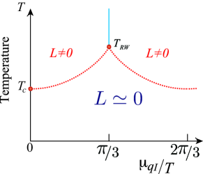
Figure 1: Schematical figure of Roberge-Weiss phase structure in the pure imaginary chemical potential regions.

Quark number density $n_{q}$ for $N_{f}$ degenerate quark flavours is defined by the following equation:

$$\frac{n_{q}}{T^{3}}=\frac{1}{VT^{2}}\frac{\partial}{\partial\mu_{q}}\ln Z_{GC}=\frac{N_{f}N_{t}^{3}}{N_{s}^{3}Z_{GC}}\int\mathcal{D}Ue^{-S_{G}}(\det\Delta(\mu_{q}))^{N_{f}}\mathrm{tr}\left[\Delta^{-1}\frac{\partial\Delta}{\partial\mu_{q}/T}\right].$$ (2)

It can be computed numerically for imaginary chemical potential. Note, that for the imaginary chemical potential $n_{q}$ is also purely imaginary: $n_{q}=in_{qI}$.

In this work we fitted $n_{qI}/T^{3}$ to theoretically motivated functions of $\mu_{qI}$. It is known that the density of noninteracting quark gas is described by

$$n_{q}/T^{3}=N_{f}\Bigl{(}\frac{\mu_{q}}{T}+\frac{1}{\pi^{2}}\Bigl{(}\frac{\mu_{q}}{T}\Bigr{)}^{3}\Bigr{)}.$$ (3)

We thus fit the data for $n_{qI}$ to an odd power polynomial of $\theta$

$$n_{qI}(\theta)/T^{3}=\sum_{n=1}^{n_{max}}a_{2n-1}\theta^{2n-1}\,,$$ (4)

in the deconfining phase at temperature $T>T_{RW}$. This type of the fit was also used in Refs. DElia:2009pdy ; Takahashi:2014rta ; Gunther:2016vcp ; Bornyakov:2016wld .

In the confining phase (below $T_{c}$) the hadron resonance gas model provides good description of the chemical potential dependence of thermodynamic observables Karsch:2003zq . Thus it is reasonable to fit the density to a Fourier expansion

$$n_{qI}(\theta)/T^{3}=\sum_{n=1}^{n_{max}}f_{3n}\sin(3n\theta)$$ (5)

Again this type of the fit was used in Refs. DElia:2009pdy ; Takahashi:2014rta and conclusion was made that it works well. We use both types of the fitting function in the deconfining phase at $T_{c}<T<T_{RW}$.

We made simulations of the lattice QCD with $N_{f}=2$ clover improved Wilson quarks and Iwasaki improved gauge field action. The more detailed definition of the lattice action can be found in Ref. Bornyakov:2016wld . The simulations were made on $16^{3}\times 4$ lattices. We obtained results at temperatures $T/T_{c}=1.35,1.20$, 1.08, and 1.035 in the deconfinement phase and $0.99,0.93,0.84$ in the confinement phase along the line of constant physics with $m_{\pi}/m_{\rho}=0.8$. We also present here our preliminary results for smaller quark mass with $m_{\pi}/m_{\rho}=0.65$ At this quark mass the simulations were made at $T/T_{c}=1.32,1.18,1.07,1.00,0.94,0.86$. The parameters of the action, including $c_{SW}$ value were borrowed from the WHOT-QCD collaboration paper Ejiri:2009hq . We compute the number density on samples of $N_{conf}$ configurations with $N_{conf}=1800$ or 3800, using every 10-th trajectory produced with Hybrid Monte Carlo algorithm.

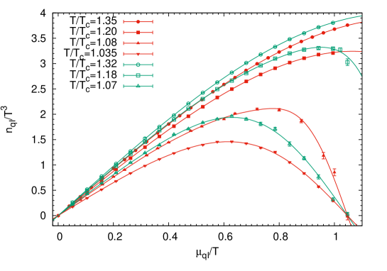
Figure 2: The quark number density $n_{qI}$ in the deconfinement phase at two quark masses: $m_{\pi}/m_{\rho}=0.8$ (filled symbols) and $m_{\pi}/m_{\rho}=0.65$ (empty symbols).

2 Quark number density

In this section we compare results for the quark number density obtained at the imaginary chemical potential for two values of the quark mass. In Figure 2 the data for the deconfinement phase are shown. One can see that at small values of $\mu_{qI}/T$ the number density for two quark masses differ only slightly for comparable values $T/T_{c}$. At the same time effects of the quark mass decreasing are quite visible in the range $\mu_{qI}/T>0.8$. As can be seen from Figure 3 in the confinement phase the differences between results for two quark masses might be mostly due to differences in the $T/T_{c}$ values.

This assumption is supported by comparison of the virial coefficients $f_{n}$ depicted in Figure 4. Note logarithmic scale for Y-axes in this Figure. From this Figure one can see an exponential decrease of $f_{n}$ with decreasing temperature. There is an indication of slower decrease for lower quark mass. Comparing the slopes for $f_{3}$ and $f_{6}$ we conclude that it is steeper for $f_{6}$.

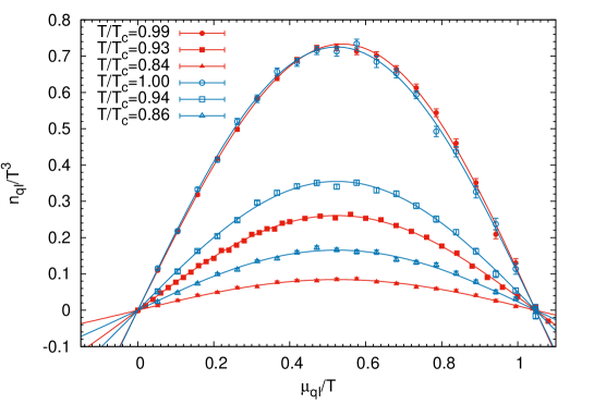
Figure 3: The quark number density $n_{qI}$ in the confinement phase at two quark masses: $m_{\pi}/m_{\rho}=0.8$ (filled symbols) and $m_{\pi}/m_{\rho}=0.65$ (empty symbols).

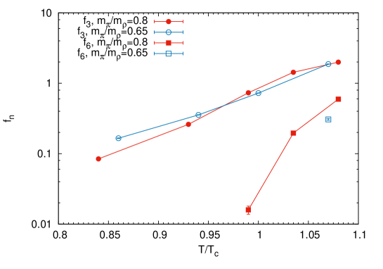
Figure 4: The virial coefficients $f_{3}$ and $f_{6}$ for $m_{\pi}/m_{\rho}=0.8$ (filled symbols) and $m_{\pi}/m_{\rho}=0.65$ (empty symbols).

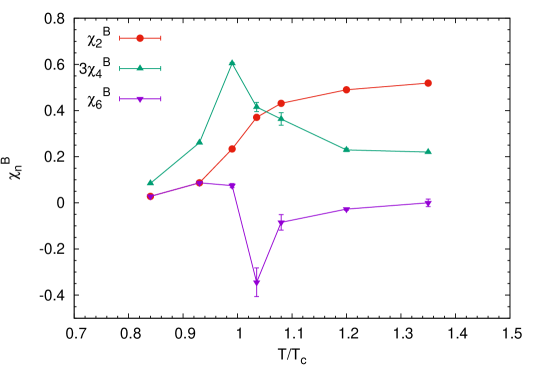
Figure 5: The generalized susceptibilities for $m_{\pi}/m_{\rho}=0.8$ .

3 Taylor expansion coefficients

The Taylor expansion coefficients for the pressure are introduced as follows:

$$\Delta P(T,\mu_{B})=\sum_{k=1}^{\infty}P_{2k}(T)\leavevmode\nobreak\ \mu_{B}^{2k}=\sum_{k=1}^{\infty}\frac{1}{(2k)!}\chi_{2k}(T)\leavevmode\nobreak\ \mu_{B}^{2k}\,,$$ (6)

where $\Delta P(T,\mu_{B})=P(T,\mu_{B})-P(T,0)$, $P_{2k}$ are Taylor expansion coefficients, $\chi_{2k}$ are called generalized susceptibilities. Before we discuss the Taylor expansion coefficients few comments about the fits follow. The fits to function eq. (5) are very stable with respect to change of the fitting range. This was observed for $T/T_{c}=0.84,0.93$. Since the statistical error for the coefficient $f_{3}$ is small at low temperatures we obtain the Taylor coefficients $a_{k}$ with low error even for high values of $k$. We should note that there is a source of uncertainty which we cannot estimate reliably. This is the contribution from the higher terms in the Fourier decomposition eq. (5). Our data indicate that for low temperatures $f_{6}$ is at least factor 100 smaller than $f_{3}$. This implies that for Taylor coefficients $a_{1}$ and $a_{3}$ the contribution from the second term in eq. (5) should be small while starting from $a_{5}$ this contribution might be substantial.

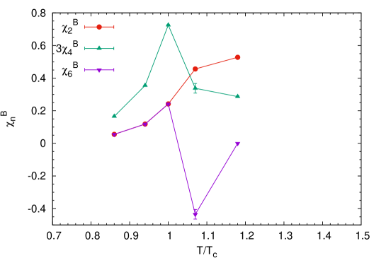
Figure 6: The generalized susceptibilities for $m_{\pi}/m_{\rho}=0.65$ .

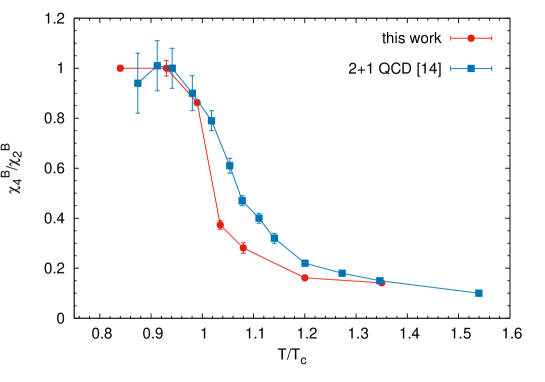
Figure 7: The ratio $\chi_{4}^{B}/\chi_{2}^{B}$ at $m_{\pi}/m_{\rho}=0.8$ in comparison with results from [14].

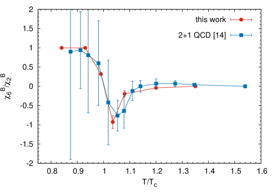
Figure 8: The ratio $\chi_{6}^{B}/\chi_{2}^{B}$ at $m_{\pi}/m_{\rho}=0.8$ in comparison with results from [14].

For consistency check of our results we also applied polynomial fit at low temperatures. The polynomial fit was applied for restricted range of $\mu_{qI}$ values. We obtained results compatible with respective Taylor coefficients $a_{k},k=1,3,5$ within error bars for $T/T_{c}=0.84,0.93$. For $T/T_{c}=1.035$ and 1.08 the results for $a_{k}$ obtained with two kind of fits are in agreement for $k=1$ only. We then used $a_{3}$ and $a_{5}$ values obtained from the polynomial fit. For the lighter quark mass we made similar computations.

The generalized susceptibilities $\chi_{n}$ for $n=2,4,6$ which are proportional to the Taylor coefficients $P_{n}$ are presented in Figure 5 for $m_{\pi}/m_{\rho}=0.8$ and in Figure 6 for $m_{\pi}/m_{\rho}=0.65$. We should note that our results for $P_{2}$ and $P_{4}$ are in agreement within error bars with results of Ref. Ejiri:2009hq where direct computation of the Taylor coefficients was done. But our error bars are substantially lower.

The Taylor coefficients were recently computed for the physical quark masses on lattices with small lattice spacing (and even in the continuum limit) in Refs. Gunther:2016vcp and Bazavov:2017dus . In Ref. Gunther:2016vcp the analytical continuation was used while in Ref Bazavov:2017dus direct method was employed. Results of these two computations were found to be in a good agreement Bazavov:2017dus . Our results presented in Figure 5 and Figure 6 are in good qualitative agreement with results of Refs. Gunther:2016vcp ; Bazavov:2017dus for all three susceptibilities. Quantitatively our results at $T>T_{c}$ are substantially higher what should be expected from the large lattice spacing effects estimated in Ref. Ejiri:2009hq .

In Figure 7 and Figure 8 we show the ratios $\chi_{4}^{B}/\chi_{2}^{B}$ and $\chi_{6}^{B}/\chi_{2}^{B}$, respectively. One can see that for these ratios our results are in very good agreement with results of Ref Bazavov:2017dus taken from their Figure 3. Substantial difference is observed only for $\chi_{4}^{B}/\chi_{2}^{B}$ at $1<T/T_{c}<1.1$. This agreement indicates that the finite lattice spacing effects are substantially cancelled in the ratios of the susceptibilities.

4 Conclusions

We computed the baryon number density and generalized susceptibilities $\chi_{n}$ in the lattice QCD with two flavors of Wilson fermions on $16^{3}\times 4$ lattices using analytical continuation. Comparing results for two quark masses we found that they do not differ substantially. Comparison of our results for the ratios $\chi_{4}^{B}/\chi_{2}^{B}$ and $\chi_{6}^{B}/\chi_{2}^{B}$ with results of Ref Bazavov:2017dus where simulations were done at the physical quark masses and small lattice spacing we found surprising agreement. This agreement indicates that our recent results Boyda:2017dyo showing agreement of cumulant ratios computed on the lattice with respective experimental results are not accidental.

Acknowledgments
This work was completed due to support by RSF grant under contract 15-12-20008. Computer simulations were performed on the FEFU GPU cluster Vostok-1 and MSU ’Lomonosov’ supercomputer.

References

- (1) J. Adams et al. (STAR), Nucl. Phys. A757, 102 (2005), nucl-ex/0501009
- (2) K. Aamodt et al. (ALICE), JINST 3, S08002 (2008)
- (3) S. Muroya, A. Nakamura, C. Nonaka, T. Takaishi, Prog. Theor. Phys. 110, 615 (2003), hep-lat/0306031
- (4) O. Philipsen, PoS LAT2005, 016 (2006), [PoSJHW2005,012(2006)], hep-lat/0510077
- (5) P. de Forcrand, PoS LAT2009, 010 (2009), 1005.0539
- (6) A. Roberge, N. Weiss, Nucl. Phys. B275, 734 (1986)
- (7) C. Bonati, P. de Forcrand, M. D’Elia, O. Philipsen, F. Sanfilippo, Phys. Rev. D90, 074030 (2014), 1408.5086
- (8) V. G. Bornyakov, D. L. Boyda, V. A. Goy, A. V. Molochkov, A. Nakamura, A. A. Nikolaev and V. I. Zakharov, Phys. Rev. D 95, no. 9, 094506 (2017) doi:10.1103/PhysRevD.95.094506 [arXiv:1611.04229 [hep-lat]].
- (9) M. D’Elia and F. Sanfilippo, Phys. Rev. D 80, 014502 (2009) doi:10.1103/PhysRevD.80.014502 [arXiv:0904.1400 [hep-lat]].
- (10) J. Takahashi, H. Kouno, M. Yahiro, Phys. Rev. D91, 014501 (2015), 1410.7518
- (11) J. Gunther, R. Bellwied, S. Borsanyi, Z. Fodor, S. D. Katz, A. Pasztor and C. Ratti, EPJ Web Conf. 137, 07008 (2017) doi:10.1051/epjconf/201713707008 [arXiv:1607.02493 [hep-lat]].
- (12) F. Karsch, K. Redlich, A. Tawfik, Phys. Lett. B571, 67 (2003), hep-ph/0306208
- (13) S. Ejiri, Y. Maezawa, N. Ukita, S. Aoki, T. Hatsuda, N. Ishii, K. Kanaya, T. Umeda (WHOT-QCD), Phys. Rev. D82, 014508 (2010), 0909.2121
- (14) A. Bazavov et al., Phys. Rev. D 95, no. 5, 054504 (2017)
- (15) D. Boyda, V. G. Bornyakov, V. Goy, A. Molochkov, A. Nakamura, A. Nikolaev and V. I. Zakharov, arXiv:1704.03980 [hep-lat].