Sharing Storage in a Smart Grid: A Coalitional Game Approach

Abstract

Sharing economy is a transformative socio-economic phenomenon built around the idea of sharing underused resources and services, e.g. transportation and housing, thereby reducing costs and extracting value. Anticipating continued reduction in the cost of electricity storage, we look into the potential opportunity in electrical power system where consumers share storage with each other. We consider two different scenarios. In the first scenario, consumers are assumed to already have individual storage devices and they explore cooperation to minimize the realized electricity consumption cost. In the second scenario, a group of consumers is interested to invest in joint storage capacity and operate it cooperatively. The resulting system problems are modeled using cooperative game theory. In both cases, the cooperative games are shown to have non-empty cores and we develop efficient cost allocations in the core with analytical expressions. Thus, sharing of storage in cooperative manner is shown to be very effective for the electric power system.

I Introduction

I-A Motivation

The sharing economy is disruptive and transformative socio-economic trend that has already impacted transportation and housing [1]. People rent out (rooms in) their houses and use their cars to provide transportation services. The business model of sharing economy leverages under utilized resources. Like these sectors, many of the resources in electricity grid is also under-utilized or under-exploited. There is potential benefit in sharing the excess generation by rooftop solar panels, sharing flexible demand, sharing unused capacity in the storage services, etc. Motivated by the recent studies [2] predicting a fast drop in battery storage prices, we focus on sharing electric energy storage among consumers.

I-B Literature Review

Storage prices are projected to decrease by more than $30\%$ by 2020. The arbitrage value and welfare effects of storage in electricity markets has been explored in literature. In [3], the value of storage arbitrage was studied in deregulated markets. In [4], the authors studied the role of storage in wholesale electricity markets. The economic viability of the storage elements through price arbitrage was examined in [5]. Agent-based models to explore the tariff arbitrage opportunities for residential storage systems were introduced in [6]. In [7, 8], authors address the optimal control and coordination of energy storage. All these works explore the economic value of storage to an individual, not for shared services. Sharing of storage among firms has been analyzed using non-cooperative game theory in [9]. But the framework needs a spot market among the consumers and also coordination is needed among the firms that are originally strategic.

In this paper, we explore sharing storage in a cooperative manner among consumers. Cooperative game theory has significant potential to model resource sharing effectively [10]. Cooperation and aggregation of renewable energy sources bidding in a two settlement market to maximize expected and realized profit has been analyzed using cooperative game theory in [11, 12, 13]. Under a cooperative set-up, the cost allocation to all the agents is a crucial task. A framework for allocating cost in a fair and stable way was introduced in [14]. Cooperative game theoretic analysis of multiple demand response aggregators in a virtual power plant and their cost allocation has been tackled in [15]. In [16], sharing opportunities of photovoltaic systems (PV) under various billing mechanisms were explored using cooperative game theory.

I-C Contributions and Paper Organization

In this paper, we investigate the sharing of storage systems in a time of use (TOU) price set-up using cooperative game theory. We consider two scenarios. In the first one, a group of consumers already own storage systems and they are willing to operate all together to minimize their electricity consumption cost. In a second scenario, a group of consumers wish to invest in a shared common storage system and get benefit for long term operation in a cooperative manner. We model both the cases using cooperative game theory. We prove that the resulting games developed have non-empty cores, i.e., cooperation is shown to be beneficial in both the cases. We also derive closed-form and easy to compute expressions for cost allocations in the core in both the cases. Our results suggest that sharing of electricity storage in a cooperative manner is an effective way to amortize storage costs and to increase its utilization. In addition, it can be very much helpful for consumers and at the same time to integrate renewables in the system, because off-peak periods correspond to large presence of renewables that can be stored for consumption during peak periods.

The remainder of the paper is organized as follows. In Section II, we formulate the cooperative storage problems. A brief review of cooperative game theory is presented in Section III. In Section IV, we state and explain our main results. A case study illustrating our results using real data from Pecan St. Project is presented in Section VI. Finally, we conclude the paper in Section VII.

II Problem Formulation

II-A System Model

We consider a set of consumers indexed by $i\in\mathcal{N}:=\{1,2,\ldots,N\}$. The consumers invest in storage. The consumers cooperate and share their storage with each other. We consider two scenarios here. In the scenario I, the consumers already have storage and they operate with storage devices connected to each other. In the scenario II, the consumers wish to invest in a common storage. There is a single meter for this group of consumers. We assume that there is necessary electrical connection between all the consumers for effective sharing. We ignore here the capacity constraints, topology or losses in the connecting network. The configuration of the scenarios with three consumers are depicted in Figure 1. Examples of the situations considered here include consumers in an industrial park, office buildings on a campus, or homes in a residential complex.

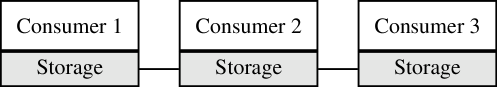
Figure 1: Configuration of three consumers in the two analyzed scenarios

II-B Cost of Storage

Each day is divided into two periods –peak and off-peak. There is a time-of-use pricing. The peak and off-peak period prices are denoted by $\pi_{h}$ and $\pi_{\ell}$ respectively. The prices are fixed and known to all the consumers.

Let $\pi_{i}$ be the daily capital cost of storage of the consumer $i\in\mathcal{N}$ amortized over its life span. Let the arbitrage price be defined by

$$\pi_{\delta}:=\pi_{h}-\pi_{\ell}$$ (1)

and define the arbitrage constant $\gamma_{i}$ as follows:

$$\gamma_{i}:=\frac{\pi_{\delta}-\pi_{i}}{\pi_{\delta}}$$ (2)

In order to have a viable arbitrage opportunity, we need

$$\pi_{i}\leq\pi_{\delta}$$ (3)

which corresponds to $\gamma_{i}\in[0,1]$. The consumers discharge their storage during peak hours and charge them during off-peak hours.

The daily cost of storage of a consumer $i\in\mathcal{N}$ for the peak period consumption $\mathbf{x}_{i}$ depends on the capacity investment $C_{i}$ and is given by

$$J(\mathbf{x}_{i},C_{i})=\pi_{i}C_{i}+\pi_{h}(\mathbf{x}_{i}-C_{i})^{+}+\pi_{\ell}\min\{C_{i},\mathbf{x}_{i}\},$$ (4)

where $\pi_{i}C_{i}$ is the capital cost of acquiring $C_{i}$ units of storage capacity, $\pi_{h}(\mathbf{x}_{i}-C_{i})^{+}$ is the daily cost of the electricity purchase during peak price period, and $\pi_{\ell}\min\{\mathbf{x}_{i},C_{i}\}$ is the daily cost of the electricity purchase during off-peak period to be stored for consumption during the peak period. We ignore the off-peak period electricity consumption of the consumer from the expression of $J$ as its expression is independent of the storage capacity. The daily peak consumption of electricity is not known in advance and we assume it to be a random variable. Let $F$ be the joint cumulative distribution function (CDF) of the collection of random variables $\{\mathbf{x}_{i}:i\in\mathcal{N}\}$ that represents the consumptions of the consumers in $\mathcal{N}$. If $\mathcal{S}\subseteq\mathcal{N}$ is a subset of consumers, then $\mathbf{x}_{\mathcal{S}}$ denotes the aggregated peak consumption of $\mathcal{S}$ and its CDF is $F_{\mathcal{S}}$.

The daily cost of storage of a group of consumers $\mathcal{S}\subseteq\mathcal{N}$ with aggregated peak consumption $\mathbf{x}_{\mathcal{S}}=\sum_{i\in\mathcal{S}}\mathbf{x}_{i}$ and joint storage capacity $C_{\mathcal{S}}$ is

$$J(\mathbf{x}_{\mathcal{S}},C_{\mathcal{S}})=\pi_{\mathcal{S}}C_{\mathcal{S}}+\pi_{h}(\mathbf{x}_{\mathcal{S}}-C_{\mathcal{S}})^{+}+\pi_{\ell}\min\{C_{\mathcal{S}},\mathbf{x}_{\mathcal{S}}\}$$ (5)

where $\pi_{S}$ is the daily capital cost of aggregated storage of the group amortized during its life span. Note that the individual storage costs (4) are obtained from (5) for the singleton sets $\mathcal{S}=\{i\}$.

The daily cost of storage given by (4) and (5) are random variables with expected values

$$J_{\mathcal{S}}(C_{\mathcal{S}})=\mathbb{E}J_{\mathcal{S}}(\mathbf{x}_{\mathcal{S}},C_{\mathcal{S}}),\quad\mathcal{S}\subseteq\mathcal{N}.$$ (6)

In the sequel, we will distinguish between the random variables and their realized values by using bold face fonts $\mathbf{x}_{\mathcal{S}}$ for the random variables and normal fonts $x_{\mathcal{S}}$ for their realized values.

II-C Quantifying the Benefit of Cooperation Benefit

We are interested in studying and quantifying the benefit of cooperation in the two scenarios. In the first scenario, the consumers already have installed storage capacity $\{C_{i}:i\in\mathcal{N}\}$ that they acquired in the past. Each of the consumers can have a different storage technology that was acquired at a different time compared to the other consumers. Consequently, each consumer has a different daily capital cost $\pi_{i}$. The consumers aggregate their storage capacities and they operate using the same strategy, they use the aggregated storage capacity to store energy during off-peak periods that they will later use during peak periods. By aggregating storage devices, the unused capacity of some consumers is used by others producing cost savings for the group. We analyze this scenario using cooperative game theory and develop an efficient allocation rule of the daily storage cost that is satisfactory for every consumer.

In the second scenario, we consider a group of consumers that join to buy storage capacity that they want to use in a cooperative way. First, the group of consumers have to make a decision about how much storage capacity they need to acquire and then they have to share the expected cost among the group participants. The decision problem is modeled as an optimization problem where the group of consumers minimize the expected cost of daily storage. The problem of sharing the expected cost is modeled using cooperative game theory. We quantify the reduction in the expected cost of storage for the group and develop a mechanism to allocate the expected cost among the participants that is satisfactory for all of them.

III Background: Coalitional Game Theory for Cost Sharing

Game theory deals with rational behavior of economic agents in a mutually interactive setting [17]. Broadly speaking, there are two major categories of games: non-cooperative games and cooperative games. Cooperative games (or coalitional games) have been used extensively in diverse disciplines such as social science, economics, philosophy, psychology and communication networks [18, 10]. Here, we focus on cooperative games for cost sharing [19].

Let $\mathcal{N}:=\{1,2,\ldots,N\}$ denote a finite collection of players. In a cooperative game for cost sharing, the players want to minimize their joint cost and share the resulting cost cooperatively.

Definition 1 (Coalition)

A coalition is any subset $\mathcal{S}\subseteq\mathcal{N}$. The number of players in a coalition $\mathcal{S}$ is denoted by its cardinality, $|\mathcal{S}|$. The set of all possible coalitions is defined as the power set $2^{\mathcal{N}}$ of $\mathcal{N}$. The grand coalition is the set of all players, $\mathcal{N}$.

Definition 2 (Game and Value)

A cooperative game is defined by a pair $(\mathcal{N},v)$ where $v:2^{\mathcal{N}}\rightarrow\mathbb{R}$ is the value function that assigns a real value to each coalition $\mathcal{S}\subseteq\mathcal{N}$. Hence, the value of coalition $\mathcal{S}$ is given by $v(\mathcal{S})$. For the cost sharing game, $v(\mathcal{S})$ is the total cost of the coalition.

Definition 3 (Subadditive Game)

A cooperative game $(\mathcal{N},v)$ is subadditive if, for any pair of disjoint coalitions $\mathcal{S},\mathcal{T}\subset\mathcal{N}$ with $\mathcal{S}\cap\mathcal{T}=\emptyset$, we have $v(\mathcal{S})+v(\mathcal{T})\ \geq\ v(\mathcal{S}\cup\mathcal{T}).$

Here we consider the value of the coalition $v(\mathcal{S})$ is transferable among players. The central question for a subadditive cost sharing game with transferrable value is how to fairly distribute the coalition value among the coalition members.

Definition 4 (Cost Allocation)

A cost allocation for the coalition $\mathcal{S}\subseteq\mathcal{N}$ is a vector $x\in\mathbb{R}^{N}$ whose entry $x_{i}$ represents the allocation to member $i\in\mathcal{S}$ ($x_{i}=0,\ \ i\notin\mathcal{S}$).

For any coalition $\mathcal{S}\subseteq{\mathcal{N}}$, let $x_{\mathcal{S}}$ denote the sum of cost allocations for every coalition member, i.e. $x_{\mathcal{S}}=\sum_{i\in\mathcal{S}}x_{i}$.

Definition 5 (Imputation)

A cost allocation $x$ for the grand coalition $\mathcal{N}$ is said to be an imputation if it is simultaneously efficient –i.e. $v(\mathcal{N})=x_{\mathcal{N}}$, and individually rational –i.e. $v({i})\geq x_{i},\forall i\in\mathcal{N}$. Let $\mathcal{I}$ denote the set of all imputations.

The fundamental solution concept for cooperative games is the core [17].

Definition 6 (The Core)

The core $\mathcal{C}$ for the cooperative game $(\mathcal{N},v)$ with transferable cost is defined as the set of cost allocations such that no coalition can have cost which is lower than the sum of the members current costs under the given allocation.

$$\mathcal{C}:=\left\{x\in\mathcal{I}:v(\mathcal{S})\geq x_{\mathcal{S}},\forall\mathcal{S}\in 2^{\mathcal{N}}\right\}.$$ (7)

A classical result in cooperative game theory, known as Bondareva-Shapley theorem, gives a necessary and sufficient condition for a game to have nonempty core. To state this theorem, we need the following definition.

Definition 7 (Balanced Game and Balanced Map)

A cooperative game $(\mathcal{N},v)$ for cost sharing is balanced if for any balanced map $\alpha$, $\sum_{\mathcal{S}\in 2^{\mathcal{N}}}\alpha(\mathcal{S})v(\mathcal{S})\geq v(\mathcal{N})$ where the map $\alpha:2^{\mathcal{N}}\rightarrow[0,1]$ is said to be balanced if for all $i\in\mathcal{N}$, we have $\sum_{\mathcal{S}\in 2^{\mathcal{N}}}\alpha(\mathcal{S})\mathbf{1}_{\mathcal{S}}(i)=1$, where $\mathbf{1}_{\mathcal{S}}$ is the indicator function of the set $\mathcal{S}$, i.e. $\mathbf{1}_{\mathcal{S}}(i)=1$ if $i\in\mathcal{S}$ and $\mathbf{1}_{\mathcal{S}}(i)=0$ if $i\not\in\mathcal{S}$.

Next we state the Bondareva-Shapley theorem.

Theorem 1 (Bondareva-Shapley Theorem [10])

A coalitional game has a nonempty core if and only if it is balanced.

If a game is balanced, the nucleolus [18] is a solution that is always in the core.

IV Main Results

IV-A Scenario I: Realized Cost Minimization with Already Procured Storage Elements

Our first concern is to study if there is some benefit in cooperation of the consumers by sharing the storage capacity that they already have. To analyze this scenario we shall formulate our problem as a coalitional game.

IV-A1 Coalitional Game and Its Properties

The players of the cooperative game are the consumers that share their storage and want to reduce their realized joint storage investment cost. For any coalition $\mathcal{S}\subseteq\mathcal{N}$, the cost of the coalition is $u(\mathcal{S})$ which is the realized cost of the joint storage investment $C_{\mathcal{S}}=\sum_{i\in\mathcal{S}}C_{i}$. Each consumer may have a different daily capital cost of storage $\{\pi_{i}:i\in\mathcal{N}\}$, because they did not necessarily their storage systems at the same time or at the same price for KW. The realized cost of the joint storage for the peak period consumption $x_{\mathcal{S}}=\sum_{i\in\mathcal{S}}x_{i}$ is given by

$$u(\mathcal{S}) =J(x_{\mathcal{S}},C_{\mathcal{S}})$$ (8)

where $J$ was defined in (5). Since we are using the realized value of the aggregated peak consumption $x_{\mathcal{S}}$, $J(x_{\mathcal{S}},C_{\mathcal{S}})$ is not longer a random variable.

In order to show that cooperation is advantageous for the members of the group, we have to prove that the game is subadditive. In such a case, the joint daily investment cost of the consumers is never greater that the sum of the individual daily investment costs. Subadditivity of the cost sharing coalitional game is established in Theorem 2.

Theorem 2

The cooperative game for storage investment cost sharing $(\mathcal{N},u)$ with the cost function $u$ defined in (8) is subadditive.

Proof

See appendix.

However, subadditivity is not enough to provide satisfaction of the coalition members. We need a stabilizing allocation mechanism of the aggregated cost. Under a stabilizing cost sharing mechanism no member in the coalition is impelled to break up the coalition. Such a mechanism exists if the cost sharing coalitional game is balanced. Balancedness of the cost sharing coalitional game is established in Theorem 3.

Theorem 3

The cooperative game for storage investment cost sharing $(\mathcal{N},u)$ with the cost function $u$ defined in (8) is balanced.

Proof

See the appendix.

IV-A2 Sharing of Realized Cost

Since the cost sharing cooperative game $(\mathcal{N},u)$ is balanced, its core is nonempty and there always exist cost allocations that stabilize the grand coalition. One of this coalitions is the nucleolus while another one is the allocation that minimizes the worst case excess [12]. However, computing these allocations requires solving linear programs with a number of constraints that grows exponentially with the cardinality of the grand coalition and they can be only applied for coalitions of moderate size. As an alternative to these computationally intensive cost allocations, we propose the following cost allocation.

Allocation 1

Define the cost allocation $\{\xi_{i}:i\in\mathcal{N}\}$ as follows:

$$\xi_{i}:=\left\{\begin{array}[]{ll}\pi_{i}C_{i}+\pi_{h}(x_{i}-C_{i})+\pi_{\ell}C_{i},&\mathrm{if}\ x_{\mathcal{N}}\geq C_{\mathcal{N}}\\ \pi_{i}C_{i}+\pi_{\ell}x_{i},&\mathrm{if}\ x_{\mathcal{N}}<C_{\mathcal{N}}\end{array}\right.$$ (11)

for all $i\in\mathcal{N}$.

We establish in Theorem 4, this cost allocation belongs to the core of the cost sharing cooperative game.

Theorem 4

The cost allocation $\{\xi_{i}:i\in\mathcal{N}\}$ defined in Allocation 1 belongs to the core of the cost sharing cooperative game $(\mathcal{N},u)$.

Proof

See appendix.

Unlike the nucleolus or the cost allocation minimizing the worst-case excess, Allocation 1 has an analytical expression and can be easily obtained without any costly computation. Thus, we have developed a strategy such that consumers that independently invested in storage, and are subject to a two period (peak and off-peak) TOU pricing mechanism can reduce their costs by sharing their storage devices. Moreover, we have proposed a cost sharing allocation rule that stabilizes the grand coalition. This strategy can be considered a weak cooperation because each consumer acquired its storage capacity independently of each other, but they agree to share the joint storage capacity.

In the next section we consider a stronger cooperation problem, where a group of consumers decide to invest jointly in storage capacity.

IV-B Scenario II: Expected Cost Minimization for Joint Storage Investment

In this scenario, we consider a group of consumers indexed by $i\in\mathcal{N}$, that decide to jointly invest in storage capacity. We are interested in studying whether cooperation provides a benefit for the coalition members for the long term.

IV-B1 Coalitional Game and Its Properties

Similar to the previous case, only the peak consumption is relevant in the investment decision. Let $\mathbf{x}_{i}$ denote the daily peak period consumption of consumer $i\in\mathcal{N}$. Unlike the previous scenario, here $\mathbf{x}_{i}$ is a random variable with marginal cumulative distribution function (CDF) $F_{i}$. The daily cost of the consumer $i\in\mathcal{N}$ depends on the storage capacity investment of the consumer as per (4). This cost is also a random variable. If the consumer is risk neutral, it acquires the storage capacity $C_{i}^{*}$ that minimizes the expected value of the daily cost

$$C_{i}^{*} =\arg\min_{C_{i}\geq 0}J_{i}(C_{i}),$$ (12)

where

$$J_{i}(C_{i}) =\mathbb{E}J(\mathbf{x}_{i},C_{i}),$$ (13)

and $\pi_{\mathcal{S}}$ is the daily capital cost of storage amortized over its lifespan that in this case is the same for each of the consumers –i.e. $\pi_{i}=\pi_{\mathcal{S}}$ for all $i\in\mathcal{N}$, because we assume that they buy storage devices of the same technology at the same time. This problem has been previously solved in [9] and its solution is given by Theorem 5.

Theorem 5 ([9])

The storage capacity of a consumer $i\in\mathcal{N}$ that minimizes its daily expected cost is $C^{*}_{i}$, where

$$F_{i}(C^{*}_{i})=\frac{\pi_{\delta}-\pi_{\mathcal{S}}}{\pi_{\delta}}=\gamma_{\mathcal{S}}$$

and the resulting optimal cost is

$$J^{*}_{i}=J_{i}(C^{*}_{i})=\pi_{\ell}\mathbb{E}[\mathbf{x}_{i}]+\pi_{\mathcal{S}}\mathbb{E}[\mathbf{x}_{i}\mid\mathbf{x}_{i}\geq C_{i}^{*}].$$ (14)

Let us consider a group of consumers $\mathcal{S}\subseteq N$ that decide to join to invest in joint storage capacity. The joint peak consumption of the coalition is $\mathbf{x}_{\mathcal{S}}=\sum_{i\in\mathcal{S}}\mathbf{x}_{i}$ with CDF $F_{\mathcal{S}}$. We also assume that the joint CDF of all the agent’s peak consumptions $F$ is known or can be estimated from historical data. By applying Theorem 5, the optimal investment in storage capacity of the coalition $\mathcal{S}\subseteq\mathcal{N}$ is $C_{\mathcal{S}}^{*}$ such that $F_{\mathcal{S}}(C_{\mathcal{S}}^{*})=\gamma_{\mathcal{S}}$ and the optimal cost is

$$J_{\mathcal{S}}^{*}=J_{\mathcal{S}}(C_{\mathcal{S}}^{*})=\pi_{\ell}\mathbb{E}[\mathbf{x}_{\mathcal{S}}]+\pi_{\mathcal{S}}\mathbb{E}[\mathbf{x}_{\mathcal{S}}\mid\mathbf{x}_{\mathcal{S}}\geq C_{\mathcal{S}}^{*}].$$ (15)

Consider the cost sharing cooperative game $(\mathcal{N},v)$ where the cost function $v:2^{\mathcal{N}}\rightarrow\mathbb{R}$ is defined as follows

$$v(\mathcal{S})=J_{\mathcal{S}}^{*}=\arg\min_{C_{\mathcal{S}}\geq 0}J_{\mathcal{S}}(C_{\mathcal{S}}),$$ (16)

where $J_{\mathcal{S}}^{*}$ was defined in (15).

Similar to the case of consumers that already own storage capacity and decide to join to reduce their costs, here we prove that the cooperative game is subadditive so that the consumer obtain a reduction of cost. This is the result in Theorem 6.

Theorem 6

The cooperative game for storage investment cost sharing $(\mathcal{N},v)$ with the cost function $v$ defined in (16) is subadditive.

Proof

See appendix.

We also need a cost allocation rule that is stabilizing. Theorem 7 establishes that the game is balanced and has a stabilizing allocation.

Theorem 7

The cooperative game for storage investment cost sharing $(\mathcal{N},v)$ with the cost function $v$ defined in (16) is balanced.

Proof

See appendix.

IV-B2 Stable Sharing of Expected Cost

Similar to the previous scenario, we were able to develop a cost allocation rule that is in the core. This cost allocation rule has an analytical formula and can be efficiently computed. This allocation rule is defined as follows.

Allocation 2

Define the cost allocation $\{\zeta_{i}:i\in\mathcal{N}\}$ as follows:

$$\zeta_{i}:=\pi_{\ell}\mathbb{E}[\mathbf{x}_{i}]+\pi_{\mathcal{S}}\mathbb{E}[\mathbf{x}_{i}\mid\mathbf{x}_{\mathcal{N}}\geq C^{*}_{\mathcal{N}}],\ i\in\mathcal{N}.$$ (17)

In the next theorem, we prove that Allocation 2 provides a sharing mechanism of the expected daily storage cost of a coalition of agents that is in the core of the cooperative game.

Theorem 8

The cost allocation $\{\zeta_{i}:i\in\mathcal{N}\}$ defined in Allocation 2 belongs to the core of the cost sharing cooperative game $(\mathcal{N},v)$.

Proof

See appendix.

IV-B3 Sharing of Realized Cost

Based on the above results, the consumers can invest on joint storage and they will make savings for long term. But the cost allocation $\zeta_{i}$ defined by (17) is in expectation. The realized allocation will be different due to the randomness of the daily consumption. Here we develop a daily cost allocation for the $k$-th day as

$$\rho_{i}^{k}=\beta_{i}\pi^{k}_{\mathcal{N}},$$ (18)

where $\pi^{k}_{\mathcal{N}}$ is the realized cost for the grand coalition on the $k$-th day and $\beta_{i}=\frac{\zeta_{i}}{\sum_{i=1}^{N}\zeta_{i}}$.

As $\sum_{i=1}^{N}\beta_{i}=1$, $\sum_{i=1}^{N}\rho_{i}^{k}=\pi^{k}_{\mathcal{N}}$ and the cost allocation is budget balanced. Also using strong law of large numbers, $\frac{1}{K}\sum_{k=1}^{K}\rho^{k}_{i}\rightarrow\zeta_{i}$ as $K\rightarrow\infty$ and the realized allocation is strongly consistent with the fixed allocation $\zeta_{i}$.

V Benefit of Cooperation

V-A Scenario I

The benefit of cooperation by joint operation of storage reflected in the total reduction of cost is given by

$$\sum_{i\in\mathcal{S}} J_{i}-J_{S}=\pi_{h}(\sum_{i\in\mathcal{S}}(x_{i}-C_{i})^{+}-(x_{\mathcal{S}}-C_{\mathcal{S}})^{+})+$$

$$\pi_{\ell}(\sum_{i\in\mathcal{S}}\min\{C_{i},x_{i}\}-\min\{C_{\mathcal{S}},x_{\mathcal{S}}\}),$$ (19)

where the reduction for individual agent with cost allocation (11) is

$$J_{i}-\zeta_{i}:=\left\{\begin{array}[]{ll}\pi_{\delta}(C_{i}-x_{i})^{+},&\mathrm{if}\ x_{\mathcal{N}}\geq C_{\mathcal{N}}\\ \pi_{\delta}(x_{i}-C_{i})^{+},&\mathrm{if}\ x_{\mathcal{N}}<C_{\mathcal{N}}\end{array}\right.$$ (22)

V-B Scenario II

The benefit of cooperation given by the reduction in the expected cost that the coalition $\mathcal{S}$ obtains by jointly acquiring and exploiting the storage is

$$\sum_{i\in\mathcal{S}} J_{i}^{*}-J_{\mathcal{S}}^{*}=$$

$$\pi_{\mathcal{S}}\sum_{i\in\mathcal{S}}\mathbb{E}[\mathbf{x}_{i}\mid\mathbf{x}_{i}\geq C_{i}^{*}]-\pi_{\mathcal{S}}\mathbb{E}[\mathbf{x}_{\mathcal{S}}\mid\mathbf{x}_{\mathcal{S}}\geq C_{\mathcal{S}}^{*}],$$ (23)

and the reduction in expected cost of each participant assuming that the expected cost of the coalition is split using cost allocation (17) is

$$J_{i}^{*}-\zeta_{i}=\pi_{\mathcal{S}}\mathbb{E}[\mathbf{x}_{i}\mid\mathbf{x}_{i}\geq C_{i}^{*}]-\pi_{\mathcal{S}}\mathbb{E}[\mathbf{x}_{i}\mid\mathbf{x}_{\mathcal{S}}\geq C_{\mathcal{S}}^{*}].$$ (24)

VI Case Study

We develop a case study to illustrate our results. For this case study, we used data from the Pecan St project [20]. We consider a two-period ToU tariff with $\pi_{h}=55$¢/KWh, and $\pi_{\ell}=20$¢/KWh. Electricity storage is currently expensive. The amortized cost of Tesla’s Powerwall Lithium-ion battery is around 25¢/KWh per day. But storage prize is projected to reduce by $30\%$ by 2020 [21]. Keeping in mind this projection, we consider $\pi_{\mathcal{S}}=15$¢/KWh.

A group of five household decide to join to acquire storage. Using historical data of 2016, we estimate the individual CDFs of their daily peak consumptions and the CDF of the daily joint peak consumption. Peak consumption period in Texas corresponds to non-holidays and non-weekends from 7h to 23h. The estimated CDFs for peak consumption are depicted in Figure 2. From this figure, we can see that the shape of the CDFs are quite similar for the five households. The correlation coefficients of these five households are given in Table I. Although the shape of the CDFs are very similar, the peak consumptions are not completely dependent. This means that there is room for reduction in cost by making a coalition. The optimal investments in storage for the five households and for the grand coalition are given in Table II. Also in this table, we show the allocation of the expected storage cost given by (17). The reduction in cost for the consumers coalition is about 5%, however those with less correlation with the other, have a larger reduction. Consumers 3 and 4 have cost reductions higher than 7%, while consumer 1, whose consumption is more correlated with the other, have about 2.4% of cost reduction.

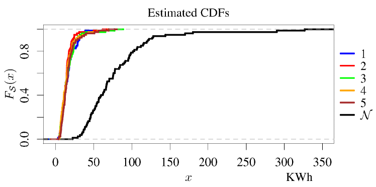
Figure 2: Estimated CDFs of the peak consumption of the five households and their aggregated consumption

TABLE I: Correlation coefficients for the five households

	1	2	3	4	5
1	1.000000	0.363586	0.297733	0.292073	0.486665
2	0.363586	1.000000	0.132320	0.453056	0.157210
3	0.297733	0.132320	1.000000	0.085868	0.365212
4	0.292073	0.453056	0.085869	1.000000	-0.056696
5	0.486665	0.157210	0.365212	-0.056696	1.000000

TABLE II: Optimal storage capacity investments (in KWh), minimal expected storage cost (in $) and expected cost allocation of the grand coalition (in $)

	$1$	$2$	$3$	$4$	$5$	$\mathcal{N}$
$C_{i}^{*}$	22.98	14.09	12.64	13.21	29.82	95.58
$J_{i}^{*}$	899.76	579.79	600.88	525.51	1189.41	3604.13
$\zeta_{i}$	882.45	543.10	550.02	488.20	1140.35	3604.13

Now, we assume that the five households buy storage independently and then decide to cooperate by sharing their storage to reduce the realized cost. This corresponds to Scenario I. For simplicity of computation and comparison with scenario II, we consider $\pi_{i}=\pi_{S}$ for all $i$. The realized cost is allocated using (11). In Table III, we show the allocation of the realized aggregated cost for the ten first days of 2016, assuming that the households have storage capacities $\{C_{i}^{*}:i\in\mathcal{N}\}$.

TABLE III: Allocation of the realized cost for Scenario I for the first ten days of the year (in $)

Day	$\xi_{1}$	$\xi_{2}$	$\xi_{3}$	$\xi_{4}$	$\xi_{5}$
1	492.66	612.83	436.88	549.61	904.69
2	464.89	624.96	343.61	567.21	947.27
3	541.21	482.61	299.84	541.40	820.46
4	675.74	373.95	377.64	418.01	734.10
5	761.41	403.49	405.52	371.64	799.23
6	646.05	516.53	404.89	573.17	812.54
7	654.47	760.99	387.80	536.92	797.46
8	583.59	411.25	533.00	455.56	831.97
9	640.46	394.04	482.85	483.24	787.20
10	604.49	446.14	475.46	310.22	791.60

Finally, in Figure 3, we depict the evolution of the average allocation of the realized cost of storage to each household for the 2016 year. The average allocation for $D$ days is given by

$$\bar{\xi}_{i}(D)=\frac{1}{D}\sum_{i=1}^{D}\xi_{i},\ i\in\mathcal{N},$$ (25)

where $D$ is the number of days. The average cost allocation is compared to the optimal expected costs $J_{i}^{*}$. Assuming stationarity of the peak consumptions random variables, the expected allocation converge to some values $\xi_{i}^{\infty}=\lim_{D\rightarrow\infty}\bar{\xi}_{i}(D)\leq J_{i}^{*}$ for $i\in\mathcal{N}$, as it is shown in Figure 3.

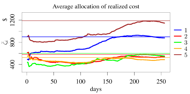
Figure 3: Average allocation of the realized storage cost

VII Conclusions

In this paper, we explored sharing opportunities of electricity storage elements among a group of consumers. We used cooperative game theory as a tool for modeling. Our results prove that cooperation is beneficial for agents that either already have storage capacity or want to acquire storage capacity. In the first scenario, the different agents only need the infrastructure to share their storage devices. In such a case the operative scheme is really simple, because each agent only has to storage at off-peak periods as much as possible energy that they will consume during peak periods. At the end of the day, the realized cost is shared among the participants. In the second scenario, the coalition members can take an optimal decision about how much capacity they jointly acquire by minimizing the expected daily storage cost. We showed that the cooperative games in both the cases are balanced. We also developed allocation rules with analytical formulas in both the cases. Thus, our results suggest that sharing of storage in a cooperative way is very much useful for all the agents and the society.

Appendix A Proofs

A-A Proof of Theorem 2

We shall prove that $J$ defined by (4) is a subadditive function. For any nonnegative real numbers $x_{\mathcal{S}}$, $x_{\mathcal{T}}$, $C_{\mathcal{S}}$, $C_{\mathcal{T}}$, we define $J_{\mathcal{S}}=J(x_{\mathcal{S}},C_{\mathcal{S}})$, $J_{\mathcal{T}}=J(x_{\mathcal{T}},C_{\mathcal{T}})$, $J_{\mathcal{S}\cup\mathcal{T}}=J(x_{\mathcal{S}}+x_{\mathcal{T}},C_{\mathcal{S}}+C_{\mathcal{T}})$, then

$$J_{\mathcal{S}} =\sum_{i\in\mathcal{S}}\pi_{i}C_{i}+\pi_{h}(x_{\mathcal{S}}-C_{\mathcal{S}})^{+}+\pi_{\ell}\min\{C_{\mathcal{S}},x_{\mathcal{S}}\},$$

$$J_{\mathcal{T}} =\sum_{i\in\mathcal{T}}\pi_{i}C_{i}+\pi_{h}(x_{\mathcal{T}}-C_{\mathcal{T}})^{+}+\pi_{\ell}\min\{C_{\mathcal{T}},x_{\mathcal{T}}\},$$

$$J_{\mathcal{S}\cup\mathcal{T}} =\sum_{i\in\mathcal{S}\cup\mathcal{T}}\pi_{i}C_{i}+\pi_{h}(x_{\mathcal{S}}+x_{\mathcal{T}}-C_{\mathcal{S}}-C_{\mathcal{T}})^{+}+$$

$$\qquad\pi_{\ell}\{C_{\mathcal{S}}+C_{\mathcal{T}},x_{\mathcal{S}}+x_{\mathcal{T}}\}.$$

We can distinguish four cases: (a) $x_{\mathcal{S}}\geq C_{\mathcal{S}}$ and $x_{\mathcal{T}}\geq C_{\mathcal{T}}$, (b) $x_{\mathcal{S}}\geq C_{\mathcal{S}}$, $x_{\mathcal{T}}<C_{\mathcal{T}}$ and $x_{\mathcal{S}}+x_{\mathcal{T}}\geq C_{\mathcal{S}}+C_{\mathcal{T}}$, (c) $x_{\mathcal{S}}\geq C_{\mathcal{S}}$, $x_{\mathcal{T}}<C_{\mathcal{T}}$ and $x_{\mathcal{S}}+x_{\mathcal{T}}<C_{\mathcal{S}}+C_{\mathcal{T}}$, and (d) $x_{\mathcal{S}}<C_{\mathcal{S}}$ and $x_{\mathcal{T}}<C_{\mathcal{T}}$. Using simple algebra it is easy to see that for all of these cases, $J_{\mathcal{S}\cup\mathcal{T}}\leq J_{\mathcal{S}}+J_{\mathcal{T}}$ or equivalently,

$$J(x_{\mathcal{S}}+x_{\mathcal{T}},C_{\mathcal{S}}+C_{\mathcal{T}})\leq J(x_{\mathcal{S}},C_{\mathcal{S}})+J(x_{\mathcal{T}},C_{\mathcal{T}}),$$ (26)

and this proves subadditivity of $J$. Since the storage cost function $u(\mathcal{S})=J(x_{\mathcal{S}},C_{\mathcal{S}})$, the cost sharing cooperative game $(\mathcal{N},u)$ is subadditive. ∎

A-B Proof of Theorem 3

We notice that the function $J$ is positive homogeneous, i.e, for any $\alpha\geq 0$, $J(\alpha x_{\mathcal{S}},\alpha C_{\mathcal{S}})=\alpha J(x_{\mathcal{S}},C_{\mathcal{S}}).$ $J$ is also subadditive as per Theorem 2. Thus for any arbitrary balanced map $\alpha:2^{\mathcal{N}}\rightarrow[0,1]$

$$\sum_{\mathcal{S}\in 2^{\mathcal{N}}} \alpha(\mathcal{S})u(\mathcal{S})$$

$$=\sum_{\mathcal{S}\in 2^{\mathcal{N}}}\alpha(\mathcal{S})J(x_{\mathcal{S}},C_{\mathcal{S}})$$

$$=\sum_{\mathcal{S}\in 2^{\mathcal{N}}}J(\alpha(\mathcal{S})x_{\mathcal{S}},\alpha(\mathcal{S})C_{\mathcal{S}})\ \text{[positive homogeneity]}$$

$$\geq J(\sum_{\mathcal{S}\in 2^{\mathcal{N}}}\alpha(\mathcal{S})x_{\mathcal{S}},\sum_{\mathcal{S}\in 2^{\mathcal{N}}}\alpha(\mathcal{S})C_{\mathcal{S}})\ \text{[subadditivity]}$$

$$=J(\sum_{i\in\mathcal{N}}\sum_{\mathcal{S}\in 2^{\mathcal{N}}}\alpha(\mathcal{S})\mathbf{1}_{\mathcal{S}}(i)x_{\mathcal{S}},\sum_{i\in\mathcal{N}}\sum_{\mathcal{S}\in 2^{\mathcal{N}}}\alpha(\mathcal{S})\mathbf{1}_{\mathcal{S}}(i)C_{\mathcal{S}})$$

$$=J(x_{\mathcal{N}},C_{\mathcal{N}})=u(\mathcal{N}).$$

and this proves that the cost sharing game $(\mathcal{N},u)$ is balanced. ∎

A-C Proof of Theorem 4

We begin by proving that the cost allocation (11) is an imputation, i.e. $\xi\in\mathcal{I}$. An imputation is a cost allocation satisfying budget balance and individual rationality.

If $x_{\mathcal{N}}\geq C_{\mathcal{N}}$:

$$\sum_{i\in\mathcal{N}}\xi_{i} =\sum_{i\in\mathcal{N}}\pi_{i}C_{i}+\pi_{h}(x_{\mathcal{N}}-C_{\mathcal{N}})+\pi_{\ell}C_{\mathcal{N}}=u(\mathcal{N}).$$

If $x_{\mathcal{N}}<C_{\mathcal{N}}$:

$$\sum_{i\in\mathcal{N}}\pi_{i}C_{i}+\pi_{\ell}x_{\mathcal{N}}=u(\mathcal{N}).$$

Thus, $\sum_{i\in\mathcal{N}}\xi_{i}=u(\mathcal{N})$ and the cost allocation $\{\xi_{i}:i\in\mathcal{N}\}$ satisfies budget balance.

The individual cost is:

$$u(\{i\}) =\left\{\begin{array}[]{ll}\pi_{i}C_{i}+\pi_{h}(x_{i}-C_{i})+\pi_{\ell}C_{i}&x_{i}\geq C_{i}\\ \pi_{i}C_{i}+\pi_{\ell}x_{i}&x_{i}<C_{i}\end{array}\right.$$

If $x_{\mathcal{N}}\geq C_{\mathcal{N}}$:

$$\xi_{i} =\pi_{i}C_{i}+\pi_{h}(x_{i}-C_{i})+\pi_{\ell}C_{i}$$

$$=\pi_{i}C_{i}+\pi_{\ell}x_{i}-\pi_{\delta}(C_{i}-x_{i})$$

$$=u(\{i\})-\pi_{\delta}(C_{i}-x_{i})^{+}.$$

If $x_{\mathcal{N}}<C_{\mathcal{N}}$:

$$\xi_{i} =\pi_{i}C_{i}+\pi_{\ell}x_{i}$$

$$=u(\{i\})-\pi_{\delta}(x_{i}-C_{i})^{+}.$$

Thus, $\xi_{i}\leq v(\{i\})$ for all $i\in\mathcal{N}$, and the cost allocation $\xi$ is individually rational. Since it is also budget balanced, it is an imputation, i.e. $\xi\in\mathcal{I}$.

Finally, to prove that the cost allocation $\xi$ belongs to the core of the cooperative game, we have to prove that $\sum_{i\in\mathcal{S}}\xi_{i}\leq u(\mathcal{S})$ for any coalition $\mathcal{S}\subseteq\mathcal{N}$.

If $x_{\mathcal{N}}\geq C_{\mathcal{N}}$:

$$\sum_{i\in\mathcal{S}}\xi_{i} =\sum_{i\in\mathcal{S}}\pi_{i}C_{i}+\pi_{h}(x_{\mathcal{S}}-C_{\mathcal{S}})+\pi_{\ell}C_{\mathcal{S}}$$

$$=\sum_{i\in\mathcal{S}}\pi_{i}C_{i}+\pi_{\ell}x_{\mathcal{S}}-\pi_{\delta}(C_{\mathcal{S}}-x_{\mathcal{S}})$$

$$=u({\mathcal{S}})-\pi_{\delta}(C_{\mathcal{S}}-x_{\mathcal{S}})^{+}.$$

If $x_{\mathcal{N}}<C_{\mathcal{N}}$:

$$\sum_{i\in\mathcal{S}}\xi_{i} =\sum_{i\in\mathcal{S}}\pi_{\mathcal{S}}C_{\mathcal{S}}+\pi_{\ell}x_{\mathcal{S}}$$

$$=u({\mathcal{S}})-\pi_{\delta}(x_{\mathcal{S}}-C_{\mathcal{S}})^{+}.$$

Thus, $\sum_{i\in\mathcal{S}}\xi_{i}\leq u(\mathcal{S})$ for any $\mathcal{S}\subseteq\mathcal{N}$ and the cost allocation $\xi$ is in the core of the cooperative game $(\mathcal{N},u)$. ∎

A-D Proof of Theorem 6

Let $\mathcal{S}$ and $\mathcal{T}$ two arbitrary nonempty disjoint coalitions, i.e. $\mathcal{S},\mathcal{T}\subseteq\mathcal{N}$ such that $\mathcal{S}\cap\mathcal{T}=\emptyset$. Define

$$\Phi(\mathbf{x}_{\mathcal{S}}) =\min_{C_{\mathcal{S}}\geq 0}\mathbb{E}J(C_{\mathcal{S}},\mathbf{x}_{\mathcal{S}}).$$ (27)

We shall prove that $\Phi(\mathbf{x}_{\mathcal{S}})$ is a subbadditive function.

From the definition of $J$ given in (4),

$$J(\mathbf{x}_{\mathcal{S}},C^{*}_{\mathcal{S}})+J(\mathbf{x}_{\mathcal{T}},C^{*}_{\mathcal{T}})\geq J(\mathbf{x}_{\mathcal{S}}+\mathbf{x}_{\mathcal{T}},C^{*}_{\mathcal{S}}+C^{*}_{\mathcal{T}}).$$

Taking expectations on both sides,

$$\Phi(\mathbf{x}_{\mathcal{S}})+\Phi(\mathbf{x}_{\mathcal{T}}) \geq\mathbb{E}J(\mathbf{x}_{\mathcal{S}}+\mathbf{x}_{\mathcal{T}},C^{*}_{\mathcal{S}}+C^{*}_{\mathcal{T}})$$

$$\geq\min_{C\geq 0}\mathbb{E}J(\mathbf{x}_{\mathcal{S}}+\mathbf{x}_{\mathcal{T}},C)$$

$$=\Phi(\mathbf{x}_{\mathcal{S}},\mathbf{x}_{\mathcal{T}}),$$

and this proves subadditivity of $\Phi$.

Subadditivity of the cost sharing cooperative game $(\mathcal{N},v)$ is a consequence of the subadditivity of $\Phi$ because $v(\mathcal{S})=\Phi(\mathbf{x}_{\mathcal{S}})$ for any $\mathcal{S}\subseteq\mathcal{N}$. ∎

A-E Proof of Theorem 7

First, we prove that the function $\Phi$ defined by (27) is positive homogeneous. Observe that if a random variable $z$ has CDF $F$, then the scaled random variable $\alpha z$ with $\alpha>0$ has CDF: $F_{\alpha}(\theta)={\mathbb{P}}\{\alpha z\leq\theta\}=F(\theta/\alpha).$ Then, for any $\alpha\geq 0$ and $\gamma\in[0,1]$, $\gamma=F(C)$ if and only if $\gamma=F_{\alpha}(\alpha C)$. This means that if $C_{\mathcal{S}}$ is such that $\Phi(\mathbf{x}_{\mathcal{S}})=\mathbb{E}J(\mathbf{x}_{S},C_{S}^{*})$, then $\Phi(\alpha\mathbf{x}_{\mathcal{S}})=\mathbb{E}J(\alpha\mathbf{x}_{S},\alpha C_{S}^{*})$.

For any $\alpha\geq 0$, and from the definition of the daily storage cost $J$ (4), $J(\alpha\mathbf{x}_{\mathcal{S}},\alpha C^{*}_{\mathcal{S}})=\alpha J(\mathbf{x}_{\mathcal{S}},C^{*}_{\mathcal{S}}).$ Taking expectations on both sides, $\Phi(\alpha\mathbf{x}_{\mathcal{S}})=\alpha\Phi(\mathbf{x}_{\mathcal{S}}),$ and this proves positive homogeneity of $\Phi$.

Now, balancedness of the cost sharing cooperative game $(\mathcal{N},v)$ is a consequence of the properties of function $\Phi$

$$\sum_{\mathcal{S}\in 2^{\mathcal{N}}}\alpha(\mathcal{S})v(\mathcal{S}) =\sum_{\mathcal{S}\in 2^{\mathcal{N}}}\alpha(\mathcal{S})\Phi(\mathbf{x}_{\mathcal{S}})$$

$$=\sum_{\mathcal{S}\in 2^{\mathcal{N}}}\Phi(\alpha(\mathcal{S})\mathbf{x}_{\mathcal{S}})\ \text{[positive homogeneity]}$$

$$\geq\Phi(\sum_{\mathcal{S}\in 2^{\mathcal{N}}}\alpha(\mathcal{S})\mathbf{x}_{\mathcal{S}})\ \text{[subadditivity]}$$

$$=\Phi(\sum_{i\in\mathcal{N}}\sum_{\mathcal{S}\in 2^{\mathcal{N}}}\alpha(\mathcal{S})\mathbf{1}_{\mathcal{S}}(i)\mathbf{x}_{\mathcal{S}})$$

$$=\Phi(\mathbf{x}_{\mathcal{N}})=v(\mathcal{N}).$$

A-F Proof of Theorem 8

We begin by proving that the cost allocation given by (11) satisfies budget balance,

$$\sum_{i\in\mathcal{N}}\zeta_{i} =\sum_{i\in\mathcal{N}}\pi_{\ell}\mathbb{E}[\mathbf{x}_{i}]+\sum_{i\in\mathcal{N}}\pi_{\mathcal{S}}\mathbb{E}[\mathbf{x}_{i}\mid\mathbf{x}_{\mathcal{N}}\geq C^{*}_{\mathcal{N}}]$$

$$=\pi_{\ell}\mathbb{E}\left[\sum_{i\in\mathcal{N}}\mathbf{x}_{i}\right]+\pi_{\mathcal{S}}\mathbb{E}\left[\sum_{i\in\mathcal{N}}\mathbf{x}_{i}\mid\mathbf{x}_{\mathcal{N}}\geq C^{*}_{\mathcal{N}}\right]$$

$$=\pi_{\ell}\mathbb{E}[\mathbf{x}_{\mathcal{N}}]+\pi_{h}\mathbb{E}[\mathbf{x}_{\mathcal{N}}\mid\mathbf{x}_{\mathcal{N}}\geq C^{*}_{\mathcal{N}}]$$

$$=v(\mathcal{N}).$$

The cost allocation is in the core if we prove that $v(\mathcal{S})\geq\sum_{i\in\mathcal{S}}\zeta_{i}$ for any coalition $\mathcal{S}\subset\mathcal{N}$. Please note that individual rationality is included in the previous condition.

The storage cost for a coalition $\mathcal{S}\subset\mathcal{N}$ is

$$v(\mathcal{S}) =\pi_{\ell}\mathbb{E}[\mathbf{x}_{\mathcal{S}}]+\pi_{\mathcal{S}}\mathbb{E}[\mathbf{x}_{\mathcal{S}}\mid\mathbf{x}_{\mathcal{S}}\geq C_{\mathcal{S}}^{*}]$$

$$=\pi_{\mathcal{S}}C_{\mathcal{S}}^{*}+\pi_{h}\mathbb{E}[(\mathbf{x}_{\mathcal{S}}-C_{\mathcal{S}}^{*})^{+}]+\pi_{\ell}\mathbb{E}[\min\{C_{\mathcal{S}}^{*},\mathbf{x}_{\mathcal{S}}\}].$$

Note that

$$\pi_{h}(\mathbf{x}_{\mathcal{S}}-C^{*}_{\mathcal{S}})^{+}+\pi_{\ell}\min\{C^{*}_{\mathcal{S}},\mathbf{x}_{\mathcal{S}}\}\geq\pi_{h}(\mathbf{x}_{\mathcal{S}}-C^{*}_{\mathcal{S}})+\pi_{\ell}C^{*}_{\mathcal{S}}.$$

and therefore,

$$\pi_{\mathcal{S}}C^{*}_{\mathcal{S}}+\pi_{h}\mathbb{E}[(\mathbf{x}_{\mathcal{S}}-C^{*}_{\mathcal{S}})^{+}]+\pi_{\ell}\mathbb{E}[\min\{C^{*}_{\mathcal{S}},\mathbf{x}_{\mathcal{S}}\}]\qquad$$

$$\geq\pi_{\mathcal{S}}C^{*}_{\mathcal{S}}+\pi_{h}\mathbb{E}[(\mathbf{x}_{\mathcal{S}}-C^{*}_{\mathcal{S}})]+\pi_{\ell}C^{*}_{\mathcal{S}}.$$

Let us define the sets $\mathcal{A}_{+}=\{\mathbf{x}_{\mathcal{N}}\in\mathbb{R}_{+}\mid\mathbf{x}_{\mathcal{N}}\geq C_{\mathcal{N}}$}, $\mathcal{A}_{-}=\mathbb{R}_{+}\backslash\mathcal{A}_{+}$, and the auxiliary function $\psi(\mathbf{x}_{\mathcal{N}})$ as follows

$$\psi(\mathbf{x}_{\mathcal{N}})=\left\{\begin{array}[]{cc}\pi_{h}\ \text{if}\ \mathbf{x}_{\mathcal{N}}\in\mathcal{A}_{+}\\ \pi_{\ell}\ \text{if}\ \mathbf{x}_{\mathcal{N}}\in\mathcal{A}_{-}\end{array}\right.$$

Let $F(\mathbf{x}_{\mathcal{S}},\mathbf{x}_{\mathcal{N}})$ be the joint distribution function of the peak consumptions $(\mathbf{x}_{\mathcal{S}},\mathbf{x}_{\mathcal{N}})$, then

$$\mathbb{E} [\psi(\mathbf{x}_{\mathcal{N}})(\mathbf{x}_{\mathcal{N}}-C^{*}_{\mathcal{N}})]$$

$$=\pi_{\ell}\int_{\mathbb{R}_{+}}\int_{\mathcal{A}_{-}}(\mathbf{x}_{\mathcal{S}}-C^{0}_{\mathcal{S}})dF(\mathbf{x}_{\mathcal{S}},\mathbf{x}_{\mathcal{N}})+$$

$$\qquad\pi_{h}\int_{\mathbb{R}_{+}}\int_{\mathcal{A}_{+}}(\mathbf{x}_{\mathcal{S}}-C^{*}_{\mathcal{S}})dF(\mathbf{x}_{\mathcal{S}},\mathbf{x}_{\mathcal{N}})$$

$$\leq\pi_{h}\int_{\mathbb{R}_{+}}\int_{\mathcal{A}_{+}\cup\mathcal{A}_{-}}(\mathbf{x}_{\mathcal{S}}-C^{*}_{\mathcal{S}})dF(\mathbf{x}_{\mathcal{S}},\mathbf{x}_{\mathcal{N}})$$

$$=\pi_{h}\int_{\mathbb{R}_{+}}(\mathbf{x}_{\mathcal{S}}-C^{*}_{\mathcal{S}})dF(\mathbf{x}_{\mathcal{S}},\mathbf{x}_{\mathcal{N}})$$

$$=\mathbb{E}[(\mathbf{x}_{\mathcal{S}}-C^{*}_{\mathcal{S}}],$$

and consequently,

$$\pi_{\mathcal{S}}C^{*}_{\mathcal{S}} +\pi_{h}\mathbb{E}[(\mathbf{x}_{\mathcal{S}}-C^{*}_{\mathcal{S}})]+\pi_{\ell}C^{*}_{\mathcal{S}}$$

$$\geq\pi_{\mathcal{S}}C^{*}_{\mathcal{S}}+\mathbb{E}[\pi_{\alpha}(\mathbf{x}_{\mathcal{S}}-C^{*}_{\mathcal{S}})]+\pi_{\ell}C^{*}_{\mathcal{S}}$$

Now, we prove that the right hand side of the previous expression equals $\sum_{i\in\mathcal{S}}\zeta_{i}$

$$\pi_{\mathcal{S}} C^{*}_{\mathcal{S}}+\mathbb{E}[\psi(\mathbf{x}_{\mathcal{N}})(\mathbf{x}_{\mathcal{S}}-C^{*}_{\mathcal{S}})]+\pi_{\ell}C^{*}_{\mathcal{S}}$$

$$=\pi_{\mathcal{S}}C^{*}_{\mathcal{S}}+\int_{R_{+}}\int_{R_{+}}\psi(\mathbf{x}_{\mathcal{N}})(\mathbf{x}_{i}-C^{0}_{i})dF(\mathbf{x}_{\mathcal{S}},\mathbf{x}_{\mathcal{N}})+\pi_{\ell}C^{*}_{\mathcal{S}}$$

$$=\pi_{\mathcal{S}}C^{*}_{\mathcal{S}}+\pi_{\ell}\int_{\mathbb{R}_{+}}\int_{\mathcal{A}_{-}\cup\mathcal{A}_{+}}(\mathbf{x}_{\mathcal{S}}-C^{*}_{\mathcal{S}})dF(\mathbf{x}_{\mathcal{S}},\mathbf{x}_{\mathcal{N}})+$$

$$\qquad(\pi_{h}-\pi_{\ell})\int_{\mathbb{R}_{+}}\int_{\mathcal{A}_{+}}(\mathbf{x}_{\mathcal{S}}-C^{*}_{\mathcal{S}})dF(\mathbf{x}_{\mathcal{S}},\mathbf{x}_{\mathcal{N}})+\pi_{\ell}C^{*}_{\mathcal{S}}$$

$$=\pi_{\mathcal{S}}C^{*}_{\mathcal{S}}+\pi_{\delta}\int_{\mathbb{R}_{+}}\int_{\mathcal{A}_{+}}(\mathbf{x}_{\mathcal{S}}-C^{i}_{\mathcal{S}})dF(\mathbf{x}_{\mathcal{S}},\mathbf{x}_{\mathcal{N}})+\pi_{\ell}\mathbb{E}[\mathbf{x}_{i}]$$

$$=\pi_{\mathcal{S}}C^{*}_{\mathcal{S}}+\frac{\pi_{\mathcal{S}}}{1-\gamma_{\mathcal{S}}}\int_{\mathbb{R}_{+}}\int_{\mathcal{A}_{+}}(\mathbf{x}_{\mathcal{S}}-C^{*}_{\mathcal{S}})dF(\mathbf{x}_{\mathcal{S}},\mathbf{x}_{\mathcal{N}})+\pi_{\ell}\mathbb{E}[\mathbf{x}_{i}]$$

$$=\pi_{\mathcal{S}}\frac{1}{\mathbb{P}\{\mathbf{x}_{\mathcal{N}}\geq C_{\mathcal{N}}\}}\int_{\mathbb{R}_{+}}\int_{\mathcal{A}_{+}}\mathbf{x}_{\mathcal{S}}dF(\mathbf{x}_{\mathcal{S}},\mathbf{x}_{\mathcal{N}})+\pi_{\ell}\mathbb{E}[\mathbf{x}_{i}]$$

$$=\sum_{i\in\mathcal{S}}\zeta_{i}$$

Thus, $\sum_{i\in\mathcal{S}}\zeta_{i}\leq v(\mathcal{S})$ and the cost allocation $\{\zeta_{i}:i\in\mathcal{N}\}$ is an imputation in the core.

References

• [1] H. Heinrichs, “Sharing economy: a potential new pathway to sustainability,” Gaia, vol. 22, no. 4, p. 228, 2013.
• [2] N. Kittner, F. Lill, and D. M. Kammen, “Energy storage deployment and innovation for the clean energy transition,” Nature Energy, vol. 2, p. 17125, 07 2017. [Online]. Available: http://dx.doi.org/10.1038/nenergy.2017.125
• [3] F. Graves, T. Jenkin, and D. Murphy, “Opportunities for electricity storage in deregulating markets,” The Electricity Journal, vol. 12, no. 8, pp. 46–56, 1999.
• [4] R. Sioshansi, P. Denholm, T. Jenkin, and J. Weiss, “Estimating the value of electricity storage in pjm: Arbitrage and some welfare effects,” Energy economics, vol. 31, no. 2, pp. 269–277, 2009.
• [5] K. Bradbury, L. Pratson, and D. Patiño-Echeverri, “Economic viability of energy storage systems based on price arbitrage potential in real-time us electricity markets,” Applied Energy, vol. 114, pp. 512–519, 2014.
• [6] M. Zheng, C. J. Meinrenken, and K. S. Lackner, “Agent-based model for electricity consumption and storage to evaluate economic viability of tariff arbitrage for residential sector demand response,” Applied Energy, vol. 126, pp. 297–306, 2014.
• [7] D. Wu, T. Yang, A. A. Stoorvogel, and J. Stoustrup, “Distributed optimal coordination for distributed energy resources in power systems,” IEEE Transactions on Automation Science and Engineering, vol. 14, no. 2, pp. 414–424, 2017.
• [8] P. M. van de Ven, N. Hegde, L. Massoulié, and T. Salonidis, “Optimal control of end-user energy storage,” IEEE Transactions on Smart Grid, vol. 4, no. 2, pp. 789–797, 2013.
• [9] C. Wu, D. Kalathil, K. Poolla, and P. Varaiya, “Sharing electricity storage,” in Decision and Control (CDC), 2016 IEEE 55th Conference on.   IEEE, 2016, pp. 813–820.
• [10] W. Saad, Z. Han, M. Debbah, A. Hjørungnes, and T. Başar, “Coalitional game theory for communication networks,” IEEE Signal Processing Magazine, vol. 26, no. 5, pp. 77–97, 2009.
• [11] P. Chakraborty, E. Baeyens, P. P. Khargonekar, and K. Poolla, “A cooperative game for the realized profit of an aggregation of renewable energy producers,” in 2016 IEEE 55th Conference on Decision and Control (CDC), Dec 2016, pp. 5805–5812.
• [12] E. Baeyens, E. Y. Bitar, P. P. Khargonekar, and K. Poolla, “Coalitional aggregation of wind power,” IEEE Transactions on Power Systems, vol. 28, no. 4, pp. 3774–3784, 2013.
• [13] P. Chakraborty, “Optimization and control of flexible demand and renewable supply in a smart power grid,” Ph.D. dissertation, University of Florida, 2016.
• [14] P. Chakraborty, E. Baeyens, and P. P. Khargonekar, “Cost causation based allocations of costs for market integration of renewable energy,” IEEE Transactions on Power Systems, vol. PP, no. 99, pp. 1–1, 2017.
• [15] H. Nguyen and L. Le, “Bi-objective based cost allocation for cooperative demand-side resource aggregators,” IEEE Transactions on Smart Grid, 2017.
• [16] P. Chakraborty, E. Baeyens, and P. P. Khargonekar, “Analysis of solar energy aggregation under various billing mechanisms,” arXiv preprint arXiv:1708.05889, 2017.
• [17] J. Von Neumann and O. Morgenstern, Theory of Games and Economic Behavior.   Princeton University Press, 1944.
• [18] R. B. Myerson, Game Theory: Analysis of Conflict.   Harvard University Press, 2013.
• [19] K. Jain and M. Mahdian, “Cost sharing,” Algorithmic game theory, pp. 385–410, 2007.
• [20] Pecan St. Project. [Online]. Available: http://www.pecanstreet.org/
• [21] How Cheap Can Energy Storage Get? Pretty Darn Cheap. [Online]. Available: http://rameznaam.com/2015/10/14/how-cheap-can-energy-storage-get/