Abstract

We study perturbations around the generalized Kazakov multicritical one-matrix model. The multicritical matrix model has a potential where the coefficients of $z^{n}$ only fall off as a power $1/n^{s+1}$. This implies that the potential and its derivatives have a cut along the real axis, leading to technical problems when one performs perturbations away from the generalized Kazakov model. Nevertheless it is possible to relate the perturbed partition function to the tau-function of a KdV hierarchy and solve the model by a genus expansion in the double scaling limit.

1 Introduction

The one-matrix model has been used to describe two-dimensional quantum gravity coupled to certain conformal field theories. More precisely, by fine-tuning the potential used in the matrix integrals to the so-called Kazakov potentials [1] one could obtain scaling limits which describe rational $(p,q)=(2,2m\!-\!1)$ conformal field theories coupled to two-dimensional quantum gravity, $m=2,3,\ldots$ [2]. One can think of the matrix models as a lattice regularization of an underlying continuum theory of two-dimensional quantum gravity coupled to matter fields, where the fine-tuning of the potential corresponds to taking the lattice spacing to zero

It is possible to fine-tune a potential to the Kazakov potential in several ways. The various fine-tunings have the interpretation as corresponding to continuum theories deformed away from the pure conformal field theory by the primary operators of the $(2,2m\!-\!1)$ theory (for a review see [3]). There are $m\!-\!1$ primary operators associated with these deformations and in this sense one has a nice Wilsonian picture: the matrix model can be formulated with many (potentially infinitely many) coupling constants and by approaching the $m$’th multicritical point there exists $m\!-\!1$ relevant coupling constants which define the continuum limit, while the rest are irrelevant for this limit. Thus the critical surface associated with the $m$’th multicritical point will constitute a hypersurface of co-dimension $m\!-\!1$ in the infinte dimensional coupling constant space and the continuum coupling constants related to the primary operators are fixed by the way one approaches the critical surface.

Another aspect of the continuum limit of the one-matrix models is that the singular part of the matrix integral can be identified with the tau-function of a 2-reduced KdV hierarchy [9] (see [10] for a brief review). While the detailed relationship between the matrix model coupling constants and continuum coupling constants of the deformed conformal field theories coupled to gravity is somewhat complicated, there exists a relatively simple matrix model prescription which allows us to express the parameters of the KdV hierarchy in terms of the matrix model coupling constants.

In this article we will describe how some of these well known results for the ordinary one-matrix models are valid also for the generalized one-matrix model considered in [11], where the potential has a long tail of the Taylor expansion, leading to a cut of the potential and its derivative at the real axis, and reduces to polynomials at Kazakov’s multicritical points. The rest of the article is organized as follows: in Sec. 2 we shortly describe the relevant results for the ordinary one-matrix model. In Sec. 3 we show how the KdV structure is somewhat different for the generalized one-matrix models and Sec. 4 discusses the modifications of the string equation encountered for the generalized matrix model. Finally Sec. 5 contains a discussion of the results obtained.

2 Ordinary multicritical matrix models

2.1 The loop equation

We consider the $N\times N$ Hermitian matrix model

$$Z=\int dM\,\,\mbox{e}^{-N\mathrm{tr}V(M)},$$ (1)

with an even potential which is a polynomial

$$V(x)=\frac{1}{g}\tilde{V}(x),\quad\tilde{V}(x)=\sum_{n=1}^{m}t_{2n}x^{2n}.$$ (2)

In the large-$N$ limit there is a one-cut solution, where the eigenvalues of $M$ condense in an interval $[-a,a]$. The so-called resolvent or disk amplitude

$$w(z)=\frac{1}{N}\left\langle\mathrm{tr}\;\frac{1}{z-M}\right\rangle=\int_{-a}^{a}{\rm d}x\,\frac{\rho(x)}{z-x}$$ (3)

is an analytic function of $z$ outside the cut.

The large-$N$ solution for $w(z)$ is

$$w(z)=\int_{0}^{a}\frac{{\rm d}x}{\pi}\frac{xV^{\prime}(x)}{(z^{2}-x^{2})}\frac{\sqrt{z^{2}-a^{2}}}{\sqrt{a^{2}-x^{2}}},$$ (4)

where the condition $w(z)\to 1/z$ for $|z|\to\infty$ implies

$$g(a^{2})=\int_{0}^{a}\frac{{\rm d}x}{\pi}\frac{x\tilde{V}^{\prime}(x)}{\sqrt{a^{2}-x^{2}}}\;=\;\sum_{n=1}^{m}\frac{t_{2n}\,a^{2n}}{B(n,\frac{1}{2})},\quad\quad B(x,y)=\frac{\Gamma(x)\Gamma(y)}{\Gamma(x+y)}.$$ (5)

This fixes $g(a^{2})$ as a polynomial of $a^{2}$ for a polynomial potential. For further reference we note that one can rewrite (4) as (see [11] for details)

$$gw(z)=\int_{0}^{a^{2}}d\tilde{a}^{2}\;\frac{g^{\prime}(\tilde{a}^{2})}{\sqrt{z^{2}-\tilde{a}^{2}}}=\int_{0}^{g}\frac{d\tilde{g}}{\sqrt{z^{2}-a^{2}(\tilde{g})}},$$ (6)

which implies

$$\frac{d\;(gw(z))}{dg}=\frac{1}{\sqrt{z^{2}-a^{2}}}.$$ (7)

This is the simplest manifistation of the universality of matrix model correlators discovered in [12, 13, 14], and it will play an important role below.

A so-called $m^{\rm th}$ multicritical point of this matrix model is a point where

$$\frac{{\rm d}g(A)}{{\rm d}A}\Big{|}_{A=a^{2}_{c}}=\cdots=\frac{{\rm d}^{m-1}g(A)}{{\rm d}A^{m-1}}\Big{|}_{A=a^{2}_{c}}=0,\quad\frac{{\rm d}^{m}g(A)}{{\rm d}A^{m}}\Big{|}_{A=a^{2}_{c}}\neq 0.$$ (8)

In order to satisfy this requirement an even potential $\tilde{V}(x)$ has to be at least of order $2m$. If we restrict ourselves to potentials of this order, $g(a^{2})$ is fixed to be of the form

$$g(a^{2})=g_{*}-c(a_{c}^{2}-a^{2})^{m},\quad g_{*}=c\,a_{c}^{2m},\quad c=\frac{1}{4ma_{c}^{2m-2}}.$$ (9)

The value $a_{c}^{2}>0$ can be chosen arbitrary, after which the coefficients $t_{n}$ are completely fixed in the case where the polynomial is of order $2m$. We denote this potential the Kazakov potential $V^{(K)}(x)$.

If we allow higher order polynomials, the critical point will become a critical surface in the coupling constant space. This critical surface is conveniently characterized by introducing the so-called moments $M_{k}$, defined by

$$M_{k}(g,t;a)=\frac{1}{2}\oint_{C}\frac{{\rm d}z}{2\pi i}\;\frac{zV^{\prime}(z)}{(z^{2}-a^{2})^{k+1/2}}=\frac{\Gamma(\frac{1}{2})}{\Gamma(k-\frac{1}{2})}\int_{0}^{1}\frac{{\rm d}x}{\pi}\;\frac{\big{(}\frac{\partial}{\partial a^{2}}\big{)}^{k}(axV^{\prime}(ax))}{(1-x^{2})^{1/2}},$$ (10)

where the contour $C$ encircles to cut of $w(z)$. The position of the cut $a$ as a function of the coupling constants $g,t$ is determined by eq. (5) which can be written as

$$M_{0}(g,t;a)=1.$$ (11)

For a polynomial of order $2n$ only the $n$ moments $M_{k}$, $k=1,\ldots,n$ can be different from zero and we can express $w_{0}(z)$ as

$$w_{0}(z)-\frac{1}{2}V^{\prime}(z)=-M(z^{2}\!-\!a^{2})\sqrt{z^{2}-a^{2}},\quad M(z^{2}\!-\!a^{2})=\sum_{k=1}^{n}M_{k}\;(z^{2}-a^{2})^{k-1}.$$ (12)

Consider the set of (even) polynomials of arbitrary orders $2n\geq 2m$. The $m$’th multicritcal surface is then defined by

$$M_{1}=\cdots=M_{m-1}=0,\quad M_{m}\neq 0.$$ (13)

Let now $g^{*}$ and $t^{*}$ correspond to a specific point on this critical surface. One can approach this point in the following way

$$M_{k}(t,g)=\mu_{k}\epsilon^{m-k},\quad 0<k\leq m,\quad M_{0}(t,g)=M_{0}(t^{*},g^{*})+\mu_{0}\epsilon^{m},$$ (14)

where $\mu_{m}\neq 0$ and $\mu_{k}=0$ for $k>m$ while $\epsilon$ is a parameter scaling to zero. Eq. (5) implies that $\mu_{0}=0$ and $M_{0}(t,g)=M_{0}(t^{*},g^{*})=1$ is the equation which determines $a$ as a function of $t,g$.

The scaling limit is now defined by the additional requirement

$$z^{2}=a_{c}^{2}+\epsilon Z,\quad a^{2}=a_{c}^{2}-\epsilon\sqrt{\Lambda}.$$ (15)

In this scaling limit we obtain the continuum limit immediately from (12)

$$w_{0}(z)-\frac{1}{2}V^{\prime}(z)=-\epsilon^{m-\frac{1}{2}}\sum_{k=1}^{m}\mu_{k}(Z\!+\!\sqrt{\Lambda})^{k-\frac{1}{2}}:=\epsilon^{m-\frac{1}{2}}2\big{(}W_{0}(Z)-\frac{1}{2}V^{\prime}_{cnt}(Z)\big{)}.$$ (16)

Since $(Z\!+\!\sqrt{\Lambda})^{n-\frac{1}{2}}/\sqrt{Z}$ has a convergent Laurent expansion for $|Z|>\sqrt{\Lambda}$ the same is true for sum of terms and we define $V_{cnt}(Z)/\sqrt{Z}$ to be the part which contains non-negative powers of $Z$ while $W_{0}(Z)/\sqrt{Z}$ is the part which contains the negative powers of $Z$, starting with $Z^{-2}$. We denote $V_{cnt}(Z)$ the continuum potential and write

$$V_{cnt}(Z)=\sum_{k=0}^{m}T_{k}Z^{k+\frac{1}{2}},\qquad V_{cnt}^{(K)}(Z)=T^{(K)}_{0}Z^{\frac{1}{2}}+T^{(K)}_{m}Z^{m+\frac{1}{2}},$$ (17)

where $V_{cnt}^{(K)}(Z)$ is the continuum Kazakov potential where

$$\frac{1}{2}T^{(K)}_{0}=\Lambda^{\frac{m}{2}},\quad(m\!+\!\frac{1}{2})T^{(K)}_{m}=(-1)^{m-1}\frac{\sqrt{\pi}\Gamma(m+1)}{\Gamma(m+\frac{1}{2})},\quad T^{(K)}_{k}=0,~{}~{}k\neq 0,m.$$ (18)

The relation between the $T_{k}$ and the $\mu_{k}$ follows from the definition (16). However, it is conveniently shown in the following way, which also reveals an important property of the $T_{k}$. The moments $M_{k}$ and correspondingly the $\mu_{k}$ depend in a complicated way on the coupling constants $t_{k}$ because they depend also on the position $a$ of the cut, and $a$ is a complicated function of the couplings $t_{k},g$ . Let us introduce new modified moments $\tilde{M}_{k}$ which only depend linearly on $t_{k}/g$. Corresponding to $g^{*},t^{*}$ we have a cut $[-a_{c},a_{c}]$ and we define

$$\tilde{M}_{k}=\frac{1}{2}\oint_{C}\frac{{\rm d}z}{2\pi\,i}\;\frac{zV^{\prime}(z)}{(z^{2}-a_{c}^{2})^{k+1/2}}=M_{k}(g,t;a\to a_{c}),$$ (19)

where $C$ encircles the cut $[-a_{c},a_{c}]$. It is clear that $\tilde{M}_{k}$ depends linearly on the coupling constants $t_{k}/g$ for fixed $t^{*},g^{*}$, i.e. $a_{c}$ fixed.

Let us now approach $t^{*},g^{*}$ according to (14). Since $w_{0}(z)\to 1/z$ for $z\to\infty$ we can write, using $\epsilon Z=z^{2}-a_{c}^{2}$ and (16),

$$\tilde{M}_{k} = \frac{1}{2}\oint_{C_{1}}\frac{{\rm d}z}{2\pi\,i}\;\frac{z\tilde{V}^{\prime}(z)-2w_{0}(z)}{(z^{2}-a_{c}^{2})^{k+1/2}}=\epsilon^{m-k}\oint_{C_{2}}\frac{{\rm d}Z}{2\pi\,i}\;\frac{V^{\prime}_{cnt}(Z)-2W_{0}(Z))}{Z^{k+1/2}}$$ (20)

$$= \oint_{C_{3}}\frac{{\rm d}Z}{2\pi\,i}\;\frac{V^{\prime}_{cnt}(Z)}{Z^{k+\frac{1}{2}}}=\epsilon^{m-k}(k\!+\!\frac{1}{2})T_{k}.$$ (21)

Starting out with the contour $C$ from (19), the integrand in the first line-integral in (20) has two cuts on the real axis, $[a,a_{c}]$ and $[-a_{c},-a]$. $C_{1}$ is $C$ contracted to curves encircling these cuts. By mapping to the $Z$-plane, $C_{1}$ is mapped to two curves encircling the cut $[-\sqrt{\Lambda},0]$ of $W_{0}(Z)/\sqrt{Z}$ (and the pole $T_{0}/Z$ of $V^{\prime}_{cnt}(Z)/\sqrt{Z}$). $C_{2}$ denotes one of these curves. The line-integral involving $W_{0}(Z)/\sqrt{Z}$ is zero since $C_{2}$ can be deformed to infinity and $W_{0}(Z)/\sqrt{Z}$ has a convergent power expansion in $1/Z$ starting with $1/Z^{2}$. For the remaining term $V^{\prime}_{cnt}(Z)/\sqrt{Z}$ we can deform $C_{2}$ to any curve $C_{3}$ encircling 0.

We thus see that the approach (22) to $t^{*},g^{*}$ alternatively can be formulated as

$$\tilde{M}_{k}=(k\!+\!\frac{1}{2})T_{k}\epsilon^{m-k},\quad 0<k\leq m,\qquad\tilde{M}_{0}=\tilde{M}_{0}^{*}+\frac{1}{2}\,T_{0}\epsilon^{m},$$ (22)

where $\tilde{M}^{*}_{0}=\tilde{M}_{0}(g^{*},t_{k}^{*})~{}(=1)$. The relation between the $M_{k}$’s and the $\tilde{M}_{k}$’s, and correspondingly between the $\mu_{k}$’s and the $T_{k}$’s, follows from the definitions, writing $(z^{2}\!-\!a^{2})^{-k-\frac{1}{2}}$ as $(z^{2}-a_{c}^{2}\!+\!\epsilon\sqrt{\Lambda})^{-k-\frac{1}{2}}$ and expanding:

$$\mu_{k}=\sum_{l=k}^{m}c^{(k)}_{l-k}\;(l\!+\!\frac{1}{2})T_{l}\;(\sqrt{\Lambda})^{l-k},\quad k\geq 0,\quad c^{(k)}_{n}=(-1)^{n}\frac{\Gamma(n\!+\!k\!+\!\frac{1}{2})}{\Gamma(k\!+\!\frac{1}{2})n!},$$ (23)

and inversely

$$(k\!+\!\frac{1}{2})T_{k}=\sum_{l=k}^{m}(-1)^{l-k}c^{(k)}_{l-k}\;\mu_{l}\;(\sqrt{\Lambda})^{l-k},$$ (24)

where $c^{(k)}_{n}$ is the Taylor coefficients of $(1\!+\!x)^{-k-\frac{1}{2}}$.

Eq. (23) for $k=0$ determines $\sqrt{\Lambda}$ as a function of the $T_{k}$’s since $\mu_{0}=0$. Finally, the explicit linear relation between the coupling constants $T_{k}$ and the original coupling constants $t_{2k}$ can be expressed as follows [15]:

$$T_{l}=\epsilon^{l-m}\sum_{k\geq l}\frac{kt_{2k}\Gamma(k\!+\!\textstyle{\frac{1}{2}})}{(k-l)!\,\Gamma(l\!+\!\frac{3}{2})},\quad l>0,$$ (25)

$$kt_{2k}=\sum_{l\geq k}(-1)^{k-l}\epsilon^{m-l}\frac{T_{l}\Gamma(l\!+\!\frac{3}{2})}{(l-k)!\,\Gamma(k\!+\!\textstyle{\frac{1}{2}})},\quad k>0.$$ (26)

We note that differentiating (16) with respect to $T_{0}$ leads to a universal result only depending on the coupling constants via $\sqrt{\Lambda}$

$$R_{0}(T):=-\frac{\partial}{\partial T_{0}}\Big{(}W_{0}(Z)-\frac{1}{2}V^{\prime}_{cnt}(Z)\Big{)}=\frac{1}{2\sqrt{Z\!+\!\sqrt{\Lambda}}}$$ (27)

if one uses

$$\frac{\partial\mu_{k}}{\partial\sqrt{\Lambda}}=-(k\!+\!\frac{1}{2})\;\mu_{k+1},\qquad\frac{\partial T_{0}}{\partial\sqrt{\Lambda}}=\,\mu_{1},$$ (28)

which follow from the definition of $\mu_{k}$ and from differentiating (23) for $k=0$. One recognizes (27) as the scaling limit of (7).

The $w(z)$ from (3) admits a large $N$ expansion in powers of $1/N^{2}$, starting with $w_{0}(z)$. The so-called loop equation determines this expansion. It reads

$$\oint_{C}\frac{{\rm d}\omega}{2\pi\,i}\;\frac{\omega V^{\prime}(\omega)\;w(\omega)}{z\!-\!\omega}=w^{2}(z)+\frac{1}{N^{2}}w(z,z),$$ (29)

where $w(z_{1},z_{2})$ denotes the two-loop function.

In the scaling limit defined by (14) or (22) this expansion takes the form

$$W(Z)=\sum_{h=0}^{\infty}(N\epsilon^{m+\frac{1}{2}})^{-2h}\;W_{h}(Z),$$ (30)

where $W_{h}(Z)$ denotes the scaling limit of the disk amplitude with $h$ handles. $W_{h}(Z)$ can be expressed in the following way [14], as a function of the $\mu_{i}$’s and $\sqrt{\Lambda}$:

$$W_{h}(Z;\mu,\sqrt{\Lambda})=\sum_{\alpha_{i},n}C_{h}(\alpha_{i},\alpha,n)\;\frac{\mu_{\alpha_{1}}\cdots\mu_{\alpha_{k}}}{\mu_{1}^{\alpha}}\;\frac{1}{(Z\!+\!\sqrt{\Lambda})^{n+3/2}}.$$ (31)

In this formula the $1<\alpha_{i}\leq m$, $\alpha\!-\!k=\chi(h)$ and $\sum_{i=1}^{k}(\alpha_{i}\!-\!1)=3g\!-\!(n\!-\!1)$ so only a few $\mu_{i}$ contributes for low $h$ even if the multicritical index $m$ is very large. The constants $C_{h}(\alpha_{i},\alpha)$ are rational numbers independent of the multicritical index $m$ and they are related to the intersection indices of a Riemann surface of genus $h$. Thus the only reference to the specific $m$’th multicritical point in (14) is that $\mu_{m}\neq 0$ and $\mu_{i}=0$ for $i>m$. Still, in (14) and (30) we have an explicit reference to multicriticality in the genus expansion via the factor $N\epsilon^{m+\frac{1}{2}}$. It can be removed in the so-called double scaling limit if one introduces the coupling constant

$$G^{-1}=N\epsilon^{m+\frac{1}{2}}.$$ (32)

It is possible to rewrite (31) in terms of the $T_{i}$’s using (23) in several ways:

$$W_{h}(Z;T)=\sum_{n>0}\frac{\hat{W}^{(h)}_{n}(T)}{(Z\!+\!\sqrt{\Lambda}(T))^{n+\frac{1}{2}}}=\sum_{n>0}\frac{W^{(h)}_{n}(T)}{Z^{n+\frac{1}{2}}},$$ (33)

where the Laurent series of $\sqrt{Z}\;W_{h}(Z;T)$ is convergent for large $Z$. The scaling limit of the loop equation (29) can be written as

$$\oint_{C_{1}}\frac{d\Omega}{2\pi i}\;\frac{V^{\prime}_{cnt}(\Omega)}{Z-\Omega}\;W(\Omega)=W^{2}(\Omega)+\frac{T_{0}^{2}}{8Z}+O\Big{(}\frac{G^{2}}{Z^{2}}\Big{)},$$ (34)

where the contour $C_{1}$ encircles the cut of $V^{\prime}_{cnt}(Z)W(Z)$, i.e. the cut $[-\sqrt{\Lambda},0]$, but not $Z$. Solving the loop equation with the boundary condition that $W(Z,T)=O(Z^{-3/2})$ determines $W(Z,T)$ as a function of $Z$ for given coupling constants $T$.

A simple equation can be extracted from the $1/Z$ term in (34)

$$\oint_{C_{1}}\frac{d\Omega}{2\pi i}\;V^{\prime}_{cnt}(\Omega)\,W(\Omega)=\frac{T_{0}^{2}}{8}.$$ (35)

One usually differentiate this equation with respect to $T_{0}$ to obtain the so-called string equation

$$\oint_{C_{1}}\frac{d\Omega}{2\pi i}\;V^{\prime}_{cnt}(\Omega)\;R(\Omega,T)=0,$$ (36)

where $R(Z,T)$ denotes the generalization of $R_{0}(Z,T)$ defined by eq. (27) to include higher genus contributions:

$$R(T,Z):=\frac{1}{2\sqrt{Z}}-\frac{\partial}{\partial T_{0}}W(T,Z)=\sum_{n=0}^{\infty}\frac{R_{n}(T)}{Z^{n+\frac{1}{2}}}.$$ (37)

This expansion is convergent for large $Z$ (as long as we restrict ourselves to a finite order $h$ in (33)).

However it will also be convenient for us to consider other similar expansions

$$R(T,Z)=\sum_{n=0}^{\infty}\frac{\hat{R}_{n}(T;a)}{(Z\!+\!a)^{n+\frac{1}{2}}},\qquad\hat{R}_{n}(T;a)=\sum_{k=0}^{n}c^{(k)}_{n-k}\,(-a)^{n-k}R_{k}(T).$$ (38)

When we consider the genus expansion of $R(T,Z)$ in powers of $G^{2}$ it is clear from (33) that a natural choice is $a=\sqrt{\Lambda}$, but in the next section we will see that the KdV structure of the loop equations also suggests another natural choice of $a$. Deforming the integration $C_{1}$ to infinity, using that $V^{\prime}_{cnt}(Z)R(Z;T)$ has a convergent Laurent expansion at $|Z|=\infty$, the string equation (36) can be written

$$\sum_{n=0}^{m}(n\!+\!\frac{1}{2})T_{n}\;R_{n}(T)=0\qquad{\rm or}\qquad\sum_{n=1}^{m}\mu_{n}\;\hat{R}_{n}(T,a\!=\!\sqrt{\Lambda})=0.$$ (39)

2.2 Gelfand-Dikii and KdV hierarchy

Let us define

$$D:=\frac{d}{dT_{0}},\quad u(T):=R_{1}(T),\quad u^{\prime}(T):=Du(T),~{}~{}u^{\prime\prime}(T):=D^{2}u(T),~{}~{}\cdots$$ (40)

It follows from the loop equation (34) that (see e.g. [16] for a review)

$$\Big{(}G^{2}D^{3}+(u-Z)D+\frac{1}{2}(Du)\Big{)}R(Z;T)=0,\quad,$$ (41)

or in components

$$DR_{n+1}=\big{(}G^{2}D^{3}+uD+\frac{1}{2}(Du)\big{)}R_{n},$$ (42)

or in a closed form

$$R_{n}(u)=\Big{(}G^{2}D^{2}+\frac{u\!+\!D^{-1}uD}{2}\Big{)}^{n}\;\frac{1}{2}.$$ (43)

The first few terms in the expansion are

$$R_{0}=\frac{1}{2},\quad R_{1}=\frac{u}{4},\quad R_{2}=\frac{G^{2}}{4}D^{2}u+\frac{3}{16}u^{2},\quad\ldots.$$ (44)

$R(Z,T)$ thus only depends on the $T$’s via the function $u(T)$ and its derivatives after $T_{0}$ and the functions $R_{n}(u)$ are so-called Gelfand-Dikii (differential) polynomials.

With this understanding we can write $R(Z,u)$ and this suggests that a natural expansion parameter $a$ in eq. (38) is $a=-u$ and we can write

$$R(Z,u)=\sum_{n=0}^{\infty}\frac{\tilde{R}_{n}(u)}{(Z\!-\!u)^{n+\frac{1}{2}}},\quad\tilde{R}_{n}(u)=\sum_{k=0}^{n}c^{(k)}_{n-k}\,u^{n-k}R_{k}(u),$$ (45)

This expansion matches in a natural way with eq. (41) which can be written as

$$D\big{(}\sqrt{Z\!-\!u}\;R(Z,u)\big{)}=\frac{G^{2}}{\sqrt{Z\!-\!u}}\;D^{3}R(Z,u),$$ (46)

and which provides us with an expansion of $R(Z,u)$ in powers of $G^{2}$. Thus we can write $R(Z,u)$ as an expansion in $G^{2}$

$$R(Z,u)=\sum_{n=0}^{\infty}G^{2n}\tilde{R}^{(n)}(Z,u),$$ (47)

and equation (46) admits a recursive solution somewhat similar to the one shown in (42)

$$\tilde{R}^{(h+1)}(Z,u)=\frac{1}{\sqrt{Z\!-\!u}}\;\Big{(}D^{-1}\frac{1}{\sqrt{Z\!-\!u}}\;D^{3}\Big{)}^{h}\tilde{R}^{(0)}(Z,u),\quad\tilde{R}^{(0)}(Z,u)=\frac{1}{2\sqrt{Z\!-\!u}}.$$ (48)

We can solve (48) iteratively and for further reference we give the two first terms

$$\tilde{R}^{(0)} = \frac{1}{2\sqrt{Z\!-\!u}}$$ (49)

$$\tilde{R}^{(1)} = \frac{5(u^{\prime})^{2}}{16\left(Z\!-\!u\right)^{7/2}}+\frac{u^{\prime\prime}}{4\left(Z\!-\!u\right)^{5/2}}$$ (50)

$$\tilde{R}^{(2)} = \frac{1155(u^{\prime})^{4}}{256\left(Z\!-\!u\right)^{13/2}}\!+\!\frac{231(u^{\prime})^{2}u^{\prime\prime}}{32\left(Z\!-\!u\right)^{11/2}}\!+\!\frac{21(u^{\prime\prime})^{2}\!+\!28u^{\prime}u^{\prime\prime\prime}}{16\left(Z\!-\!u\right)^{9/2}}\!+\!\frac{u^{\prime\prime\prime\prime}}{4\left(Z\!-\!u\right)^{7/2}}.$$ (51)

The dependence of $\tilde{R}^{(h)}(Z,u)$ on $Z$ will only be via the functions $(Z\!-\!u)^{-n-\frac{1}{2}}$, where $n\in[h+1,3h]$ for $h>0$. The expansion (47) is thus a rearrangement of the terms in (45) and we can conversely say that the numerator $\tilde{R}_{n}(u)$ in (45) will only contains powers $h$ of $G^{2}$ where $h\in\big{[}[n/3]\!+\!1,n\!-\!1\big{]}$ for $n>1$.

We should emphasize that (47) is not really a genus expansion from the point of view of the matrix model since $u(T)=R_{1}(T)$ itself has a genus expansion determined by the string equation which, apart from being a differential equation in $T_{0}$ for $u(T)$, also can be solved iteratively in powers of $G^{2}$ (as we will discuss below). Let us write explicitly

$$u(T)=u_{0}(T)+G^{2}u_{1}(T)+G^{4}u_{2}(T)+\cdots.$$ (52)

Then we have from (27), (49) and (45) the genus zero result

$$R^{(0)}(Z;T)=\frac{1}{2\sqrt{Z\!+\!\sqrt{\Lambda}}},\quad{\rm i.e.}\quad u_{0}(T)=-\sqrt{\Lambda},\quad R^{(0)}_{n}(T)=\frac{1}{2}c^{(0)}_{n}(-u_{0}(T))^{n},$$ (53)

where $c^{(0)}_{n}$ is the coefficient in the power expansion of $1/\sqrt{1\!+\!z}$ and where $\sqrt{\Lambda}$ is a function of the $T_{k}$’s via eq. (23), namely $\mu_{0}=0$.

Finally one can show (for a review see [16]), again using the loop equation, that

$$\frac{\partial}{\partial T_{0}}R_{n+1}=\frac{\partial u}{\partial T_{n}}.$$ (54)

Together with (42) this (potentially) infinite set of differential equations for $u(T)$ constitutes a so-called two-reduced KdV-hierarchy of differential equations and it follows that (the singular part of) the partition function is the tau-function of this hierarchy [9].

3 Generalized multicritical matrix models

In [11] we showed that eq. (9) could be generalized to

$$g(a^{2})=g_{*}-c(a_{c}^{2}\!-\!a^{2})^{s-\frac{1}{2}},\quad g_{*}=c\,a_{c}^{2s-1},\quad c=\frac{1}{4(s-\frac{1}{2})a_{c}^{2s-3}},$$ (55)

where $s\in]1,\infty[$. By an allover scaling of the coupling constants one can always fix $a_{c}=1$ and we will assume this in the following. While one could choose the potential $\tilde{V}(x)$ leading to (9) as a polynomial of order $2m$, (55) with $s$ not a half-integer leads to a potential which is an infinite power series in $x$ where the coefficients $t_{n}$ fall of like $1/n^{s+1}$. Explicitly we found

$$x\tilde{V}^{\prime}_{s}(x) = {}_{2}F_{1}\Big{(}1,\frac{3}{2}\!-\!s,\frac{3}{2},{x^{2}}\Big{)}x^{2}$$ (56)

$$= \frac{\pi\Gamma(s\!-\!\frac{1}{2})}{2\Gamma(s)}x(1\!-\!x^{2})^{s-1}+\frac{{}_{2}F_{1}\left(1,\frac{3}{2}\!-\!s,2\!-\!s,1\!-\!x^{2}\right)x^{2}}{2(s\!-\!1)}.$$ (57)

The hypergeometric function appearing in (56) shows that the power series of the potential has a radius of convergence 1 and cuts along the real axis for $|x|>1$, see Fig. 1. The representation (57) of $x\tilde{V}^{\prime}(x)$ shows that the non-analytic structure of the potential in the neighborhoods of $x=\pm 1$ as well as along the cuts is entirely determined by the term $(1-x^{2})^{s-1}$.

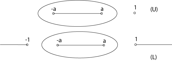
Figure 1: For a polynomial potential, including the ordinary Kazakov potential, the cut in the complex $z$-plane is $[-a,a]$ and $a_{c}=1$ (by normalization) as illustrated on the upper figure (U). The contour can be anywhere outside the cut, and in particularly we can choose it to also include $\pm a_{c}$. For the generalized Kazakov the contour is pinched between $[a,a_{c}]$ and $[-a_{c},-a]$ as shown on the lower figure (L). These intervals shrink to points for $g\to g_{*}$.

In the large $N$ limit we found the disk amplitude

$$gw_{0}(z)-\frac{1}{2}\tilde{V}_{s}^{\prime}(z)=-\frac{1}{2}\;\;{}_{2}F_{1}\!\Big{(}1,\frac{3}{2}\!-\!s,\frac{3}{2},\frac{z^{2}\!-\!a^{2}}{1\!-\!a^{2}}\Big{)}(1\!-\!a^{2})^{s-\frac{3}{2}}\sqrt{z^{2}\!-\!a^{2}}$$ (58)

where the relation between $a$ and $g$ is given by (55), i.e.

$$a^{2}=1-\left(1\!-\!g/g_{*}\right)^{1/(s-1/2)},\quad g_{*}=\frac{1}{4(s\!-\!1/2)}.$$ (59)

It is seen that the analytic structure of $gw_{0}(z)\!-\!\frac{1}{2}\tilde{V}_{s}(z)$ is very similar to the one given by (12), except that the function $M(z)$ is not a polynomial but an infinite power series. It allows us directly to take the scaling limit (15) and we obtain

$$gw_{0}(z)-\frac{1}{2}\tilde{V}^{\prime}_{s}(z)=-\frac{1}{2}\epsilon^{s-1}\left[(\sqrt{\Lambda})^{s-\frac{3}{2}}{}_{2}F_{1}\Big{(}1,\frac{3}{2}\!-\!s,\frac{3}{2};\frac{Z\!+\!\sqrt{\Lambda}}{\sqrt{\Lambda}}\Big{)}\right]\;\sqrt{Z\!+\!\sqrt{\Lambda}}.$$ (60)

The hypergeometric function has a power expansion in $Z\!+\!\sqrt{\Lambda}$ and it is seen that this is precisely the expansion in (16) with $\mu_{k}$ given in (65) below. In order to connect it to $W_{0}(Z)$ and $V^{\prime}_{cnt}(Z)$ in (16) we perform a Kummer transformation of the hypergeometric function and obtain

$$gw_{0}(z)-\frac{1}{2}\tilde{V}^{\prime}_{s}(z)=$$

$$-\epsilon^{s-1}\left((\sqrt{\Lambda})^{s-\frac{1}{2}}\;\frac{\sqrt{Z\!+\!\sqrt{\Lambda}}}{4(s-\frac{1}{2})Z}\;{}_{2}F_{1}\Big{(}1,s,\frac{1}{2}\!+\!s;-\frac{\sqrt{\Lambda}}{Z}\Big{)}+\frac{\sqrt{\pi}\Gamma(s\!-\!\frac{1}{2})}{4\Gamma(s)}\;(-Z)^{s-\frac{3}{2}}\sqrt{Z}\right).$$

From this we conclude that

$$W_{0}(Z)=\frac{(\sqrt{\Lambda})^{s-\frac{1}{2}}}{2}\;\left(-\frac{\sqrt{Z\!+\!\sqrt{\Lambda}}}{Z}\;{}_{2}F_{1}\Big{(}1,s,\frac{1}{2}\!+\!s;-\frac{\sqrt{\Lambda}}{Z}\Big{)}+\frac{1}{\sqrt{Z}}\right)$$ (62)

since this is the part which has an expansion in $Z^{-n-\frac{1}{2}}$, $n>0$. The rest is now identified with $V^{\prime}_{cnt}(Z)$:

$$V^{\prime}_{cnt}(Z)=\frac{(\sqrt{\Lambda})^{s-\frac{1}{2}}}{\sqrt{Z}}-\frac{\sqrt{\pi}\Gamma(s\!+\!\frac{1}{2})}{\Gamma(s)}\;\frac{(-Z)^{s-\frac{1}{2}}}{\sqrt{Z}},$$ (63)

i.e. we can write (making a somewhat arbitrary choice of how to divide $V^{\prime}_{cnt}(Z)$ into $\widetilde{T}_{s-\frac{1}{2}}$ and a $Z$ part for $s\!-\!\frac{1}{2}$ not an integer, the ambiguity caused by the cut along the positive real axis)

$$\frac{1}{2}T_{0}=\frac{1}{2}\widetilde{T}_{0}=(\sqrt{\Lambda})^{s-\frac{1}{2}},\qquad s\,\widetilde{T}_{s-\frac{1}{2}}=-\frac{\sqrt{\pi}\Gamma(s\!+\!\frac{1}{2})}{\Gamma(s)}.$$ (64)

It is seen by comparing with (17) that the potential in (63) does not have an expansion in powers $Z^{k+\frac{1}{2}}$. Let us try to understand why this is so, and how one can reach ordinary $T_{k}$’s as in the expansion (17).

Like the ordinary Kazakov potential, the so-called generalized Kazakov potential (56) only contains one adjustable coupling constant $g$, and the position of the cut of $w_{0}(z)$ is determined by (59). The difference is that the derivative of the potential has cuts along the real axis for $|z|>1$. This implies two things. Firstly we can still define the moments $M_{k}$ like in (10). We just have to choose the contour such that it encloses the cut $[-a,a]$ and avoids the cuts $|z|>1$ along the real axis. Once we make a deformation $t_{n}\to t_{n}\!+\!\delta t_{n}$ which leads to a scaling (14), the positions of the two cuts will change, but as long as they stay separated (which we will assume and examples of which we will provide below) we will have no problem with the choice of contour. This implies that almost all statements made when discussing the $m^{{\rm th}}$ multicritical matrix model in Sec. (2) which relate to the $\mu_{i}$ will still be valued. In particular (31) will remain valid. The “only” difference is that we now have infinitely many moments different from zero when we approach the critical point and that the higher moments become singular in the scaling limit.

This is true even for the plain generalized Kazakov model where we only have one coupling constant to adjust. In that case we have explicitly

$$M_{k}=d^{(s)}_{k}(1\!-\!a^{2})^{s-\frac{1}{2}-k}=\mu_{k}\epsilon^{s-\frac{1}{2}-k},\quad\mu_{k}=d^{(s)}_{k}(\sqrt{\Lambda})^{s-\frac{1}{2}-k},\quad k>0,$$ (65)

where

$$d^{(s)}_{k}=(-1)^{k-1}\;\frac{(s\!-\!\frac{1}{2})\cdots(s\!-\!(k\!-\!\frac{1}{2}))}{\frac{1}{2}\cdots(k\!-\!\frac{1}{2})}=-\frac{\Gamma(k\!+\!\frac{1}{2}\!-\!s)\Gamma(\frac{1}{2})}{\Gamma(\frac{1}{2}\!-\!s)\Gamma(k\!+\!\frac{1}{2})}.$$ (66)

Despite the increasing singular behavior of $M_{k}$ with increasing $k$, this behavior does not appear in (31). However, for $s\!-\!\frac{1}{2}$ non-integer the $T_{k}$’s defined by (24) are

$$\frac{1}{2}T_{0}=(\sqrt{\Lambda})^{s-\frac{1}{2}},\quad T_{k}=0,~{}~{}0<k<s-\frac{1}{2},\quad T_{k}=\infty~{}~{}k>s-\frac{1}{2}.$$ (67)

This singular behavior of the $T_{k}$’s is also seen in (25) where $T_{l}$ is divergent for $l>s-\frac{1}{2}$ provided $t_{2k}\propto 1/k^{s+1}$ for large $k$. This asymptotic behavior of the $t_{2k}$ results in a singular behavior of $xV^{\prime}(x)\sim(1\!-\!x^{2})^{s-1}$ and from the representation (19), using the last expression in eq. (10) for $M_{k}(t;a)$, it is indeed seen that such a behavior implies that $\tilde{M}_{k}$ becomes infinite for $k>s\!-\!\frac{1}{2}$.

This problem reflects that for a potential with the singularity structure like that of the generalized Kazakov potential (56) we cannot without qualifications use the definitions (19) and (22) for $\tilde{M}_{k}$ and $T_{k}$. The reason is that the contour integral in (19) had to encircle the cut $[-1,1]$, but the Kazakov potential has a cut on the positive real axis, starting from $z=1$. Stated differently, in order for (17) to make sense there has to be a region in the complex plane such that $(W_{0}(Z)-\frac{1}{2}V^{\prime}_{cnt}(Z))/\sqrt{Z}$ has a Laurent expansion. For a standard polynomial potential $V(z)$ the neighborhood of infinity always allows such an expansion. In the case of the generalized Kazakov potential there is no such region as is clear from the expressions (3)-(63). We can solve this problem by considering deformations $t_{n}\to t_{n}\!+\!\delta t_{n}$ which still have $a_{c}\!=\!1$ but where the cut of $V^{\prime}(z)$ approach $z\!=\!1$ from above when $\delta t_{n}\to 0$. Then we can define the $\tilde{M}_{k}$ and $T_{k}$ and everything stated with respect to the KdV-times $T_{k}$ will remain valid. To be explicit we will consider a class of deformations which are general enough to allow for an arbitrary finite number of independent KdV-times $T_{k}$ different from zero.

Let us start with the $t_{n}$’s corresponding to the generalized Kazakov potential (56). In this case we have one coupling constant which can be adjusted, $g$. We now introduce another adjustable parameter $\eta$ by making the deformation

$$t_{n}\to t_{n}\eta^{2n}=t_{n}+\delta t_{n},\quad\eta^{2}=1-\epsilon\nu<1,\quad{\rm i.e.}\quad V_{K}(z)\to V_{K}(\eta z),$$ (68)

which has a cut starting at $z=1/\eta\approx 1\!+\!\frac{1}{2}\epsilon\nu$. Following (65) we now have moments

$$M_{k}=d^{(s)}_{k}\eta^{2k}(1\!-\!\eta^{2}a^{2})^{s-\frac{1}{2}-k},\quad\mu_{k}=d^{(s)}_{k}(\sqrt{\Lambda}\!+\!\nu)^{s-\frac{1}{2}-k},\quad k>0,$$ (69)

and we obtain from (19) in analogy with (65)

$$\tilde{M}_{k}=d^{(s)}_{k}(1\!-\!\eta^{2})^{s-\frac{1}{2}-k},\quad{\rm i.e.}\quad(k\!+\!\frac{1}{2})T_{k}=d^{(s)}_{k}\nu^{s-\frac{1}{2}-k},\quad k>0.$$ (70)

For $k=0$ we have

$$M_{0}=\frac{g_{*}}{g}\big{(}1-\epsilon^{s-\frac{1}{2}}(\sqrt{\Lambda}\!+\!\nu)^{s-\frac{1}{2}}\big{)}\qquad\tilde{M}_{0}=\frac{g_{*}}{g}\big{(}1-\epsilon^{s-\frac{1}{2}}\nu^{s-\frac{1}{2}}\big{)},$$ (71)

which tell us (since $M_{0}=1$) that

$$\frac{g_{*}}{g}=1+\epsilon^{s-\frac{1}{2}}(\sqrt{\Lambda}\!+\!\nu)^{s-\frac{1}{2}},\qquad\frac{1}{2}T_{0}=(\sqrt{\Lambda}\!+\!\nu)^{s-\frac{1}{2}}-\nu^{s-\frac{1}{2}}.$$ (72)

The relation between $\mu_{k}$ and $T_{k}$ is given by (23), but while the summation in (23) is finite for a polynomial potential, it will not terminate in the present case. Again to be explicit, the corresponding continuum potential is

$$V^{\prime}_{cnt}(Z,\nu)=\sum_{n=0}^{\infty}(n\!+\!\frac{1}{2})T_{n}Z^{n-\frac{1}{2}}=\frac{(\sqrt{\Lambda}\!+\!\nu)^{s-\frac{1}{2}}}{\sqrt{Z}}-\frac{\nu^{s-\frac{1}{2}}}{\sqrt{Z}}\;{}_{2}F_{1}\Big{(}1,\frac{1}{2}\!-\!s,\frac{1}{2},\frac{Z}{\nu}\Big{)}$$ (73)

and $V^{\prime}_{cnt}(Z,\nu)\,\sqrt{Z}$ has a convergent power series for $|Z|<\nu$. Furthermore

$$W_{0}(Z)-\frac{1}{2}V^{\prime}_{cnt}(Z,\nu)=-(s\!-\!\frac{1}{2})\;\;{}_{2}F_{1}\Big{(}1,\frac{3}{2}\!-\!s,\frac{3}{2},\frac{Z\!+\!\sqrt{\Lambda}}{\nu\!+\!\sqrt{\Lambda}}\Big{)}\big{(}\nu\!+\!\sqrt{\Lambda}\big{)}^{s-\frac{3}{2}}\sqrt{Z\!+\!\sqrt{\Lambda}},$$ (74)

and for $\sqrt{\Lambda}<|Z|<\nu$ there is a convergent Laurent expansion of $(W_{0}(Z)\!-\!\frac{1}{2}V^{\prime}_{cnt}(Z,\nu))/\sqrt{Z}$ (see Fig. 2). By a suitable Kummer transformation one can show that $W_{0}(Z)/\sqrt{Z}$ for sufficient large $Z$ has a convergent expansion in $1/Z$, starting with the power $1/Z^{2}$.

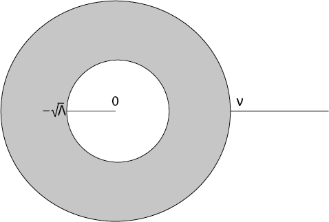
Figure 2: The annulus where $(W_{0}(Z)\!-\!\frac{1}{2}V^{\prime}_{cnt}(Z,\nu))/\sqrt{Z}$ has a Laurent expansion. The right cut is from $V^{\prime}_{cnt}(Z,\nu)/\sqrt{Z}$ given by (73) and starts at $\nu$, while the cut from 0 to $-\sqrt{\Lambda}$ is from $\sqrt{Z+\sqrt{\Lambda}}/\sqrt{Z}$.

It is now clear that we can obtain an arbitrary (finite) number of independent $\mu_{k}$ and $T_{k}$ by choosing a potential

$$V(z)=\sum_{a=1}^{L}c_{a}V_{K}(\eta_{a}z),\quad(k\!+\!\frac{1}{2})\;T_{k}=\sum_{a=1}^{L}c_{a}d_{k}^{(s)}\,\nu_{a}^{s-\frac{1}{2}-k},\quad\sum_{a=1}^{L}c_{a}=1,$$ (75)

and in this way we obtain a KdV hierarchy expressed in terms of the standard KdV times $T_{k}$. However, in general an infinite number of $T_{k}$ will be different from zero (but not independent of the $T_{k}$ with lower values of $k$). This implies that contrary to the situation for ordinary matrix models approaching a multicritical point of order $m$ the string equation (39) is now an infinite order differential equation in $T_{0}$ for the determination of $u$ and in this sense only practical useful when viewed as a genus expansion, in which case only a finite number of derivatives appear to each order. While the representation of perturbations around the generalized Kazakov potential is somewhat singular in terms of the standard KdV times $T_{k}$, it should be noted, and this will be used below, that the time $T_{0}$ is alway well defined and non-singular and the same is true for the function $u(T)$ and the representation in terms of Gelfand-Dikii polynomials $R_{n}(u)$.

4 The string equation

As seen above, contrary to the $\mu_{k}$, the standard KdV times $T_{k}$ are maybe not the most natural variables when we consider deformations away from the generalized Kazakov potential. This is not surprising. Recall that for the $m^{{\rm th}}$ multicritical Kazakov potential the anchor point was really $T_{m}\neq 0$ (and the rest of the $T_{k}$ equal zero, $k>0$). For the generalized Kazakov we had $T_{k}=0$ for $0<k<s-\frac{1}{2}$ and $T_{k}=\infty$ for $k>s-\frac{1}{2}$). What naturally replaced $T_{m}\neq 0$ was $\widetilde{T}_{s-\frac{1}{2}}\neq 0$ as seen in (63).

In the $m^{{\rm th}}$ Kazakov model deformations away from the pure model resulted in $T_{k}$ different from zero for $k=1,\ldots,m-1$ and these deformations could be viewed in a Wilsonian renormalization language as relevant deformations away from the multicritical point. Like in a renormalization group flow the “bare coupling constants”, the $\tilde{M}_{k}$, have to be turned to zero (like $\epsilon^{m-k}$). If $\tilde{M}_{k}$ is not tuned to zero the system will “flow” away from the neighborhood of the $m^{{\rm th}}$ multicritical point and to the $k^{{\rm th}}$ multicritical point when the “cutoff” $\epsilon$ is taken to zero, the lowest $k>0$ where $\tilde{M}_{k}\neq 0$ dominating. From this perspective, given a $m^{{\rm th}}$ multicritical point, the $T_{k}$, $k>m$ correspond to the (infinite) set of irrelevant deformations which naturally scale to zero when we approach the critical point (formerly $T_{k}=\epsilon^{k-m}\tilde{M}_{k}$, $\tilde{M}_{k}$ finite). Clearly the $T_{k}$ we have introduced above by deforming the potential away from the generalized Kazakov critical point corresponding to an index $s\neq m\!+\!\frac{1}{2}$ are slightly different in nature since we have infinite many of them, so the concept of relevant and irrelevant deformations does not apply in the same way. Maybe this is not surprising since the deformations of the $m^{{\rm th}}$ multicritical point and the $T_{k}$ have an interpretation in Liouville quantum gravity where they can be related to deformations corresponding to the $m$ (gravity dressed) primary operators in the $(2,2m\!-\!1)$ conformal field theory coupled to quantum gravity. However, for $s$ not a half-integer and in general an irrational number, the corresponding conformal field theory will in general be irrational and there is no obvious finite set of primary operators which can be considered as the relevant deformations. Thus a more natural starting point might be to consider a given generalized Kazakov potential $V_{s}(x)$ corresponding to an $s\neq m\!+\!\frac{1}{2}$ and then consider “relevant” deformations

$$V(x)=\sum_{0\leq k<s-\frac{1}{2}}\tilde{t}_{s-k}V_{s-k}(x),\quad\tilde{t}_{s-k}=O(\epsilon^{k}).$$ (76)

Such a potential will result in a continuum potential where

$$V^{\prime}_{cnt}(Z)=\sum_{0\leq k<s-\frac{1}{2}}(s-k)\widetilde{T}_{s-\frac{1}{2}-k}(-Z)^{s-\frac{1}{2}-k}/\sqrt{Z}$$ (77)

and as mentioned it would be the “naive” generalization of the relevant deformations around the Kazakov potential.

One can view it has a formal decomposition of any polynomial $V(x)$, changing coupling constants from $t_{k}$ to coupling constants $\tilde{t}_{s}$ in the same way as we could formally change from $t_{k}$ to $\epsilon^{m-k}T_{k}$ via formula (25). A priori it is not clear why a decomposition like (76) and correspondingly (77) should be chosen for an $s$ where $s-\frac{1}{2}$ is not an integer. It appears just to be an imitation of the situation for $s-\frac{1}{2}=m$, where there are good reasons for such an expansion, as explained above. Why not integrate over some range of $s$ since $s$ is a continuous variable rather than the discrete $m$? We can obtain some evidence in favor of the choice (77) by looking at the deformed potential (73). By a Kummer transformation the large $Z$ behavior of the potential is

$$V^{\prime}_{cnt}(Z,\nu)=-\frac{\sqrt{\pi}\Gamma(s\!+\!\frac{1}{2})}{\Gamma(s)}\;\frac{(-Z)^{s-\frac{1}{2}}}{\sqrt{Z}}\Big{(}1\!-\!\frac{\nu}{Z}\Big{)}^{s-1}+0(Z^{-\frac{1}{2}}).$$ (79)

Thus the potential $V^{\prime}_{cnt}(Z,\nu)$ indeed has a expansion like (77) in terms of potentials (63) with $s,s\!-\!1,\ldots$.

Let us now study in more detail the genus expansion associated with the simplest potential (63), the generalized Kazakov potential $V_{s}(x)$. The results can easily be extended to the more general potential (77). As mentioned above, formulated perturbatively and in terms of the moments $\mu_{k}$, everything is as for ordinary matrix models, except that we have infinitely many $\mu_{k}$ different from zero and explicitly given by (65). We thus have a well defined genus expansion. In fact, since we know all $\mu_{k}$ for the generalized Kazakov potential (see (65)) we can just insert them in the standard expression for the genus expansion, e.g. following [14].

There is however another way to obtain the genus expansion i.e. for the disk amplitude with one puncture with respect to $T_{0}$, $R(Z,u(T))$, namely first to solve the string equation for $u(T)$ and then to use (37) and (43). For the $m$’th multicritical model we have

$$\frac{1}{2}T_{0}=(\sqrt{\Lambda})^{m},\qquad(m\!+\!\frac{1}{2})T_{m}=\frac{(-1)^{m-1}\Gamma(\frac{1}{2})\Gamma(m\!+\!1)}{\Gamma(m+\frac{1}{2})},$$ (80)

and the contour in the string equation (36) can be deformed to infinity to give (39), which in the present case reads

$$(m\!+\!\frac{1}{2})T_{m}R_{m}(u)+\frac{1}{2}T_{0}R_{0}=0,\qquad\frac{1}{2}T_{0}=(\sqrt{\Lambda})^{m}.$$ (81)

In principle we can solve this finite order non-linear differential equation for $u$ and the solution has the form

$$u(T_{0},G)=-\sqrt{\Lambda}+\sum_{h=1}^{\infty}c_{h}\Big{(}\frac{G^{2}}{\Lambda^{m}}\Big{)}^{h}=-\Big{(}\frac{T_{0}}{2}\Big{)}^{\frac{1}{m}}+\sum_{h=1}^{\infty}c_{h}\Big{(}\frac{4G^{2}}{T_{0}^{2}}\Big{)}^{h}.$$ (82)

If we only are interested in the perturbative genus expansion in powers of $G^{2}$ equation (81) allows for a simple iterative algebraic determination of the coefficients $c_{h}$.

For the generalized Kazakov potential we have $\frac{1}{2}T_{0}=(\sqrt{\Lambda})^{s-\frac{1}{2}}$ but no longer a finite order differential equation which determines $u(T_{0},G)$. However we still have a simple algebraic procedure to determine the genus expansion of $u(T_{0},G)$. In this expansion the equivalent of (82) reads:

$$u(T_{0},G)=-\sqrt{\Lambda}+\sum_{h=1}^{\infty}c_{h}\Big{(}\frac{G^{2}}{\Lambda^{s-\frac{1}{2}}}\Big{)}^{h}=-\Big{(}\frac{T_{0}}{2}\Big{)}^{\frac{1}{s-\frac{1}{2}}}+\sum_{h=1}^{\infty}c_{h}\Big{(}\frac{4G^{2}}{T_{0}^{2}}\Big{)}^{h}.$$ (83)

The string equation (36) is still valid for the generalized Kazakov potential. We can think of the string equation as derived from the $\nu$ deformed potential (73) in the limit $\nu\to 0$. If we start with a situation where $\nu>\sqrt{\Lambda}$ we have a standard Laurent expansion, as explained above. Since we know the $T_{k}$ (eq. (70)), we can immediately write

$$\sum_{k=1}^{\infty}d^{(s)}_{k}\nu^{s-k-\frac{1}{2}}R_{k}(u)+\frac{1}{2}T_{0}R_{0}=0,\qquad\frac{1}{2}T_{0}=(\sqrt{\Lambda}+\nu)^{s-\frac{1}{2}}-\nu^{s-\frac{1}{2}}.$$ (84)

This infinite order differential equation looks singular for $\nu\to 0$. However, using

$$R_{k}(u)=\sum_{l=0}^{k}c^{(l)}_{k-l}(-u)^{k-l}\tilde{R}_{l}(u),\qquad c^{(l)}_{k-l}d^{(s)}_{k}=c^{(l-s)}_{k-l}d^{(s)}_{l},$$ (85)

where the first equation is the inverse of the equation in (45) and where $c^{(k)}_{n}$ and $d^{(s)}_{k}$ are defined by (23) and (65), we obtain (for $\nu>|u|$)

$$\sum_{k=0}^{\infty}d^{(s)}_{k}(\nu-u)^{s-\frac{1}{2}-k}\tilde{R}_{k}(u)+\frac{1}{2}(\sqrt{\Lambda}+\nu)^{s-\frac{1}{2}}=0.$$ (86)

This equation is regular in the limit $\nu\to 0$ and the final string equation is thus

$$\sum_{k=0}^{\infty}d^{(s)}_{k}(-u)^{s-\frac{1}{2}-k}\tilde{R}_{k}(u)+\frac{1}{2}T_{0}\tilde{R}_{0}=0,\qquad\frac{1}{2}T_{0}=(\sqrt{\Lambda})^{s-\frac{1}{2}},$$ (87)

and for genus 0 it gives precisely $-(-u)^{s-\frac{1}{2}}+\frac{1}{2}T_{0}=0$, i.e. $u=-\sqrt{\Lambda}$.

The string equation could have been derived simpler starting from the expansion (45). Again taking $\nu>0$ the contour $C_{1}$ exists and will enclose the cut $[u,0]$ and one obtains

$$\lim_{\nu\to 0}\oint_{C_{1}}\frac{d\Omega}{2\pi i}\;V^{\prime}_{cnt}(\Omega,\nu)\;\frac{\tilde{R}_{k}(u)}{(\Omega\!-\!u)^{k+\frac{1}{2}}}=d_{k}^{(s)}(-u)^{s-\frac{1}{2}-k}\tilde{R}_{k}(u),\quad k>0,$$ (88)

while the integral for $k=0$ is $\frac{1}{2}\big{(}(\sqrt{\Lambda})^{s-\frac{1}{2}}\!-\!(-u)^{s-\frac{1}{2}}\big{)}$. The result is obtained either by contracting the integral to the cut or deforming it to infinity (details are provided in the Appendix). The string equation follows immediately and in this derivation we do not have to assume $\nu>|u|$ as a starting point.

As mentioned, in general the string equation (87) will be an infinite order differential equation. Since $d^{(s)}_{k}\!=\!0$ for $s\!-\!\frac{1}{2}=m$ and $k>m$ the infinite series in (87) will in this case terminate we recover the string equation (81) for the $m$’th multicritical matrix model. However, viewed as a genus expansion of $u$ in powers of $G^{2}$ eq. (87) is not much different from the “ordinary” string equation. As mentioned already below eq. (51), if we want to solve (87) up to order $h$, using the expansion (52), it will involve only the first $3h$ terms in (87) and to obtain these we only have to solve iteratively eq. (48) up to order $h$. Using (49)-(51) the string equation (87) to order $G^{4}$ reads:

$$\frac{1}{4}T_{0}=(-u)^{s-1/2}\frac{1}{2}+G^{2}(-u)^{s-5/2}\;\frac{2^{2}(s\!-\!\frac{1}{2})(s\!-\!\frac{3}{2})}{1\cdot 3}\left[\frac{u^{(2)}}{4}+\frac{2(s\!-\!\frac{5}{2})}{5\cdot u}\frac{(u^{\prime})^{2}}{16}\right]$$ (89)

$$+G^{4}(-u)^{s-\frac{7}{2}}\;\frac{2^{3}(s\!-\!\frac{1}{2})(s\!-\!\frac{3}{2})(s\!-\!\frac{5}{2})}{1\cdot 3\cdot 5}\left[\frac{u^{(4)}}{4}+\frac{2(s-\frac{7}{2})}{7\cdot u}\Big{(}\frac{28u^{\prime}u^{(3)}\!+\!21(u^{(2)})^{2}}{16}\Big{)}\right.$$

$$+\frac{2^{2}(s\!-\!\frac{7}{2})(s\!-\!\frac{9}{2})}{7\cdot 9\cdot u^{2}}\Big{(}\frac{231}{32}(u^{\prime})^{2}u^{(2)}\Big{)}\left.+\frac{2^{3}(s\!-\!\frac{7}{2})(s\!-\!\frac{9}{2})(s\!-\!\frac{11}{2})}{7\cdot 9\cdot 11\cdot u^{3}}\frac{1155}{256}(u^{\prime})^{4}\right]$$

which allows us to determine the coefficients $c_{h}$ in eq. (83) for the expansion of $u$ in powers of $G^{2}$.

5 Discussion

We have studied perturbations around and the genus expansion of the generalized Kazakov model we introduced in [11]. The model serves as a prototype for matrix models where the coefficients in potential $V(x)=\sum_{n}t_{n}x^{n}$ behave as $t_{n}\sim 1/n^{s+1}$ for $n\to\infty$. When the pertubation away from the Kazakov potential $V_{s}(x)$ was formulated in terms of the so-called moments $M_{k}$ and $\mu_{k}$, everything was a simple generalization of what happens for polynomial potentials, except for the the fact that we have infinitely many moments $M_{k}$ and $\mu_{k}$ different from zero, contrary to the polynomial case where perturbations around the $m^{{\rm th}}$ multicritial point only involve moments $\mu_{1},\ldots,\mu_{m}$ in the scaling limit. Despite the fact that the moments $M_{k}$ become increasingly singular in the scaling limit for $k>s\!-\!\frac{1}{2}$, the standard formulas for polynomial potentials valid for any polynomial interactions as well as to any order in the genus expansion are still valid. The increasingly singular behavior of the moments $M_{k}$ cancel in the expressions for multiloop correlations leaving us with finite expressions for the multiloop correlators when expressed in terms of the scaled moments $\mu_{k}$. These expressions are identical to the expression for a standard multicritical matrix model with a sufficiently high $m$ (recall that for a given multiloop function and expanded to a given order, only a finite number of $\mu_{k}$ will appear).

However, the situation was less clear when it came to the relation to the KdV-structure of ordinary, polynomial one-matrix models. The problem is that the continuum potential in the case of the generalized Kazakov model does not have an asymptotic expansion $\sum_{n}T_{n}Z^{n+\frac{1}{2}}$ which allows us to define the continuum coupling constants $T_{k}$ which serve as KdV-times in the KdV hierarchy equations. We have shown that by a suitable deformation away from the pure generalized Kazakov model one can indeed define such times. One important difference to the standard KdV situation is however that at least for the class of deformations we consider, one always has an infinite set of $T_{k}$ which are not independent. We showed that one can make an arbitrary finite set of these $T_{k}$ independent, but a basic property of the KdV hierarchy, namely that it forms a closed system of differential equations for any finite set of $T_{k}$ is not true for our system. We will have a system of differential equations of infinite order where one can choose arbitrarily a finite set of independent $T_{k}$, but this is somewhat different from being able to choose a finite set of $T_{k}$. Assuming that there still is an integrable structure behind these equations, this suggests one should be able to choose a different set of times $\widetilde{T}_{k}$ by extracting the singularity in the series expansion of the continuum potential $\sum_{n}\widetilde{T}_{n}Z^{n+\alpha}$ with $\alpha=s\!-\![s]$, where the standard KdV properties are satisfied. We suggested such a set, but it is not yet clear if they can serve as genuine KdV times.

Finally we addressed the question of the genus expansion of $R(Z,u)$ for the generalized Kazakov model. As mentioned above the genus expansion is unproblematic when formulated in terms of the moments $\mu_{k}$. However, the genus formulation for $R(Z,u)$ is usually nicely formulated via the string equation which (in principle) can be solved for $u(T)$ to all orders in the genus expansion, after which one can find the genus expansion of $R(Z,u)$. Since the string equation in terms of the $T_{k}$ is not available for us for the generalized Kazakov model (no $T_{k}$, $k>0$), we investigated in detail the string equation for the generalized Kazakov model and showed how the string equation still led to a perturbative determination of the function $u(T_{0})$ via an equation which reduced to the standard finite order differential equation for $s\!-\!\frac{1}{2}=m$. We also showed that the string equation is nicely formulated via the times $\widetilde{T}_{k}$ when $s$ is not half-integer.

Acknowledgments

We are grateful to Timothy Budd for useful discussions at early stages of this work. The authors acknowledge the support by the ERC Advanced grant 291092, “Exploring the Quantum Universe” (EQU) as well as the Dainish Research Council grant “Quantum Geometry”. L. C. and Y. M.  thank the Theoretical Particle Physics and Cosmology group at the Niels Bohr Institute for the hospitality.

Appendix

Let $\nu>0$. Thus the deformed potential $V^{\prime}_{cnt}(Z,\nu)$ is analytic in the region $Z\in]0,\nu[$ and the contour integral

$$I_{k}(u,\nu):=\oint_{C_{1}}\frac{d\Omega}{2\pi i}\;\frac{V^{\prime}_{cnt}(\Omega,\nu)}{(\Omega\!-\!u)^{k+\frac{1}{2}}}=\frac{1}{\Gamma(k\!+\!\frac{1}{2})}\frac{d^{k}I_{0}(u,\nu)}{du^{k}}$$ (90)

around $C_{1}$ is well defined and can be calculated by contracting the contour to the cut $[u,0]$. Once this is done there is no problem taking $\nu\to 0$ and we end up with the integral

$$\int^{0}_{u}\frac{dx}{\pi}\;\left(\frac{(\sqrt{\Lambda})^{s-\frac{1}{2}}}{\sqrt{-x}}-\frac{\sqrt{\pi}\Gamma(s+\frac{1}{2})}{\Gamma(s)}\;\frac{(-x)^{s-\frac{1}{2}}}{\sqrt{-x}}\right)\;\frac{1}{\sqrt{-u-x}}=(\sqrt{\Lambda})^{s-\frac{1}{2}}-(-u)^{s-\frac{1}{2}}.$$ (91)

We thus have

$$I_{0}(u,0)=(\sqrt{\Lambda})^{s-\frac{1}{2}}-(-u)^{s-\frac{1}{2}},\qquad I_{k}(u,0)=d^{(s)}_{k}(-u)^{s-\frac{1}{2}-k}.$$ (92)

If we instead deform the contour to infinity and along the cut of $V^{\prime}_{cnt}(Z,\nu)$ on the positive real axis starting at $\nu$ we can express the string equation in terms of the Mellin transform of $R(Z,u)$. Again, after the deformation we can take $\nu\to 0$ and we will assume this is done in the following. For $k>s\!-\!\frac{1}{2}$ the contribution to $I_{k}(u,0)$ from the contour at infinity will vanish and we have left with the contribution from the cut:

$$I_{k}(u,0)=\cos\pi s\int_{0}^{\infty}\frac{dx}{\pi}\frac{\sqrt{\pi}\Gamma(s+\frac{1}{2})}{\Gamma(s)}\frac{x^{s-1}}{(x\!-\!u)^{k+\frac{1}{2}}}.$$ (93)

For $k<s\!-\!\frac{1}{2}$ there is a contribution from the contour at infinity and this contribution exactly cancels the contribution from the integral in (93) for large $x$ since $I_{k}(u,0)$ of course is independent of the choice of contour. We can thus view (93) as valid for all $s$ provided we subtract from the integrand a sufficient number of terms of the Taylor expansion around infinity to ensure convergence of the integral at infinity. This is exactly what is done for Mellin transformations defined as follows

$$\tilde{f}(s):={\cal M}[f](s)=\int_{0}^{\infty}dx\;x^{s-1}f(x),\quad{\cal M}^{(-1)}[\tilde{f}](x)=\int_{\gamma-i\infty}^{\gamma+i\infty}ds\;x^{-s}\tilde{f}(s),$$ (94)

if the integral is divergent at infinity. We can thus write

$${\cal M}[(x-u)^{-k-\frac{1}{2}}](s)=(-u)^{s-\frac{1}{2}-k}d^{(s)}_{k}\;\frac{\Gamma(s)\Gamma(\frac{1}{2}\!-\!s)}{\Gamma(\frac{1}{2})},$$ (95)

and applying to $R(Z,u)$ we have

$${\cal M}[R(\cdot,u)](s):=\int_{0}^{\infty}dxx^{s-1}R(x,u)=\frac{\Gamma(s)\Gamma(\frac{1}{2}\!-\!s)}{\Gamma(\frac{1}{2})}\sum_{k=0}^{\infty}d^{(s)}_{k}(-u)^{s-\frac{1}{2}-k}\tilde{R}(u).$$ (96)

We can thus write the string equation as

$${\cal M}[R(\cdot,u)](s)=-T_{0}\frac{\Gamma(s)\Gamma(\frac{1}{2}\!-\!s)}{2\sqrt{\pi}},$$ (97)

where the term on the rhs comes from the $\frac{1}{2}T_{0}/\sqrt{Z}$ part of the potential $V^{\prime}_{cnt}(Z)$ in the string equation. This equation looks intriguing simple and one could be tempted to apply the inverse Mellin transform to find $R(x,u)$ since the inverse Mellin transform of the rhs is just where the $R_{0}(x,-\sqrt{\Lambda})$ given by (25). Unfortunately the subtlety of the equation is not in $x$ and $s$ but in $u(T_{0})$, since $R(x,u)$ is the generating function of the Gelfand-Dikii polynomials. If the double scaling parameter $G$ is equal to zero this becomes a triviality and one indeed finds $R(x,u)$ simply be an inverse Mellin transform of (97).

References

- [1] V. A. Kazakov, Mod. Phys. Lett. A 4 (1989) 2125.
- [2] M. Staudacher, Nucl. Phys. B 336 (1990) 349.
- [3] P. Di Francesco, P. Ginsparg and J. Zinn-Justin, Phys. Rept. 254 (1995) 1.
-
[4]
J. Ambjorn, B. Durhuus and J. Frohlich,
Nucl. Phys. B 257 (1985) 433;
Nucl. Phys. B 275, 161 (1986).
J. Ambjorn, B. Durhuus, J. Frohlich and P. Orland, Nucl. Phys. B 270, 457 (1986).
F. David, Nucl. Phys. B 257, 45 (1985); Nucl. Phys. B 257, 543 (1985).
A. Billoire and F. David, Nucl. Phys. B 275, 617 (1986).
V. A. Kazakov, Phys. Lett. B 150 (1985) 282.
V. A. Kazakov, A. A. Migdal and I. K. Kostov, Phys. Lett. B 157, 295 (1985).
D. V. Boulatov, V. A. Kazakov, I. K. Kostov and A. A. Migdal, Nucl. Phys. B 275, 641 (1986). -
[5]
J. Ambjorn, J. Jurkiewicz, Phys. Lett. B278 (1992) 42
M. E. Agishtein and A. A. Migdal, Mod. Phys. Lett. A 7 (1992) 1039; Nucl. Phys. B 385 (1992) 395. - [6] J. Ambjorn, A. Goerlich, J. Jurkiewicz and R. Loll, Phys. Rept. 519 (2012) 127, [arXiv:1203.3591,[ hep-th]].
-
[7]
J. Ambjorn, A. Görlich, J. Jurkiewicz and R. Loll,
Phys. Rev. Lett. 100 (2008) 091304 [arXiv:0712.2485 [hep-th]].
Phys. Rev. D 78 (2008) 063544 [arXiv:0807.4481 [hep-th]].
Phys. Lett. B 690 (2010) 420-426 [arXiv:1001.4581 [hep-th]].
J. Ambjorn, J. Jurkiewicz and R. Loll, Phys. Rev. Lett. 93 (2004) 131301 [hep-th/0404156]. Phys. Rev. D 72 (2005) 064014 [hep-th/0505154]. Phys. Lett. B 607 (2005) 205-213 [hep-th/0411152].
J. Ambjorn, A. Gorlich, S. Jordan, J. Jurkiewicz and R. Loll, Phys. Lett. B 690 (2010) 413 [arXiv:1002.3298, hep-th].
J. Ambjorn, S. Jordan, J. Jurkiewicz and R. Loll, Phys. Rev. Lett. 107 (2011) 211303 [arXiv:1108.3932 [hep-th]]. Phys. Rev. D 85 (2012) 124044 [arXiv:1205.1229 [hep-th]]. -
[8]
J. Ambjorn and Y. Watabiki,
Nucl. Phys. B 445 (1995) 129,
[hep-th/9501049];
J. Ambjorn, J. Jurkiewicz and Y. Watabiki, Nucl. Phys. B 454 (1995) 313, [hep-lat/9507014].
J. Ambjorn and K. Anagnostopoulos, Nucl. Phys. B 497 (1997) 445, [hep-lat/9701006].
J. Ambjorn, K. N. Anagnostopoulos, U. Magnea and G. Thorleifsson, Phys. Lett. B 388 (1996) 713, [hep-lat/9606012]. -
[9]
M. Fukuma, H. Kawai and R. Nakayama,
Int. J. Mod. Phys. A 6 (1991) 1385;
R. Dijkgraaf, H. Verlinde and E. Verlinde, Nucl. Phys. B 348 (1991) 435. - [10] A. Gerasimov, Y. Makeenko, A. Marshakov, A. Mironov, A. Morozov and A. Orlov, Mod. Phys. Lett. A 6 (1991) 3079.
- [11] J. Ambjorn, T. Budd and Y. Makeenko, Nucl. Phys. B 913 (2016) 357 [arXiv:1604.04522 [hep-th]].
- [12] J. Ambjorn and Y. Makeenko, Mod. Phys. Lett. A 5 (1990) 1753.
- [13] J. Ambjorn, J. Jurkiewicz and Y. Makeenko, Phys. Lett. B 251 (1990) 517.
- [14] J. Ambjorn, L. Chekhov, C. Kristjansen and Y. Makeenko, Nucl. Phys. B 404 (1993) 127; Erratum: Nucl. Phys. B 449 (1995) 681 [hep-th/9302014].
- [15] Y. Makeenko, A. Marshakov, A. Mironov and A. Morozov, Nucl. Phys. B 356 (1991) 574.
- [16] J. Ambjorn, B. Durhuus and T. Jonsson, Quantum geometry. A statistical field theory approach, Cambridge (UK) Univ. Press (1997).