Critical Wess-Zumino models with four supercharges from the functional renormalization group

Abstract

We analyze the $\mathcal{N}=1$ supersymmetric Wess-Zumino model dimensionally reduced to the $\mathcal{N}=2$ supersymmetric model in three Euclidean dimensions. As in the original model in four dimensions and the $\mathcal{N}=(2,2)$ model in two dimensions the superpotential is not renormalized. This property puts severe constraints on the non-trivial fixed-point solutions, which are studied in detail. We admit a field-dependent wave function renormalization that in a geometric language relates to a Kähler metric. The Kähler metric is not protected by supersymmetry and we calculate its explicit form at the fixed point. In addition we determine the exact quantum dimension of the chiral superfield and several critical exponents of interest, including the correction-to-scaling exponent $\omega$, within the functional renormalization group approach. We compare the results obtained at different levels of truncation, exploring also a momentum-dependent wave function renormalization. Finally we briefly describe a tower of multicritical models in continuous dimensions.

I Introduction

In the challenge of understanding strongly interacting quantum field theories, progress has often been associated to the special role played by symmetries. Among them, conformal symmetry and supersymmetry have been of particular relevance in recent developments in quantum field theory (QFT) and particle physics. This line of progress has been a perfect embodiment of the principle that understanding goes along with simplicity. Yet, complexity is ubiquitous and the development of general tools to address it is also an important field of research. Thus, bringing together powerful symmetries and general mathematical methods can be fruitful – the reliability of the latter can be tested against the exact constraints imposed by the former.

Remarkably, this kind of analysis is still missing in several simple arenas offered by QFT. Such is the $\mathcal{N}=1$ four-dimensional Wess-Zumino (WZ) model Wess and Zumino (1974), and its dimensional reduction to three dimensions, namely the $\mathcal{N}=2$ model in three dimensions. While the former has been a seminal example of four-dimensional supersymmetric field theory and heavily influenced particle phenomenology, the latter case and its further reduction to two dimensions have found surprising applications to statistical systems, mainly thanks to the phenomenon of universality.

Two dimensional minimal conformal models with $\mathcal{N}=(2,2)$ supersymmetry Fateev and Zamolodchikov (1985); Di Vecchia et al. (1986); Mussardo et al. (1989) have been related to two-dimensional self-dual critical points of $\mathbb{Z}_{N}$-symmetric statistical systems, and are benchmark examples of exactly solvable strongly interacting QFTs. The relation between these field theories and statistical models has even been extended away from criticality Cecotti and Vafa (1993a, b). Though these successes deeply rely on the infinite dimensional superconformal symmetry that is special of two dimensions, some of them are based on another remarkable property of these models, which is present also in absence of conformal symmetry and in higher dimensions: the nonrenormalization of the superpotential. This has been used, for instance, to obtain a generic classification of $\mathcal{N}=2$ superconformal models in two dimensions Vafa and Warner (1989), through the language of Landau-Ginzburg effective Lagrangians and their renormalization group (RG) flow. The latter has also been discussed in the framework of conformal perturbation theory in Ref. Bienkowska (1993).

The nonrenormalization of the superpotential has been discovered by means of perturbation theory in four dimensions Wess and Zumino (1974); Iliopoulos and Zumino (1974); Grisaru et al. (1979). Later on it has been further analyzed nonperturbatively by holomorphy arguments Seiberg (1993) and by algebraic methods Flume and Kraus (2000). These results refer to the four-dimensional $\mathcal{N}=1$ WZ model, which is expected to be trivial, i. e. incomplete, beyond pertubation theory. Yet, similar arguments can be used in less than four dimensions where such a problem is not present.

In fact, dimensional arguments suggest that non-trivial scale-invariant models with four supercharges should exist below four dimensions. Supporting evidence comes from comparison with the non-supersymmetric counterpart of this field theory, the bosonized Nambu$-$Jona-Lasinio model (the Gross-Neveu model with U$(1)$ chiral symmetry) which can be studied perturbatively by means of $\epsilon$ and $1/N_{f}$ expansions Rosenstein et al. (1991); Gracey (1993, 1994); Kleinert and Babaev (1998). The existence of a continuous phase transition in this model has also been confirmed by extensive Monte Carlo studies Karkkainen et al. (1994); Hands et al. (1993, 1995); Barbour et al. (1999); Hands et al. (2001); Christofi and Strouthos (2007); Chandrasekharan and Li (2013); Hesselmann and Wessel (2016). Under the assumption that the critical point survives in the $N_{f}\to 1/2$ limit, i. e. with one Majorana fermion in four dimensions or one Dirac fermion in three dimensions, the resulting critical field theory is expected to enjoy supersymmetry, thus representing a non-trivial $\mathcal{N}=2$ scale-invariant WZ model in three dimensions Strassler (2003). The possibility that this supersymmetric fixed point exists in three dimensions and the constraints on it stemming from the nonrenormalization of the superpotential have already been discussed through holomorphy in Ref. Aharony et al. (1997).

This three-dimensional critical QFT has received much attention recently, as a candidate for the emergence of supersymmetry in the long-distance physics of condensed matter systems Thomas (2005). Concerning such systems, several specific proposals were made Lee (2007, 2010); Ponte and Lee (2014); Grover et al. (2014). For dedicated QFT analyses of emergent supersymmetry see also Refs. Sonoda (2011); Fei et al. (2016); Zerf et al. (2016); Gies et al. (2017); Zhao and Liu (2017). These works brought constructive evidence about the existence of scale-invariant three-dimensional models with $\mathcal{N}=1$ and $\mathcal{N}=2$ supersymmetry, but for the $\mathcal{N}=2$ model only through a perturbative $\epsilon$ expansion about four dimensions. Since the non-trivial fixed point is at strong coupling in three dimensions, nonperturbative techniques are needed to investigate its properties. Among them, the conformal bootstrap has put bounds on several quantities of interest, supporting the conjecture that the fixed point exists between four and two dimensions and enjoys superconformal symmetry Bobev et al. (2015a, b). In addition, exact determinations of the sphere free energy Jafferis (2012) and of the coefficient $C_{T}$ entering the stress-tensor two-point function Imamura and Yokoyama (2012); Closset et al. (2013); Nishioka and Yonekura (2013) have been provided through localization.

Clearly, other studies with different tools would be helpful to get a more comprehensive picture of WZ models with four supercharges. This is the goal of the present work, where we adopt a nonperturbative functional renormalization group (FRG) method that can be applied to study strongly interacting QFTs in a continuous number of dimensions. The FRG has the virtue of including both perturbative and nonperturbative approximations in one analytic differential framework, which strongly resembles Schwinger-Dyson equations. Since its very birth Wilson and Kogut (1974); Wegner and Houghton (1973) this method has been extensively applied to critical phenomena, especially in three-dimensional Euclidean spacetime, both for spin-zero and spin-one-half field theories. Some illustrative examples and a thorough discussion of the method can be found in several reviews Berges et al. (2002); Kopietz et al. (2010); Gies (2012).

This framework has been shown to yield compelling results in three-dimensional critical Yukawa models at zero temperature and density Rosa et al. (2001); Hofling et al. (2002); Strack et al. (2010); Gies et al. (2010); Braun et al. (2011); Sonoda (2011); Scherer and Gies (2012); Janssen and Gies (2012); Janssen and Herbut (2014); Gehring et al. (2015); Vacca and Zambelli (2015); Classen et al. (2016, 2017). A relevant subclass of such systems – supersymmetric models – has also been under the focus of the FRG. Especially in three dimensions, the $\mathcal{N}=1$ WZ model has been studied in greater detail Synatschke et al. (2010); Heilmann et al. (2015); Hellwig et al. (2015); Gies et al. (2017), but also O(N) models have been addressed Heilmann et al. (2012). Concerning theories with four supercharges, applications have been essentially limited to reproducing the nonrenormalization of the superpotential in four Rosten (2010); Sonoda and Ulker (2010), three Osborn and Twigg (2012) and two dimensions, and to an analysis of the two-point function in the latter case Synatschke-Czerwonka et al. (2010).

In contrast, this work is devoted to the construction and characterization of non-trivial fixed points. As such, it is an exploratory study that lays the basis for a more comprehensive FRG analysis. In particular, in Sec. II we recall the definition of the four and three-dimensional models and the dimensional reduction that links them. In Sec. III we adopt the three-dimensional parametrization to detail the FRG framework. In Sec. IV we discuss the constraints that the nonrenormalization of the superpotential imposes on the fixed points of the RG in arbitrary dimensions, including the exact determination of the quantum dimension of the chiral superfield and several critical exponents, at an infinite tower of non-trivial scale-invariant models. In Sections V, VI and VII we analyze the three-dimensional non-trivial critical point, focusing on the correction-to-scaling exponent $\omega$ which is not constrained by supersymmetry, as a case study for probing the quality of perturbative and nonperturbative approximations within the FRG. Section V contains the simplest computation, that only accounts for the running of the wave function renormalization. Section VI includes the RG flow of a field-dependent Kähler metric, while Sec. VII, explores the effect of addressing the momentum dependence of the Kähler metric. The remaining infinite number of RG fixed points is addressed in Sec. VIII. Here we perform the minimal analysis to support their existence in continuous dimensions between three and two, and to show that they describe genuine non-Gaussian models; that is, we perform an $\epsilon$ expansion around the corresponding upper critical dimensions, within the truncation of a field-dependent Kähler metric. We conclude in Sec. IX with a summary of our results and an outlook. Subsidiary information is provided in the Appendix.

II The Wess-Zumino model in four and three dimensions

Our starting point is the WZ model

$$\begin{split}\mathcal{L}_{4}=&\;\partial_{\mu}\phi\partial^{\mu}\!\phi^{\dagger}+\frac{i}{2}\bar{\psi}\not{\partial}\psi+f\!f^{\dagger}\\ &+\left\{\frac{\partial W(\phi)}{\partial\phi}f-\frac{1}{4}\bar{\psi}(1-\Gamma_{5})\frac{\partial^{2}W(\phi)}{\partial\phi^{2}}\psi+\operatorname{h.\!c.}\right\}\end{split}$$ (1)

in four-dimensional Minkowski spacetime. $W$ denotes an arbitrary holomorphic superpotential of the form

$$W(\phi)=\sum\limits_{n=1}^{\infty}\frac{C_{n}}{n}\phi^{n}\,.$$ (2)

The fields $\phi$ and $f$ are complex scalars whereas $\psi$ is a Majorana spinor.

Dimensional reduction allows to “downscale” $\mathcal{L}_{4}$ to three Euclidean dimensions through compactification of the time direction. Technically, the time dependence of the fields is abandoned and their canonical dimensions are adjusted to ensure that a three-dimensional integration over (1) yields a dimensionless result. The obtained expression can be understood as a Lagrangian density in three dimensions.

To rewrite it in a familiar form it is useful to pick a particular representation of the four and three-dimensional Dirac matrices $\Gamma^{\mu}$ resp. $\gamma^{j}$:

$$\Gamma^{0}=\sigma^{2}\otimes\mathbb{1},\;\;\Gamma^{j}=\sigma^{3}\otimes\gamma^{j}$$ (3)

We choose the three-dimensional Dirac matrices proportional to the Pauli matrices, $\gamma^{j}=i\sigma^{j}$. The equality

$$[\Gamma^{i},\Gamma^{j}]=\mathbb{1}\otimes[\gamma^{i},\gamma^{j}]$$ (4)

ensures that

$$\psi=(1,0)^{T}\!\otimes\psi_{1}+(0,1)^{T}\!\otimes\psi_{2}$$ (5)

defines three-dimensional (two component) spinors $\psi_{1}$ and $\psi_{2}$.

Introducing the Dirac spinor

$$\tilde{\psi}=\frac{1}{\sqrt{2}}(\psi_{1}+\psi_{2})$$ (6)

and abandoning the tilde we end up with the three-dimensional, Euclidean $\mathcal{N}=2$ WZ model

$$\begin{split}\mathcal{L}_{3}=&\;\partial_{j}\phi\partial^{j}\!\phi^{\dagger}+i\bar{\psi}\sigma^{j}\partial_{j}\psi-f\!f^{\dagger}\\ &-\left\{W^{\prime}f-\frac{1}{2}W^{\prime\prime}\psi^{T}\sigma^{2}\psi+\operatorname{h.\!c.}\right\}.\end{split}$$ (7)

The Lagrangian density (7) is, up to a total derivative, invariant under the supersymmetry transformations

$$\begin{split}\delta_{\alpha}\phi&=\sqrt{2}\alpha^{T}\!\sigma^{2}\psi,\\ \delta_{\alpha}f&=i\sqrt{2}\bar{\alpha}\sigma^{j}\partial_{j}\psi,\\ \delta_{\alpha}\psi&=\sqrt{2}(f\alpha-i\sigma^{j}\partial_{j}\phi\sigma^{2}\!\alpha^{*}).\end{split}$$ (8)

The three-dimensional model 7 can be constructed from the chiral superfield

$$\begin{split}\Phi(x,\theta,\bar{\theta})=&\operatorname{e}^{\delta_{\theta}}\!\phi(x)\\ =&\operatorname{e}^{-i\bar{\theta}\sigma^{j}\theta\partial_{j}}(\phi+\sqrt{2}\theta^{T}\!\sigma^{2}\psi+\theta^{T}\!\sigma^{2}\theta f)\end{split}$$ (9)

with $\delta_{\theta}$ defined by (8). The Lagrangian density (7) is, up to a surface term, identical to

$$\begin{split}\mathcal{L}_{3}=&-\frac{1}{4}\int\!\operatorname{d}^{2}\!\theta\operatorname{d}^{2}\!\bar{\theta}\;\Phi\Phi^{\dagger}\\ &-\left\{\frac{1}{2i}\int\!\operatorname{d}^{2}\!\theta\;W(\Phi)+\operatorname{h.\!c.}\right\}.\end{split}$$ (10)

The super-covariant derivatives take the form

$$\begin{split}D&=i\sigma^{j}\theta\partial_{j}+\partial_{\bar{\theta}},\\ \bar{D}&=-i\bar{\theta}\sigma^{j}\partial_{j}-\partial_{\theta}.\end{split}$$ (11)

These derivatives allow us to write the most generic Lagrangian density of the $\mathcal{N}=2$ three-dimensional WZ model as Rosten (2010)

$$\begin{split}\mathcal{L}=&-\frac{1}{4}\int\!\operatorname{d}^{2}\!\theta\operatorname{d}^{2}\!\bar{\theta}\;\mathcal{K}(D,\bar{D},\Phi,\Phi^{\dagger})\\ &-\left\{\frac{1}{2i}\int\!\operatorname{d}^{2}\!\theta\;W+\operatorname{h.\!c.}\right\}\,,\end{split}$$ (12)

where $\mathcal{K}$ is an arbitrary real, scalar, analytic function of $\Phi$, $\Phi^{\dagger}$, and of the covariant derivatives, which act on the fields. Though $\mathcal{K}$ is sometimes called the Kähler potential, we reserve this designation for $K(\Phi,\Phi^{\dagger})$, containing only the $D$- and $\bar{D}$-independent contributions to the generalized Kähler potential $\mathcal{K}$. Throughout this paper we stick to real coupling constants $C_{n}$ in the expansion (2) of the superpotential, though this is not required by symmetry. Our conventions are summarized in App. A.

III The functional renormalization group

The modern implementation of the FRG is formulated in terms of one-particle-irreducible (1PI) correlation functions Wetterich (1993); Morris (1994a); Ellwanger (1994); Bonini et al. (1993). This can be adjusted to manifestly preserve supersymmetry, by taking advantage of the linearization of supersymmetry transformations in the off-shell formulation, involving auxiliary fields $f$, or in other words by formulating the Wilsonian cutoff in superspace, as detailed in Refs. Bonini and Vian (1998); Synatschke et al. (2009a); Rosten (2010). In the present work we apply this framework to the $\mathcal{N}=2$ three-dimensional WZ model, using the fields and Lagrangians described in the previous section.

Though Eqs. (7) and (10) have been obtained by dimensional torus-reduction to $d=3$ Euclidean spacetime dimensions, from here on they will be used for generic $d$. This amounts to analytically continuing the one-loop momentum integrals in the beta functionals of the model, while keeping fixed the parametrization of the dynamics as encoded in the effective action. Whether this is compatible with the change of parametrization of degrees of freedom through dimensional reduction, that is whether the dimensional reduction of the effective action and the analytic continuation of the corresponding beta functionals commute, will be discussed in Sec. VII.

Let us introduce the field component vector

$$\Psi(q)=\left(\phi(q),\phi^{*}(-q),f(q),f^{*}(-q),\psi^{T}(q),\psi^{\dagger}(-q)\right)^{T}$$ (13)

in $d$-dimensional momentum space. Fourier conventions are given in App. A. The 1PI formulation of the FRG focuses on the so-called effective average action $\Gamma_{k}$, a functional interpolating between the action $S$ (for $k\rightarrow\infty$) and the effective action $\Gamma$ (for $k\rightarrow 0$). The flow of the scale-dependent average effective action with the momentum scale $t=\operatorname{ln}(k/k_{0})$ is provided by the equation

$$\partial_{t}\Gamma_{k}=\frac{1}{2}\operatorname{STr}\left(\partial_{t}R_{k}(\Gamma_{k}^{(2)}+R_{k})^{-1}\right)\,,$$ (14)

where

$$\Gamma_{k}^{(2)}(p,q)=\frac{\overset{\rightarrow}{\delta}}{\delta\Psi^{\dagger}(p)}\Gamma_{k}\frac{\overset{\leftarrow}{\delta}}{\delta\vphantom{\Psi^{\dagger}}\Psi(q)}$$ (15)

and $\operatorname{STr}$ denotes the supertrace in both spin and momentum labels. The regulator matrix $R_{k}(q)$ defines a term playing the role of an infrared masslike regularization in the derivation of Eq. (14):

$$\Delta S_{k}=\frac{1}{2}\int\!\operatorname{d}^{d}\!\!q\;\Psi^{\dagger}(q)\;R_{k}(q)\;\Psi(q)\,.$$ (16)

For the present WZ model the bare action, or the Wilsonian effective action, enjoys invariance under the supersymmetry transformations of Eq. (8). When also $\Delta S_{k}$ respects supersymmetry, this translates into the same symmetry of the average effective action $\Gamma_{k}$.

A supersymmetric regulator which is quadratic in the fields is always of the form

$$\begin{split}\Delta S_{k}=&-\frac{1}{4}\int\!\operatorname{d}^{d}\!x\operatorname{d}^{2}\!\theta\operatorname{d}^{2}\!\bar{\theta}\;\Phi^{\dagger}\rho_{2}(D,\bar{D})\Phi\\ &-\left\{\frac{1}{4i}\int\!\operatorname{d}^{d}\!x\operatorname{d}^{2}\!\theta\;\Phi\rho_{1}(D,\bar{D})\Phi+\operatorname{h.\!c.}\right\}\end{split}$$ (17)

where the $\rho_{i}$ are scalar, $t$-dependent functions of the covariant derivatives, and $\rho_{2}$ is Hermitian. It can be shown Feldmann (2016); Synatschke et al. (2009b) that any such $\Delta S_{k}$ can be simplified to

$$\begin{split}\Delta S_{k}=&-\frac{1}{4}\int\!\operatorname{d}^{d}\!x\operatorname{d}^{2}\!\theta\operatorname{d}^{2}\!\bar{\theta}\;\Phi^{\dagger}r_{2}(-\partial_{x}^{2})\Phi\\ &-\left\{\frac{1}{4i}\int\!\operatorname{d}^{d}\!x\operatorname{d}^{2}\!\theta\;\Phi r_{1}(-\partial_{x}^{2})\Phi+\operatorname{h.\!c.}\right\}\end{split}$$ (18)

with $t$-dependent regulator functions $r_{1}$ and $r_{2}$, both analytic in $(-\partial_{x}^{2})$, $r_{2}$ being additionally real. The proof is similar to the one given in Synatschke et al. (2009a). Choosing also $r_{1}$ to be real we obtain the block diagonal regulator matrix as composed of the first, bosonic block

$$R_{B}(q)=\begin{pmatrix}q^{2}r_{2}(q^{2})\mathbb{1}&-r_{1}(q^{2})\sigma^{1}\\ -r_{1}(q^{2})\sigma^{1}&-r_{2}(q^{2})\mathbb{1}\end{pmatrix}$$ (19)

and the second, fermionic one

$$R_{F}(q)=\begin{pmatrix}r_{2}(q^{2})\sigma^{j}q_{j}&r_{1}(q^{2})\sigma^{2}\\ r_{1}(q^{2})\sigma^{2}&r_{2}(q^{2})\sigma^{jT}q_{j}\end{pmatrix}.$$ (20)

Imposing supersymmetry allows us to write the average effective action as

$$\begin{split}\Gamma_{k}=&-\frac{Z_{0k}}{4}\int\!\operatorname{d}^{d}\!x\operatorname{d}^{2}\!\theta\operatorname{d}^{2}\!\bar{\theta}\;\mathcal{K}_{k}(D,\bar{D},\Phi,\Phi^{\dagger})\\ &-\left\{\frac{1}{2i}\int\!\operatorname{d}^{d}\!x\operatorname{d}^{2}\!\theta\;W_{k}+\operatorname{h.\!c.}\right\}\end{split}$$ (21)

with normalization $\partial_{\Phi^{\dagger}}\partial_{\Phi}\mathcal{K}_{k}(0)=1$ and real $Z_{0k}$ and $\mathcal{K}_{k}$, compare with Eq. (12). The $k$-subscripts of $Z_{0}$, $\mathcal{K}$ and $W$ indicate a scale-dependence of these quantities. From now on they will be dropped, since we will be concerned with running coupling constants only. Their infinite number renders Eq. (14) equivalent to an infinite system of differential equations. To make practical use of them, the system of equations is usually truncated: starting from a simplified, still supersymmetric ansatz for $\Gamma$, Eq. (14) is solved up to the order of the ansatz.

The various truncations employed to obtain the results presented in this paper are introduced in the following sections. However, let us anticipate that, projecting onto $\psi=\bar{\psi}=0$ and constant $\phi$ and $f$, and computing the $f$-derivative of the truncated FRG equations at $f=0$, we always find

$$\partial_{t}W=0.$$ (22)

To the order of our truncations the superpotential is scale-invariant. The implications of this nonrenormalization theorem on the landscape of critical WZ models in various dimensions are discussed in the next section.

IV Constraints on superconformal Wess-Zumino models

As recalled in Sec. I, the nonrenormalization theorem can be used to constrain key properties of the putative superconformal $\mathcal{N}=2$ WZ model in three dimensions, such as the dimension of the superconformal chiral primary $\Phi$, that must be equal to its R-charge. The same must apply in $d=2$, as well as to other superconformal theories that could exist below the corresponding fractional upper critical dimensions in $2<d<3$. Such constraints straightforwardly descend from Eq. (22): The exact nonrenormalization of the bare dimensionful superpotential translates into a very simple and exact flow for the dimensionless renormalized one. The fixed points of these RG equations correspond to scale-invariant theories.

In formulas, we introduce the dimensionless, renormalized fields

$$\begin{split}X&=Z_{0}^{1/2}k^{(2-d)/2}\Phi\,,\\ \chi&=Z_{0}^{1/2}k^{(2-d)/2}\phi\,.\end{split}$$ (23)

We further specify the average effective action of Eq. (21) such that $\mathcal{K}_{k}(D,\bar{D},\Phi,\Phi^{\dagger})=\mathcal{K}(-\partial_{x}^{2},\Phi,\Phi^{\dagger})$. All our truncations are thus characterized by the generalized Kähler metric

$$\begin{split}\zeta(-\partial_{x}^{2},\Phi,\Phi^{\dagger})=\partial_{\Phi^{\dagger}}\partial_{\Phi}\mathcal{K}(-\partial_{x}^{2},\Phi,\Phi^{\dagger})\,.\end{split}$$ (24)

The dimensionless and renormalized, and therefore $Z_{0}$-independent, formulation of our ansatzes for $\Gamma_{k}$ can thus be expressed in terms of the dimensionless, renormalized superpotential and generalized Kähler metric

$$\begin{split}w(X)&=k^{1-d}W(\Phi)\,,\\ \tilde{\zeta}(-\partial_{x}^{2}/k^{2},X,X^{\dagger})&=\zeta(-\partial_{x}^{2},\Phi,\Phi^{\dagger})\,,\end{split}$$ (25)

with $\zeta(0,0,0)=1$. This rescaling entails corresponding redefinitions of couplings, such that Eq. (2) becomes

$$w(\chi)=\sum\limits_{n=0}^{\infty}\frac{c_{n}}{n}\chi^{n}\,.$$ (26)

For consistency, we also introduce dimensionless, renormalized regulator functions

$$\begin{split}\tilde{r}_{1}(q^{2}/k^{2})&=\frac{1}{kZ_{0}}r_{1}(q^{2})\,,\\ \tilde{r}_{2}(q^{2}/k^{2})&=\frac{1}{Z_{0}}r_{2}(q^{2})\,.\end{split}$$ (27)

In the following, the tildes are omitted.

In shifting our attention to dimensionless interactions, the anomalous dimension of the fields

$$\eta=-\partial_{t}\ln Z_{0}\,,$$ (28)

enters in the RG equations, which is eventually determined by the fixed-point RG equations. From Eq. (22), the flow of the dimensionless superpotential (25) results in

$$\begin{split}\partial_{t}w=(1-d)w+\Delta\,\chi w^{\prime}\,,\end{split}$$ (29)

where

$$\Delta=\frac{d-2+\eta}{2}$$ (30)

denotes the quantum dimension of $\phi$. At a fixed point, one has to require $\partial_{t}w_{*}=0$ which, for non-vanishing $w_{*}$, is solved by

$$\begin{split}w_{*}(\chi)&=\left(c_{\mathfrak{n}*}\chi^{\mathfrak{n}}\right)/\mathfrak{n}\,,\\ \eta_{*}&=\frac{2(d-1)-\mathfrak{n}(d-2)}{\mathfrak{n}}\,,\\ \Delta_{*}&=(d-1)/\mathfrak{n}\,,\end{split}$$ (31)

with $\mathfrak{n}>0$. Requiring that all the on-shell effective vertices be finite at zero momenta selects $\mathfrak{n}\in\mathbb{N}$. In other words, the set of possible anomalous dimensions at non-Gaussian fixed points is quantized by the analyticity of the superpotential.  For $\mathfrak{n}=1$ the Lagrangian is symmetric under constant shifts of the fields, and $\eta_{*}=d$. For $\mathfrak{n}=2$ the superpotential $w_{*}$ contains only a mass term, and $\eta_{*}=1$. Let us stress that in these two cases the superpotential is noninteracting but the corresponding $\mathcal{K}_{*}$ might be non-trivial. For $\mathfrak{n}\geq 3$ the anomalous dimension $\eta_{*}$ is positive below the respective upper critical dimensions

$$d_{\mathfrak{n}}=2\,\frac{\mathfrak{n}-1}{\mathfrak{n}-2}\,.$$ (32)

To decide whether the fixed points are Gaussian or not, it is necessary to compute other universal quantities such as the critical exponents.

Linearizing the flow equation (29) about a fixed point, i. e. setting $w=w_{*}+\delta w$ and $\eta=\eta_{*}+\delta\eta$, gives

$$\begin{split}\partial_{t}\delta w&=(1-d)\delta w+\Delta_{*}\,\chi\delta w^{\prime}+\frac{\delta\eta}{2}\chi w_{*}^{\prime}\,.\end{split}$$ (33)

The critical exponents $\lambda$ arise as eigenvalues of this linear RG operator,

$$\partial_{t}\delta w_{\lambda}=\lambda\delta w_{\lambda}\,.$$ (34)

Since the fixed-point superpotential is a monomial, an infinite subset of $\lambda$’s can be computed exactly, even without knowing $c_{\mathfrak{n}*}$, and the corresponding eigenfunctions are simple powers:

$$\begin{split}\delta w_{n}&=(\delta c_{n}\chi^{n})/n\,,\quad\quad\forall n\neq\mathfrak{n}\,,\\ \lambda_{n}&=1-d+n\,\Delta_{*}=(n-\mathfrak{n})\Delta_{*}\,.\end{split}$$ (35)

The analyticity requirement $n\in\mathbb{N}$ quantizes $\lambda$. Thus Eq. (35) follows from a polynomial ansatz as in Eq. (26), and from the diagonalization of the stability matrix B defined as

$$\partial_{t}\delta c_{n}=\sum_{m}B_{nm}\delta c_{m}\,.$$ (36)

In other words, Eq. (35) holds regardless of $\delta\eta$ thanks to the existence of the orthonormal basis of monomial functions. Incidentally, fixed points with noninteger $\mathfrak{n}$ would require a different basis of eigenfunctions, to provide directions orthogonal to the fixed point superpotential and a discrete spectrum analogous to Eq. (35). The case $n=\mathfrak{n}$ has to be excluded in Eq. (35) because it requires the knowledge of $\delta\eta$, which in turn involves the flow of the generalized Kähler potential. If $\delta\eta=0$, $n=\mathfrak{n}$ can be included in Eq. (35), yielding $\lambda_{\mathfrak{n}}=0$, which corresponds to a marginal direction. The $n=\mathfrak{n}$ case is the most interesting one, since all other eigenvalues are Gaussian, in the sense that the level splitting is equal to the dimension of the field.

Thus, a study of the unprotected derivative sector of the average effective action is necessary for two complementary reasons: to collect evidence in favor of the existence (i. e. mathematical consistency) of fixed points fulfilling the constraints of Eq. (31), and to decide whether these correspond to genuinely non-trivial superconformal theories, and not simple Gaussian models to which we assigned the wrong engeneering (classical) dimensions, as one might conjecture on the basis of Eq. (35). This will be the goal of the following sections.

V The wave function renormalization

Our first truncation of $\Gamma_{k}$ reads

$$\begin{split}\Gamma_{k}=&-\frac{Z_{0}}{4}\int\!\operatorname{d}^{d}\!x\operatorname{d}^{2}\!\theta\operatorname{d}^{2}\!\bar{\theta}\;\Phi\Phi^{\dagger}\\ &-\left\{\frac{1}{2i}\int\!\operatorname{d}^{d}\!x\operatorname{d}^{2}\!\theta\;W(\Phi)+\operatorname{h.\!c.}\right\}.\end{split}$$ (37)

This approximation, including a generic superpotential and a wave function renormalization which is independent of fields as well as momenta, is often called LPA^′, since it is a minimal improvement of the local potential approximation (LPA). The computation of the RG equations is detailed in App. B. Let us adopt the abbreviation

$$\int_{q}=\frac{\Omega_{d}}{(2\pi)^{d}}\int\limits_{0}^{1}\!\operatorname{d}\!q\;q^{d-1}\$$ (38)

where $\Omega_{d}=2\pi^{d/2}/\Gamma(d/2)$ is the surface of a unit $(d-1)$-sphere. Then the flow of the wave function renormalization, in terms of dimensionless renormalized quantities, results in

$$\begin{split}\eta=4g^{2}\int_{q}\frac{h}{v^{3}}&\left(\vphantom{\frac{1}{2}}2hM(\partial_{t}-q\partial_{q}-\eta+1)r_{1}\right.\\ &\quad\left.\vphantom{\frac{1}{2}}-u(\partial_{t}-q\partial_{q}-\eta)r_{2}\right),\end{split}$$ (39)

where $h$, $M$, $u$, $v$ and $r_{1,2}$ are functions of $q^{2}$, and we have used the notations of Ref. Synatschke-Czerwonka et al. (2010), that is:

$$m =c_{2}=w^{\prime\prime}(0)\,, g =c_{3}=w^{\prime\prime\prime}(0)/2\,,$$

$$h =1+r_{2}\,, M =m+r_{1}\,,$$ (40)

$$u =M^{2}-q^{2}h^{2}\,, v =M^{2}+q^{2}h^{2}\,$$

Inserting this result into the RG equation (29) for the dimensionless renormalized superpotential determines the beta function of the last missing coupling, $c_{\mathfrak{n}}$, of the LPA^′ truncation.

Equation (39) shows how, for $\eta_{*}\neq 0$, the LPA^′ approximation can be appropriate only for the $\mathfrak{n}=3$ fixed point of Eq. (31). In fact, since $\eta$ is proportional to $g^{2}$, Eq. (39) would predict $\eta_{*}=0$ for all other values of $\mathfrak{n}$. For the $\mathfrak{n}=3$ case it consistently accommodates the $\eta_{*}=(4-d)/3$ solution of Eq. (31), and it further provides a description of this model away from criticality. The simplest piece of information contained in Eq. (37) is the first order of the expansion in $\epsilon=4-d$ around the Gaussian fixed point in four dimensions, which is regulator-independent and reads

$$\begin{split}&\partial_{t}g=-\frac{\epsilon}{2}g+\frac{3}{8\pi^{2}}g^{3}\\ \Rightarrow\;&g_{*}^{2}=\frac{4\pi^{2}}{3}\epsilon,\;\;\omega=\left.\frac{\partial(\partial_{t}g)}{\partial g}\right|_{*}=\epsilon.\end{split}$$ (41)

As a benchmark to which our results will be compared, let us recall that the four-loop approximation gives Zerf et al. (2017)

$$\begin{split}\omega=&\,\epsilon-\frac{\epsilon^{2}}{3}+\left(\frac{1}{18}+\frac{2\zeta(3)}{3}\right)\epsilon^{3}\,\\ &-\frac{1}{540}\left(35-3\pi^{4}+420\zeta(3)+1200\zeta(5)\right)\epsilon^{4}.\end{split}$$ (42)

In a mass-dependent scheme, such as the ones we will discuss, $\partial_{t}g$ depends not only on $g$, but also on $m$ and the perturbatively nonrenormalizable couplings of the Kähler potential. Then, a natural generalization of formula (41) for the first correction-to-scaling exponent $\omega$ is to proceed to an eigenvalue of the smallest diagonal block of the stability matrix containing $\partial_{g}(\partial_{t}g)|_{*}$. We identify $\omega$ with the smallest positive eigenvalue of this block.

For later purposes, it is instructive to describe how $\omega$ in Eq. (41) stems from the FRG equations. Expansion of Eq. (39) to first order in $\epsilon$ and $g^{2}\sim O(\epsilon)$ produces

$$\eta=\frac{g^{2}}{4\pi^{2}}\,,$$ (43)

which fixes $\delta\eta$ in terms of $\delta w^{\prime\prime\prime}(0)$. Inserting this into (33) and requiring (34) leads to the eigenperturbation

$$\delta w_{\lambda}(\chi)=\delta c_{\lambda}\chi^{3+\lambda(1+\epsilon/3)}+\delta w_{\lambda}^{\prime\prime\prime}(0)\frac{\epsilon}{6\lambda}\chi^{3}\,,$$ (44)

containing three apparently free parameters: $\lambda$, $\delta c_{\lambda}$ and $\delta w_{\lambda}^{\prime\prime\prime}(0)$. The latter can be traded in for $\delta\eta_{\lambda}$. A vanishing $\delta w_{\lambda}^{\prime\prime\prime}(0)$ corresponds to the quantized solutions of Eq. (35). If instead $\delta w_{\lambda}^{\prime\prime\prime}(0)\neq 0$, then necessarily $\delta c_{\lambda}=0$ and $\lambda=\epsilon$, to ensure that the third derivative of the left-hand side of Eq. (44) at the origin is finite, non-vanishing and equal to the $\delta w_{\lambda}^{\prime\prime\prime}(0)$ on the right-hand side, which then plays the role of an arbitrary normalization factor. Thus, we recover the expected result that $\omega$ corresponds to $\delta w\propto\chi^{3}$.

The approximation of Eq. (37) includes not only the first-order quantum corrections in the $\epsilon$ expansion, but also a resummation of some higher order perturbative contributions, and is applicable in any dimension, thought the quality of its predictions will of course strongly depend on $d$. In the present section we apply this ansatz and the corresponding RG equation (39) to the $d=3$ fixed point that is expected to be continuously connected to the $d=4-\epsilon$ solution of Eq. (41). Our RG equations are scheme-dependent, which means that they depend on the choice of the regulator functions $r_{1,2}$. Though universal quantities such as the critical exponents must be scheme-independent, truncation of the exact flow equation (14) introduces spurious effects which are well known and long studied in the literature. The most effective way to deal with these issues is to vary the regulator and to optimize it for each different model and approximation Liao et al. (2000); Litim (2000, 2001a, 2001b); Canet et al. (2003a). For this reason, we are now turning to the computation of critical exponents in LPA^′ with two different regulators. More general approximations and regularizations will be discussed in Sec. VI and Sec. VII.

The dimensionless, renormalized Callan-Symanzik regulator Synatschke et al. (2009c) consists of

$$r_{1}=1,\;\;r_{2}=0.$$ (45)

For $m>-1$ and $0<d<4$ equation (39) evaluates to

$$\eta=\left[1-\frac{4(2\pi)^{d-1}\sin(d\pi/2)(m+1)^{5-d}}{g^{2}\Omega_{d}(4-d)(d-2)}\right]^{-1}.$$ (46)

Together with the flow equation (29) of the superpotential, this provides a fixed point at $\eta_{*}=(4-d)/3$ and

$$g_{*}^{2}=-\frac{4(2\pi)^{d-1}\sin(\frac{d\pi}{2})}{\Omega_{d}(d-1)(d-2)}\,,$$ (47)

with only one non-Gaussian critical exponent,

$$\omega=\frac{(4-d)(d-1)}{3}=\epsilon-\frac{\epsilon^{2}}{3}\,,$$ (48)

in agreement with the second order of the $\epsilon$ expansion. This agreement, though remarkable, appears to be accidental. In three dimensions this amounts to $\omega=2/3$.

A widely used regulator class, which we call of Litim type, was shown to fulfill an optimization criterion for several fermionic systems Litim (2001b). We choose such regulators mainly for computational convenience. Since Litim-type regulator functions have a nonanalytic momentum dependence, they violate the assumptions under which we argued that Eq. (17) provides the most generic supersymmetric regularization, see Sec. III. Yet, using this scheme, in the frame of the employed truncations we encounter no ensuing anomalies.

The dimensionless, renormalized Litim-type regulator I has the form

$$r_{1}=0,\;\;r_{2}=\left(\frac{1}{q}-1\right)\Theta(1-q^{2}).$$ (49)

Evaluating (39) in $0<d<4$ gives

$$\eta=(d-1)\left[1-\frac{(2\pi)^{d}(d-1)(d-2)(m^{2}+1)^{3}}{4g^{2}\Omega_{d}(m^{2}-1)}\right]^{-1}\!\!,$$ (50)

which entails

$$g_{*}^{2}=\frac{(2\pi)^{d}(d-1)(d-2)(4-d)}{4\Omega_{d}(4d-7)}\,,$$ (51)

providing the non-Gaussian exponent

$$\omega=\epsilon-\frac{\epsilon^{2}}{3(3-\epsilon)}.$$ (52)

Thus, in three dimensions $\omega=5/6$.

VI The running Kähler potential

In a next step we incorporate the Kähler potential into our truncation:

$$\begin{split}\Gamma_{k}=&-\frac{Z_{0}}{4}\int\!\operatorname{d}^{d}\!x\operatorname{d}^{2}\!\theta\operatorname{d}^{2}\!\bar{\theta}\;K(\Phi,\Phi^{\dagger})\\ &-\left\{\frac{1}{2i}\int\!\operatorname{d}^{d}\!x\operatorname{d}^{2}\!\theta\;W(\Phi)+\operatorname{h.\!c.}\right\}\end{split}$$ (53)

The details on how to extract the flow of the Kähler metric $\zeta(\Phi,\Phi^{\dagger})=\partial_{\Phi}\partial_{\Phi^{\dagger}}K(\Phi,\Phi^{\dagger})$ from the FRG equation (14), as well as the most general result, are presented in App. C. Choosing $r_{1}=0$ we retain

$$\Big{(}\partial_{t} -\Delta\left(\chi\partial_{\chi}+\chi^{\dagger}\partial_{\chi^{\dagger}}\right)-\eta\Big{)}\zeta=\int_{q}\!\frac{(\partial_{t}-q\partial_{q}-\eta)r_{2}}{v^{3}}$$

$$\bigg{\{}hu|w^{\prime\prime\prime}|^{2}-(u-2q^{2}h^{2})\left(w^{\prime\prime\dagger}w^{\prime\prime\prime}\partial_{\chi^{\dagger}}\zeta+\operatorname{h.c.}\right)$$

$$\ \ -2q^{2}h(2|w^{\prime\prime}|^{2}+u)|\partial_{\chi}\zeta|^{2}+uv\partial_{\chi}\partial_{\chi^{\dagger}}\zeta\bigg{\}}$$ (54)

with $\chi$-dependent generalizations of the objects in (40):

$$h=\zeta+r_{2},\;\;u=|w^{\prime\prime}|^{2}-q^{2}h^{2},\;\;v=|w^{\prime\prime}|^{2}+q^{2}h^{2}.$$ (55)

Remarkably, for $w(\chi)$ being a monomial Eq. (54) admits the ansatz $\zeta(\rho=\chi\chi^{\dagger})$. A cubic superpotential in $d=3$ yields

$$\Big{(}\partial_{t} -(1+\eta)\rho\partial_{\rho}-\eta\Big{)}\zeta=\int\limits_{0}^{1}\!\operatorname{d}\!q\;q^{2}\frac{(\partial_{t}-q\partial_{q}-\eta)r_{2}}{2\pi^{2}\,v^{3}}$$

$$\hphantom{=}\bigg{\{}4hu\,g^{2}-8(u-2q^{2}h^{2})g^{2}\rho\partial_{\rho}\zeta$$ (56)

$$\hphantom{=}-2q^{2}h(8g^{2}\rho+u)\rho(\partial_{\rho}\zeta)^{2}+uv\left(\partial_{\rho}+\rho\partial_{\rho}^{2}\right)\zeta\bigg{\}}$$

where, correspondingly:

$$u=4g^{2}\rho-q^{2}h^{2}\,,\quad\quad v=4g^{2}\rho+q^{2}h^{2}\,.$$ (57)

The occurrence of $\eta$ on the right-hand side of Eq. (56) is a consequence of the RG-improvement of regulators in Eq. (27), which is tantamount to requiring a deformation of the renormalized (instead of bare) two-point-function. Though this accounts for the resummations of perturbative contributions, it also complicates considerably the structure of the flow equation. Therefore, in the present study we confine ourselves to the approximation where such contributions are neglected, thus effectively setting $\eta=0$ on the right-hand side of Eq. (56).

Throughout this section we adopt the Litim-type regulator I, augmented by a positive prefactor,

$$r_{2}=a\left(\frac{1}{q}-1\right)\Theta(1-q^{2}),\;\;a\in\mathbb{R}^{+}.$$ (58)

The parameter $a$ allows for a minimal sensitivity optimization: Results provided by truncated flow equations can be improved by minimizing their regulator-dependence Liao et al. (2000). We implement this idea by targeting a stationary point of $\omega(a)$, since it is the less irrelevant critical exponent that acquires a spurious regulator dependence within our truncations.

VI.1 Fixed-point Kähler potential

We consider the $\mathfrak{n}=3$ fixed point in three dimensions. Setting $\partial_{t}\zeta=0$ in (56) and $\eta_{*}=1/3$ on the left-hand side provides the fixed-point equation

$$\frac{1}{3}\zeta+\frac{4}{3}\rho\,\zeta^{\prime}+\frac{a}{2\pi^{2}}\int\limits_{0}^{1}\!\operatorname{d}\!q\;\frac{q}{v^{3}}\bigg{\{}4hug^{2}-8(u-2q^{2}h^{2})g^{2}\rho\zeta^{\prime}$$

$$\hphantom{0=}-2q^{2}h(8g^{2}\rho+u)\rho\,\zeta^{\prime 2}+uv(\zeta^{\prime}+\rho\zeta^{\prime\prime})\bigg{\}}=0\,.$$ (59)

The integral can be solved analytically.

There are several methods at hand to analyze (59). We start with a polynomial truncation of the Kähler metric:

$$\zeta(\rho)=1+\sum\limits_{n=1}^{N}\zeta_{n}\rho^{n}\,$$ (60)

The fixed-point equation (59) is fulfilled to order $N$ if all its projections onto $\rho^{n}$, $n\leq N$ hold. The resulting system of $N+1$ equations provides numerous roots. Yet, in all considered cases requiring the couplings to be real has left us with a unique solution for $(g_{*}^{2},\zeta_{n*})$. In App. C we provide the fixed point couplings obtained for $0\leq N\leq 5$ at several values of $a$.

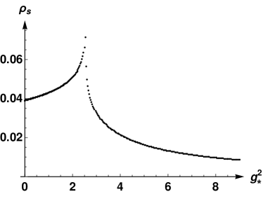
Figure 1: Shooting from the origin. Field coordinate $\rho_{s}$ of the singularity in $\zeta(\rho)$ closest to the origin as a function of $g^{2}$. Here $a=$1.7$$; the position of the spike provides $g_{m}^{2}(a=$1.7$)=$2.53$$.

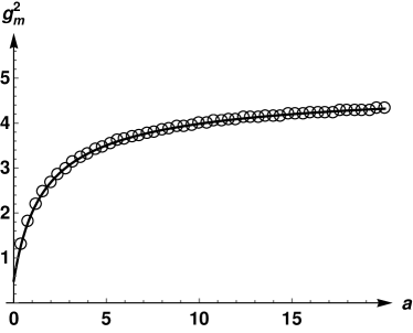
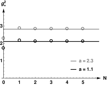
Figure 2: Left panel: Fixed point values $g_{m}^{2}$ as provided by shooting from the origin for different $a$. The solid line is a fit; for the interpolating function see Eq. (61). Right panel: Comparison of shooting from the origin and polynomial truncation. The solid line is located at $g_{m}^{2}(a)$ as obtained from the interpolating function. The $g_{*}^{2}(a,N)$ due to polynomial truncation of order $N$ converge to $g_{m}^{2}(a)$.

To go beyond polynomial truncations we first employ numerical integration by shooting from the origin. For each $g^{2}$ and $a$, the fixed-point equation (59) is a second-order nonlinear ordinary differential equation for $\zeta(\rho)$; hence we need to provide two initial conditions. Since we look for a solution that is smooth at the origin, the product $\rho\,\zeta^{\prime\prime}$ must vanish at $\rho=0$, which gives a closed relation between $g$ and $\zeta^{\prime}(0)$. Therefore, while one condition is determined by $\zeta(0)=1$, the second one, say $\zeta^{\prime}(0)$, can be parametrized by $g^{2}$. Yet, the normal form of Eq. (59) presents a $1/\rho\,$-pole at the origin, which we avoid by imposing our regular initial conditions at $\rho=\varepsilon\ll 1$.

Integrating Eq. (59) from $\rho=\varepsilon$ outwards, we constantly hit a movable singularity. As illustrated by Fig. 1, the position $\rho_{s}(g^{2})$ of this singularity exhibits a sharp maximum. Its location $g_{m}^{2}(a)$ is expected to correspond to the regular and polynomially bounded solution of the truncated fixed-point equation Hasenfratz and Hasenfratz (1986); Morris (1994b); Hellwig et al. (2015). The left panel of Fig. 2 shows the dependence of $g_{m}^{2}$ on $a$. We interpolate it using the fit

$$g_{m}^{2}(a)=\frac{$4.7951$a^{2}+$31.796$a-$5.2531$}{a^{2}+$9.0848$a-$10.624$}\,.$$ (61)

The right panel of Fig. 2 illustrates how the fixed-point values $g_{*}^{2}(a,N)$ obtained from the polynomial truncation (60) converge to $g_{m}^{2}(a)$.

Although shooting from the origin successfully predicts the unique critical $g_{*}^{2}$, it fails in producing a fixed-point Kähler metric which is globally defined in field space. The same applies to the polynomial truncation of Eq. (60), since it likewise represents an expansion about the origin. To obtain the global critical Kähler metric we employ pseudo-spectral methods, which are based on the expansion of $\zeta(\rho)$ in a basis of Chebyshev polynomials (see Refs. Borchardt and Knorr (2015, 2016) for applications to FRG equations). Though this is again a polynomial expansion, we derive the system of corresponding fixed-point equations not by a projection on the basis functions, but rather through a collocation method. To this end, it is convenient to map the $\rho$-domain into the compact interval $[0,1]$. Using a Gauss-grid in this interval, it is then possible to adopt a numerical relaxation method, such as for instance Newton-Raphson, to deduce the coefficients of $\zeta_{*}$ in the Chebyshev basis. Relaxation needs an initial seed, which is based on the information obtained with the polynomial and shooting methods.

The result of this analysis is presented in Fig. 3. It provides a smooth and featureless interpolation between the small-$\rho$ regime, which is satisfactorily described by the polynomial truncations and the shooting from the origin, and the large-$\rho$ region, where the Kähler metric is asymptotic to $\rho^{-\eta_{*}/(2\Delta_{*})}=\rho^{-1/4}$.

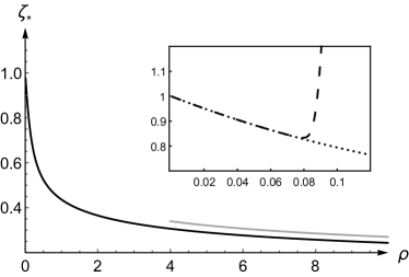
Figure 3: The critical Kähler metric for $a=$1.75$$. The solid black line is produced by pseudo-spectral methods, while the solid gray line shows a $\rho^{-1/4}$ decay. Inset: The pseudo-spectral solution (dotted line) is compared to the one obtained by shooting from the origin (dashed line) with $g_{*}^{2}=$2.576$$ corresponding to a maximum of $\rho_{s}$ as in Fig. 1.

VI.2 Critical exponent $\omega$

By tracking the RG flow of the Kähler metric, that is of infinitely many couplings which we expect to be irrelevant at the $\mathfrak{n}=3$ fixed point, we can extract estimates of many more universal quantities, i. e. eigenvalues of the linearized RG equations, which are related to correction-to-scaling exponents. As a case-study, we focus on $\omega$ to test the quality of different approximations.

We again start with a polynomial truncation. For generic perturbations of the fixed-point superpotential, which result in a $w_{*}+\delta w$ that is no longer a simple monomial, the Kähler metric is no longer a function of the single invariant $\rho$. Thus, in the polynomial truncation we refrain from combining $\chi$ and $\chi^{\dagger}$ into $\rho$:

$$\zeta(\chi,\chi^{\dagger})= \;1+\sum\limits_{n=1}^{N}\zeta_{n}(\chi\chi^{\dagger})^{n}$$ (62)

$$+\sum\limits_{n=0}^{N}\sum\limits_{m=1+n}^{2N-n}(\zeta_{nm}\chi^{n}\chi^{\dagger m}+\zeta_{mn}\chi^{m}\chi^{\dagger n})$$

with $\zeta_{n}^{\dagger}=\zeta_{n}$ and $\zeta_{mn}^{\dagger}=\zeta_{nm}$. The corresponding stability matrix conveys the linearized flow equations of both the superpotential and the Kähler metric. Hence it accounts for the couplings $c_{n}$, appearing in the superpotential, as well as $\zeta_{n}$ and $\zeta_{nm}$. For $r_{1}=0$, the stability matrix becomes block diagonal such that $g$ is coupled solely to $\{\zeta_{n}\}$. Restricting ourselves to this submatrix we can resort to the simplified flow equation (56) for $\zeta(\rho)$, still for $\eta=0$ on its right-hand side and the Litim-type regulator I from Eq. (58).

$N$	$a=$1.1$$	$a=$1.3$$	$a=$1.5$$	$a=$1.7$$	$a=$1.9$$	$a=$2.1$$	$a=$2.3$$
0	$1.0000$	$1.0000$	$1.0000$	$1.0000$	$1.0000$	$1.0000$	$1.0000$
1	$0.8270$	$0.8370$	$0.8422$	$0.8446$	$0.8454$	$0.8452$	$0.8444$
2	$0.8292$	$0.8310$	$0.8317$	$0.8317$	$0.8309$	$0.8298$	$0.8284$
3	$0.8258$	$0.8307$	$0.8330$	$0.8338$	$0.8338$	$0.8331$	$0.8321$
4	$0.8279$	$0.8319$	$0.8338$	$0.8345$	$0.8343$	$0.8336$	$0.8326$

Table 1: Critical exponent $\omega$ due to polynomial truncation of $\zeta(\rho)$ to order $N$.

Identifying the smallest positive eigenvalue of the stability submatrix with $\omega$ we obtain the results presented in Tab. 1. We have verified that all corresponding eigendirections indeed provide a non-vanishing $\delta g$. The computation of $\omega$ has turned out to be very memory-consuming. This has limited us in both the achievable truncation order $N$ and the step size of $a$. Yet we observe that, for all $N$, $\omega(a)$ exhibits a stationary point, whose position $a_{s}$ depends on $N$. At forth order the best approximation we have obtained is $\omega=$0.8345$$ at $a_{s}=$1.7$$. Convergence is achieved only for the first two significant figures.

Since polynomial truncations are computationally demanding, also for the determination of $\omega$ we again make use of shooting from the origin. Just as we linearized the flow equation of the superpotential in the fluctuations $\delta w=w-w_{*}$ and $\delta\eta=\eta-\eta_{*}$, obtaining Eq. (33), we can also linearize the flow of the Kähler metric with respect to $\delta w$, $\delta\eta$ and $\delta\zeta(\rho)=\zeta(\rho)-\zeta_{*}(\rho)$ to obtain a second-order linear partial differential equation. The eigendirections with $\delta w_{\lambda}\neq 0$, $\delta\zeta_{\lambda}=0$ are the ones already described in Eq. (35), for which no knowledge of $\delta\eta$ is required. The remaining perturbations with $\delta\zeta_{\lambda}\neq 0$ instead depend on $\delta\eta$, and according to our definitions must have $\delta\zeta(0)=0$. To extract $\omega$ we look for eigensolutions with $\lambda=\omega$ and

$$\delta w_{\omega}(\chi)=\frac{\delta g}{3}\,\chi^{3}.$$ (63)

Thus Eq. (33) and Eq. (34) can be analytically solved for $\delta g$ as a function of two unknowns: $\omega$ and $\delta\eta$. Then, the eigenvalue problem reduces to the solution of the single second-order ordinary differential equation for $\delta\zeta_{\omega}$, involving the two free parameters $\omega$ and $\delta\eta$. In addition, two initial conditions have to be supplied to specify a unique solution. We choose to provide them at the origin. As in the fixed point case, requiring the solution to be smooth at $\rho=0$ together with consistency between the initial conditions and the differential equation itself determines one of these conditions, say $\delta\zeta_{\omega}^{\prime}(0)$. Since the other one is provided by $\delta\zeta_{\omega}(0)=0$, the space of eigenfunctions is completely spanned by $\omega$ and $\delta\eta$.

While the former becomes quantized, by a mechanism that will be explained in the following, the latter remains a free parameter, as in the first order of the $\epsilon$ expansion, see Sec. V. Indeed, the considered differential equation is linear, such that the overall normalization of $\delta\zeta_{\omega}$ is arbitrary, and does not play a role in the determination of $\omega$. So, if the choice of $\delta\eta$ affects only the overall normalization of $\delta\zeta_{\omega}$, different values of $\omega$ correspond to genuinely different solutions. In particular, by inspecting the behavior of such solutions, one finds that they rapidly grow, with a rate that appears to be exponential. Indeed, these exponential parts are almost invariably present in solutions of linearized FRG equations. It is the additional requirement that the eigenfunctions $\delta\zeta_{\lambda}$ have to follow a power law for large $\rho$ that quantizes the set of possible eigenvalues. This requirement in turn is related to self-similarity Morris (1998) and to the existence of a well-defined norm in theory space Hamzaan Bridle and Morris (2016); O’Dwyer and Osborn (2008).

Thus, we expect a unique value of $\omega$ corresponding to a $\delta\zeta_{\omega}$ which is asymptotic to some power of $\rho$ for large $\rho$. In practice, a simple way to determine such a value consists in plotting $\delta\zeta_{\omega}(\rho_{L})$ as a function of $\omega$ for large enough $\rho_{L}$. Then, the solution with power-law asymptotic behavior should correspond to a special $\omega$ such that $\delta\zeta_{\omega}(\rho_{L})$ is exponentially smaller than for all other values outside a small neighborhood of it. We apply this criterion to the solutions constructed by shooting from the origin. In this case, each fixed-point solution extends over a finite range $[0,\rho_{s}]$. Therefore we parametrize $\rho_{L}=(1-\delta)\rho_{s}$, and scan over $\delta\ll 1$. We observe that $\delta\zeta_{\omega}(\rho_{L})$ as a function of $\omega$ shows only one zero, where it changes sign. This change of sign can be made arbitrarily quick by choosing smaller and smaller values of $\delta$. Its location converges to an unambiguous value in the limit $\delta\to 0$. This zero can be identified with the physical value of $\omega$. In the interval $a\in[$1.6$,$1.9$]$ we find $\omega=$0.834$$, with variations only in the fourth decimal place, showing a maximum at approximately $a=$1.8$$, where $\omega=$0.8344$$.

VII Momentum-dependent Kähler potential

Another branch of possible truncations is offered by the generalized Kähler potential with minimal field content:

$$\begin{split}\Gamma_{k}=&-\frac{Z_{0}}{4}\int\!\operatorname{d}^{d}\!x\operatorname{d}^{2}\!\theta\operatorname{d}^{2}\!\bar{\theta}\;\Phi^{\dagger}z(D,\bar{D})\Phi\\ &-\left\{\frac{1}{2i}\int\!\operatorname{d}^{d}\!x\operatorname{d}^{2}\!\theta\;W(\Phi)+\operatorname{h.\!c.}\right\}\end{split}$$ (64)

with analytic and Hermitian $z(D,\bar{D})$ fulfilling $z(0,0)=1$. Just as for the regulator functions $\rho_{2}$ and $r_{2}$ in (17) and (18), $z$ can be replaced by an analytic Hermitian generalized Kähler metric $\zeta(-\partial_{x}^{2})$ with $\zeta(0)=1$.

The flow of $\zeta$ can be obtained from the functional $\phi\,$- and $\phi^{\dagger}$- derivative of the FRG equation (14) at vanishing fields. $\Gamma_{k}^{(2)}(p,q)$ at constant $f$ and zero $\psi$, $\bar{\psi}$ is provided in App. D. Since it is no longer proportional to $\delta(p-q)$, $(\Gamma_{k}^{(2)}+R_{k})^{-1}$ cannot be computed just by matrix inversion. Hence, to evaluate the projection we proceed as described for instance in Ref. Gies and Wetterich (2002): We rewrite the flow equation (14) as

$$\partial_{t}\Gamma_{k}=\frac{1}{2}\operatorname{STr}\left(\tilde{\partial}_{t}\ln(\Gamma_{k}^{(2)}+R_{k})\right),$$ (65)

where $\tilde{\partial}_{t}$ is assumed to act on $R_{k}$ only, and expand the logarithm about the field independent part $\Gamma_{0}\propto\delta(p-q)$ of $\Gamma_{k}^{(2)}+R_{k}=:\Gamma_{0}+\Delta\Gamma$,

$$\begin{split}&\ln(\Gamma_{k}^{(2)}+R_{k})=\ln(\Gamma_{0})+\Gamma_{0}^{-1}\Delta\Gamma-\frac{1}{2}(\Gamma_{0}^{-1}\Delta\Gamma)^{2}+\ldots\,.\end{split}$$ (66)

Because every non-vanishing entry in $\Delta\Gamma$ is at least linear in $\phi$ or $\phi^{\dagger}$, we have to consider only addends containing $\Delta\Gamma$ once or twice.

The dimensionless, renormalized flow equation for $\zeta$ amounts to

$$(\partial_{t}-p\partial_{p}-\eta)\zeta(p^{2})=-\int\!\!\frac{\operatorname{d}^{d}\!q}{(2\pi)^{d}}\;\frac{4g^{2}h(q-p)}{v^{2}(q)v(q-p)}\times$$ (67)

$$\times\left[2hM(\partial_{t}-q\partial_{q}-\eta+1)r_{1}-u(\partial_{t}-q\partial_{q}-\eta)r_{2}\right](q)\,,$$

where all functions in the second line are evaluated at $q$. $M$, $u$ and $v$ are defined in Eq. (40) and $h=\zeta+r_{2}$. Discarding the momentum dependence of $\zeta$ in Eq. (67) restores the LPA^′ result of Eq. (39). At $d=2$ we recover the flow equation for the two-dimensional $\mathcal{N}=(2,2)$ WZ model derived in Ref. Synatschke-Czerwonka et al. (2010). The apparent discrepancy by a factor of two originates from a difference in the definitions of coupling constants and regulator functions. The flow equation (67) implies $\eta\propto g^{2}$, as becomes obvious when setting $p=0$. Hence, just as the LPA^′ truncation, it accounts only for the Gaussian and $\mathfrak{n}=3$ fixed points.

In the present paper we confine ourselves to the first-order polynomial truncation of the Kähler metric,

$$\zeta(p^{2})=1+p^{2}\zeta_{1}.$$ (68)

Thus, we have to consider the projections of Eq. (67) onto its zeroth and first orders in $p^{2}$. We report on the results obtained for the three-dimensional $\mathfrak{n}=3$ fixed point by adopting three different regulators. All arising integrals have been solved analytically. A further exploration of the ansatz in Eq. (64) is yet to be addressed.

We start with the Callan-Symanzik regulator defined in Eq. (45). Examining the vicinity of $\zeta_{1}=0$ at $\eta_{*}=1/3$ we numerically find the fixed point solution

$$(\zeta_{1*},\,g_{*}^{2})=($-0.0816$,\,$2.9425$).$$ (69)

The corresponding stability matrix couples $g$ to $c_{2}$ and $\zeta_{1}$. Its spectrum consists of Eq. (35) supplemented by the two eigenvalues

$$\omega=$0.6687$,\;\;\lambda_{\zeta}=$-75.75$.$$ (70)

We expect the additional relevant exponent $\lambda_{\zeta}$ to be an error induced by the combined effect of truncation and regularization scheme. This is supported by the results obtained with the other two regulators.

Despite its discontinuity in momentum space, the Litim-type regulator I, see Eq. (49), provides a finite flow of $\zeta_{1}$. The arising integrals converge for $\zeta_{1}>-1$. Note, however, that applying step-like regulators to higher orders of a $p^{2}$ expansion is problematic Bonanno et al. (1999); Canet et al. (2003b). Setting $\eta_{*}=1/3$ we numerically obtain the fixed point values

$$(\zeta_{1*},\,g_{*}^{2})=($-0.0138$,\,$1.9509$).$$ (71)

The stability matrix couples $g$ to $\zeta_{1}$. The corresponding eigenvalues evaluate to

$$\omega=$0.8317$,\;\;\lambda_{\zeta}=$2.530$.$$ (72)

To further simplify the flow equation we turn to another step-wise regulator, which we call the Litim-type regulator II. We set

$$r_{1}=0,\;\;r_{2}=\zeta(q^{2})\left(\frac{1}{q}\frac{\zeta(1)}{\zeta(q^{2})}-1\right)\Theta(1-q^{2}).$$ (73)

For $\zeta=1$ this coincides with our definition of Litim-type regulator I. With Eq. (73) again only low-energy modes, $q<1$, contribute to the flow, going along with $h(q)=\zeta(1)/q$ such that $u$ and $v$ become momentum-independent. Let us stress that, contrary to the other regulators adopted in this work, for the present choice the $\partial_{t}$-derivative on the right-hand side of Eq. (67) gives a non-vanishing contribution. The fixed point equation becomes

$$\begin{split}&35\zeta_{1*}(2+3\zeta_{1*})(1+\zeta_{1*})+(1+3\zeta_{1*})^{2}=0\,,\\ &g_{*}^{2}=\frac{2\pi^{2}}{5}\frac{(1+\zeta_{1*})^{3}}{2+3\zeta_{1*}}\,\end{split}$$ (74)

yielding three solutions. It is a common feature of polynomial truncations to suggest spurious fixed points. A comparison with our previous findings allows to identify the physical result as

$$\begin{split}g_{*}^{2}&=$1.9339$\,,\quad\quad\zeta_{1*}=$-0.0136$\,,\\ \omega&=$0.8443$\,,\quad\quad\,\,\lambda_{\zeta}=$2.411$\,.\end{split}$$ (75)

The good agreement between Eq. (72) and Eq. (75) suggests that we could qualitatively trust also the estimate of $\lambda_{\zeta}$. Finally, let us remark that the negative sign of $\zeta_{1*}$ does not necessarily signal the presence of negative norm states. In fact, within a polynomial truncation of $\zeta(p^{2})$ couplings with alternating signs are allowed and might be needed for convergence of the power series.

VIII Multicritical models

The critical models with $\mathfrak{n}>2$ can be constructed by using perturbation theory in vicinity of the upper critical dimensions $d_{\mathfrak{n}}$ defined in Eq. (32), where they are weakly coupled. In fact, if $d=d_{\mathfrak{n}}-\epsilon$ the constraint from Eq. (31) entails

$$\eta_{*}=\epsilon\frac{\mathfrak{n}-2}{\mathfrak{n}}\,.$$ (76)

This allows for a standard $\epsilon$ expansion in the spirit of Ref. Wilson and Kogut (1974). This approach has already been applied to non-supersymmetric multicritical models in fractional dimensions Itzykson and Drouffe (1989). Some of these studies have been performed directly in a FRG setup Nicoll et al. (1974); O’Dwyer and Osborn (2008); Codello et al. (2017).

For infinitesimal $\epsilon$ the deviations of the fixed-point values $w_{*}$ and $\zeta_{*}$ from the Gaussian ones $w_{*}=0$ and $\zeta_{*}=1$, as well as those of the eigenperturbations $\delta w$ and $\delta\zeta$ from the corresponding Gaussian eigenperturbations, behave as positive powers of $\epsilon$. Since the term $\eta\zeta$ on the left-hand side of Eq. (54) is of order $\epsilon$, we assume that the same holds for the right-hand side of this equation, i. e. we do not consider possible solutions with $(\zeta-1)$ of order $\epsilon^{P}$ with $P<1$. Instead, we assume that the power-counting in $\epsilon$ which we discussed for the $\mathfrak{n}=3$ model in Sec. V applies to any value of $\mathfrak{n}$.

In this case, the lowest order in Eq. (54) is of order $\epsilon$. This requires that $|c_{\mathfrak{n}*}|^{2}\propto\epsilon$ and, for $\mathfrak{n}>3$, also $\zeta^{\prime}\propto\epsilon$. It follows that at leading order the flow equation (54) becomes

$$\Big{(}\partial_{t}-\Delta_{\mathfrak{n}}\left(\chi\partial_{\chi}+\chi^{\dagger}\partial_{\chi^{\dagger}}\right)+l_{0\mathfrak{n}}\partial_{\chi}\partial_{\chi^{\dagger}}\Big{)}\zeta=\eta-l_{1\mathfrak{n}}|w^{\prime\prime\prime}|^{2}\,,$$ (77)

where $\Delta_{\mathfrak{n}}=(d_{\mathfrak{n}}-2)/2=1/(\mathfrak{n}-2)$ and we have defined the positive integrals

$$\begin{split}l_{0d}=\int_{q}\!\frac{(\partial_{t}-q\partial_{q})r_{2}}{(1+r_{2})^{2}q^{2}}\,,\\ l_{1d}=\int_{q}\!\frac{(\partial_{t}-q\partial_{q})r_{2}}{(1+r_{2})^{3}q^{4}}\,,\end{split}$$ (78)

which are denoted as $l_{0\mathfrak{n}}$ and $l_{1\mathfrak{n}}$ when evaluated at $d=d_{\mathfrak{n}}$. Let us stress that these numbers are, in general, regulator dependent. Only $l_{1\mathfrak{n}=3}$ is universal, since it corresponds to the one-loop anomalous dimension of the $\mathfrak{n}=3$ model. For $\mathfrak{n}>3$ the leading order of the $\epsilon$ expansion accounts for multi-loop diagrams. The ansatz of Eq. (53) is one-loop exact but it fails in reproducing all perturbative contributions beyond one loop. Thus, the $\epsilon$ expansion of Eq. (54) does not include all the contributions to leading order in $\epsilon$, which explains the appearance of nonuniversal coefficents. One can nevertheless extract approximate results from truncated and perturbatively expanded FRG equations, as is shown in Refs. Nicoll et al. (1974); O’Dwyer and Osborn (2008).

At the fixed point $|w_{*}^{\prime\prime\prime}|^{2}$ on the right-hand side of Eq. (77) depends on $\rho$ only, such that  Eq. (77) allows for radial solutions $\zeta_{*}(\rho)$. These are defined by a linear first-order ordinary differential equation for $\zeta_{*}^{\prime}(\rho)$. The physical solutions read

$$\zeta_{*}^{\prime}(\rho)=\epsilon\frac{\mathfrak{n}-2}{\mathfrak{n}\,l_{0\mathfrak{n}}}\sum_{i=0}^{\mathfrak{n}-4}\frac{1}{(i+1)!}\left(\frac{2\rho}{(\mathfrak{n}-2)l_{0\mathfrak{n}}}\right)^{i}\,.$$ (79)

The condition that $\zeta_{*}^{\prime}(0)$ be finite requires the cancellation of $1/\rho$ poles and fixes the coupling $c_{\mathfrak{n}}$ to the value

$$c_{\mathfrak{n}*}^{2}=\frac{\epsilon\ \left(l_{0\mathfrak{n}}/2\right)^{3-\mathfrak{n}}}{\mathfrak{n}(\mathfrak{n}-1)^{2}(\mathfrak{n}-2)^{\mathfrak{n}-2}(\mathfrak{n}-3)!\ l_{1\mathfrak{n}}}\,.$$ (80)

This is universal only for $\mathfrak{n}=3$. Since the radial fixed-point equation is a first-order ordinary differential equation, its space of solutions is parametrized by one integration constant, which we did not discuss so far. Indeed one could add to Eq. (79) a term of the form

$$\frac{K}{\rho}e^{\frac{2\rho}{(\mathfrak{n}-2)l_{0\mathfrak{n}}}}\,.$$ (81)

The constant $K$ has to be set to zero, to ensure that the space of perturbations of the fixed point possesses a well-defined norm, a countable basis and a discrete spectrum O’Dwyer and Osborn (2008); Hamzaan Bridle and Morris (2016).

Once the particular solution in Eq. (79) is known, it is possible to construct the general fixed-point solution through addition of the solutions of the homogeneous part of Eq. (77). The latter can be constructed by factoring the radial and the angular dependence, as will be detailed for the linear eigenperturbations in the following. The angular solutions are simple periodic functions $e^{i\mathfrak{m}\vartheta}$ labeled by the integer $\mathfrak{m}$. For any non-vanishing $\mathfrak{m}$, the radial component of the homogeneous solutions contains either a singularity at the origin or an exponentially growing part. We discard such solutions and set $\mathfrak{m}=0$.

Since at the upper critical dimension the fixed points are Gaussian, the eigenvalue problem for the linearized flow in the $\epsilon$ expansion can be interpreted as a perturbation of the Gaussian case. Therefore we first address the latter.

VIII.1 Linearized flow at the Gaussian fixed point

For the free theory, with $w_{*}=0$, $\eta_{*}=0$, and $\zeta_{*}=1$, the linearized flows of $\delta w$ and $\delta\zeta$ are decoupled, since Eq. (33) becomes independent of $\delta\eta$, while for the Kähler metric one finds

$$\partial_{t}\delta\zeta=\delta\eta+\left(\frac{d-2}{2}\left(\chi\partial_{\chi}+\chi^{\dagger}\partial_{\chi^{\dagger}}\right)-l_{0d}\partial_{\chi}\partial_{\chi^{\dagger}}\right)\delta\zeta\,.$$ (82)

Thus, there are separate families of eigendirections. Members of the first family have a perturbed superpotential only:

$$\begin{split}\delta w_{n}&=(\delta c_{n}\chi^{n})/n\,,\\ \lambda_{n}&=1-d+n\,\frac{d-2}{2}\,,\end{split}$$ (83)

and $\delta\zeta_{n}=\delta\eta_{n}=0$. Members of the second family have only a perturbed Kähler metric, which is conveniently expressed in spherical coordinates

$$\text{\calligra\Large r}=\sqrt{\frac{\rho}{l_{0}}}\,,\quad\vartheta=\arctan\left(i\,\frac{\chi^{\dagger}-\chi}{\chi^{\dagger}+\chi}\right)\,.$$ (84)

The eigenvalue problem in these coordinates reads

$$\left[\lambda-\frac{d-2}{2}\text{\calligra\Large r}\,\partial_{\!\text{\calligra\large r}}+\frac{1}{4}\left(\partial_{\!\text{\calligra\large r}}^{2}+\frac{1}{\!\text{\calligra\Large r}}\partial_{\!\text{\calligra\large r}}\right)+\frac{1}{4\text{\calligra\Large r}^{\,2}}\partial_{\vartheta}^{2}\right]\!\delta\zeta=\delta\eta\,.$$ (85)

Separable solutions can be obtained from the ansatz

$$\delta\zeta=\frac{\delta\eta}{\lambda}+e^{im\vartheta}\,Q(\kern-0.9pt\text{\calligra\Large r}\,)$$ (86)

giving rise to the following radial eigenvalue equation:

$$\left[\lambda-\frac{m^{2}}{4\text{\calligra\Large r}^{\,2}}-\frac{d-2}{2}\text{\calligra\Large r}\,\partial_{\!\text{\calligra\large r}}+\frac{1}{4}\left(\partial_{\!\text{\calligra\large r}}^{2}+\frac{1}{\!\text{\calligra\Large r}}\partial_{\!\text{\calligra\large r}}\right)\right]\!Q=0\,$$ (87)

Again, we constrain the space of solutions by prohibiting singularities at the origin and exponential growth for large radii. This eliminates half of the solutions and quantizes $\lambda$ to the following discrete spectrum:

$$\begin{split}\lambda_{km}&=(d-2)\left(k+\frac{|m|}{2}\right)\,,\quad k\in\mathbb{N}_{0}\,,\;\;m\in\mathbb{Z}\,\text{ even}\\ Q_{km}&=b_{km}\binom{k+|m|}{k}^{-1}\!\!\left((d-2)\text{\calligra\Large r}^{\,2}\right)^{\frac{|m|}{2}}\mathrm{L}_{k}^{|m|}\!\left((d-2)\text{\calligra\Large r}^{\,2}\right),\end{split}$$ (88)

where $\mathrm{L}$ denotes the generalized Laguerre polynomials and $b_{km}$ is an arbitrary normalization factor. The condition $\delta\zeta(0)=0$ determines $\delta\eta$:

$$\delta\zeta(0)=\frac{\delta\eta}{\lambda_{km}}+b_{km}\delta_{m0}=0,$$ (89)

such that the perturbations with $m=0$ can have a non-vanishing $\delta\eta$, which then scales with $b_{km}$. For all other eigendirections with $m\neq 0$ we have $\delta\eta=0$.

For special values of $d$, which are precisely of the form of $d_{\mathfrak{n}}$ in Eq. (32), provided

$$n=\mathfrak{n}+2k+|m|\,,$$ (90)

the two distinct subspaces of eigensolutions contain degenerate solutions going along with the same eigenvalue.

VIII.2 Critical exponent $\omega$ for general $\mathfrak{n}$

Let us now turn to the problem of determining the critical exponents of the multicritical models away from their upper critical dimensions. As the analysis in Sec. IV shows, the nonrenormalization of the superpotential imposes quantization rules for the critical $\eta$ and for the part of the spectrum described by Eq. (35). These can be straightforwardly rewritten using $d=d_{\mathfrak{n}}-\epsilon$ and provide eigenvalues that are linear in $\epsilon$, since $\Delta_{*}=\Delta_{\mathfrak{n}}-\epsilon/\mathfrak{n}$. In particular, they support the expectation that the number of physically relevant directions at the $\mathfrak{n}$-th fixed point be equal to $\mathfrak{n}-2$, though they do not describe the classically marginal case $n=\mathfrak{n}$. The latter has been already observed to become irrelevant for $\mathfrak{n}=3$ in the past sections. We now adopt the $\epsilon$ expansion to address this computation for generic $\mathfrak{n}$.

Integration of Eq. (33) for generic $\mathfrak{n}$ leads to

$$\delta w\!\left(\chi\right)=\frac{c_{\mathfrak{n}*}\delta\eta}{2\lambda}\chi^{\mathfrak{n}}+\delta c_{\lambda}\chi^{\mathfrak{n}+\frac{\mathfrak{n}\lambda}{d-1}}\,.$$ (91)

We focus on perturbations with $\delta c_{\lambda}=0$, which correspond to $\lambda=\omega$. As for the case $\mathfrak{n}=3$ discussed in Sec. V, to determine $\lambda$ additional knowledge from the running of $\zeta$ is needed. Before moving to the latter, let us stress that Eq. (35) and Eq. (91) can also be obtained by the $\epsilon$ expansion of the eigenvalue problem with the ansatz

$$\begin{split}\lambda&=\epsilon\,\lambda^{(1)}\,,\\ \delta\eta&=\sqrt{\epsilon}\,\delta\eta^{(1)}\,,\\ \delta w&=\delta w^{(0)}+\epsilon\,\delta w^{(1)}\,.\end{split}$$ (92)

At zeroth order in $\epsilon$ the Gaussian solution goes along with the eigenvalue $\lambda^{(0)}=0$, such that Eq. (91) relates the zeroth-order superpotential to the first-order eigenvalue by

$$\frac{\delta w_{\mathfrak{n}}^{(0)}}{\chi^{\mathfrak{n}}}=\frac{\delta c_{\mathfrak{n}}^{(0)}}{\mathfrak{n}}=\frac{c_{\mathfrak{n}*}\delta\eta}{2\lambda}\,.$$ (93)

where the right-hand side has to be expanded at lowest order in $\epsilon$.

Let us then turn to the perturbation of the Kähler metric. We complement Eq. (92) with

$$\delta\zeta=\sqrt{\epsilon}\,\delta\zeta^{(1)}\,.$$ (94)

Thus the leading non-trivial contribution in the $\epsilon$ expansion of the eigenvalue equation for $\delta\zeta$ is of order $\sqrt{\epsilon}$ and reads

$$\begin{split}\delta\eta\,+&\left(\Delta_{\mathfrak{n}}\left(\chi\partial_{\chi}+\chi^{\dagger}\partial_{\chi^{\dagger}}\right)-l_{0\mathfrak{n}}\partial_{\chi}\partial_{\chi^{\dagger}}\right)\delta\zeta=\\ &-2c_{\mathfrak{n}*}(\mathfrak{n}-1)^{2}(\mathfrak{n}-1)^{2}l_{1\mathfrak{n}}\delta c_{\mathfrak{n}}^{(0)}\rho^{\mathfrak{n}-3}\,.\end{split}$$ (95)

We first look for a special solution of this linear inhomogeneous partial differential equation, which in the spherical coordinates (84) is $\vartheta$-independent. The radial ansatz leads to a first order ordinary differential equation for $\delta\zeta^{\prime}(\kern-0.9pt\text{\calligra\Large r}\,)$. It possesses a one-parameter family of solutions, spanned by the same additive term of Eq. (81). As for the fixed point solution, we set this term to zero. This leads to the following radial solution

$$\delta\zeta^{\prime}(\kern-0.9pt\text{\calligra\Large r}\,)=2\delta\eta\,\sum_{i=1}^{\mathfrak{n}-3}\frac{\kern-0.9pt\text{\calligra\Large r}}{i!}\left(\frac{2\text{\calligra\Large r}^{\,2}}{\mathfrak{n}-2}\right)^{i-1}\,.$$ (96)

Here we have already imposed that $\delta\zeta^{\prime}(\kern-0.9pt\text{\calligra\Large r}\,)$ be smooth at the origin, which puts a constraint on $\delta\eta$, namely

$$\delta\eta=c_{\mathfrak{n}*}l_{1\mathfrak{n}}l_{0\mathfrak{n}}^{\mathfrak{n}-3}\frac{(\mathfrak{n}-1)^{2}(\mathfrak{n}-2)^{\mathfrak{n}-2}(\mathfrak{n}-2)!}{2^{\mathfrak{n}-4}}\delta c_{\mathfrak{n}}^{(0)}\,.$$ (97)

Compatibility between this relation and Eq. (93) determines $\lambda=\omega$ to be

$$\omega=(\mathfrak{n}-2)\epsilon,$$ (98)

where we have used Eq. (80). The fact that this result turns out to be universal suggests that it might agree with full perturbative computations.

Let us stress that the eigensolution (96) is a polynomial in r, while it shows a branch cut at the origin if expressed in terms of $\rho$. Since Eq. (96) represents a particular solution, one can construct the general eigensolution by adding the general solution of the associated homogeneous equation. The latter has, after separation of variables, the same form as Eq. (87), but with $\lambda=0$ and $d=d_{\mathfrak{n}}$. Since the only polynomial solutions are the ones in Eq. (88), for which $\lambda_{km}>0$, we conclude that Eq. (96) describes the only acceptable eigenperturbation corresponding to the eigenvalue of Eq. (98).

One might be tempted to compare the plain extrapolation of Eq. (98) at $\epsilon=d_{\mathfrak{n}}-2=2/(\mathfrak{n}-2)$ to the exact results known in two dimensions, in the hope of good agreement for large $\mathfrak{n}$. The agreement is not good at all, since we obtain $\omega=2$, while for the minimal models in two dimensions

$$\omega=\Delta_{\Phi\Phi^{\dagger}}+2-d=\frac{4}{\mathfrak{n}}\,$$ (99)

under the assumption that the lowest irrelevant scalar operator is related to $\Phi\Phi^{\dagger}$ by the action of the four supercharges Bobev et al. (2015b). This is because a resummation of the $\epsilon$ expansion is needed regardless of the numerical value of $\epsilon$ used in the plain extrapolation. Indeed such a disagreement had already been observed for the purely scalar models Itzykson and Drouffe (1989), and can be heuristically understood by considering that the actual expansion parameter is the classical dimension of the coupling $c_{\mathfrak{n}}$, i.e $(\mathfrak{n}-2)\epsilon/2$. The latter should be equal to one in two dimensions, and thus not small.

IX Conclusions

Three dimensional scale-invariant QFTs play a fundamental role as cornerstones in advancing and testing our understanding of strongly interacting QFTs. For instance, the Ising and the Gross-Neveu universality classes have been extensively analyzed for decades. Instead, comparatively few studies have addressed the WZ model with four supercharges, which in three dimensions defines what is sometimes called the supersymmetric Ising universality class. As an example, while the $\epsilon$ expansion about four dimensions has been computed up to six loops for the Ising case Schnetz (2016); Kompaniets and Panzer (2017), it has only recently been pushed up to three loops Zerf et al. (2016) and then four loops Zerf et al. (2017) for the nonsupersymmetric generalization of the present model. Other perturbative approaches have been adopted in the supersymmetric case. For instance, the four-dimensional WZ model has been studied up to four loops Avdeev et al. (1982), and the three-dimensional case up to two loops with the background field method Buchbinder et al. (2012). However, we do not know of any application of these computations to critical models.

As in the Ising phase transition, also in the supersymmetric case the two most interesting universal quantities are the critical exponents $\nu$ and $\eta$. The latter is exactly determined by supersymmetry Aharony et al. (1997), see Eq. (31). The former is defined in terms of the non-trivial supersymmetry-breaking relevant perturbation, roughly a change in the scalar mass at constant fermion bilinear. While supersymmetry cannot determine $\nu$, it provides an exact superscaling relation linking it to the first correction-to-scaling exponent on the supersymmetric hypersurface Thomas (2005), which we call $\omega$, namely

$$\omega=2-\frac{1}{\nu}\,.$$ (100)

The computation of this observable by means of the FRG has been the case study on which we have focused this exploratory work.

	O($\epsilon^{2}$)	O($\epsilon^{3}$)	O($\epsilon^{4}$)	Bootstrap	This Work
$\omega$	$0.667$	$0.909$	$0.871(1)$	$0.9098(20)$	$0.8344$

Table 2: The supersymmetric correction-to-scaling exponent at the $\mathcal{N}=2$ critical WZ model in three dimensions. See Sec. IX for explanations.

Before summarizing our results, let us first review what is known from the literature. The supersymmetric critical exponent $\omega$ has been computed at three loops in the $\epsilon$ expansion in Ref. Zerf et al. (2016), and at four loops in Ref. Zerf et al. (2017) which gives the result of Eq. (42). The numerical values that can be extracted from this expansion at different levels of approximation are presented in the first three columns of Tab. 2. For the two-loops approximation we give the plain extrapolation at $\epsilon=1$. For the three-loops computation we report the Padé $[1,2]$ or $[2,1]$ resummation of Ref. Fei et al. (2016). Finally the four-loops result has been used with the Padé approximants $[2,2]$ or $[3,1]$ in Ref. Zerf et al. (2017), obtaining $0.872$ or $0.870$ respectively, which we summarize as in the third column of Tab. 2. The fourth column shows the prediction of the conformal bootstrap Bobev et al. (2015a). The last entry presents our best estimate, obtained in Sec. VI.2. We are not able to estimate the systematic errors related to the truncation of the theory space, since we have not collected enough data on it. Yet we can select this result as the most accurate because it comes from the less restrictive truncation, accounting for a generic field-dependent Kähler metric. Furthermore, we have performed a minimal-sensitivity analysis of the regulator dependence, observing that its minimization is in fact a maximization of $\omega$. In Sec. VII we have also explored the alternative direction of including the momentum dependence of the generalized Kähler metric. Though in this case we were able to consider only two couplings, by changing the regulator we have obtained a maximal value $\omega=0.8317$, which further supports the result in Tab. 2.

In deriving these results, we have reproduced the known nonrenormalization of the superpotential. We have also compared our approximations to the perturbative $\epsilon$ expansion, finding that our flow equations not only exactly capture the one-loop contribution, but appear to perform better than the two-loops computation already in the simple approximation of a constant wave function renormalization, see Sec. V. This nicely illustrates how the FRG includes resummations of subsets of higher order diagrams. Yet, the truncations we have adopted appear to be still too poor to compete with three loops or the conformal bootstrap, since we are about 8$\%$ away from the results obtained by these methods. Higher orders of the derivative expansion might fill this gap. A proper numerical fixed-point analysis of the flow of Eq. (67) for the two-point function, i. e. the first order of a vertex expansion, might also yield better results.

The present FRG analysis of the critical three-dimensional WZ model thus leaves room for improvement in the determination of $\omega$, and furthermore does not address the computation of other properties of this scale-invariant model that can be found in the literature, e. g. the central charge or the sphere free energy Bobev et al. (2015b); Fei et al. (2016). Some of these can certainly be extracted with the RG method. It is furthermore possible to compute data on the operator product expansion, both within Sonoda (1993); Codello et al. (2017) or beyond perturbation theory Sonoda (1991); Pagani (2016); Pagani and Sonoda (2017). We leave such endeavors for future studies. Still, this work provides constructive evidence in favor of the existence of scale-invariant WZ models with four supercharges, in the form of explicit Landau-Ginzburg descriptions that go beyond the exact constraints imposed by the nonrenormalization of the superpotential. In fact, we have provided an approximation of the critical Kähler metric for an infinite tower of such models in continuous dimensions, as well as results showing that the scaling properties of these fixed points are genuinely non-Gaussian. This has been done in greater detail in Sec. VI.1 for the three-dimensional $\mathcal{N}=2$ case, where we have determined the critical Kähler metric by means of local and global numerical methods.

In Sec. VIII we have also presented a partial perturbative analysis of multicritical models between two and three dimensions, with superpotential $W\propto\Phi^{\mathfrak{n}}$, employing an $\epsilon$ expansion of truncated FRG equations around the corresponding upper critical dimensions. Apart from constructing fixed-point solutions, we have computed the exponent $\omega$ at first order in $\epsilon$, see Eq. (98). Collecting information supporting the existence of such non-Gaussian fixed points in continuous dimensions could seem a purely academic exercise. Yet, there might be hope to experimentally test such phenomena through intriguing relations between short range statistical models in fractional dimensions and long range ones in integer dimensions Defenu et al. (2015). For the multicritical models, the present study does not address many interesting aspects. In particular, we are not aware of a full $\epsilon$ expansion, and nonperturbative FRG analyses in two or continuous dimensions are missing.

Of course, the RG equations we have computed can be employed to study off-critical features of these models, such as supersymmetry breaking, or the finite temperature and density phase diagram. Also, they can be used to search for unknown critical models that are not revealed by a simple analysis of the superpotential, such as for instance theories with shift symmetry or with a quadratic superpotential (e. g. the $\mathfrak{n}=1$ and $\mathfrak{n}=2$ cases in Eq. (31)). It would also be interesting to perform an FRG analysis of models with several superfields. Finally, similar FRG studies might shed some light on the nature of the putative minimal four-dimensional $\mathcal{N}=1$ superconformal theory observed in conformal-bootstrap studies, see Refs. Poland et al. (2012); Bobev et al. (2015b); Poland and Stergiou (2015); Xie and Yonekura (2016); Li et al. (2017).

Appendix A Dirac Conventions

In four-dimensional flat spacetime we adopt the signature $(1,-1,-1,-1)$ such that $\Gamma^{0}$ is Hermitian and $\Gamma^{i}$ is anti-Hermitian. As usual, $\bar{\psi}$ denotes the Dirac conjugate $\bar{\psi}=\psi^{\dagger}\Gamma^{0}$. We set

$$\Gamma_{5}:=-i\Gamma_{0}\Gamma_{1}\Gamma_{2}\Gamma_{3}.$$ (101)

After dimensional reduction to the three-dimensional Euclidean space the metric has signature $(1,1,1)$, and the Dirac conjugate becomes

$$\bar{\psi}\equiv\psi^{\dagger}.$$ (102)

The integrals over anticommuting variables, occurring in the superfield formulations of Lagrangian densities, see e. g. Eq. (10), denote a Berezin integration with

$$\operatorname{d}^{2}\!\theta\equiv\operatorname{d}\!\theta_{1}\operatorname{d}\!\theta_{2},\;\operatorname{d}^{2}\!\bar{\theta}\equiv\operatorname{d}\!\bar{\theta}_{2}\operatorname{d}\!\bar{\theta}_{1}.$$ (103)

Note that each $\operatorname{d}\!\theta_{i}$, $\operatorname{d}\!\bar{\theta}_{i}$ has mass dimension $1/2$.

For Dirac spinors and their conjugates we use the same Fourier transform conventions as for bosons:

$$f(q)=\frac{1}{\sqrt{2\pi}^{d}}\int\!\operatorname{d}^{d}\!x\;f(x)\operatorname{e}^{iqx}\,.$$ (104)

More details on conventions and computations can be found in Ref. Feldmann (2016).

Appendix B LPA^′

Within the ansatz of Eq. (37) the bosonic block of $\Gamma_{k}^{(2)}$ at constant bosonic fields and vanishing fermionic field is sufficient to obtain $\partial_{t}Z_{0}$ and $\partial_{t}W$. It reads

$$\Gamma_{B}^{(2)}=\begin{pmatrix}q^{2}Z_{0}&-{W^{\dagger}}^{\prime\prime\prime}f^{\dagger}&0&-{W^{\dagger}}^{\prime\prime}\\ -W^{\prime\prime\prime}f&q^{2}Z_{0}&-W^{\prime\prime}&0\\ 0&-{W^{\dagger}}^{\prime\prime}&-Z_{0}&0\\ -W^{\prime\prime}&0&0&-Z_{0}\end{pmatrix}\delta(p-q).$$ (105)

The computation of $\partial_{t}Z_{0}$ proceeds by projecting Eq. (14) onto zero fields $\phi,\psi$ and auxiliary fields $f(x)=f\delta(x)$ and subsequently evaluating $(\partial_{f^{\dagger}}\partial_{f})$ at $f=0$. The off-diagonal blocks of $\Gamma_{k}^{(2)}$ which mix bosons and fermions vanish at $\psi=0$, while the fermionic block is not needed since it carries no dependence on $f$ or $f^{\dagger}$.

Appendix C Kähler Potential

To extract the flow of the Kähler metric from Eq. (14) within the ansatz of Eq. (53) we, once more, start out from constant fields and vanishing $\psi$. Denoted in component fields, Eq. (53) reads

$$\begin{split}\Gamma_{k}=&\int\!\operatorname{d}^{d}\!x\left\{Z_{0}\left[\zeta\,\Big{(}|\nabla\phi|^{2}+\frac{i}{2}\bar{\psi}\not{\sigma}\psi-\frac{i}{2}(\partial_{j}\bar{\psi})\sigma^{j}\psi-ff^{\dagger}\Big{)}\right.\right.\\ &\qquad\left.\left.+\frac{1}{2}\Big{(}\partial_{\phi}\zeta\left(\psi^{T}\sigma^{2}\psi f^{\dagger}+i\bar{\psi}\sigma^{j}\psi\partial_{j}\phi\right)+\operatorname{h.\!c.}\Big{)}\right.\right.\\ &\qquad\left.\left.-\frac{1}{2}\partial_{\phi}\partial_{\phi^{\dagger}}\zeta\psi^{T}\sigma^{2}\psi\bar{\psi}\sigma^{2}\psi^{*}\right]\right.\\ &\left.-\left(W^{\prime}(\phi)f-\frac{1}{2}W^{\prime\prime}(\phi)\psi^{T}\sigma^{2}\psi+\operatorname{h.\!c.}\right)\right\}.\end{split}$$ (106)

Its second variation at constant bosonic fields and $\psi=0$ consists of two diagonal blocks,

$$\begin{split}\Gamma_{B}^{(2)}&=\delta(p-q)F_{B}(Z_{0},q^{2},\zeta,f,f^{\dagger})\,,\\ \Gamma_{F}^{(2)}&=\delta(p-q)F_{f}(Z_{0},q_{j},\zeta,f,f^{\dagger})\,,\end{split}$$ (107)

with field-dependent $\zeta$. For more details on these matrices see Ref. Feldmann (2016). The flow of the Kähler metric is obtained from $(\partial_{f^{\dagger}}\partial_{f})$ at $f=0$ and reads

$$\begin{split}&\left(\partial_{t}+\frac{\Delta}{2}\big{(}\chi^{\dagger}\partial_{\chi^{\dagger}}-\chi\partial_{\chi}\big{)}+\eta\right)\zeta(\chi,\chi^{\dagger})=-\int_{q}\frac{1}{v^{3}}\\ &\left\{\vphantom{\frac{i}{2}}(\partial_{t}-q\partial_{q}-\eta+1)r_{1}\right.\\ &\left.\Big{[}h^{2}(M+M^{\dagger})|w^{\prime\prime\prime}|^{2}-h\Big{(}(2M^{\dagger 2}+u)w^{\prime\prime\prime}\partial_{\chi^{\dagger}}\zeta+\operatorname{h.c.}\Big{)}\right.\\ &\left.+(M+M^{\dagger})\Big{(}(u-2q^{2}h^{2})|\partial_{\chi}\zeta|^{2}+hv\partial_{\chi}\partial_{\chi^{\dagger}}\zeta\Big{)}\Big{]}\right.\\ &\left.+(\partial_{t}-q\partial_{q}-\eta)r_{2}\right.\\ &\left.\Big{[}-hu|w^{\prime\prime\prime}|^{2}+(u-2q^{2}h^{2})\left(M^{\dagger}w^{\prime\prime\prime}\partial_{\chi^{\dagger}}\zeta+\operatorname{h.c.}\right)\right.\\ &\left.+2q^{2}h(2|M|^{2}+u)|\partial_{\chi}\zeta|^{2}-uv\partial_{\chi}\partial_{\chi^{\dagger}}\zeta\,\Big{]}\vphantom{\frac{i}{2}}\right\}\end{split}$$ (108)

with the abbreviations

$$\begin{split}h&=\zeta+r_{2},\;\;\quad\quad\quad\;\;\;M=w^{\prime\prime}+r_{1}\,,\\ u&=|M|^{2}-q^{2}h^{2},\;\;\quad\;\,\,\,v=|M|^{2}+q^{2}h^{2}\,,\end{split}$$ (109)

and the notation of Eq. (38). Setting $\zeta(\phi,\phi^{\dagger})=1$ recovers the LPA^′ result. We have confirmed the flow of the Kähler metric by deriving it also from the projection onto the fermionic kinetic term.

C.1 Fixed Point Couplings

The three Tables 3, 4, and 5 contain, for an exemplary set of values of the prefactor $a$ in the regulator (58), the fixed point results obtained by polynomially truncating $\zeta(\rho)$ up to order $N$, as in Eq. (60).

$N$	$g_{*}^{2}$	$\zeta_{1*}$	$\zeta_{2*}$	$\zeta_{3*}$	$\zeta_{4*}$	$\zeta_{5*}$
0	$1.7233$	0	0	0	0	0
1	$2.1749$	$-3.3423$	0	0	0	0
2	$2.1308$	$-3.0161$	$8.2007$	0	0	0
3	$2.1334$	$-3.0357$	$7.7102$	$-14.842$	0	0
4	$2.1325$	$-3.0290$	$7.8779$	$-9.7650$	$132.56$	0
5	$2.1328$	$-3.0313$	$7.8194$	$-11.537$	$86.305$	$-1121.5$

Table 3: Fixed point couplings due to polynomial truncation of $\zeta_{*}(\rho)$ to order $N$; $a=$1.1$$.

$N$	$g_{*}^{2}$	$\zeta_{1*}$	$\zeta_{2*}$	$\zeta_{3*}$	$\zeta_{4*}$	$\zeta_{5*}$
0	$2.0714$	0	0	0	0	0
1	$2.5856$	$-2.7795$	0	0	0	0
2	$2.5501$	$-2.5877$	$4.5557$	0	0	0
3	$2.5479$	$-2.5756$	$4.8418$	$7.6240$	0	0
4	$2.5482$	$-2.5773$	$4.8009$	$6.5346$	$-25.835$	0
5	$2.5483$	$-2.5777$	$4.7908$	$6.2655$	$-32.219$	$-139.07$

Table 4: Fixed point couplings due to polynomial truncation of $\zeta_{*}(\rho)$ to order $N$; $a=$1.7$$.

$N$	$g_{*}^{2}$	$\zeta_{1*}$	$\zeta_{2*}$	$\zeta_{3*}$	$\zeta_{4*}$	$\zeta_{5*}$
0	$2.2929$	0	0	0	0	0
1	$2.8865$	$-2.6793$	0	0	0	0
2	$2.8413$	$-2.4752$	$4.5749$	0	0	0
3	$2.8384$	$-2.4624$	$4.8619$	$7.1570$	0	0
4	$2.8391$	$-2.4656$	$4.7905$	$5.3765$	$-39.590$	0
5	$2.8392$	$-2.4658$	$4.7847$	$5.2318$	$-42.807$	$-65.562$

Table 5: Fixed point couplings due to polynomial truncation of $\zeta_{*}(\rho)$ to order $N$; $a=$2.3$$.

Appendix D Momentum Dependence

The second variation $\Gamma_{k}^{(2)}(p,q)$ of ansatz (64) at constant $f$ and vanishing Fermi-field is block-diagonal with

$$\Gamma_{B}^{(2)}=\left(\begin{array}[]{cc}q^{2}Z_{0}\zeta\delta(p-q)&-\kappa W^{\prime\prime\prime\dagger}(p-q)f^{\dagger}\\ -\kappa W^{\prime\prime\prime}(p-q)f&q^{2}Z_{0}\zeta\delta(p-q)\\ 0&-\kappa W^{\prime\prime\dagger}(p-q)\\ -\kappa W^{\prime\prime}(p-q)&0\end{array}\right.\\ \cdots\left.\begin{array}[]{cc}0&-\kappa W^{\prime\prime\dagger}(p-q)\\ -\kappa W^{\prime\prime}(p-q)&0\\ -Z_{0}\zeta\delta(p-q)&0\\ 0&-Z_{0}\zeta\delta(p-q)\end{array}\right)$$ (110)

and

$$\Gamma_{F}^{(2)}=\begin{pmatrix}Z_{0}\zeta\sigma^{j}q_{j}\delta(p-q)&\kappa W^{\prime\prime\dagger}(p-q)\sigma^{2}\\ \kappa W^{\prime\prime}(p-q)\sigma^{2}&Z_{0}\zeta\sigma^{jT}q_{j}\delta(p-q)\end{pmatrix},$$ (111)

where $\kappa=(2\pi)^{-3/2}$.

References

- Wess and Zumino (1974) J. Wess and B. Zumino, Phys. Lett. 49B, 52 (1974).
- Fateev and Zamolodchikov (1985) V. A. Fateev and A. B. Zamolodchikov, Sov. Phys. JETP 62, 215 (1985), [Zh. Eksp. Teor. Fiz.89,380(1985)].
- Di Vecchia et al. (1986) P. Di Vecchia, J. L. Petersen, M. Yu, and H. B. Zheng, Phys. Lett. B174, 280 (1986).
- Mussardo et al. (1989) G. Mussardo, G. Sotkov, and M. Stanishkov, Int. J. Mod. Phys. A4, 1135 (1989).
- Cecotti and Vafa (1993a) S. Cecotti and C. Vafa, Commun. Math. Phys. 157, 139 (1993a), arXiv:hep-th/9209085 [hep-th] .
- Cecotti and Vafa (1993b) S. Cecotti and C. Vafa, Commun. Math. Phys. 158, 569 (1993b), arXiv:hep-th/9211097 [hep-th] .
- Vafa and Warner (1989) C. Vafa and N. P. Warner, Phys. Lett. B218, 51 (1989).
- Bienkowska (1993) J. Bienkowska, Int. J. Mod. Phys. A8, 3945 (1993), arXiv:hep-th/9109003 [hep-th] .
- Iliopoulos and Zumino (1974) J. Iliopoulos and B. Zumino, Nucl. Phys. B76, 310 (1974).
- Grisaru et al. (1979) M. T. Grisaru, W. Siegel, and M. Rocek, Nucl. Phys. B159, 429 (1979).
- Seiberg (1993) N. Seiberg, Phys. Lett. B318, 469 (1993), arXiv:hep-ph/9309335 [hep-ph] .
- Flume and Kraus (2000) R. Flume and E. Kraus, Nucl. Phys. B569, 625 (2000), arXiv:hep-th/9907120 [hep-th] .
- Rosenstein et al. (1991) B. Rosenstein, B. Warr, and S. H. Park, Phys. Rept. 205, 59 (1991).
- Gracey (1993) J. A. Gracey, Phys. Lett. B308, 65 (1993), arXiv:hep-th/9305012 [hep-th] .
- Gracey (1994) J. A. Gracey, Phys. Rev. D50, 2840 (1994), [Erratum: Phys. Rev.D59,109904(1999)], arXiv:hep-th/9406162 [hep-th] .
- Kleinert and Babaev (1998) H. Kleinert and E. Babaev, Phys. Lett. B438, 311 (1998), arXiv:hep-th/9809112 [hep-th] .
- Karkkainen et al. (1994) L. Karkkainen, R. Lacaze, P. Lacock, and B. Petersson, Nucl. Phys. B415, 781 (1994), [Erratum: Nucl. Phys.B438,650(1995)], arXiv:hep-lat/9310020 [hep-lat] .
- Hands et al. (1993) S. Hands, A. Kocic, and J. B. Kogut, Annals Phys. 224, 29 (1993), arXiv:hep-lat/9208022 [hep-lat] .
- Hands et al. (1995) S. Hands, S. Kim, and J. B. Kogut, Nucl. Phys. B442, 364 (1995), arXiv:hep-lat/9501037 [hep-lat] .
- Barbour et al. (1999) I. Barbour, S. Hands, J. B. Kogut, M.-P. Lombardo, and S. Morrison, Nucl. Phys. B557, 327 (1999), arXiv:hep-lat/9902033 [hep-lat] .
- Hands et al. (2001) S. J. Hands, J. B. Kogut, and C. G. Strouthos, Phys. Lett. B515, 407 (2001), arXiv:hep-lat/0107004 [hep-lat] .
- Christofi and Strouthos (2007) S. Christofi and C. Strouthos, JHEP 05, 088 (2007), arXiv:hep-lat/0612031 [hep-lat] .
- Chandrasekharan and Li (2013) S. Chandrasekharan and A. Li, Phys. Rev. D88, 021701 (2013), arXiv:1304.7761 [hep-lat] .
- Hesselmann and Wessel (2016) S. Hesselmann and S. Wessel, Phys. Rev. B93, 155157 (2016), arXiv:1602.02096 [cond-mat.str-el] .
- Strassler (2003) M. J. Strassler, in Strings, Branes and Extra Dimensions: TASI 2001: Proceedings (2003) pp. 561–638, arXiv:hep-th/0309149 [hep-th] .
- Aharony et al. (1997) O. Aharony, A. Hanany, K. A. Intriligator, N. Seiberg, and M. J. Strassler, Nucl. Phys. B499, 67 (1997), arXiv:hep-th/9703110 [hep-th] .
- Thomas (2005) S. Thomas, “Emergent supersymmetry,” KITP talk (2005).
- Lee (2007) S.-S. Lee, Phys. Rev. B76, 075103 (2007), arXiv:cond-mat/0611658 [cond-mat] .
- Lee (2010) S.-S. Lee, in Proceedings, Theoretical Advanced Study Institute in Elementary Particle Physics (TASI 2010). String Theory and Its Applications: From meV to the Planck Scale: Boulder, Colorado, USA, June 1-25, 2010 (2010) pp. 667–706, arXiv:1009.5127 [hep-th] .
- Ponte and Lee (2014) P. Ponte and S.-S. Lee, New J. Phys. 16, 013044 (2014), arXiv:1206.2340 [cond-mat.str-el] .
- Grover et al. (2014) T. Grover, D. N. Sheng, and A. Vishwanath, Science 344, 280 (2014), arXiv:1301.7449 [cond-mat.str-el] .
- Sonoda (2011) H. Sonoda, Prog. Theor. Phys. 126, 57 (2011), arXiv:1102.3974 [hep-th] .
- Fei et al. (2016) L. Fei, S. Giombi, I. R. Klebanov, and G. Tarnopolsky, PTEP 2016, 12C105 (2016), arXiv:1607.05316 [hep-th] .
- Zerf et al. (2016) N. Zerf, C.-H. Lin, and J. Maciejko, Phys. Rev. B94, 205106 (2016), arXiv:1605.09423 [cond-mat.str-el] .
- Gies et al. (2017) H. Gies, T. Hellwig, A. Wipf, and O. Zanusso, (2017), arXiv:1705.08312 [hep-th] .
- Zhao and Liu (2017) P.-L. Zhao and G.-Z. Liu, (2017), arXiv:1706.02231 [cond-mat.str-el] .
- Bobev et al. (2015a) N. Bobev, S. El-Showk, D. Mazac, and M. F. Paulos, Phys. Rev. Lett. 115, 051601 (2015a), arXiv:1502.04124 [hep-th] .
- Bobev et al. (2015b) N. Bobev, S. El-Showk, D. Mazac, and M. F. Paulos, JHEP 08, 142 (2015b), arXiv:1503.02081 [hep-th] .
- Jafferis (2012) D. L. Jafferis, JHEP 05, 159 (2012), arXiv:1012.3210 [hep-th] .
- Imamura and Yokoyama (2012) Y. Imamura and D. Yokoyama, Phys. Rev. D85, 025015 (2012), arXiv:1109.4734 [hep-th] .
- Closset et al. (2013) C. Closset, T. T. Dumitrescu, G. Festuccia, and Z. Komargodski, JHEP 05, 017 (2013), arXiv:1212.3388 [hep-th] .
- Nishioka and Yonekura (2013) T. Nishioka and K. Yonekura, JHEP 05, 165 (2013), arXiv:1303.1522 [hep-th] .
- Wilson and Kogut (1974) K. G. Wilson and J. B. Kogut, Phys. Rept. 12, 75 (1974).
- Wegner and Houghton (1973) F. J. Wegner and A. Houghton, Phys. Rev. A8, 401 (1973).
- Berges et al. (2002) J. Berges, N. Tetradis, and C. Wetterich, Phys. Rept. 363, 223 (2002), arXiv:hep-ph/0005122 [hep-ph] .
- Kopietz et al. (2010) P. Kopietz, L. Bartosch, and F. Schütz, Lect. Notes Phys. 798, 1 (2010).
- Gies (2012) H. Gies, ECT* School on Renormalization Group and Effective Field Theory Approaches to Many-Body Systems Trento, Italy, February 27-March 10, 2006, Lect. Notes Phys. 852, 287 (2012), arXiv:hep-ph/0611146 [hep-ph] .
- Rosa et al. (2001) L. Rosa, P. Vitale, and C. Wetterich, Phys. Rev. Lett. 86, 958 (2001), arXiv:hep-th/0007093 [hep-th] .
- Hofling et al. (2002) F. Hofling, C. Nowak, and C. Wetterich, Phys. Rev. B66, 205111 (2002), arXiv:cond-mat/0203588 [cond-mat] .
- Strack et al. (2010) P. Strack, S. Takei, and W. Metzner, Phys. Rev. B81, 125103 (2010), arXiv:0905.3894 [cond-mat.str-el] .
- Gies et al. (2010) H. Gies, L. Janssen, S. Rechenberger, and M. M. Scherer, Phys. Rev. D81, 025009 (2010), arXiv:0910.0764 [hep-th] .
- Braun et al. (2011) J. Braun, H. Gies, and D. D. Scherer, Phys. Rev. D83, 085012 (2011), arXiv:1011.1456 [hep-th] .
- Scherer and Gies (2012) D. D. Scherer and H. Gies, Phys. Rev. B85, 195417 (2012), arXiv:1201.3746 [cond-mat.str-el] .
- Janssen and Gies (2012) L. Janssen and H. Gies, Phys. Rev. D86, 105007 (2012), arXiv:1208.3327 [hep-th] .
- Janssen and Herbut (2014) L. Janssen and I. F. Herbut, Phys. Rev. B89, 205403 (2014), arXiv:1402.6277 [cond-mat.str-el] .
- Gehring et al. (2015) F. Gehring, H. Gies, and L. Janssen, Phys. Rev. D92, 085046 (2015), arXiv:1506.07570 [hep-th] .
- Vacca and Zambelli (2015) G. P. Vacca and L. Zambelli, Phys. Rev. D91, 125003 (2015), arXiv:1503.09136 [hep-th] .
- Classen et al. (2016) L. Classen, I. F. Herbut, L. Janssen, and M. M. Scherer, Phys. Rev. B93, 125119 (2016), arXiv:1510.09003 [cond-mat.str-el] .
- Classen et al. (2017) L. Classen, I. F. Herbut, and M. M. Scherer, (2017), arXiv:1705.08973 [cond-mat.str-el] .
- Synatschke et al. (2010) F. Synatschke, J. Braun, and A. Wipf, Phys. Rev. D81, 125001 (2010), arXiv:1001.2399 [hep-th] .
- Heilmann et al. (2015) M. Heilmann, T. Hellwig, B. Knorr, M. Ansorg, and A. Wipf, JHEP 02, 109 (2015), arXiv:1409.5650 [hep-th] .
- Hellwig et al. (2015) T. Hellwig, A. Wipf, and O. Zanusso, Phys. Rev. D92, 085027 (2015), arXiv:1508.02547 [hep-th] .
- Heilmann et al. (2012) M. Heilmann, D. F. Litim, F. Synatschke-Czerwonka, and A. Wipf, Phys. Rev. D86, 105006 (2012), arXiv:1208.5389 [hep-th] .
- Rosten (2010) O. J. Rosten, JHEP 03, 004 (2010), arXiv:0808.2150 [hep-th] .
- Sonoda and Ulker (2010) H. Sonoda and K. Ulker, Prog. Theor. Phys. 123, 989 (2010), arXiv:0909.2976 [hep-th] .
- Osborn and Twigg (2012) H. Osborn and D. E. Twigg, Annals Phys. 327, 29 (2012), arXiv:1108.5340 [hep-th] .
- Synatschke-Czerwonka et al. (2010) F. Synatschke-Czerwonka, T. Fischbacher, and G. Bergner, Phys. Rev. D82, 085003 (2010), arXiv:1006.1823 [hep-th] .
- Wetterich (1993) C. Wetterich, Phys. Lett. B301, 90 (1993).
- Morris (1994a) T. R. Morris, Int. J. Mod. Phys. A9, 2411 (1994a), arXiv:hep-ph/9308265 [hep-ph] .
- Ellwanger (1994) U. Ellwanger, Proceedings, Workshop on Quantum field theoretical aspects of high energy physics: Bad Frankenhausen, Germany, September 20-24, 1993, Z. Phys. C62, 503 (1994), [,206(1993)], arXiv:hep-ph/9308260 [hep-ph] .
- Bonini et al. (1993) M. Bonini, M. D’Attanasio, and G. Marchesini, Nucl. Phys. B409, 441 (1993), arXiv:hep-th/9301114 [hep-th] .
- Bonini and Vian (1998) M. Bonini and F. Vian, Nucl. Phys. B532, 473 (1998), arXiv:hep-th/9802196 [hep-th] .
- Synatschke et al. (2009a) F. Synatschke, G. Bergner, H. Gies, and A. Wipf, JHEP 03, 028 (2009a), arXiv:0809.4396 [hep-th] .
- Feldmann (2016) P. Feldmann, Functional Renormalization Group Approach to the 3-Dimensional N = 2 Wess-Zumino Model, Master’s thesis, Jena U., TPI (2016).
- Synatschke et al. (2009b) F. Synatschke, H. Gies, and A. Wipf, Phys. Rev. D80, 085007 (2009b), arXiv:0907.4229 [hep-th] .
- Bardeen et al. (1985) W. A. Bardeen, K. Higashijima, and M. Moshe, Nucl. Phys. B250, 437 (1985).
- Litim et al. (2011) D. F. Litim, M. C. Mastaler, F. Synatschke-Czerwonka, and A. Wipf, Phys. Rev. D84, 125009 (2011), arXiv:1107.3011 [hep-th] .
- Bardeen et al. (1984) W. A. Bardeen, M. Moshe, and M. Bander, Phys. Rev. Lett. 52, 1188 (1984).
- Comellas and Travesset (1997) J. Comellas and A. Travesset, Nucl. Phys. B498, 539 (1997), arXiv:hep-th/9701028 [hep-th] .
- Marchais et al. (2017) E. Marchais, P. Mati, and D. F. Litim, Phys. Rev. D95, 125006 (2017), arXiv:1702.05749 [hep-th] .
- Gies and Zambelli (2015) H. Gies and L. Zambelli, Phys. Rev. D92, 025016 (2015), arXiv:1502.05907 [hep-ph] .
- Gies and Zambelli (2016) H. Gies and L. Zambelli, (2016), arXiv:1611.09147 [hep-ph] .
- Zerf et al. (2017) N. Zerf, L. N. Mihaila, P. Marquard, I. F. Herbut, and M. M. Scherer, Phys. Rev. D96, 096010 (2017), arXiv:1709.05057 [hep-th] .
- Liao et al. (2000) S.-B. Liao, J. Polonyi, and M. Strickland, Nucl. Phys. B567, 493 (2000), arXiv:hep-th/9905206 [hep-th] .
- Litim (2000) D. F. Litim, Phys. Lett. B486, 92 (2000), arXiv:hep-th/0005245 [hep-th] .
- Litim (2001a) D. F. Litim, The exact renormalization group. Proceedings, 2nd Conference, Rome, Italy, September 18-22, 2000, Int. J. Mod. Phys. A16, 2081 (2001a), arXiv:hep-th/0104221 [hep-th] .
- Litim (2001b) D. F. Litim, Phys. Rev. D64, 105007 (2001b), arXiv:hep-th/0103195 [hep-th] .
- Canet et al. (2003a) L. Canet, B. Delamotte, D. Mouhanna, and J. Vidal, Phys. Rev. D67, 065004 (2003a), arXiv:hep-th/0211055 [hep-th] .
- Synatschke et al. (2009c) F. Synatschke, G. Bergner, H. Gies, and A. Wipf, Journal of High Energy Physics 2009, 028 (2009c).
- Hasenfratz and Hasenfratz (1986) A. Hasenfratz and P. Hasenfratz, Nuclear Physics B 270, 687 (1986).
- Morris (1994b) T. R. Morris, Phys. Lett. B334, 355 (1994b), arXiv:hep-th/9405190 [hep-th] .
- Borchardt and Knorr (2015) J. Borchardt and B. Knorr, Phys. Rev. D91, 105011 (2015), [Erratum: Phys. Rev.D93,no.8,089904(2016)], arXiv:1502.07511 [hep-th] .
- Borchardt and Knorr (2016) J. Borchardt and B. Knorr, Phys. Rev. D94, 025027 (2016), arXiv:1603.06726 [hep-th] .
- Morris (1998) T. R. Morris, Nonperturbative QCD: Structure of the QCD vacuum: Proceedings, Yukawa International Seminar, YKIS’97, Kyoto, Japan, December 2-12, 1997, Prog. Theor. Phys. Suppl. 131, 395 (1998), arXiv:hep-th/9802039 [hep-th] .
- Hamzaan Bridle and Morris (2016) I. Hamzaan Bridle and T. R. Morris, Phys. Rev. D94, 065040 (2016), arXiv:1605.06075 [hep-th] .
- O’Dwyer and Osborn (2008) J. O’Dwyer and H. Osborn, Annals Phys. 323, 1859 (2008), arXiv:0708.2697 [hep-th] .
- Gies and Wetterich (2002) H. Gies and C. Wetterich, Phys. Rev. D 65, 065001 (2002).
- Bonanno et al. (1999) A. Bonanno, V. Branchina, H. Mohrbach, and D. Zappala, Phys. Rev. D60, 065009 (1999), arXiv:hep-th/9903173 [hep-th] .
- Canet et al. (2003b) L. Canet, B. Delamotte, D. Mouhanna, and J. Vidal, Phys. Rev. B68, 064421 (2003b), arXiv:hep-th/0302227 [hep-th] .
- Itzykson and Drouffe (1989) C. Itzykson and J. M. Drouffe, STATISTICAL FIELD THEORY. VOL. 1: FROM BROWNIAN MOTION TO RENORMALIZATION AND LATTICE GAUGE THEORY (1989).
- Nicoll et al. (1974) J. F. Nicoll, T. S. Chang, and H. E. Stanley, Phys. Rev. Lett. 33, 540 (1974).
- Codello et al. (2017) A. Codello, M. Safari, G. P. Vacca, and O. Zanusso, (2017), arXiv:1705.05558 [hep-th] .
- Schnetz (2016) O. Schnetz, (2016), arXiv:1606.08598 [hep-th] .
- Kompaniets and Panzer (2017) M. V. Kompaniets and E. Panzer, Phys. Rev. D96, 036016 (2017), arXiv:1705.06483 [hep-th] .
- Avdeev et al. (1982) L. V. Avdeev, S. G. Gorishnii, A. Yu. Kamenshchik, and S. A. Larin, Phys. Lett. 117B, 321 (1982).
- Buchbinder et al. (2012) I. L. Buchbinder, B. S. Merzlikin, and I. B. Samsonov, Nucl. Phys. B860, 87 (2012), arXiv:1201.5579 [hep-th] .
- Sonoda (1993) H. Sonoda, Nucl. Phys. B394, 302 (1993), arXiv:hep-th/9205084 [hep-th] .
- Sonoda (1991) H. Sonoda, Nucl. Phys. B352, 585 (1991).
- Pagani (2016) C. Pagani, Phys. Rev. D94, 045001 (2016), arXiv:1603.07250 [hep-th] .
- Pagani and Sonoda (2017) C. Pagani and H. Sonoda, (2017), arXiv:1707.09138 [hep-th] .
- Defenu et al. (2015) N. Defenu, A. Trombettoni, and A. Codello, Phys. Rev. E92, 052113 (2015), arXiv:1409.8322 [cond-mat.stat-mech] .
- Poland et al. (2012) D. Poland, D. Simmons-Duffin, and A. Vichi, JHEP 05, 110 (2012), arXiv:1109.5176 [hep-th] .
- Poland and Stergiou (2015) D. Poland and A. Stergiou, JHEP 12, 121 (2015), arXiv:1509.06368 [hep-th] .
- Xie and Yonekura (2016) D. Xie and K. Yonekura, Phys. Rev. Lett. 117, 011604 (2016), arXiv:1602.04817 [hep-th] .
- Li et al. (2017) D. Li, D. Meltzer, and A. Stergiou, JHEP 07, 029 (2017), arXiv:1702.00404 [hep-th] .