SNe 2013K and 2013am: observed and physical properties of two slow, normal Type IIP events

Abstract

We present one year of optical and near-infrared photometry and spectroscopy of the Type IIP SNe 2013K and 2013am. Both objects are affected by significant extinction, due to their location in dusty regions of their respective host galaxies, ESO 009-10 and NGC 3623 (M65). From the photospheric to nebular phases, these objects display spectra congruent with those of underluminous Type IIP SNe (i.e. the archetypal SNe 1997D or 2005cs), showing low photospheric velocities ($\sim 2\times 10^{3}$ km s^-1 at 50 d) together with features arising from Ba II which are particularly prominent in faint SNe IIP. The peak $V$-band magnitudes of SN 2013K ($-15.6$ mag) and SN 2013am ($-16.2$ mag) are fainter than standard-luminosity Type IIP SNe. The ejected Nickel masses are $0.012\pm 0.010$ and $0.015\pm 0.006$ M_⊙ for SN 2013K and SN 2013am, respectively. The physical properties of the progenitors at the time of explosion are derived through hydrodynamical modelling. Fitting the bolometric curves, the expansion velocity and the temperature evolution, we infer total ejected masses of 12 and 11.5 M_⊙, pre-SN radii of $\sim 460$ and $\sim 360$ R_⊙, and explosion energies of 0.34 foe and 0.40 foe for SN 2013K and SN 2013am. Late time spectra are used to estimate the progenitor masses from the strength of nebular emission lines, which turn out to be consistent with red supergiant progenitors of $\sim 15$ M_⊙. For both SNe, a low-energy explosion of a moderate-mass red supergiant star is therefore the favoured scenario.

1 Introduction

Type II plateau supernovae (SNe IIP) are thought to be the explosive end-stages of H-rich massive stars (above 8 M_⊙; see e.g. Woosley & Weaver 1986; Heger et al. 2003; Pumo et al. 2009). From an observational point of view, these SNe are characterised by the presence of broad hydrogen lines with P-Cygni profiles in their spectra, and a long-lasting ($\sim 100$ d) plateau in the light curve, while the hydrogen recombination wave propagates inside the SN ejecta. At the end of the plateau phase, there is a sudden drop of luminosity in the bolometric curve to meet the radioactive tail, which is characterised by a linear decline of 0.98 mag (100 d)^-1, and where the electromagnetic emission is powered by the decay of ⁵⁶Co to ⁵⁶Fe.

Numerical simulations of such photometric properties suggest that Type IIP SNe originate from red-supergiant stars (RSGs; see for example Grassberg, Imshennik, & Nadyozhin, 1971; Falk & Arnett, 1977; Woosley & Weaver, 1986; Heger et al., 2003; Utrobin, 2007; Pumo & Zampieri, 2011, 2013; Dessart et al., 2013, and references therein). This association has been confirmed by the detection of several RSGs as precursors of Type IIP SNe in pre-explosion images (e.g. Smartt 2009 for a review). However, some disagreement on progenitor masses remains, and there is a general trend for masses coming from hydrodynamical modelling to be higher than those determined from pre-SN imaging (see Utrobin & Chugai, 2008; Smartt et al., 2009b; Smartt, 2015b). Furthermore, it is not known how the observed diversity in both photometric and spectroscopic properties of SNe IIP depends on their progenitor properties (Hamuy, 2003; Dessart et al., 2013; Anderson et al., 2014; Faran et al., 2014; Sanders et al., 2015; Galbany et al., 2016; Valenti et al., 2016; Rubin et al., 2016; Gal-Yam, 2017). At early epochs, there is a wide range between standard-luminosity SNe IIP (characterised by an average peak magnitude of $M_{V}=-16.74$ mag with $\sigma=1.01$, see Anderson et al., 2014) and low-luminosity events, down to $\sim-15$ mag (Pastorello et al., 2004; Spiro et al., 2014). SN 1997D was the first underluminous SN IIP (Turatto et al. 1998, Benetti et al. 2001), followed by a growing number of similar events (Hamuy, 2003; Pastorello et al., 2004; Pastorello et al., 2009; Utrobin, 2007; Fraser et al., 2011; Van Dyk et al., 2012; Arcavi, Gal-Yam, & Sergeev, 2013; Spiro et al., 2014). In the “middle ground” only few intermediate-luminosity SNe have been studied (i.e. SN 2008in, SN 2009N, SN 2009js, SN 2009ib, SN 2010id, SN 2012A, see Roy et al., 2011; Takáts et al., 2014; Gandhi et al., 2013; Takáts et al., 2015; Gal-Yam et al., 2011; Tomasella et al., 2013, respectively).

Typically, these intermediate-luminosity SNe also show low expansion velocities that match those of the extremely faint SNe IIP, while their late time light curves indicate ⁵⁶Ni masses ranging between those of the Ni-poor underluminous objects (less than $10^{-2}$ M_⊙ of ⁵⁶Ni) and more canonical values ($0.06$ to $0.10$ M_⊙ of ⁵⁶Ni; cf. Müller et al. 2017, Anderson et al. 2014). Overall, the observational properties of intermediate SNe IIP suggest a continuous distribution of Type IIP properties. The cause of the observed spread of parameters among faint, intermediate and standard SNe IIP still remains unclear.

In this paper we present observational data and hydrodynamical modelling for a pair of intermediate-luminosity objects, SN 2013K and SN 2013am. These events first caught our interest due to their relatively low expansion velocities and intrinsic magnitudes. The earliest classification spectra of SN 2013K (Taddia et al., 2013) and SN 2013am (Benetti et al., 2013) were similar to the underluminous Type IIP SN 2005cs (Pastorello et al., 2006; Pastorello et al., 2009), showing ejecta velocities of about 6300 and 8500 km s^-1, respectively, from the H${\beta}$ absorption minima. For both SNe, we immediately started extensive campaigns of photometric and spectroscopic monitoring, lasting over one year. These campaigns were enabled by the Public ESO Survey of Transient Objects (PESSTO, Smartt et al. 2015) and the Asiago Classification Program (ACP, Tomasella et al., 2014), supported also by other facilities. Over the course of the photometric follow-up campaign, it became apparent that the luminosity and duration of the plateau-phase for SNe 2013K and 2013am are closers to those of the intermediate-luminosity Type IIP SNe, matching SN 2012A (Tomasella et al., 2013) rather than more extreme sub-luminous Type IIP SNe. We note that optical data for SN 2013am (complemented by public Swift $UV$ photometry) have been previously reported by Zhang et al. (2014).

Our motivation for a comparative study of the almost identical SNe 2013K and 2013am, is to expand the sample of well-studied intermediate-luminosity events in the literature, and with that to help understanding the physical causes behind the observed diversity in Type IIP SNe. To this end, we determine the physical parameters of the progenitors at the point of explosion through hydrodynamical modelling of the SN observables (i.e. bolometric light curve, evolution of line velocities and continuum temperature at the photosphere, see Pumo, Zampieri, & Turatto, 2010; Pumo & Zampieri, 2011; Pumo et al., 2017). Also, we use the observed nebular spectra, and in particular the luminosities of the forbidden lines of Oxygen and Calcium or Nickel and Iron, to constrain the main-sequence mass of the progenitors (Fransson & Chevalier, 1989; Maguire et al., 2012; Jerkstrand et al., 2012; Jerkstrand et al., 2015).

The paper is organised as follows: in Section 2 we report basic information on the detection of SN 2013K and SN 2013am. Optical, near-infrared (NIR), ultraviolet ($UV$) observations together with a description of the data reduction process are provided in Section 3. In Section 4, we present the optical and NIR photometric evolution of the two SNe, comparing their colour and bolometric light curves with those of other Type IIP SNe, deriving the ejected Nickel masses from the bolometric radioactive tail, and analysing the spectroscopic data from photospheric to nebular phases. Section 5 is devoted to hydrodynamical modelling. Finally, in Section 6 we discuss and summarise the main results of our study.

2 The two SNe and their host galaxies

In Table 1, we summarise the main observational data for SNe 2013K and 2013am and their host galaxies. The Tully-Fisher distance moduli reported in the Nasonova, de Freitas Pacheco, & Karachentsev (2011) catalogue of $32.66\pm 0.40$ mag for SN 2013K and $30.54\pm 0.40$ mag for SN 2013am (adopting $H_{0}$ = $73\pm 5$ km s^-1 Mpc^-1) are used throughout this paper. The foreground Galactic extinctions $A_{B}$ = 0.516 mag and $A_{B}$ = 0.090 mag adopted for SNe 2013K and 2013am, respectively, are from Schlafly & Finkbeiner (2011). For the estimation of the total extinction (Galactic plus host galaxy) see Section 4.2.

2.1 SN 2013K

The discovery of SN 2013K, close to the nucleus of the southern galaxy ESO 009-10 (Fig. 1), was reported by S. Parker (Backyard Observatory Supernova Search - BOSS) on 2013 Jan. 20.413 UT (UT will be used hereafter in the paper). The transient was classified by Taddia et al. (2013) on behalf of the PESSTO collaboration (see Smartt et al., 2015) as a Type II SN a few days past maximum light. The explosion epoch is not well defined, as the closest non-detection image was taken by S. Parker on 2012 Dec. 9.491 at a limiting magnitude 18. The template-matching approach applied to the early spectra, using the GELATO and SNID spectral classification tools (Harutyunyan et al., 2008; Blondin & Tonry, 2007), and the light-curve, allow to constrain the explosion epoch to be around 2013 Jan. 9, with a moderate uncertainty (MJD = $56302.5^{+5}_{-5}$). After the classification, we promptly triggered a PESSTO follow-up campaign on this target.

2.2 SN 2013am

SN 2013am was first detected by Nakano et al. (2013) in M65 (NGC 3623, see Fig. 2) on 2013 Mar. 21.638 UT. It was classified as a young SN II by Benetti et al. (2013) under the Asiago Classification Program (ACP, Tomasella et al., 2014). There was no evidence of the SN (down to an unfiltered magnitude $\sim$19) on frames taken by the Catalina Real-time Transient Survey (CRTS) on Mar. 20.198, indicating that the SN was caught very early. This stringent non-detection constrains the explosion time with a small uncertainty. In this paper, we adopt Mar. 21.0 (MJD = $56371.5^{+1.5}_{-1.0}$) as the explosion epoch. After the classification, we initiated a joint PESSTO and Asiago programme follow-up campaign on this target.

Table 1: Main data for SNe 2013am and 2013K, and the respective host galaxies, M 65 and ESO 009-10.

	SN 2013am	SN 2013K
Host galaxy	M 65	ESO 009-10
Galaxy type	SABa	SAbc
Heliocentric velocity (km s-1)	$807\,\pm\,3$	$2418\,\pm\,10$
Distance (Mpc)	12.8	34.0
Distance modulus (mag)	$30.54\,\pm\,0.40$	$32.66\,\pm\,0.40$
Galactic extinction $A_{B}$ (mag)	0.090	0.516
Total extinction $A_{B},A_{V},E(B-V)$ (mag)	$\approx$2.5, 2.0, $0.65\pm 0.10$	$\approx$1.0, 0.7, $0.25\pm 0.20$
SN Type	IIP	IIP
RA(J2000.0)	11h18m56.95s	17h39m31.54s
Dec(J2000.0)	+13∘03′49$\aas@@fstack{\prime\prime}$4	$-85^{\circ}$18′38$\aas@@fstack{\prime\prime}$1
Offset from nucleus	15$\aas@@fstack{\prime\prime}$E 102$\aas@@fstack{\prime\prime}$S	6$\aas@@fstack{\prime\prime}$E 1$\aas@@fstack{\prime\prime}$S
Date of discovery UT	2013 Mar. 21.64	2013 Jan. 20.41
Date of discovery (MJD)	56372.6	56312.4
Estimated date of explosion (MJD)	$56371.5^{+1.5}_{-1.0}$	$56302.0^{+5}_{-5}$
$m_{V}$ at maximum (mag)	$16.34\,\pm\,0.01$	$17.67\,\pm\,0.04$
$M_{V}$ at maximum (mag)	$-16.2\,\pm\,0.3$	$-15.6\,\pm\,0.2$
$L_{\rm bol}$ peak ($\times 10^{41}$ erg s-1)	15.0${}^{+2.2}_{-2.0}$	5.2${}^{+2.5}_{-1.6}$ (UV missing)

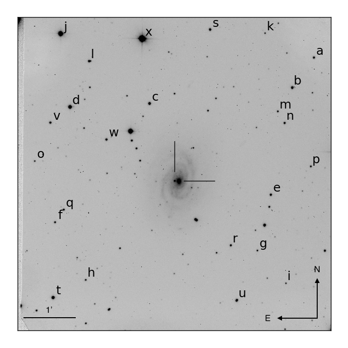
Figure 1: SN 2013K (located 6 arcsec East and 1 arcsec South of the center of ESO 009-10) and local sequence stars (CTIO SMARTS 1.3m Telescope, $R$-band image obtained on 2013 Feb. 12, with exposure time 150s).

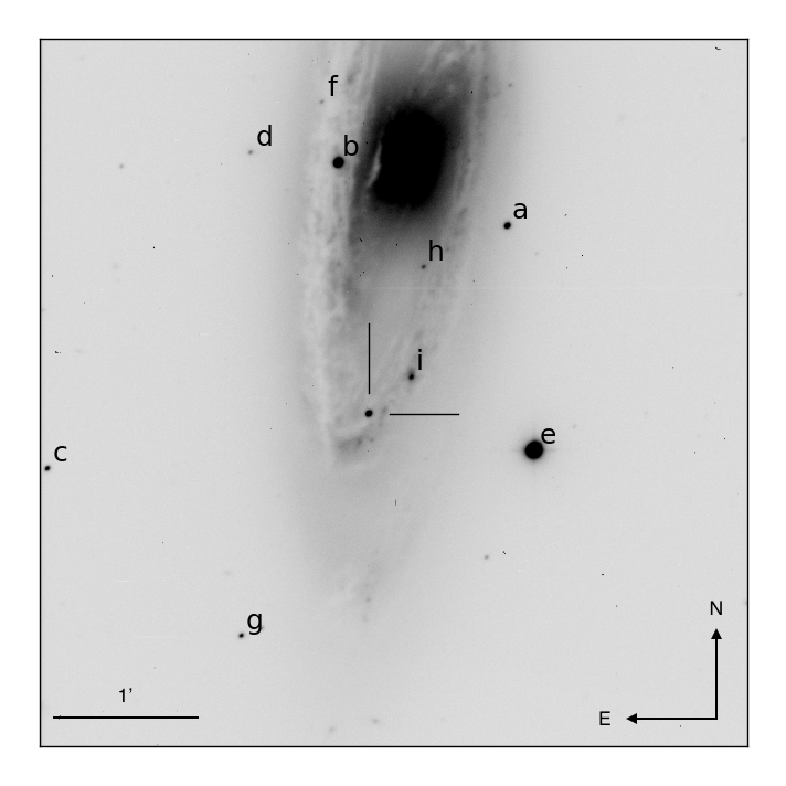
Figure 2: SN 2013am and local sequence stars (Liverpool Telescope, $g$-band image obtained on 2013 Mar. 30, with exposure time 180s).

3 Observations and data reduction

3.1 Photometry

Table 2: List of observing facilities employed for optical and infrared photometry.

Telescope	Instrument	Site	FoV	Scale
			[arcmin2]	[arcsec pix-1]
Optical facilities
Schmidt 67/92cm	SBIG	Asiago, Mount Ekar (Italy)	$57\times 38$	0.86
Copernico 1.82m	AFOSC	Asiago, Mount Ekar (Italy)	$8\times 8$	0.48
Prompt 41cm	PROMPT	CTIO Observatory (Chile)	$11\times 11$	0.59
SMARTS 1.3m	ANDICAM-CCD	CTIO Observatory (Chile)	$6\times 6$	0.37
LCO 1.0m	kb73, kb74	CTIO Observatory (Chile)	$16\times 16$	0.47
LCO 1.0m	kb77	McDonald Observatory, Texas (USA)	$16\times 16$	0.47
LCO FTS 2.0m	fs01	Siding Spring (Australia)	$10\times 10$	0.30
LCO FTN 2.0m	fs02	Haleakala, Hawai (USA)	$10\times 10$	0.30
Liverpool 2.0m LT	RATCam	Roque de los Muchachos, La Palma, Canary Islands (Spain)	$4.6\times 4.6$	0.135
Trappist 60cm	TRAPPISTCAM	ESO La Silla Observatory (Chile)	$27\times 27$	0.65
ESO NTT 3.6m	EFOSC2	ESO La Silla Observatory (Chile)	$4\times 4$	0.24
TNG 3.6m	LRS	Roque de los Muchachos, La Palma, Canary Islands (Spain)	$8\times 8$	0.25
Infrared facilities
REM 60cm	REMIR	ESO La Silla Observatory (Chile)	$10\times 10$	1.22
ESO NTT 3.6m	SOFI	ESO La Silla Observatory (Chile)	$5\times 5$	0.29
NOT 2.56m	NOTCam	Roque de los Muchachos, La Palma, Canary Islands (Spain)	$4\times 4$	0.234
SMARTS 1.3m	ANDICAM-IR	CTIO Observatory (Chile)	$2.4\times 2.4$	0.276

Optical and near infrared (NIR) photometric monitoring of SNe 2013am and 2013K was obtained using multiple observing facilities, summarised in Table 2. For SN 2013am, we collected data using Johnson-Cousins UBVRI, Sloan ugriz plus JHK filters. For SN 2013K mostly BVRI-band images were taken, with only three epochs in $U$ (obtained with NTT$+$EFOSC2; photometric standard fields were also observed during these nights), and four in gri bands. The latter, covering the critical phase from the end of the plateau to the beginning of the radioactive tail, were transformed to VRI (Vega) magnitudes using relations from Chonis & Gaskell (2008).

All frames were pre-processed using standard procedures in iraf for bias subtraction, flat fielding and astrometric calibration. For NIR, illumination correction and sky background subtraction were applied. For later epochs, multiple exposures obtained in the same night and with the same filter were combined to improve the signal-to-noise ratio. The photometric calibration of the two SNe was done relative to the sequences of stars in the field (Figs 1 and 2) and calibrated using observations either of Landolt (1992) or Sloan Digital Sky Survey (SDSS, Data Release 12, Alam et al. 2015) fields. The local sequences (see Table 3) were used to compute zero-points for non-photometric nights. In the NIR, stars from the 2MASS catalogue were used as photometric reference. The SN magnitudes have been measured via point-spread-function (PSF) fitting using a dedicated pipeline (snoopy package, Cappellaro 2014). snoopy is a collection of python scripts calling standard iraf tasks (through pyraf) and specific data analysis tools such as sextractor for source extraction and daophot for PSF fitting. The sky background at the SN location is first estimated with a low-order polynomial fit of the surrounding area. Then, the PSF model derived from isolated field stars is simultaneously fitted to the SN and any point source projected nearby (i.e. any star-like source within a radius of $\sim 5\times$FWHM from the SN). The fitted sources are removed from the original images, an improved estimate of the local background is derived and the PSF fitting procedure iterated. The residuals are visually inspected to validate the fit. Error estimates were derived through artificial star experiments. In this procedure, fake stars with magnitudes similar to the SN are placed in the fit residual image at a position close to, but not coincident with, the SN location. The simulated image is processed through the same PSF fitting procedure and the standard deviation of the recovered magnitudes of a number of artificial star experiments is taken as an estimate of the instrumental magnitude error. For a typical SN, this is mainly a measure of the uncertainty in the background fitting. The instrumental error is combined (in quadrature) with the PSF fit error, and the propagated errors from the photometric calibration chain.

Johnson-Bessell, Sloan optical magnitudes and NIR photometry of both SNe (and associated errors) are listed in Tables 4, 6, 7, 8, 9 and 10. Magnitudes are in the Vega system for the Johnson-Bessell filters, and in the AB system for the Sloan filters.

An alternative technique for transient photometry is template subtraction. However, this requires the use of exposures of the field obtained before the SN explosion or after the SN has faded below the detection threshold. The template images should be taken with the same filter, and with good signal to noise and seeing. In principle, they should be obtained with the same telescope and instrumental set-up, but in practice we are limited to what is actually available in the public archives. We retrieved pre-discovery SDSS ri-band exposures covering M65, the host of SN 2013am. The template (SDSS) images were geometrically registered to the same pixel grid as the SN ones, and the PSFs matched by means of a convolution kernel determined from reference sources in the field. Then, the template image was subtracted from the SN frame and the difference image was used to measure the transient magnitude. Comparing the PSF fitting vs. template subtraction, the measured values differ by less than 0.1 mag. We considered this to be a satisfactory agreement given the differences between the passband of template (Sloan ri) and SN images (Johnson-Bessell RI). We conclude that our PSF fitting magnitudes are properly corrected for background contamination at least in the case of SN 2013am.

The light curves of SN 2013am were complemented with $UV$-optical photometry (at eleven epochs, from phases $+2$ d to $+29$ d) obtained with the Ultra-Violet/Optical Telescope (UVOT; Roming et al., 2005) onboard the Swift spacecraft (Gehrels et al., 2004). The data were retrieved from the Swift Data Center and were re-calibrated in 2016 using version 2015.1 of Peter Brown’s photometry pipeline and version swift_Rel4.5(Bld34)_27Jul2015 of HEASOFT (Brown et al., 2014; Brown, Roming, & Milne, 2015). The reduction is based on the work of Brown et al. (2009), including subtraction of the host galaxy count rates and uses the revised $UV$ zero-points and time-dependent sensitivity from Breeveld et al. (2011). We note that the photometry of Zhang et al. (2014) for SN 2013am is systematically brighter in RI during the radioactive tail phase. The reason for this discrepancy is unclear, and we only include the photometry earlier than 109 d from Zhang et al. when computing the pseudo-bolometric light curve.

3.2 Spectroscopy

The journals of spectroscopic observations for SNe 2013K and 2013am, both optical and NIR, are reported in Tables 11 and 12 respectively.

Data reduction was performed using standard iraf tasks. First, images were bias and flat-field corrected. Then, the SN spectrum was extracted, subtracting the sky background along the slit direction. One-dimensional spectra were extracted weighting the signal by the variance based on the data values and a Poisson/CCD model using the gain and readout-noise parameters. The extracted spectra have been wavelength-calibrated using comparison lamp spectra and flux-calibrated using spectrophotometric standard stars observed, when possible, in the same night and with the same instrumental configuration as the SN. The flux calibration of all spectra was verified against photometric measures and, if necessary, corrected. The telluric absorptions were corrected using the spectra of both telluric and spectrophotometric standards.

All PESSTO spectra collected with the 3.6m New Technology Telescope (NTT+EFOSC2 or NTT+SOFI, cf. Tables 11 and 12) are available through the ESO Science Archive Facility. Full details of the formats of these spectra can be found on the PESSTO website and in Smartt et al. (2015). Some spectra were obtained under the ANU WiFeS SuperNovA Programme, which is an ongoing supernova spectroscopy campaign utilising the Wide Field Spectrograph on the Australian National University 2.3-m telescope. The first and primary data release of this programme (AWSNAP-DR1, see Childress et al., 2016) releases 357 spectra of 175 unique objects collected over 82 equivalent full nights of observing from 2012 Jul. to 2015 Aug. These spectra have been made publicly available via the Weizmann Interactive Supernova data REPository (WISeREP, Yaron & Gal-Yam 2012).

4 Data analysis

4.1 Light curves

The multicolour light curves of SN 2013K and SN 2013am are shown in Figs 3 and 4, respectively. The unfiltered discovery magnitudes are also included (Taddia et al., 2013; Nakano et al., 2013) and plotted as empty squares on the $R$-band light curves. For SN 2013am, a polynomial fit to the early light curves shows that the $B$- and $V$-band maxima are reached about 5 and 8 days after the explosion at $m_{B}=17.05\pm 0.03$ mag and $m_{V}=16.34\pm 0.01$ mag, respectively, in fair agreement with the estimate by Zhang et al. (2014). At subsequent epochs, we note a steep decline in the $B$ band ($\approx 3.76\pm 0.13$ mag (100 d)^-1) during the first 50 d of evolution, and a moderate decline in the $V$ band ($\approx 0.68\pm 0.05$ mag (100 d)^-1). The $R$ light curve shows a flat evolution during the first $\sim$ 85 d, with $m_{R}=15.72\pm 0.03$ mag, followed by the sharp luminosity drop from the plateau to the nebular phase. The $I$ band seems to flatten around day +26. Soon after, there is a re-brightening and a peak is reached at +58 d. A similar evolution (in VRI bands) was noted by Bose et al. (2013) for SN 2012aw.

SN 2013K was discovered and classified about two weeks after the explosion, when the $B$-band light curve was already declining at a rate of $\approx$ 1.0 mag (100 d)^-1. The $V$-band light curve had already settled onto the plateau phase at the beginning of our follow-up campaign, during which the SN luminosity remained fairly constant at $m_{V}=17.67\pm 0.04$ mag for about 80 days. Between phases 20 and 70 d, both the $R$- and $I$-bands increased by about 0.8 mag (100 d)^-1, reaching a maximum shortly before the drop of luminosity which signs the end of the plateau. The duration of the plateau phase is around 95 days for SN 2013am and a dozen days longer for SN 2013K. For both these events, the rapid decline from the plateau ends at about 120 days, after a drop of $\sim 2$ mag in the $V$ band. A similar decline of two magnitudes was observed also for SN 2012A (Tomasella et al., 2013) and SN 1999em (Elmhamdi et al., 2003), while underluminous objects can show deeper drop by about 3-5 mag (Spiro et al., 2014, see also Valenti et al. 2016 for a high-quality collection of Type II SN light-curves). Subsequently, the light curves enter the radioactive tail phase, during which there was a linear decline powered by the radioactive decay of ⁵⁶Co into ⁵⁶Fe. The decline rates in the VR bands during the radioactive tail phase were $\gamma_{V}=0.89\pm 0.10$, $\gamma_{R}=0.79\pm 0.05$ mag (100 d)^-1 for SN 2013K $vs.$ $\gamma_{V}=0.83\pm 0.11$, $\gamma_{R}=0.86\pm 0.09$ mag (100 d)^-1 for SN 2013am. For both SNe the slope of the pseudo-bolometric luminosity decline is close to the expected input from the ⁵⁶Co decay (0.98 mag 100 d^-1, see Section 4.5 and Fig. 8). The decline rates obtained by Zhang et al. (2014) for SN 2013am are significantly flatter than our ones. Based on this data, they evoked a possible transitional phase in the light-curve evolution of SNe IIP, where a residual contribution from recombination energy to the light curves prevents a steep drop on the radioactive tail, as already suggested by Pastorello et al. (2004); Pastorello et al. (2009) for underluminous SNe 1999eu and 2005cs (see also Utrobin, 2007). However, our late photometric measurements (obtained using both PSF fitting and template subtraction techniques, cf. Section 3.1) are fainter and decline faster than in Zhang et al. (2014), and therefore we cannot confirm their finding.

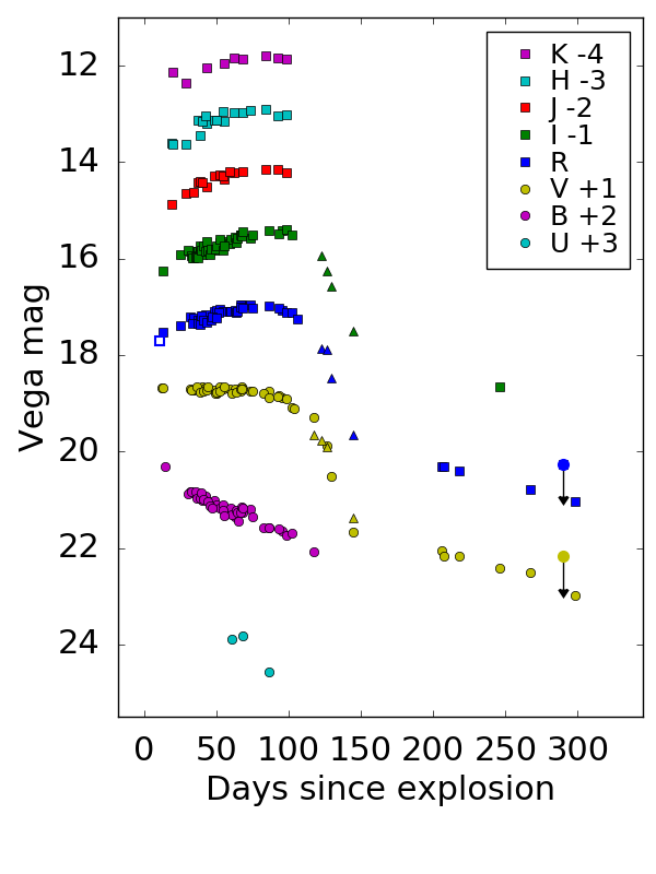
Figure 3: Light curves of SN 2013K in the UBVRIJHK bands. The triangles are gri-band data converted to the Johnson-Cousins system (VRI) using transformation formulas from Chonis & Gaskell (2008). The empty square point on the $R$-band light curve is the unfiltered discovery magnitude from Taddia et al. (2013).

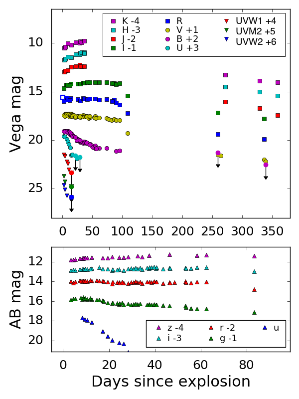
Figure 4: Multiband UV and optical light curve of SN 2013am. The Swift UVW1, UVM2, UVW2 bands are also included. The empty square point on the $R$-band light curve is the unfiltered discovery magnitude from Nakano et al. (2013).

4.2 Extinction

In order to determine the intrinsic properties of the SN, a reliable estimate of the total reddening along the line of sight is needed, including the contribution of both the Milky Way and the host galaxy. The values of the foreground Galactic extinction derived from the Schlafly & Finkbeiner (2011) recalibration of the Schlegel, Finkbeiner, & Davis (1998) infrared-based dust map are $E$($B-V$)_MW = 0.022 mag for SN 2013am and $E$($B-V$)_MW = 0.126 mag for SN 2013K. However, a relatively high contribution from the host galaxy is needed to explain the red colour of the spectral continuum, especially for SN 2013am (Benetti et al., 2013).

To estimate the total reddening, we use the relation between the extinction and the equivalent width (EW) of the interstellar Na I D doublet (e.g. Turatto, Benetti, & Cappellaro, 2003; Poznanski, Prochaska, & Bloom, 2012), though we acknowledge that there is a large associated uncertainty due to the intrinsic scatter in this relation. We found that the Na I D absorption features can be detected in both SNe, with resolved host galaxy and Milky Way components. From the medium-resolution (2 Å) spectra of SN 2013am obtained with the ANU 2.3m telescope (+WiFes spectrograph, phase +4.3 d and +7.6 d), we measured the EW($D_{1}+D_{2}$) for the Galactic and host Na I D absorptions to be $\sim$0.24 Å and $\sim$1.40 Å, respectively. Applying the Poznanski, Prochaska, & Bloom (2012) empirical relations (their eq. 9), we obtain $E$($B-V$)_MW = 0.026${}_{-0.004}^{+0.006}$ mag, in excellent agreement to the extinction from Schlafly & Finkbeiner (2011) mentioned above, and $E$($B-V$)_host = 0.63${}_{-0.09}^{+0.13}$ mag. Applying a similar analysis to a lower resolution spectrum of SN 2013K, we find $E$($B-V$)_MW = 0.10${}_{-0.02}^{+0.04}$ mag (also in agreement with the value inferred from the infrared dust map), and a similar extinction inside the host galaxy.

Overall, from the analysis of the Na I D lines we obtain moderate total extinction values, i.e. $E$($B-V$)${}_{tot}\approx 0.65\pm 0.10$ mag for SN 2013am ($A_{V}\approx 2$ mag, using the reddening law of Cardelli et al. 1989), and $E$($B-V$)${}_{tot}\approx 0.25\pm 0.20$ mag for SN 2013K ($A_{V}\approx 0.7$ mag), consistently with the location of the SNe in dusty regions of their host galaxies. These values are adopted in the following analysis.

We find that after applying these reddening corrections to the spectra, the GELATO spectral classification tool (Harutyunyan et al., 2008) gives excellent matches to the low-velocity Type IIP SN 2005cs. We also note that our reddening estimate for SN 2013am is consistent, within the error, with the value derived by Zhang et al. (2014; cf. their Section 3.4).

A consistency check of the adopted extinction values is based on the Nugent et al. (2006) correlation between the absolute magnitude of Type II SNe in $I$ band and the expansion velocity derived from the minimum of the Fe II $\lambda$ 5169 P-Cygni feature observed during the plateau phase, at $t\approx+50$ d (their eq. 1). In Fig. 7 we plot the sample of nearby Type II SNe and the derived relation between absolute magnitude and photospheric velocity from Nugent et al. (2006; cf. their table 4). In this figure, we add the data for five additional events: SNe 2005cs (Pastorello et al., 2009), 2009ib (Takáts et al., 2015), 2012A (Tomasella et al., 2013), 2013K and 2013am (this work). After applying our adopted extinction correction, both SN 2013K and 2013am follow the expected relation.

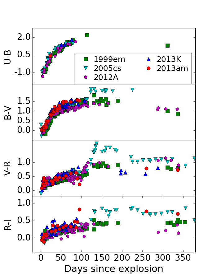
Figure 5: From top to the bottom: $U-B$, $B-V$, $V-R$, $R-I$ colours of SNe 2013am and 2013K from early times to the nebular phase, compared to SNe 2005cs, 2012A and 1999em (see text for a discussion).

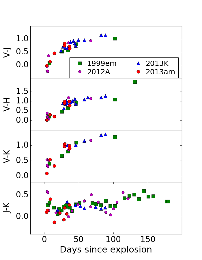
Figure 6: NIR colour evolution of SNe 2013am and 2013K, compared to that of SNe 2012A and 1999em.

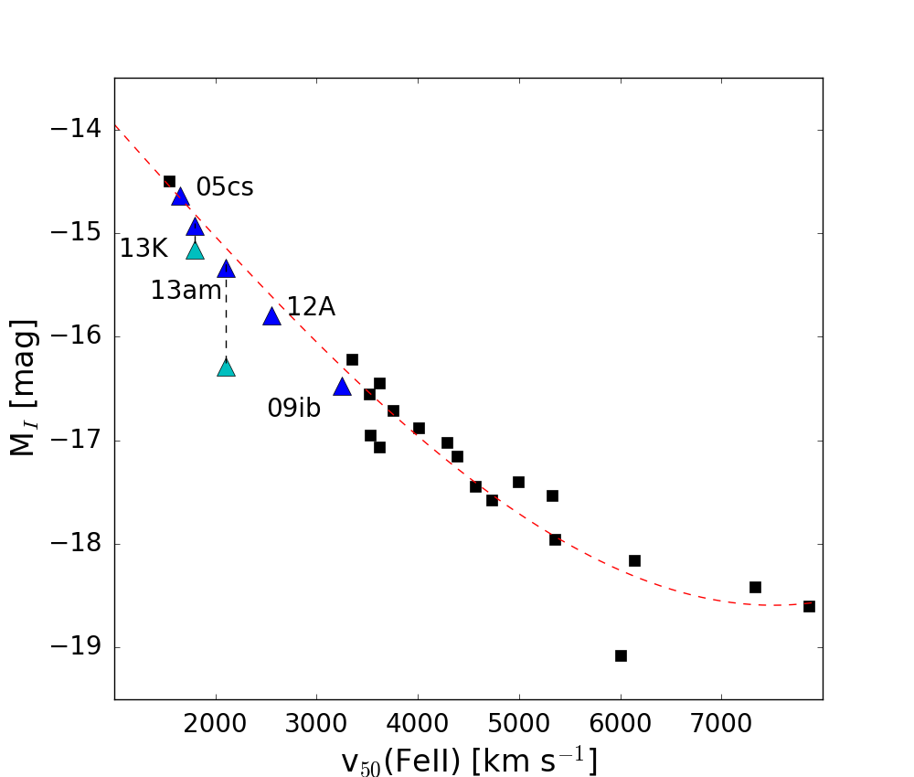
Figure 7: Velocity-luminosity relation for a sample of nearby Type II SNe collected by Nugent et al. 2006 (black squares; their table 4). The fit to the data (dashed red line) is their eq. (1). The blue triangles are SNe 2005cs, 2009ib, and 2012A (Pastorello et al. 2009; Takáts et al. 2015; Tomasella et al. 2013), and SNe 2013K and 2013am (this work). For the latter two SNe, the cyan triangles are before applying the extinction correction.

4.3 Absolute magnitudes

With the above distances (Section 2, Table 1), apparent magnitudes (Section 4.1), and extinctions (Section 4.2), we derive the following peak absolute magnitudes: $M_{V}\sim-15.6\pm 0.2$, $M_{R}=-16.2\pm 0.2$ for SN 2013K; $M_{B}=-16.1\pm 0.2$, $M_{V}=-16.2\pm 0.3$ and $M_{R}=-16.4\pm 0.3$ for SN 2013am. The absolute magnitudes of both SNe are intermediate between the faint SN 2005cs ($M_{V}=-15.1\pm 0.3$ mag, cf. Pastorello et al., 2006; Pastorello et al., 2009), and normal Type IIP SNe, that have an average peak magnitude of $M_{V}=-16.74$ mag ($\sigma=1.01$; cf. Anderson et al., 2014, see also Galbany et al. 2016). The brightest normal Type IIP SNe can reach magnitudes around $\sim-18$ mag (Li et al., 2011; Anderson et al., 2014).

4.4 Colour curves

The optical and NIR colour curves of both SNe 2013K and 2013am after correction for the Galactic and host galaxy reddening (cf. Section 4.2) are shown in Figs 5 and 6. For a comparison, we also plot the colour evolution of the normal Type IIP SNe 1999em (Elmhamdi et al., 2003), 2012A (Tomasella et al., 2013), and the faint 2005cs (Pastorello et al., 2009). The common rapid colour evolution, especially in $B-V$, during the first month of evolution is due to the expansion and cooling of the photosphere. Between 100 and 150 days, both SN 2013am and SN 2013K show very little variation, similar to that experienced by the normal Type II SNe 2012A and 1999em, while the faint Type II SNe (e.g. SN 2005cs and SN 2009md, see Pastorello et al., 2009; Spiro et al., 2014; Fraser et al., 2011, and references therein) sometimes show a red peak in colour during the drop from the plateau phase. Contrary to the claim of Zhang et al. (2014; cf. their fig. 5) of an unusual $V-I$ red colour for SN 2013am during the nebular phase, the colour evolution for both SNe 2013am and 2013K is consistent with the normal Type II SNe, with no evidence of the red spike characterising the underluminous SNe 2005cs and 2009md five months after explosion.

4.5 Pseudo-bolometric light curves and ejected Nickel masses

The pseudo-bolometric luminosities of SNe 2013K and 2013am are obtained by integrating the available photometric data from the optical to the NIR. We adopt the following procedure: for all epochs we derived the flux at the effective wavelength in each filter. When observations for a given filter/epoch were not available, the missing values were obtained through interpolations of the light curve or, if necessary, by extrapolation, assuming a constant colour from the closest available epoch. The fluxes, corrected for extinction, provide the spectral energy distribution at each epoch, which is integrated by the trapezoidal rule, assuming zero flux at the integration boundaries. The observed flux is then converted into luminosity, given the adopted distance to each SN. The error, estimated by error propagation, is dominated by the uncertainties on extinction and distance. The UV-optical photometry retrieved from the Swift Data Center is also included when computing the pseudo-bolometric light curve of SN 2013am. Instead, UV measurements are not available for SN 2013K and hence for this object the bolometric luminosity does not include this contribution. At very early phases the far UV emission contributes almost 50 per cent of the total bolometric luminosity, dropping to less than 10 per cent in about two weeks. This has to be taken into account when comparing SN 2013am with SN 2013K. Also, the striking diversity in the first $\sim$20 days of the light curves of Type IIP SNe may be attributed to the presence of a dense circumstellar material (CSM), as recently outlined in Morozova, Piro, & Valenti (2017). Colour corrections were applied to convert ubv Swift magnitudes to the standard Landolt UBV system.

The pseudo-bolometric OIR and UVOIR light curves for SNe 2013K and 2013am respectively, are presented in Fig. 8, along with those of SNe 1999em (OIR; adopting $\mu=29.82\pm 0.15$, $A_{B}^{tot}=0.4$ mag, Elmhamdi et al. 2003), 2005cs (UVOIR; $\mu=29.26\pm 0.33$, $A_{B}^{tot}=0.2$ mag, Pastorello et al. 2009) and 2012A (UVOIR; $\mu=29.96\pm 0.15$, $A_{B}^{tot}=0.15$ mag, Tomasella et al. 2013), which were computed with the same technique, including the Swift/UVOT contribution for SNe 2012A and 2005cs, and using $H_{0}$ = 73 km s^-1 Mpc^-1. In Fig. 8 we also plot the OIR light curve for SN 2013am. The ratio between the UVOIR and OIR pseudo-bolometric luminosities of SN 2013am is around 2 at maximum light and decreases to 1.3 ten days after maximum. This is in agreement with the result obtained by Bersten & Hamuy (2009) and Faran, Nakar, & Poznanski (2018) for SN 1999em. Therefore we can assume that a similar correction should be applied to early phase of SN 2013K.

The early luminosity of SN 2013am matches that of SN 2012A, showing a peak luminosity of $L=1.5^{+0.2}_{-0.2}\times 10^{42}$ erg s^-1 at about 2 days after explosion. We note a monotonic, rapid decline from the beginning of the follow-up campaign until 20 days from explosion. Later on, an almost constant plateau luminosity is reached, lasting about 20 days. In the successive 50 days, the light curve shows a slow monotonic decline, followed by a sudden drop, which marks the end of the hydrogen envelope recombination. The latter phase was not monitored as SN 2013am had disappeared behind the Sun. We recovered the SN at very late phases (starting from +261 d), in the linear tail phase, with decline rate close to that expected from the ⁵⁶Co decay. The pseudo-bolometric peak of SN 2013K is reached close to the $R$-band maximum, and shortly before the drop from the plateau, with a luminosity of $L=5.2^{+2.5}_{-1.6}\times 10^{41}$ erg s^-1, however, the missing contribution in the UV can represents a significant fraction of the total flux (up to a factor two), in the early days. The plateau duration and the subsequent drop to the radioactive tail are similar in both SN 2013K and SN 2013am.

The luminosities during the radioactive tails of SNe 2013K and 2013am are comparable to those of SNe 2012A and 1999em, and significantly higher than that of the faint Type IIP SN 2005cs. Comparing the bolometric luminosities of SNe 2013K and 2013am with SN 1987A (from $+280$ to $+340$ d), we obtain a best fit for $L$(13K)$/L$(87A) $=0.18\pm 0.08$ and $L$(13am)$/L$(87A) = $0.20\pm 0.03$. Thus, taking as reference the estimate of the ⁵⁶Ni mass for SN 1987A ($0.075\pm 0.005$ M_⊙, Danziger, 1988; Woosley, Hartmann, & Pinto, 1989), and propagating the errors, we obtain ejected ⁵⁶Ni masses of $0.012\pm 0.010$ and $0.015\pm 0.006$ M_⊙ for SN 2013K and SN 2013am, respectively. Both these values are lower than the typical amount of ⁵⁶Ni ejected by SNe IIP ($\sim 0.06-0.12$ M_⊙, Sollerman 2002, Müller et al. 2017; see also the distribution of ⁵⁶Ni masses of Type II SNe sample by Anderson et al. 2014, showing a mean value of 0.033 M$\odot$ with $\sigma=0.024$). However, these ejected ⁵⁶Ni masses are higher than those associated with Ni-poor ($\lesssim 10^{-2}$ M_⊙), low-energy events such as SNe 1997D (Turatto et al., 1998; Benetti et al., 2001), 2005cs (Pastorello et al., 2006; Pastorello et al., 2009) and other faint SNe IIP (cf. Pastorello et al., 2004; Spiro et al., 2014).

Figure 8: Comparison of the OIR or/and UVOIR pseudo-bolometric light curves of SNe 2013K and 2013am with the low-luminosity SN 2005cs and the normal SNe 1999em and 2012A (see the figure legend and Section 4.5 for details). Some of the discrepancies between the curves of normal SNe 2013K, 2013am and 1999em at early times can be attributed to missing UV flux in the pseudo-bolometric curves. The dashed line indicates the slope of the ⁵⁶Co decay.

4.6 Optical spectra: from photospheric to nebular phases

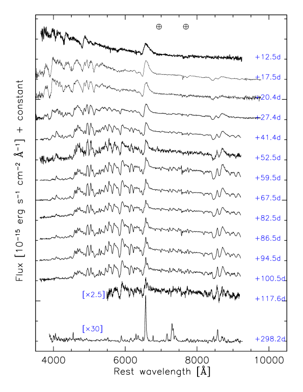
Figure 9: SN 2013K: optical spectral evolution from the photospheric phase (+12.5 d), to the nebular phase (+298.2 d). The spectra have been corrected for reddening and redshift, and shifted vertically for display. Phases (reported on the right of each spectrum) are relative to the explosion date, MJD = 56302.0${}^{+5}_{-5}$. The positions of major telluric features (O₂ A $\&$ B) are marked with $\oplus$ symbols.

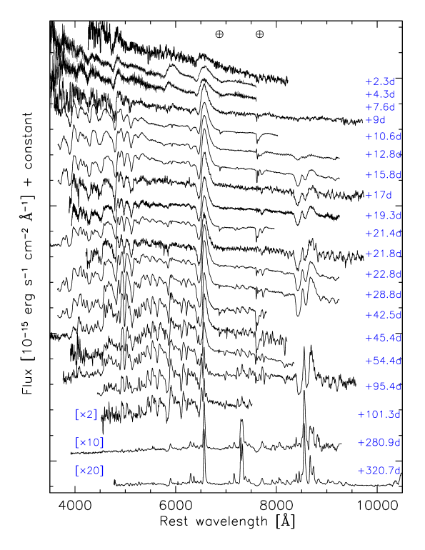
Figure 10: SN 2013am: optical spectral evolution from the very early photospheric (+2.3 d), to the nebular phase (+280.9 d and +320.7 d spectra). Only high signal-to-noise spectra are plotted here. The spectra have been corrected for reddening and redshift, and shifted vertically for clarity. Phases (reported on the right of each spectrum) are relative to the explosion date, MJD = 56371.5${}^{+1.5}_{-1.0}$. Some spectra obtained at nearly the same epoch have been averaged in order to increase the signal-to-noise (e.g. the spectrum at phase +9 d is the average of three spectra taken at +7.8 d, +8.8 d, +9.8 d; the spectrum at phase +17 d is the average of spectra taken in two consecutive nights, +16.8 d and +17.8 d). The positions of major telluric features (O₂ A $\&$ B) are marked with $\oplus$ symbols.

In Figs 9 and 10, we present the entire spectral evolution of SNe 2013K and 2013am, from the photospheric to the nebular phases. For SN 2013am, the spectroscopic follow-up started shortly after the shock breakout. A total of 26 optical spectra were taken, covering phases from $+$2.3 d to $+$320.7 d after the explosion. SN 2013K was caught about 12 days after explosion, and twelve spectra were collected, up until phase +298.2 d. The earlier spectra of both SNe are characterised by a blue continuum and prominent hydrogen Balmer lines with broad P-Cygni profiles.

4.6.1 Key spectral features

Besides the hydrogen Balmer series, the first spectrum of SN 2013am (+2.3 d) shows a broad-line feature just blueward of H${\beta}$ which is tentatively associated with He II $\lambda$ 4696 (the presence of this line in Type IIP SNe 1999gi and 2006bp is extensively discussed by Dessart et al., 2008). Two days later, He I $\lambda$ 5876 emerges. At this phase (+4.3 d), it is comparable in strength to H${\alpha}$, before weakening (+7.6 d) and disappearing soon after (+9 d). The first spectrum of SN 2013K, taken at phase +12.5 d, displays only a hint of He I $\lambda$ 5876.

A few weeks later, the dominant features in both SNe 2013K and 2013am are metal lines with well developed, narrow P-Cygni profiles, arising from Fe II ($\lambda$ 4500, $\lambda\lambda\lambda$ 4924, 5018, 5169, multiplet 42; these lines are also present in earlier spectra), Sc II ($\lambda$ 4670, $\lambda$ 5031), Ba II ($\lambda$ 4554, $\lambda$ 6142), Ca II ($\lambda\lambda\lambda$ 8498, 8542, 8662, multiplet 2, and H&K), Ti II (in a blend with Ca II H&K), and Na I D (close to the position of the He I $\lambda$ 5876). The permitted lines of singly ionised atoms of Fe and Ba begin to appear at phase $+$10.6 d for SN 2013am, and slightly later ($+$17 d) for SN 2013K. As the SNe evolve, their luminosity decreases, and their continua become progressively redder and dominated by metallic lines, such as Na I D and Ca II IR triplet. These features are clearly visible about one month after the explosion. In both SNe, strong line blanketing, especially due to Fe II transitions, suppresses most of the UV flux below 4000 Å.

4.6.2 Photospheric temperature

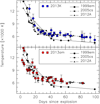
Figure 11: Evolution of the continuum temperature of SNe 2013K (top panel) and 2013am (bottom panel), and comparison with SNe 1999em, 2012A and the faint SN 2005cs. For SNe  2013K and 2013am, the blue and red squares are derived by fitting a black-body to the photometric data, while blue and red circles by fitting a black-body to spectra.

Estimates of the photospheric temperatures are derived from black-body fitting of the spectral continuum (the spectra are corrected for the redshift and adopted extinctions), from a few days after explosion up to around two months (using the iraf/stsdas task nfit1d). Later on the fitting to the continuum becomes difficult, due to both emerging emission lines and increased line blanketing by iron group elements (Kasen & Woosley, 2009) which causes a flux deficit at the shorter wavelengths. Actually, when the temperature drops below $10^{4}$ K, the UV flux is already suppressed by line blanketing, and the effect becomes even stronger on the blue bands as the temperature decreases down to $\sim 8000$ K (Faran, Nakar, & Poznanski, 2018, cf. their Section 3 and Fig. 1). Consequently, the black-body fitting to the spectral continuum is performed using the full wavelength range (typically 3350-10000 Å) solely during the first ten days of evolution. At a later time, wavelengths shorter than 5000 Å are excluded from the fit because the blanketing affects also the B-band. We note that estimating the temperature is very challenging, both at early phases, when the peak of the spectral energy distribution is blueward of 3000 Å, i.e. outside our spectral coverage, and at late phases, due to the numerous emission and absorption lines. Setting the sample range of the black-body fitting in order to include or exclude the stronger emission or absorption features, we quantify that the typical uncertainty for the temperature determination is greater than $\sim 500$ K.

Also, we estimate the photospheric temperatures by fitting a black-body to the available multi-band photometry (Section 4.1). Following Faran, Nakar, & Poznanski (2018), we exclude from the fitting the bluest bands when the effect of line blanketing on the SED is appreciable. The uncertainties on the inferred values are estimated with a bootstrap resampling technique, varying randomly the flux of each photometric point according to a normal distribution having variance equal to the statistical error of each point. We do this procedure 1000 times for each epoch, measuring a temperature from each resampling. The error of the temperature is the standard deviations of the new inferred distribution.

The temperature evolution of SNe 2013K and 2013am is shown in Fig. 11, along with SNe 2012A, 1999em and 2005cs, for comparison. Data obtained by fitting a black-body to the spectra and to the SED are marked with different symbols (circles and squares, respectively), along with the error of the fit. As pointed out by Faran, Nakar, & Poznanski (2018), at early phases, the Swift UV photometry (available only for SN 2013am) is critical for constraining the black-body fit to the SED, causing differences as large as $\sim 2500$ K from the one derived by fitting the coeval spectrum, which covers only wavelengths redward of the U-band. After phase +20 d, the deviation is within the error bars. For both SNe 2013K and 2013am, the early photospheric temperature is above $1.2\times 10^{4}$ K and decreases to $\sim 6000$ K within two months, at the end of the plateau phase.

4.6.3 Expansion velocity

From each spectrum of SNe 2013K and 2013am, we measure the H${\alpha}$ and H${\beta}$ velocity and, where feasible, the Fe II $\lambda$ 5169, Sc II $\lambda$ 5527 and Sc II $\lambda$ 6246. This is done by fitting Gaussian profile to the absorption trough in the redshift corrected spectra. Following Leonard et al. (2002), the error estimate includes the uncertainty in the wavelength scale and in the measurement process itself. The wavelength calibration of spectra is checked against stronger night-sky lines using the cross-correlation technique (O I, Hg I and Na I D, Osterbrock et al. 2000), thus assigning an 1$\sigma$ error of $\sim$ 0.5 Å. To evaluate the fit error, we normalise the absorption feature using the interpolated local continuum fit and we perform multiple measurements adopting different choices for the continuum definition. The standard deviation of the measures is added in quadrature to the uncertainty of the wavelength scale, giving a total, statistical (not systematic) uncertainty for the velocity of each line ranging from 50 to 200 km s^-1 (depending on the signal-to-noise ratio of each spectrum and on the strength of the measured feature).

As discussed by Dessart & Hillier (2005), the velocity measured at the absorption minimum, v_abs, can overestimate or underestimate the photospheric velocity, $v_{phot}$, especially when considering Balmer absorptions. However, for the Fe II $\lambda$ 5169 line, the velocity measurement $v_{abs}$ matches $v_{phot}$ to within 5-10% (see Dessart & Hillier, 2005, their Fig. 14), and also, the Sc II $\lambda$ 6246 line is considered a good indicator of the photospheric velocity $v_{phot}$ (Maguire et al., 2010).

In Fig. 12 we plot the H${\alpha}$, H${\beta}$ velocity $v_{abs}$, for SN 2013K (top panel) and SN 2013am (middle panel) during the first two weeks of evolution, while the Fe II and Sc II features are identified and measured only at later phases. In the bottom panel of Fig. 12 we compare $v_{abs}\approx v_{phot}$ of SNe 2013K and 2013am as derived from the Sc II $\lambda$ 6246 line with those of SNe 1999em, 2012A, 2009N and 2005cs. At early phases, we consider the H$\beta$ velocity as a proxy to Fe II $\lambda$ 5169, applying the linear correlation derived by Poznanski, Nugent, & Filippenko (2010), i.e. $v_{FeII}=0.84\pm 0.05$ $v_{H\beta}$, and plotting these data as open (blue) triangles and (red) circles, respectively. At phase $\sim 95$ d, the velocity settles around 1500 km s^-1 for both SNe 2013K and 2013am.

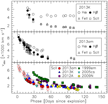
Figure 12: Top panel: evolution of the velocity measured from H$\alpha$, H$\beta$, Fe II $\lambda$ 5169 and Sc II $\lambda$ 6246 in SN 2013K and (middle panel) for SN 2013am. The statistical uncertainty in the velocity estimates (maximum 200 km s^-1) is smaller than the plotted points. Bottom panel: evolution of the velocity of Sc II $\lambda$ 6246 for SNe 2013K, 2013am, 1999em, 2012A, 2009N and 2005cs. The open (blue) triangles and (red) circles are derived in earlier phases from the absorption minima of H$\beta$ for SN 2013K and 2013am, respectively, applying the linear correlation between H$\beta$ and Fe II velocities determined by Poznanski et al. 2010. In this case, an additional error of about 300 km s^-1 is considered and plotted.

4.6.4 Nebular spectra

In Fig. 13 we compare the nebular spectra of SNe 2013K and 2013am, taken around 1 year after explosion, with the standard Type IIP SN 1999em (Elmhamdi et al., 2003), the faint SN 2005cs (Pastorello et al., 2009) and the intermediate-luminosity SN 2009N (Takáts et al., 2014). The narrow H${\alpha}$ emission lines have FWHM (corrected for the instrumental resolution) of about $27\pm 2$ Å for SN 2013am and $23\pm 3$ Å for SN 2013K, corresponding to velocities of $\sim 1200$ and $\sim 1000$ km s^-1, respectively. Maguire et al. 2012 (see their Sections 4.1 and 7) derived an empirical relation between the mass of ⁵⁶Ni and the corrected FWHM of H$\alpha$ for a sample of seven SNe, from the underluminous SN 1997D to SN 1987A. Including SNe 2013am, 2013K (cf. Section 4.5) and SN 2012A (FWHM = $40\pm 2$ Å , M(⁵⁶Ni) = 0.011 M_⊙, see Tomasella et al., 2013), we double the sample size in the sub-energetic tail. Additionally, we include the intermediate-luminosity SN 2009ib (FWHM = $50\pm 2$ Å , M(⁵⁶Ni) = 0.046 M_⊙, see Takáts et al., 2015) with moderate expansion velocities, as already done for Fig. 7. The updated plot of FHWM versus ejected ⁵⁶Ni mass is shown in Fig. 14. We performed a linear least squares fit to the data, weighting each point by its uncertainties, and find that

$$\mathrm{M}(^{56}\mathrm{Ni})=(1.25\pm 0.23)\times 10^{(-0.024\pm 0.009)\times\mathrm{FWHM}}\times 10^{-3}\mathrm{M}_{\odot}$$ (1)

with $\sigma=0.009\pm 0.012$. Pearson’s correlation coefficient and Spearman’s rank correlation are 0.921 and 0.909, respectively.

Figure 13: Top panel: comparison between nebular spectra, obtained about 1 yr after explosion, of SN 2013am and SN 2005cs, and lines identification. Bottom panel: nebular spectra of SN 2013K, SN 1999em and SN 2009N. The inset on top left corner shows a closed up view of the SN 2013am spectrum centred on [Ca II] $\lambda\lambda$ 7291, 7323; the positions of [Fe II] $\lambda$ 7155, [Fe II] $\lambda$ 7172, [Fe II] $\lambda$ 7388, [Fe II] $\lambda$ 7453, [Ni II] $\lambda$ 7378 and [Ni II] $\lambda$ 7412 are also marked. The inset on top right corner shows the [O I] $\lambda\lambda$ 6300, 6364 doublet for SN 2013am at +320.7 d (solid line), compared with the spectrum at phase +280.9 d (dotted line).

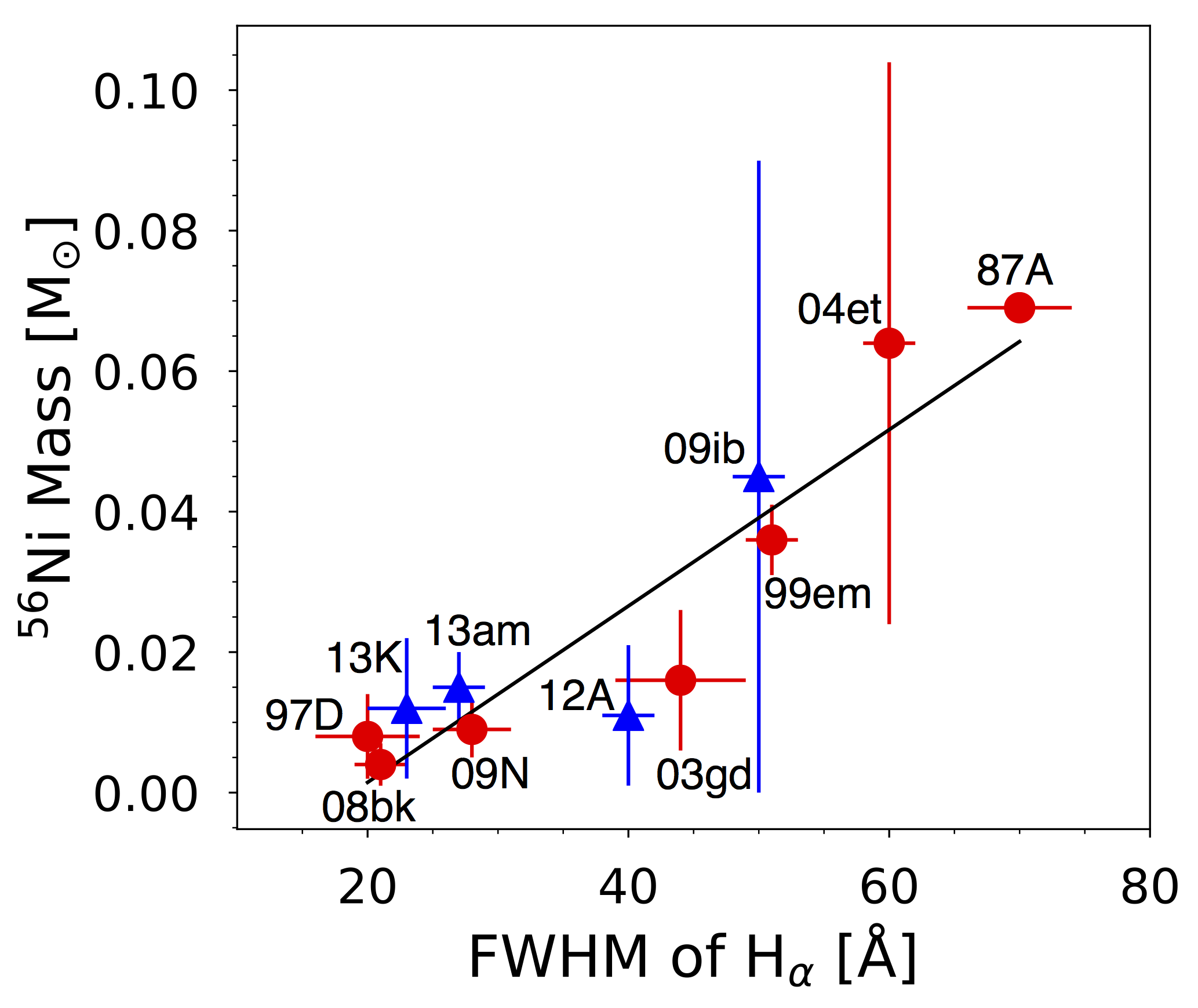
Figure 14: Correlation between the FWHM of H${\alpha}$ (corrected for instrumental resolution) obtained from nebular spectra of a sample of well studied SNe and the ejected mass of ⁵⁶Ni obtained from the nebular tail of their light curves (new data for SNe 2009ib, 2012A, 2013K and 2013am are plotted as blue triangles). See text for details of the derived weighted least squares fit to the data.

The Na I D (still showing residual P-Cygni absorption) and Ca II NIR triplet lines are well detected. The feature at around 7300 Å that is always observed in the nebular spectra of Type IIP SNe, is identified as the [Ca II] $\lambda\lambda$ 7392, 7324 doublet. The individual components of the [Ca II] doublet are resolved. In the last spectrum of SN 2013am, the H${\alpha}$ and [Ca II] doublet have comparable luminosities, resembling the faint SN 2005cs (cf. Fig. 13) rather than normal or intermediate-luminosity Type IIP SNe. In both SNe 2013K and 2013am, the [O I] $\lambda\lambda$ 6300, 6364 doublet is clearly detected, though much weaker than [Ca II]. Several lines of [Fe II] (multiplets 19 and 14, with the contribution of multiplet 30, cf. Benetti et al., 2001) are visible in the nebular spectra, along with other weaker features that can be attributed to [Fe I], Fe I, Fe II, O I and Ba II. The latter is clearly identified as the 6497 Å line blueward of H${\alpha}$. Ba II $\lambda\lambda$ 5854, 6497 (the first component is blended with Na I D) together with Ba II $\lambda$ 6142 (blended with Fe I, Fe II) were previously identified in underluminous Type IIP SNe, such as SNe 1997D (Turatto et al., 1998), 2005cs (Pastorello et al., 2009), and 2008bk (Lisakov et al., 2017), but also in the intermediate-luminosity Type IIP SNe 2008in (Roy et al., 2011), 2009N (Takáts et al., 2014) and 1999em (Leonard et al., 2002). The appearance of relatively strong Ba II lines is likely due to the combination of a low temperature (below $\sim$ 6000 K, see Hatano et al. 1999; Turatto et al. 1998) and low expansion velocity (i.e. narrow, unblended lines are better seen, while in standard SNe II the higher expansion rate at the base of the H-rich envelope causes the contributions of Ba II 6497 Å and H$\alpha$ to merge into a single spectral feature, as discussed by Lisakov et al. 2017). We note the presence in SN 2013am of a feature redward of 7000 Å, which could be identified with He I $\lambda$ 7065, even if it is rarely seen in nebular spectra (detected in SN 2008bk by Maguire et al. 2012) or with another metallic forbidden line. In both SNe, we can identify [C I] $\lambda$ 8727 which is a helium burning ash and a tracer of the O/C zone.

The ratio ($\Re$) between the luminosities of the [Ca II] $\lambda\lambda$ 7392, 7324 and [O I] $\lambda\lambda$ 6300, 6364 doublets appears to be almost constant at late epochs, and has been proposed as a diagnostic for the core mass and, consequently, for the main-sequence mass ($M_{\rm ZAMS}$) of the SN progenitor (cf. Fransson & Chevalier, 1987, 1989; Woosley & Weaver, 1995, see also Jerkstrand et al. 2012). $\Re$ is inversely proportional to the precursor’s $M_{\rm ZAMS}$. From the emission line spectra of the peculiar Type II SN 1987A it was found $\Re\approx 3$ (Li & McCray, 1992, 1993). Extensive studies on the blue progenitor of this event indicate an initial mass in the range of $14-20$ M_⊙, i.e. close to the suggested upper limit of 19 M_⊙ for the progenitor mass of Type IIP SN (Dwarkadas, 2014; Smartt, 2015b, see also the reviews by Arnett et al. 1989; Smartt 2009). On the opposite side, the nebular spectrum of SN 2005cs yields a high value of this luminosity ratio, $\Re\approx 4.2\pm 0.6$ (cf. Pastorello et al., 2009), which is consistent with a small He core and hence a low main-sequence mass for the progenitor, close to the minimum initial mass that can produce a SN, namely 8$\pm 1$ M_⊙ (Smartt, 2009). Indeed, pre-explosion HST imaging revealed a $M_{\rm ZAMS}\sim 7-13$ M_⊙ RSG as the precursor of SN 2005cs (cf. Eldridge, Mattila, & Smartt, 2007, and references within). Late-time HST observations by Maund, Reilly, & Mattila (2014) confirm the progenitor identification of SN 2005cs, and the progenitor mass was refined to $M_{\rm ZAMS}=9.5^{+3.4}_{-2.2}$ M_⊙. In between, we find that the nebular spectrum of SN 1999em plotted in Fig. 13 is characterised by $\Re\approx 3.6\pm 0.5$, suggesting a progenitor of moderate main-sequence mass, in the range of $12-15$ M_⊙. Coherently, for this event $M_{\rm ZAMS}\sim 12\pm 1$ M_⊙ was derived by Smartt et al. (2002), analysing the pre-SN images of the Canada-France-Hawaii Telescope archive, while the hydrodynamical modelling in Elmhamdi et al. (2003) suggested $M_{\rm ZAMS}\sim 12-14$ M_⊙.

Similar to SN 1999em, the line strength ratio from the spectrum of SN 2013am at phase +320.7 d, is $\Re\approx 3.7\pm 0.5$; an analogous value is derived for SN 2013K at $+$298.2 d, although with a larger uncertainty due to the lower signal-to-noise ratio of the spectrum. Again, these intermediate $\Re$ are suggestive of moderate-mass progenitors ($12-15$  M_⊙). The hydrodynamical modelling described in Section 5 supports this hint. We caution however that the line ratio is only a rough diagnostic of the core mass, due to the contribution to the emission from primordial O in the hydrogen zone (Maguire et al., 2012; Jerkstrand et al., 2012). Moreover, mixing makes it difficult to derive relative abundances from line strengths, as discussed in Fransson & Chevalier (1989). An example of these effects can be seen for SN 2012A, were we find $\Re\approx 2$ (cf. Tomasella et al. 2013, their table 8), which would suggest a higher mass than that inferred by Tomasella et al. (2013) either through the direct detection of the progenitor in pre-SN images ($10.5^{+4.5}_{-2}$ M_⊙), or hydrodynamical modelling of the explosion ($14-15$ M_⊙).

4.6.5 Nickel and Iron forbidden lines

SNe 2013K and 2013am show distinct, narrow [Fe II] $\lambda$ 7155 and [Ni II] $\lambda$ 7378 lines in their nebular spectra (fig. 13). The emissivity ratio of [Ni II] to [Fe II] ($L_{7378}/L_{7155}$) is also considered a diagnostic of the Ni to Fe ratio, as discussed by Jerkstrand et al. (2015, 2015a). From a Gaussian fit to these lines, we determine a ratio $\sim 1$ for both the SNe. This implies an abundance number ratio Ni/Fe $\approx 0.06\pm 0.01$, i.e similar to the solar value (Jerkstrand et al., 2015, their Section 5.1.4). According to Jerkstrand et al. (2015a), SNe that produce solar or subsolar Ni/Fe ratios must have burnt and ejected only Oxygen-shell material. On the other hand, a larger Ni/Fe ratio would imply that there was explosive burning and ejection of the silicon layer, as in the case of SNe 2006aj and 2012ec (see Jerkstrand et al. 2015, Maeda et al. 2007 and Mazzali et al. 2007). The solar Ni/Fe ratio measured for both SNe 2013K and 2013am again would suggest medium-mass progenitors, with M_ZAMS of about 15 M_⊙ (cf. Jerkstrand et al. 2015a, their Fig. 8).

4.6.6 Oxygen forbidden lines

Jerkstrand et al. (2012) used their spectral synthesis code to model the nebular emission line fluxes for SN explosions of various progenitors, and find the [O I], Na I D and Mg I] lines to be the most sensitive to ZAMS mass. In particular, the [O I] lines appear to be a reliable mass indicator (see also Chugai, 1994; Chugai & Utrobin, 2000; Kitaura, Janka, & Hillebrandt, 2006). Unfortunately, the nebular spectrum of SN 2013K has a low signal-to-noise ratio, and there appears to be significant contamination from the Fe I $\lambda$ 6361 line (Dessart & Hillier, 2011, see their fig. 17). The [O I] line flux relative to ⁵⁶Co luminosity (assuming M(⁵⁶Ni) = $0.012\pm 0.010$ M_⊙ and a distance of 34 Mpc) is estimated to be of the order of $3-4$ per cent. Based on the modelling of Jerkstrand et al. 2012 (their Fig. 8), this ratio would suggest a moderately massive star, between 15 and 19 M_⊙, as the precursor of SN 2013K. Conversely, from the high signal-to-noise nebular spectrum of SN 2013am taken at phase +320.7 d (assuming M(⁵⁶Ni) = $0.015\pm 0.006$ M_⊙ and a distance of 12.8 Mpc) we find that the [O I] $\lambda\lambda$ 6300, 6364 flux relative to ⁵⁶Co luminosity is only $\sim 0.6$ per cent. The low value seems to point to a progenitor for SN 2013am of less than 12 M_⊙. This is in contrast with other indicators, including the luminosity ratios [Ca II]$/$[O I] and [Ni II]$/$[Fe II] calculated previously, and the hydrodynamical model (cf. Section 5), which indicate for both SNe moderate-mass progenitors, in the range $12-15$ M_⊙.

We caution that the nebular models in Jerkstrand et al. (2012) are computed for a higher ejected ⁵⁶Ni mass (M(⁵⁶Ni) = 0.062 M_⊙, as derived for SN 2004et) and higher velocities of the core material ($\sim 1800$ km s^-1, which is at least 30 per cent larger than the velocities estimated for SNe 2013K and 2013am). Jerkstrand et al. (2015) investigated the sensitivity of line flux ratios by varying the mass of ejected ⁵⁶Ni from 0.06 to 0.03 M_⊙, and concluded that the diagnostics are reliable in this range. However, SNe 2013K and 2013am have much smaller M(⁵⁶Ni). New models for both low-velocity and low M(⁵⁶Ni) Type II SNe are being produced (Jerkstrand et al., in prep.), and detailed comparison of the new models with the spectra of SNe 2013K and 2013am and other Type II SNe will be included in this work.

Simulations of stellar collapse and low energy explosions performed by Kitaura, Janka, & Hillebrandt (2006) point to a clear difference between low-mass and more massive SN progenitors. The former, like SN 1997D (Chugai & Utrobin 2000), eject a very small amount of O (only a few $10^{-3}$ M_⊙), whereas the latter produce up to a solar mass or more (in the range $1.5-2$ M_⊙ for SN 1987A, see Chugai, 1994). Rescaling the luminosity of [O I] doublet and the M(⁵⁶Ni) to SN 1987A, as done by Elmhamdi et al. (2003) for SN 1999em (their Section 3 and eq. 1), a very rough estimate of the ejected O mass in SN 2013am is $\sim 0.1-0.2$ M_⊙.

Finally, the [O I] $\lambda\lambda$ 6300, 6364 line flux ratio can also be used to determine the optical depth of those transitions (Spyromilio & Pinto, 1991; Spyromilio, 1991; Spyromilio et al., 1991; Li & McCray, 1992), and to calculate the number density of neutral Oxygen in the ejecta. The flux ratio $F_{6364}/F_{6300}$ is around unity in the optically thick limit. As the SN ejecta expand, the ratio decreases to about $1/3$ in the optically thin limit. For SN 2013am, we find $F_{6364}/F_{6300}\approx 0.65$ at phase +280.9 d, decreasing to $\approx 0.56$ at phase +320.7 d, marking the incomplete transition from the optically thick towards the optically thin case. This is similar to what was found for a sample of Type IIP SNe by Maguire et al. (2012; cf. their Section 5.4 and fig. 12). Following Spyromilio et al. (1991), it is possible to uniquely determine the number density of neutral O with only one observation between the optically thick and optically thin limits. For SN 2013am, we derive a neutral O number density of about $\sim 1.0\pm 0.5\times 10^{9}$ cm^-3.

4.7 Infrared spectra

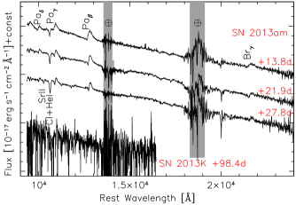
Figure 15: Sequence of NIR spectra of SN 2013am taken with ESO NTT$+$SOFI at phases +13.8, +21.9, +27.8 d (top), shown along with the spectrum of SN 2013K at +98.4 d (bottom). Paschen series, Br${\gamma}$, the blend of C I $\lambda$ 10691 and He I $\lambda$ 10830, and Sr II $\lambda$ 10327 lines are identified. The positions of major telluric features are marked with $\oplus$ symbols.

NIR spectra were collected for SN 2013am (three epochs) and SN 2013K (one epoch) during the photospheric phase with NTT$+$SOFI (cf. Tables 11 and 12). They are plotted in Fig. 15. The Paschen series (with the exclusion of Pa${\alpha}$, which is contaminated by a strong telluric band), Br${\gamma}$, the blend of C I $\lambda$ 10691 and He I $\lambda$ 10830, and Sr II $\lambda$ 10327 are identified. In the spectra of SN 2013am, a relatively strong feature redward of Pa${\gamma}$ can be identified as the O I $\lambda$ 11290 Bowen resonance fluorescence line (Pozzo et al., 2006).

For SN 2013am, the expansion velocity of ejecta, as measured from the absorption minima of Pa${\beta}$ and Pa${\gamma}$, is $\sim 5100$ km s^-1 at phase +13.8 d, decreasing to $\sim 3400$ km s^-1 (+21.9 d) and $\sim 2500$ km s^-1 after one month of evolution. As expected, this expansion velocity is lower than that obtained at similar epochs from the Balmer lines. Rather, it is comparable to the values obtained from the metal lines in the optical spectra (cf. Fig. 12). After smoothing the noisy NIR spectrum of SN 2013K at phase $+98.4$ d, an expansion velocity from Pa${\gamma}$ of about $\sim 2500-3000$ km s^-1 is found, which lies in between the velocities derived from the H${\alpha}$ absorption minimum and Sc II $\lambda$ 6246 at the same epoch.

5 Hydrodynamical modelling

The physical properties of the SN 2013K and SN 2013am progenitors at the time of the explosion, namely the ejected mass ($M_{ej}$), the initial radius ($R$), and the total explosion energy ($E$), are derived from the main observables (i.e. the pseudo-bolometric light curve, the evolution of line velocities and the photospheric temperature), using a well-tested radiation-hydrodynamical modelling procedure. A complete description of this procedure is available in Pumo et al. (2017). To obtain the best fit, a two step procedure is adopted using two different codes: 1) a semi-analytic code (Zampieri et al., 2003), which solves the energy balance equation for ejecta of constant density in homologous expansion; and 2) a general-relativistic, radiation-hydrodynamics Lagrangian code (Pumo, Zampieri, & Turatto, 2010; Pumo & Zampieri, 2011), which was specifically tailored to simulate the evolution of the physical properties of the SN ejecta and the behaviour of the main SN observables up to the nebular stage, taking into account both the gravitational effects of the compact remnant and the heating due to the decay of radioactive isotopes synthesised during the explosion. The former code is used for a preliminary analysis aimed at constraining the parameter space describing the SN progenitor at the time of the explosion and, consequently, to guide more realistic, but time consuming simulations performed with the latter code.

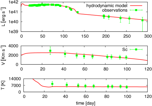
Figure 16: Comparison of the evolution of the main observables of SN 2013K with the best-fit model computed with the general-relativistic, radiation-hydrodynamics code. The best-fit model parameters are: $E=0.34\pm 0.10$ foe, $R=3.2\pm 0.5\times 10^{13}$ cm, $M_{ej}=12.0\pm 1.8$ M_⊙. Top, middle, and bottom panels show the bolometric light curve, the photospheric velocity, and the photospheric temperature as a function of time. To estimate the photospheric velocity from the observations, we use the minima of the profile of the Sc II lines.

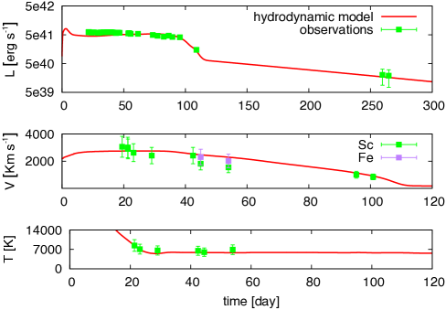
Figure 17: Same as Fig. 16, but for SN 2013am. The best-fit model parameters are: $E=0.40\pm 0.12$ foe, $R=2.5\pm 0.4\times 10^{13}$ cm, $M_{ej}=11.5\pm 1.7$ M_⊙. In the middle panel, Fe II velocity at phase $+45.4$ and $+54.4$ d is also plotted, as comparison.

Adopting the explosion epochs of Section 2, and the bolometric luminosities and M(⁵⁶Ni) as in Section 4.5, we compute the best-fitting models, shown in Figs 16 and 17, for SNe 2013K and 2013am, respectively. We note the general agreement, within the errors, of the best-fitting models with the observables, unless for the Sc II line velocities of SN 2013am at phase $+45.4$ and $+54.4$ d; instead, at these two epochs, the model fit well the velocity of Fe II (cf. Figure 17, middle panel).

The best-fit model of SN 2013K has $E=0.34$ foe, $R=3.2\times 10^{13}$ cm ($\sim 460$ R_⊙), and $M_{ej}=12$ M_⊙. Adding the mass of the compact remnant ($\sim 1.3-2$ M_⊙) to that of the ejected material, we obtain a total stellar mass of $\sim 13.3-14$ M_⊙ at the point of explosion. Concerning SN 2013am, the best-fit model has $E=0.40$ foe, $R=2.5\times 10^{13}$ cm ($\sim 360$ R_⊙), and $M_{ej}=11.5$ M_⊙, resulting in a total stellar mass of $\sim 12.8-13.5$ M_⊙ at explosion. We estimate that the typical error due to the $\chi^{2}$ fitting procedure is about $15$ per cent for $M_{ej}$ and $R$, and $30$ per cent for $E$. These errors are the $2\sigma$ confidence intervals for one parameter based on the $\chi^{2}$ distributions produced by the semi-analytical models. For both SNe 2013K and 2013am, the outcomes of modelling are consistent with low-energy explosions of moderate-mass red supergiant stars.

6 Summary and further comments

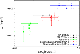
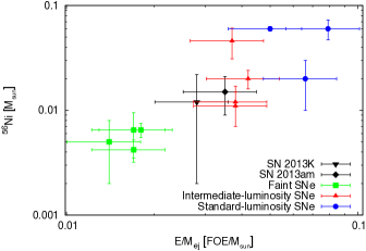
Figure 18: Correlations between the plateau luminosity (top) and ⁵⁶Ni mass (bottom) with the $E/M_{ej}$ ratio, as in Pumo et al. 2017 (their table 2, figs 5, 6), including SNe 2013K and 2013am (black symbols). Like in Pumo et al. 2017 (to which we refers for details), the errorbars on the $E/M_{ej}$ ratios are estimated by propagating the uncertainties on $E$ and $M_{ej}$, adopting a value of 30% for the relative errors of $E$ and 15% for that of $M_{ej}$.

We collected optical and NIR observations of SNe 2013K and 2013am. From the photospheric to the nebular phases, the spectra of these events show narrow features, indicating low expansion velocities ($\sim 1000-1500$ km s^-1 at the end of the plateau), as found in the sub-luminous SN 2005cs. In the photospheric phase, we identify features arising from Ba II, which are typically seen in the spectra of faint Type IIP SNe. Futhermore, the emission line ratios in the nebular spectra of SN 2013am resemble those of SN 2005cs. The NIR spectra show the Paschen and Bracket series, along with He I, Sr II, C I and Mg I features, typical of SNe IIP.

The bolometric luminosities of SNe 2013K and 2013am ($\sim 1.5\times 10^{41}$ erg s^-1 at the plateau), are intermediate between those of the underluminous and normal Type IIP SNe. Indeed, the ejected mass of ⁵⁶Ni estimated from the radioactive tail of the bolometric light curves, is $0.012\pm 0.010$ and $\sim 0.015\pm 0.006$ M_⊙ for SN 2013K and SN 2013am respectively: twice the amount synthesised by the faint SNe 1997D or 2005cs, but 3 to 10 times less than that produced by normal SNe IIP events. Similar ejected ⁵⁶Ni masses were derived for SNe 2012A, 2008in and 2009N (Tomasella et al., 2013; Roy et al., 2011; Takáts et al., 2014).

We used radiation-hydrodynamics modelling of observables (Pumo & Zampieri, 2011) to derive the physical properties of the progenitors at the point of explosion for SNe 2013K and 2013am, finding $M_{ej}$ ($12\pm 1.8$ M_⊙vs. $11.5\pm 1.7$ M_⊙, respectively), $R$ ($3.2\pm 0.5\times 10^{13}$ cm vs. $2.5\pm 0.4\times 10^{13}$ cm), and $E$ ($0.34\pm 0.10$ foe vs. $0.40\pm 0.12$ foe). The inferred parameters are fully consistent with low-energy explosions of medium-mass red supergiant stars, in the range $12.8-14$ M_⊙. With no deep pre-explosion images available for either of these two SNe, the direct detection of their progenitors was not possible. However, the nebular spectra obtained for both SNe were used to constrain the progenitors’ mass. Following Fransson & Chevalier (1989), the luminosity ratio between the [Ca II] $\lambda\lambda$ 7392, 7324 and [O I] $\lambda\lambda$ 6300, 6364 doublets measured at late epochs ($\Re\approx 3.7$, for both SNe) favours red supergiants of moderate mass, between $12-15$ M_⊙. The same progenitor mass range is obtained using the emissivity ratio of [Ni II] $\lambda$ 7378 to [Fe II] $\lambda$ 7155 (Jerkstrand et al., 2015). Instead, comparison to models of nebular spectra calculated by Jerkstrand et al. (2012) for SN 2004et would indicate a lower mass ($\lesssim 12$ M_⊙) and an higher mass ($\gtrsim 15$ M_⊙) progenitor for SN 2013am and SN 2013K, respectively, i.e. outside the mass range favoured by hydrodynamical modelling. However, we stress that specific models for low-velocity, Ni-poor Type IIP SNe are still required (Jerkstrand et al., in preparation).

The physical properties of the progenitors of SNe 2013K and 2013am, as obtained through hydrodynamical modelling, are compared with the ejected M(⁵⁶Ni) and the plateau luminosity at 50 d (L₅₀) in Fig. 18. When compared with the sample of well-studied SNe collected in Pumo et al. (2017), it It appears that the two events bridge the underluminous tail of Type IIP SNe to typical, standard-luminosity events. While the total explosion energy of SN 2013am is similar to that of normal Type IIP SN 1999em (in the range $0.5-1$ foe, see Elmhamdi et al., 2003, and references within), SN 2013K has a lower explosion energy, albiet still comparable to normal Type IIP events (for example SN 2013ab, with 0.35 foe, see Bose et al., 2015). Pumo et al. (2017) suggests that the main parameter controlling where a SN lies within the heterogeneous Type IIP SN class, from underluminous to standard events, is the ratio $E/M_{ej}$. SNe 2013K and 2013am form a monotonic sequence with the other SNe in Fig. 18, indicating, once again, the presence of a continuous distribution from faint, low-velocity, Ni-poor events to bright, high-velocity, Ni-rich objects.

7 Acknowledgments

This work is based (in part) on observations collected at the European Organisation for Astronomical Research in the Southern Hemisphere, Chile as part of PESSTO, (the Public ESO Spectroscopic Survey for Transient Objects Survey) ESO program 188.D-3003, 191.D-0935, 197.D-1075.

This paper is also based on observations collected at: the Copernico 1.82m and Schmidt 67/92 Telescopes operated by INAF Osservatorio Astronomico di Padova at Asiago, Italy; the Galileo 1.22m Telescope operated by Department of Physics and Astronomy of the University of Padova at Asiago, Italy; the Nordic Optical Telescope, operated by The Nordic Optical Telescope Scientific Association at the Observatorio del Roque de los Muchachos, La Palma, Spain, of the Instituto de Astrofisica de Canarias; the Liverpool Telescope operated on the island of La Palma, Spain, by Liverpool John Moores University in the Spanish Observatorio del Roque de los Muchachos of the Instituto de Astrofisica de Canarias with financial support from the UK Science and Technology Facilities Council; the Gran Telescopio Canarias (GTC), installed in the Spanish Observatorio del Roque de los Muchachos in the island of La Palma of the Instituto de Astrofisica de Canarias, Spain; the 3.6m Italian Telescopio Nazionale Galileo (TNG) operated by the Fundación Galileo Galilei - INAF on the island of La Palma, Spain; the Las Cumbres Observatories (LCO) global network; the NTT 3.6m, Trappist and REM Telescopes operated by European Southern Observatory (ESO) in Chile; the SMARTS and Prompt Telescopes operated by Cerro Tololo Inter-American Observatory (CTIO) in Chile; the Australian National University 2.3-m telescope (ANU) at Siding Spring Observatory in northern New South Wales, Australia.

L.T., S.B., A.P., M.T. are partially supported by the PRIN-INAF 2014 project Transient Universe: unveiling new types of stellar explosions with PESSTO. M.F. is supported by a Royal Society - Science Foundation Ireland University Research Fellowship. K.M. acknowledges support from the STFC through an Ernest Rutherford Fellowship. S.J.S. acknowledges funding from the European Research Council under the European Union’s Seventh Framework Programme (FP7/2007-2013)/ERC Grant agreement n^o [291222] and STFC grants ST/I001123/1 and ST/L000709/1. L.G. was supported by the US National Science Foundation under Grant AST-1311862. G.P. is supported by Ministry of Economy, Development, and Tourism’s Millennium Science Initiative through grant IC120009, awarded to The Millennium Institute of Astrophysics. C.P.G. acknowledges support from EU/FP7-ERC grant No. [615929]. C.B. gratefully acknowledge the support from the Wenner-Grenn Foundation. F.E.B. acknowledges support from CONICYT-Chile (Basal-CATA PFB-06/2007, FONDECYT Regular 1141218), the Ministry of Economy, Development, and Tourism’s Millennium Science Initiative through grant IC120009, awarded to The Millennium Institute of Astrophysics, MAS. T-W.C. acknowledges the support through the Sofia Kovalevskaja Award to P. Schady from the Alexander von Humboldt Foundation of Germany. We would like to thank CNTAC for the allocation of REM time through proposals CN2013A-FT-12.

We thank Andrea Melandri for useful comments on the manuscript. We also thank the anonymous referee for the thorough review of the paper.

We are grateful to Istituto Nazionale di Fisica Nucleare Laboratori Nazionali del Sud for the use of computer facilities.

The work made use of Swift/UVOT data reduced by P. J. Brown and released in the Swift Optical/Ultraviolet Supernova Archive (SOUSA). SOUSA is supported by NASA’s Astrophysics Data Analysis Program through grant NNX13AF35G. We acknowledge the Weizmann interactive supernova data repository (http://wiserep.weizmann.ac.il).

Table 3: Magnitudes for the local sequence stars in the fields of SNe 2013K and 2013am.

SN 2013K
ID	R.A.	Dec.	$U$	$B$	$V$	$R$	$I$
a	17:37:24.229	$-$85:16:01.56	$-$	17.24 (0.01)	16.56 (0.01)	16.27 (0.02)	15.64 (0.05)
b	17:37:44.118	$-$85:16:39.05	$-$	16.62 (0.01)	15.92 (0.01)	15.59 (0.01)	15.03 (0.03)
c	17:40:03.075	$-$85:17:04.67	$-$	16.49 (0.01)	15.85 (0.01)	15.49 (0.01)	15.09 (0.04)
d	17:41:20.834	$-$85:17:11.66	$-$	15.34 (0.01)	14.66 (0.01)	14.30 (0.01)	13.81 (0.02)
e	17:38:00.727	$-$85:18:49.69	$-$	17.27 (0.01)	16.50 (0.01)	16.13 (0.01)	15.67 (0.02)
f	17:41:32.752	$-$85:19:31.73	$-$	18.03 (0.01)	17.35 (0.01)	16.98 (0.02)	16.47 (0.03)
g	17:38:11.826	$-$85:19:57.82	$-$	18.63 (0.01)	17.82 (0.01)	17.35 (0.01)	16.78 (0.02)
h	17:41:00.886	$-$85:20:40.59	$-$	18.34 (0.03)	17.66 (0.01)	17.32 (0.01)	16.78 (0.02)
i	17:37:42.199	$-$85:20:36.12	$-$	18.72 (0.02)	18.07 (0.01)	17.76 (0.02)	17.23 (0.04)
j	17:41:31.852	$-$85:15:43.37	$-$	14.41 (0.01)	13.41 (0.01)	12.91 (0.03)	12.35 (0.06)
k	17:38:12.844	$-$85:15:34.54	$-$	18.79 (0.01)	18.09 (0.01)	17.73 (0.02)	17.21 (0.02)
l	17:41:03.387	$-$85:16:15.56	$-$	17.42 (0.01)	16.61 (0.01)	16.21 (0.01)	15.70 (0.03)
m	17:37:57.276	$-$85:17:08.56	$-$	18.17 (0.02)	17.45 (0.01)	17.08 (0.01)	16.58 (0.02)
n	17:41:54.244	$-$85:18:18.32	$-$	18.77 (0.01)	18.10 (0.02)	17.73 (0.01)	17.18 (0.03)
o	17:37:22.590	$-$85:18:13.42	$-$	18.33 (0.01)	17.47 (0.01)	17.05 (0.01)	16.46 (0.02)
p	17:41:24.477	$-$85:19:16.19	$-$	18.01 (0.01)	17.22 (0.02)	16.79 (0.02)	16.12 (0.04)
q	17:38:38.263	$-$85:19:52.86	$-$	17.73 (0.01)	16.99 (0.01)	16.59 (0.01)	16.07 (0.01)
r	17:41:32.707	$-$85:21:02.86	$-$	15.99 (0.02)	15.20 (0.01)	14.80 (0.02)	14.14 (0.02)
s	17:38:30.267	$-$85:20:59.03	$-$	16.69 (0.03)	16.20 (0.03)	15.86 (0.03)	15.35 (0.04)
t	17:41:39.802	$-$85:17:31.23	$-$	17.71 (0.01)	16.89 (0.01)	16.43 (0.01)	15.81 (0.02)
u	17:40:44.322	$-$85:17:49.86	$-$	18.36 (0.01)	17.13 (0.01)	16.37 (0.01)	15.61 (0.03)
v	17:36:49.463	$-$85:17:09.99	$-$	17.38 (0.01)	16.65 (0.01)	16.30 (0.01)	15.82 (0.02)
w	17:36:36.302	$-$85:18:35.50	$-$	17.25 (0.02)	16.22 (0.02)	15.69 (0.01)	15.04 (0.03)
x	17:40:12.352	$-$85:15:46.66	$-$	13.90 (0.01)	12.37 (0.01)	11.52 (0.01)	$-$
SN 2013am
ID	R.A.	Dec.	$U$	$B$	$V$	$R$	$I$
a	11:18:53.136	13:05:05.12	18.56 (0.05)	17.46 (0.06)	16.27 (0.04)	15.59 (0.05)	14.97 (0.09)
b	11:18:57.773	13:05:30.36	15.89 (0.03)	15.45 (0.05)	14.59 (0.04)	14.09 (0.04)	13.66 (0.06)
c	11:19:05.728	13:03:28.38	18.19 (0.03)	18.21 (0.04)	17.55 (0.03)	17.16 (0.03)	16.76 (0.06)
d	11:19:00.156	13:05:34.53	19.50 (0.08)	19.60 (0.04)	19.03 (0.04)	18.69 (0.04)	18.33 (0.06)
e	11:18:52.405	13:03:35.20	12.62 (0.03)	14.44 (0.08)	12.79 (0.04)	11.99 (0.02)	11.71 (0.04)
f	11:18:58.230	13:05:54.53	22.12 (0.83)	21.10 (0.11)	19.53 (0.10)	18.30 (0.17)	16.24 (0.34)
g	11:19:00.421	13:02:21.35	20.11 (0.13)	18.91 (0.07)	17.54 (0.04)	16.75 (0.05)	16.06 (0.10)
h	11:18:55.426	13:04:48.63	20.63 (0.28)	19.81 (0.06)	18.84 (0.06)	18.31 (0.05)	17.93 (0.06)
i	11:18:55.756	13:04:04.68	17.15 (0.04)	18.27 (0.04)	17.96 (0.04)	17.88 (0.06)	18.08 (0.09)

Table 4: SN 2013K: Optical photometry in the UBVRI bands. Errors are given in parentheses.

Date	MJD	$U$	$B$	$V$	$R$	$I$	Instrument
20130120	56312.41	$-$	$-$	$-$	17.70	$-$	CBET3391
20130122	56314.32	$-$	$-$	17.69 (0.01)	$-$	$-$	EFOSC2
20130123	56315.25	$-$	$-$	17.69 (0.16)	17.53 (0.30)	17.25 (0.27)	PROMPT
20130124	56316.29	$-$	18.30 (0.21)	$-$	$-$	$-$	kb77
20130204	56327.36	$-$	$-$	$-$	17.38 (0.11)	16.91 (0.10)	kb77
20130209	56332.36	$-$	18.88 (0.11)	$-$	$-$	16.83 (0.43)	kb77
20130211	56334.25	$-$	18.82 (0.06)	17.70 (0.04)	17.21 (0.04)	16.85 (0.09)	ANDICAM-CCD
20130211	56334.35	$-$	18.84 (0.07)	17.72 (0.05)	$-$	16.94 (0.07)	kb77
20130212	56335.36	$-$	$-$	$-$	17.34 (0.06)	16.98 (0.10)	kb77
20130212	56335.36	$-$	$-$	17.73 (0.05)	$-$	$-$	TRAPPISTCAM
20130213	56336.25	$-$	18.86 (0.05)	17.73 (0.04)	17.24 (0.05)	16.98 (0.07)	ANDICAM-CCD
20130214	56337.36	$-$	18.84 (0.07)	$-$	$-$	16.97 (0.07)	kb77
20130215	56338.36	$-$	18.98 (0.08)	17.66 (0.06)	$-$	16.95 (0.08)	kb77
20130216	56339.25	$-$	18.94 (0.03)	17.69 (0.08)	17.27 (0.03)	16.85 (0.08)	ANDICAM-CCD
20130216	56339.36	$-$	$-$	$-$	17.35 (0.05)	16.98 (0.09)	kb77
20130217	56340.36	$-$	18.97 (0.08)	17.76 (0.06)	17.37 (0.04)	16.73 (0.08)	kb77
20130217	56340.38	$-$	18.93 (0.03)	17.72 (0.03)	17.28 (0.04)	16.88 (0.19)	ANDICAM-CCD
20130218	56341.36	$-$	18.86 (0.10)	$-$	17.19 (0.06)	16.83 (0.09)	kb77
20130219	56342.38	$-$	19.01 (0.03)	17.65 (0.02)	17.19 (0.04)	16.91 (0.05)	ANDICAM-CCD
20130220	56343.36	$-$	18.99 (0.09)	17.75 (0.04)	17.29 (0.04)	16.74 (0.08)	kb77
20130221	56344.25	$-$	18.92 (0.03)	17.68 (0.06)	17.16 (0.04)	16.74 (0.08)	ANDICAM-CCD
20130221	56344.36	$-$	$-$	$-$	$-$	16.84 (0.12)	kb77
20130222	56345.36	$-$	$-$	17.73 (0.05)	17.32 (0.06)	16.65 (0.07)	kb77
20130223	56346.36	$-$	19.04 (0.16)	17.66 (0.06)	$-$	16.83 (0.11)	kb77
20130224	56347.36	$-$	19.12 (0.12)	$-$	$-$	16.91 (0.09)	kb77
20130225	56348.36	$-$	$-$	$-$	17.29 (0.09)	16.80 (0.09)	kb77
20130226	56349.36	$-$	19.17 (0.13)	$-$	17.22 (0.11)	$-$	kb77
20130227	56350.25	$-$	19.02 (0.11)	17.72 (0.05)	17.09 (0.07)	16.83 (0.08)	ANDICAM-CCD
20130228	56351.36	$-$	$-$	17.80 (0.07)	$-$	16.80 (0.08)	kb77
20130301	56352.25	$-$	19.10 (0.10)	17.79 (0.09)	17.08 (0.04)	16.98 (0.09)	ANDICAM-CCD
20130301	56352.36	$-$	$-$	17.77 (0.06)	17.23 (0.06)	16.73 (0.08)	kb77
20130302	56353.38	$-$	$-$	$-$	17.12 (0.38)	$-$	TRAPPISTCAM
20130303	56354.25	$-$	19.17 (0.04)	17.66 (0.03)	17.05 (0.03)	16.66 (0.04)	ANDICAM-CCD
20130303	56354.36	$-$	$-$	17.75 (0.07)	$-$	16.61 (0.08)	kb77
20130305	56356.25	$-$	19.11 (0.04)	17.69 (0.03)	17.09 (0.04)	16.64 (0.05)	ANDICAM-CCD
20130305	56356.36	$-$	19.23 (0.11)	$-$	$-$	16.82 (0.13)	kb77
20130306	56357.36	$-$	19.33 (0.14)	17.66 (0.06)	$-$	16.73 (0.10)	kb77
20130310	56361.25	$-$	19.26 (0.03)	17.70 (0.04)	17.10 (0.08)	16.69 (0.11)	ANDICAM-CCD
20130311	56362.25	$-$	19.18 (0.04)	$-$	17.10 (0.04)	16.59 (0.04)	ANDICAM-CCD
20130311	56362.31	20.89 (0.07)	19.31 (0.02)	17.79 (0.03)	$-$	$-$	EFOSC2
20130314	56365.25	$-$	19.36 (0.08)	17.70 (0.09)	17.07 (0.11)	16.56 (0.21)	ANDICAM-CCD
20130314	56365.36	$-$	19.21 (0.15)	17.78 (0.07)	17.11 (0.10)	16.67 (0.14)	kb73
20130315	56366.36	$-$	19.25 (0.11)	$-$	17.10 (0.05)	16.59 (0.08)	kb73
20130316	56367.36	$-$	19.45 (0.21)	$-$	$-$	$-$	kb73
20130317	56368.32	$-$	19.25 (0.12)	17.74 (0.07)	16.95 (0.08)	16.50 (0.08)	PROMPT
20130317	56368.36	$-$	19.25 (0.13)	17.71 (0.06)	16.99 (0.04)	16.52 (0.07)	kb73
20130318	56369.25	$-$	19.25 (0.03)	17.67 (0.06)	16.95 (0.06)	16.51 (0.11)	ANDICAM-CCD
20130318	56369.36	$-$	19.16 (0.08)	17.70 (0.08)	$-$	16.54 (0.08)	kb73
20130319	56370.21	20.83 (0.10)	19.26 (0.03)	17.70 (0.04)	$-$	$-$	EFOSC2
20130319	56370.36	$-$	19.18 (0.08)	$-$	17.04 (0.06)	16.43 (0.10)	kb73
20130324	56375.25	$-$	19.21 (0.03)	17.75 (0.09)	16.97 (0.03)	16.58 (0.04)	ANDICAM-CCD
20130326	56377.25	$-$	19.36 (0.06)	17.74 (0.09)	17.02 (0.08)	16.51 (0.12)	ANDICAM-CCD

Table 5: continued

SN 2013K: Optical photometry. Date MJD $U$ $B$ $V$ $R$ $I$ Instrument 20130402 56384.42 $-$ 19.58 (0.05) 17.79 (0.03) $-$ $-$ EFOSC2 20130406 56388.25 $-$ 19.59 (0.04) 17.76 (0.04) 16.98 (0.02) 16.41 (0.02) ANDICAM-CCD 20130406 56388.29 21.57 (0.14) 19.57 (0.04) 17.88 (0.04) $-$ $-$ EFOSC2 20130412 56394.39 $-$ $-$ 17.86 (0.60) $-$ $-$ TRAPPISTCAM 20130413 56395.36 $-$ 19.60 (0.04) 17.85 (0.04) 17.02 (0.04) 16.49 (0.09) ANDICAM-CCD 20130415 56397.25 $-$ 19.64 (0.04) 17.89 (0.05) 17.07 (0.06) 16.42 (0.03) ANDICAM-CCD 20130418 56400.37 $-$ 19.74 (0.11) 17.91 (0.05) 17.11 (0.03) 16.39 (0.06) ANDICAM-CCD 20130422 56404.35 $-$ 19.70 (0.05) 18.10 (0.05) 17.12 (0.04) 16.51 (0.05) ANDICAM-CCD 20130423 56405.38 $-$ $-$ 18.10 (0.13) $-$ $-$ TRAPPISTCAM 20130426 56408.32 $-$ $-$ $-$ 17.26 (0.36) $-$ ANDICAM-CCD 20130507 56419.33 $-$ 20.08 (0.15) 18.29 (0.08) $-$ $-$ kb77 20130516 56428.26 $-$ $-$ 18.88 (0.20) $-$ $-$ kb77 20130519 56431.26 $-$ $-$ 19.50 (0.23) $-$ $-$ kb77 20130603 56446.22 $-$ $-$ 20.66 (0.37) $-$ $-$ kb77 20130607 56450.22 $-$ 21.58 (0.23) 20.13 (0.16) $-$ $-$ kb77 20130804 56508.10 $-$ $-$ 21.05 (0.31) 20.30 (0.27) $-$ EFOSC2 20130805 56509.11 $-$ $-$ 21.17 (0.11) 20.31 (0.27) $-$ EFOSC2 20130816 56520.07 $-$ $-$ 21.18 (0.10) 20.40 (0.05) $-$ EFOSC2 20130913 56548.01 $-$ $-$ 21.41 (0.26) $-$ 19.65 (0.19) EFOSC2 20131004 56569.02 $-$ $-$ 21.50 (0.30) 20.78 (0.30) $-$ EFOSC2 20131027 56592.05 $-$ $-$ 21.18 (0.12) 20.26 (0.42) $-$ EFOSC2 20131104 56600.03 $-$ $-$ 21.98 (0.25) 21.03 (0.11) $-$ EFOSC2

Table 6: SN 2013K: Infrared photometry

Date	MJD	$J$	$H$	$K$	Instrument
20130129	56321.39	16.87 (0.12)	16.60 (0.12)	$-$	SOFI
20130130	56322.18	$-$	16.63 (0.20)	16.13 (0.16)	SOFI
20130208	56331.25	16.65 (0.12)	16.62 (0.13)	16.36 (0.15)	SOFI
20130213	56336.34	16.61 (0.23)	$-$	$-$	ANDICAM-IR
20130216	56339.36	16.43 (0.14)	16.13 (0.24)	$-$	ANDICAM-IR
20130217	56340.38	16.41 (0.26)	16.46 (0.21)	$-$	ANDICAM-IR
20130219	56342.38	16.43 (0.16)	16.16 (0.09)	$-$	ANDICAM-IR
20130221	56344.31	$-$	16.03 (0.11)	$-$	ANDICAM-IR
20130222	56345.26	16.52 (0.12)	16.20 (0.12)	16.04 (0.12)	SOFI
20130227	56350.36	16.28 (0.13)	16.13 (0.18)	$-$	ANDICAM-IR
20130301	56352.35	$-$	16.12 (0.07)	$-$	ANDICAM-IR
20130303	56354.35	16.27 (0.16)	$-$	$-$	ANDICAM-IR
20130305	56356.31	16.29 (0.11)	15.94 (0.07)	$-$	ANDICAM-IR
20130306	56357.27	16.36 (0.10)	16.16 (0.10)	15.96 (0.12)	SOFI
20130310	56361.32	16.18 (0.09)	$-$	$-$	ANDICAM-IR
20130313	56364.11	16.23 (0.15)	15.97 (0.12)	15.84 (0.11)	SOFI
20130319	56370.10	16.19 (0.14)	15.98 (0.11)	15.86 (0.12)	SOFI
20130324	56375.32	$-$	15.92 (0.06)	$-$	ANDICAM-IR
20130326	56377.33	15.88 (0.20)	15.79 (0.13)	$-$	ANDICAM-IR
20130404	56386.23	16.15 (0.10)	15.91 (0.12)	15.79 (0.09)	SOFI
20130412	56394.23	16.15 (0.12)	16.03 (0.12)	15.83 (0.09)	SOFI
20130418	56400.24	16.21 (0.10)	16.01 (0.11)	15.86 (0.13)	SOFI

Table 7: SN 2013K: Optical photometry in the gri bands. The magnitude system is as for SDSS DR12, that is $SDSS=AB-0.02$ mag. Errors are given in parentheses.

Date	MJD	$g$	$r$	$i$	Instrument
20130507	56419.35	19.27 (0.17)	$-$	$-$	kb77
20130512	56424.35	19.37 (0.13)	18.21 (0.13)	17.54 (0.09)	kb77
20130516	56428.27	19.99 (0.08)	18.15 (0.05)	17.75 (0.05)	kb77
20130519	56431.27	$-$	18.82 (0.56)	18.16 (0.06)	kb77
20130603	56446.23	20.86 (0.18)	20.06 (0.13)	19.17 (0.14)	kb77
20130607	56450.24	$-$	19.70 (0.21)	$-$	kb77

Table 8: SN 2013am: Optical photometry in the UBVRI bands. Errors are given in parentheses.

Date	MJD	$U$	$B$	$V$	$R$	$I$	Instrument
20130321	56372.64	$-$	$-$	$-$	15.60 (0.30)	$-$	CBET3440
20130322	56373.80	$-$	17.10 (0.09)	16.45 (0.04)	16.01 (0.04)	15.65 (0.05)	AFOSC
20130324	56375.22	$-$	17.06 (0.06)	16.35 (0.06)	$-$	$-$	PROMPT
20130326	56377.13	$-$	17.08 (0.05)	16.30 (0.05)	15.76 (0.06)	15.34 (0.04)	PROMPT
20130326	56377.24	$-$	17.06 (0.05)	16.34 (0.05)	$-$	$-$	kb74
20130328	56379.16	$-$	17.06 (0.06)	16.42 (0.08)	15.62 (0.07)	15.31 (0.06)	PROMPT
20130328	56379.24	$-$	17.09 (0.05)	16.34 (0.03)	$-$	$-$	kb74
20130329	56380.10	$-$	17.17 (0.06)	16.35 (0.05)	15.83 (0.06)	15.31 (0.04)	PROMPT
20130329	56380.45	$-$	17.08 (0.05)	16.34 (0.04)	$-$	$-$	fs01
20130330	56381.26	$-$	17.10 (0.07)	16.28 (0.04)	$-$	$-$	fs02
20130401	56383.24	$-$	17.20 (0.05)	16.29 (0.03)	$-$	$-$	kb74
20130402	56384.06	$-$	17.36 (0.04)	16.59 (0.03)	15.89 (0.04)	15.37 (0.04)	TRAPPISTCAM
20130403	56385.17	$-$	17.42 (0.08)	16.32 (0.05)	15.70 (0.07)	15.22 (0.03)	PROMPT
20130404	56386.24	$-$	17.32 (0.06)	16.30 (0.02)	$-$	$-$	kb74
20130405	56387.24	$-$	17.36 (0.07)	16.31 (0.04)	$-$	$-$	kb74
20130407	56389.24	$-$	17.55 (0.06)	16.44 (0.07)	$-$	$-$	kb74
20130411	56393.17	$-$	$-$	16.66 (0.18)	$-$	$-$	kb74
20130413	56395.17	$-$	18.03 (0.09)	16.57 (0.05)	$-$	$-$	kb74
20130413	56395.19	18.91 (0.21)	17.99 (0.23)	$-$	$-$	$-$	EFOSC2
20130414	56396.17	$-$	17.93 (0.05)	16.55 (0.05)	$-$	$-$	kb74
20130415	56397.17	$-$	17.91 (0.07)	16.51 (0.06)	15.81 (0.05)	15.21 (0.05)	PROMPT
20130415	56397.17	$-$	17.94 (0.07)	16.51 (0.04)	$-$	$-$	kb74
20130419	56400.97	$-$	18.05 (0.20)	16.55 (0.05)	15.96 (0.16)	15.19 (0.17)	SBIG
20130419	56401.17	$-$	18.20 (0.08)	16.63 (0.04)	$-$	$-$	kb74
20130420	56402.17	$-$	18.13 (0.06)	16.53 (0.04)	$-$	$-$	kb74
20130421	56403.17	$-$	18.15 (0.09)	16.51 (0.03)	$-$	$-$	kb74
20130423	56405.17	$-$	18.17 (0.07)	16.58 (0.04)	$-$	$-$	kb74
20130423	56405.92	$-$	18.29 (0.09)	16.46 (0.16)	15.71 (0.23)	15.10 (0.14)	SBIG
20130425	56407.92	$-$	18.26 (0.12)	16.56 (0.09)	15.73 (0.63)	15.10 (0.20)	SBIG
20130426	56408.15	$-$	18.17 (0.09)	16.47 (0.04)	$-$	$-$	kb74
20130427	56409.15	$-$	18.25 (0.10)	16.59 (0.05)	$-$	$-$	kb74
20130428	56410.15	$-$	18.20 (0.08)	16.53 (0.04)	$-$	$-$	kb74
20130429	56411.15	$-$	18.29 (0.07)	16.55 (0.04)	$-$	$-$	kb74
20130430	56412.15	$-$	18.23 (0.07)	16.59 (0.04)	$-$	$-$	kb74
20130430	56412.91	$-$	18.30 (0.09)	16.56 (0.18)	15.81 (0.25)	15.04 (0.12)	SBIG
20130503	56415.17	$-$	$-$	16.74 (0.15)	$-$	$-$	kb74
20130504	56416.97	$-$	18.45 (0.07)	16.54 (0.05)	15.72 (0.06)	15.05 (0.08)	AFOSC
20130506	56418.17	$-$	18.41 (0.09)	16.65 (0.07)	$-$	$-$	kb74
20130508	56420.16	$-$	18.58 (0.27)	$-$	$-$	$-$	kb74
20130510	56422.19	$-$	18.72 (0.28)	$-$	$-$	$-$	kb74
20130513	56425.17	$-$	18.75 (0.10)	16.69 (0.07)			kb74
20130513	56425.95	$-$	18.57 (0.08)	16.53 (0.15)	15.73 (0.25)	15.02 (0.20)	SBIG
20130515	56427.17	$-$	18.87 (0.17)	16.76 (0.06)	$-$	$-$	kb74
20130516	56428.16	$-$	18.87 (0.25)	$-$	$-$	$-$	kb74
20130521	56433.02	$-$	18.81 (0.20)	16.70 (0.06)	15.82 (0.08)	15.05 (0.06)	PROMPT
20130602	56445.01	$-$	18.85 (0.13)	16.75 (0.04)	15.79 (0.06)	15.05 (0.04)	PROMPT
20130605	56448.96	$-$	$-$	16.86 (0.22)	$-$	$-$	PROMPT
20130610	56453.94	$-$	$-$	16.96 (0.20)	$-$	$-$	PROMPT
20130611	56454.96	$-$	$-$	$-$	16.01 (0.22)	15.13 (0.25)	PROMPT
20130614	56457.98	$-$	$-$	16.83 (0.06)	15.84 (0.05)	15.13 (0.06)	PROMPT
20130617	56460.96	$-$	19.11 (0.43)	16.93 (0.30)	16.15 (0.13)	15.27 (0.07)	PROMPT
20130623	56466.96	$-$	19.09 (0.06)	16.93 (0.06)	16.36 (0.06)	15.13 (0.07)	LRS
20130707	56480.40	$-$	$-$	18.30 (0.03)	17.22 (0.13)	16.41 (0.09)	LJTa
20131205	56631.18	$-$	$-$	20.50 (0.24)	19.36 (0.25)	18.19 (0.13)	AFOSC
20131205	56631.18	$-$	$>19.3$	$-$	$-$	$-$	AFOSC
20131210	56636.30	$-$	$-$	20.60 (0.08)	$-$	$-$	EFOSC2
20140220	56708.32	$-$	$-$	21.00 (0.10)	19.92 (0.04)	18.81 (0.06)	EFOSC2
20140223	56711.10	$-$	$-$	21.18 (0.09)	$-$	$-$	EFOSC2
20140223	56711.10	$-$	$>20.5$	$-$	$-$	$-$	EFOSC2

^a = data from Zhang et al. 2014, LJT = 2.4m Telescope, Li-Jiang Observatory

Table 9: SN 2013am: Infrared photometry.

Date	MJD	$J$	$H$	$K$	Instrument
20130324	56375.11	14.97 (0.05)	14.71 (0.06)	14.51 (0.24)	REMIR
20130325	56376.13	14.88 (0.06)	14.62 (0.18)	14.38 (0.10)	REMIR
20130329	56380.23	14.81 (0.19)	14.43 (0.22)	14.06 (0.24)	REMIR
20130404	56386.18	14.44 (0.31)	14.47 (0.27)	14.22 (0.22)	SOFI
20130412	56394.11	14.39 (0.26)	14.19 (0.31)	13.96 (0.25)	SOFI
20130418	56400.13	14.25 (0.24)	14.17 (0.26)	13.97 (0.28)	SOFI
20130419	56401.05	14.38 (0.09)	14.03 (0.28)	13.82 (0.07)	REMIR
20130422	56404.11	14.38 (0.36)	13.96 (0.26)	13.96 (0.18)	REMIR
20130425	56408.00	14.43 (0.27)	13.95 (0.04)	$-$	REMIR
20130426	56408.00	$-$	14.07 (0.23)	13.81 (0.08)	REMIR
20131217	56643.22	18.05 (0.34)	17.53 (0.05)	17.30 (0.10)	NOTCam
20140213	56701.11	18.71 (0.03)	18.04 (0.05)	17.89 (0.05)	NOTCam
20140315	56731.04	19.42 (0.14)	18.41 (0.35)	18.04 (0.28)	NOTCam

Table 10: SN 2013am: Optical photometry in the ugriz bands. The magnitude system is as for SDSS DR12, that is $SDSS=AB-0.02$ mag. Errors are given in parentheses.

Date	MJD	$u$	$g$	$r$	$i$	$z$	Instrument
20130323	56374.90	$-$	16.83 (0.04)	15.99 (0.02)	15.87 (0.03)	15.82 (0.03)	RATCam
20130324	56375.88	$-$	16.75 (0.02)	16.12 (0.01)	15.83 (0.03)	15.78 (0.03)	RATCam
20130325	56376.88	$-$	16.76 (0.02)	16.01 (0.02)	15.85 (0.03)	15.73 (0.02)	RATCam
20130327	56378.85	$-$	$-$	15.90 (0.02)	15.75 (0.02)	15.64 (0.07)	RATCam
20130328	56379.94	17.65 (0.02)	16.80 (0.01)	15.97 (0.01)	15.78 (0.03)	15.64 (0.01)	RATCam
20130329	56380.99	17.81 (0.02)	16.71 (0.01)	15.99 (0.02)	15.76 (0.02)	15.61 (0.02)	RATCam
20130330	56381.95	17.92 (0.02)	16.80 (0.03)	15.98 (0.01)	15.75 (0.03)	15.58 (0.03)	RATCam
20130401	56383.93	18.14 (0.04)	16.80 (0.02)	15.93 (0.02)	15.67 (0.02)	15.53 (0.04)	RATCam
20130406	56388.86	19.05 (0.07)	16.91 (0.05)	15.95 (0.03)	15.71 (0.03)	15.58 (0.02)	RATCam
20130408	56390.90	19.54 (0.05)	17.14 (0.03)	16.05 (0.05)	15.73 (0.03)	15.60 (0.03)	RATCam
20130410	56392.91	19.95 (0.08)	17.20 (0.10)	16.23 (0.11)	15.85 (0.04)	15.51 (0.03)	RATCam
20130413	56395.96	20.22 (0.09)	17.28 (0.08)	16.06 (0.03)	15.75 (0.01)	15.56 (0.03)	RATCam
20130415	56397.98	20.29 (0.12)	17.33 (0.02)	16.12 (0.01)	15.84 (0.03)	15.54 (0.01)	RATCam
20130417	56399.90	21.17 (0.32)	17.24 (0.04)	16.18 (0.03)	15.70 (0.02)	15.52 (0.01)	RATCam
20130421	56403.91	$-$	17.31 (0.04)	16.08 (0.02)	15.70 (0.02)	15.39 (0.03)	RATCam
20130423	56405.90	$-$	$-$	16.19 (0.05)	15.76 (0.05)	15.51 (0.02)	RATCam
20130427	56409.00	$-$	17.32 (0.05)	$-$	15.66 (0.09)	15.34 (0.24)	RATCam
20130430	56412.02	$-$	17.37 (0.04)	16.02 (0.02)	15.65 (0.02)	$-$	RATCam
20130506	56418.01	$-$	17.48 (0.05)	16.06 (0.02)	15.60 (0.05)	15.26 (0.01)	RATCam
20130512	56424.91	$-$	17.45 (0.09)	16.00 (0.02)	15.61 (0.03)	$-$	RATCam
20130517	56429.93	$-$	17.75 (0.03)	16.03 (0.01)	15.55 (0.04)	15.34 (0.01)	RATCam
20130521	56433.91	$-$	17.77 (0.05)	16.03 (0.02)	15.55 (0.03)	15.32 (0.02)	RATCam
20130611	56454.87	$-$	18.12 (0.03)	16.80 (0.09)	15.97 (0.04)	15.37 (0.01)	RATCam
20130328	56379.25	$-$	16.67 (0.03)	15.92 (0.04)	$-$	$-$	kb74
20130401	56383.24	$-$	16.72 (0.03)	15.90 (0.03)	15.69 (0.02)	$-$	kb74
20130404	56386.24	$-$	16.86 (0.03)	15.87 (0.03)	$-$	$-$	kb74
20130405	56387.24	$-$	16.86 (0.06)	15.95 (0.06)	15.56 (0.06)	$-$	kb74
20130407	56389.24	$-$	16.99 (0.04)	15.99 (0.07)	$-$	$-$	kb74
20130411	56393.17	$-$	17.16 (0.10)	16.03 (0.10)	15.75 (0.10)	$-$	kb74
20130413	56395.17	$-$	17.21 (0.05)	16.10 (0.05)	15.83 (0.05)	$-$	kb74
20130414	56396.17	$-$	17.22 (0.05)	16.14 (0.05)	$-$	$-$	kb74
20130419	56401.17	$-$	17.37 (0.03)	16.10 (0.03)	15.68 (0.04)	$-$	kb74
20130420	56402.17	$-$	17.32 (0.04)	16.08 (0.04)	15.69 (0.03)	$-$	kb74
20130421	56403.17	$-$	17.25 (0.04)	15.99 (0.03)	15.63 (0.05)	$-$	kb74
20130423	56405.17	$-$	17.28 (0.05)	16.02 (0.04)	15.62 (0.04)	$-$	kb74
20130426	56408.16	$-$	17.35 (0.06)	16.05 (0.04)	15.62 (0.06)	$-$	kb74
20130427	56409.16	$-$	17.34 (0.05)	16.03 (0.04)	15.53 (0.07)	$-$	kb74
20130428	56410.16	$-$	17.36 (0.06)	16.06 (0.04)	15.58 (0.05)	$-$	kb74
20130429	56411.16	$-$	17.30 (0.04)	15.99 (0.03)	15.53 (0.05)	$-$	kb74
20130430	56412.16	$-$	17.38 (0.04)	16.02 (0.03)	15.57 (0.05)	$-$	kb74
20130503	56415.17	$-$	17.43 (0.11)	16.17 (0.10)	15.71 (0.05)	$-$	kb74
20130506	56418.18	$-$	$-$	16.11 (0.06)	15.65 (0.07)	$-$	kb74
20130508	56420.18	$-$	$-$	16.07 (0.26)	$-$	$-$	kb74
20130513	56425.18	$-$	17.61 (0.07)	16.06 (0.06)	15.64 (0.05)	$-$	kb74
20130515	56427.17	$-$	17.70 (0.06)	16.11 (0.05)	15.65 (0.04)	$-$	kb74
20130329	56380.40	$-$	16.62 (0.05)	15.92 (0.03)	15.76 (0.04)	15.63 (0.06)	fs02
20130329	56380.55	$-$	16.75 (0.04)	15.93 (0.02)	15.78 (0.03)	15.58 (0.05)	fs01
20130330	56381.27	$-$	16.72 (0.04)	15.94 (0.02)	15.73 (0.02)	15.59 (0.05)	fs02

Table 11: SN 2013K: Journal of spectroscopic observations. The phase is relative to the estimated date of explosion reported in Table 1.

Date	MJD	Phase	Instrumental	Range	Resolution
		[d]	configuration1	[Å]	[Å]
20130122	56314.49	12.5	NTT+EFOSC2+gr13	3650$-$9250	18
20130127	56319.54	17.5	NTT+EFOSC2+gr11+gr16	3350$-$10 000	14
20130130	56322.43	20.4	NTT+EFOSC2+gr11+gr16	3350$-$10 000	13
20130206	56329.45	27.4	NTT+EFOSC2+gr11+gr16	3350$-$10 000	13
20130220	56343.45	41.4	NTT+EFOSC2+gr13	3650$-$9250	17
20130303	56354.51	52.5	NTT+EFOSC2+gr13	3650$-$9250	17
20130310	56361.49	59.5	NTT+EFOSC2+gr13	3650$-$9250	18
20130318	56369.48	67.5	NTT+EFOSC2+gr13	3650$-$9250	18
20130402	56384.50	82.5	NTT+EFOSC2+gr13	3650$-$9250	18
20130406	56388.47	86.5	NTT+EFOSC2+gr13	3650$-$9250	18
20130414	56396.48	94.5	NTT+EFOSC2+gr13	3650$-$9250	17
20130418	56400.42	98.4	NTT+SOFI+BG	9347$-$16440	25
20130420	56402.50	100.5	NTT+EFOSC2+gr13	3650$-$9250	18
20130508	56419.58	117.6	ANU2.3+WiFeS+R3000	5400$-$9225	2
20131103	56600.21	298.2	NTT+EFOSC2+gr13	3650$-$9250	18

NTT = 3.6m New Technology Telescope, ESO (La Silla, Chile); ANU2.3 = Australian National University 2.3m Telescope (Siding Spring Observatory, Australia). Phase (column 3) is relative to the estimated explosion date, MJD = 56302.0. Resolution (column 6) is estimated from the FWHM of night sky lines.

Table 12: SN 2013am: Journal of spectroscopic observations. The phase is relative to the estimated date of explosion reported in Table 1.

Date	MJD	Phase	Instrumental	Range	Resolution
		[d]	configuration1	[Å]	[Å]
20130322	56373.84	2.3	Ekar+AFOSC+gm4	3400$-$9000	24
20130324	56375.81	4.3	ANU2.3+WiFeS+B3000+R3000	3500$-$7600	2
20130327	56379.11	7.6	ANU2.3+WiFeS+B3000+R3000	3500$-$7600	2
20130328	56379.34	7.8	FTN+FLOYDS	3200$-$10000	13
20130329	56380.35	8.8	FTN+FLOYDS	3200$-$10000	13
20130330	56381.31	9.8	FTN+FLOYDS	3200$-$10000	13
20130331	56382.10	10.6	TNG+LRS+LR-B+LR-R	3200$-$10000	10
20130402	56384.33	12.8	NTT+EFOSC2+gr13	3650$-$9250	18
20130403	56385.35	13.8	NTT+SOFI+BG+RG	9350$-$25000	25
20130405	56387.33	15.8	NTT+EFOSC2+gr13	3650$-$9250	18
20130406	56388.33	16.8	FTN+FLOYDS	3200$-$10000	13
20130407	56389.34	17.8	FTN+FLOYDS	3200$-$10000	13
20130409	56390.80	19.3	ANU2.3+WiFeS+B3000+R3000	3500$-$7600	2
20130410	56392.90	21.4	TNG+LRS+LR-B+LR-R	3200$-$10000	10
20130411	56393.32	21.8	FTN+FLOYDS	3200$-$10000	13
20130411	56393.38	21.9	NTT+SOFI+BG+RG	9350$-$25000	25
20130412	56394.34	22.8	NTT+EFOSC2+gr13	3650$-$9250	18
20130417	56399.35	27.8	NTT+SOFI+BG+RG	9350$-$25000	25
20130418	56400.34	28.8	NTT+EFOSC2+gr13	3650$-$9250	18
20130423	56405.88	34.4	Pennar+BC+300tr/mm	3400$-$7800	10
20130425	56407.83	36.3	Pennar+BC +300tr/mm	3400$-$7800	10
20130501	56413.96	42.5	TNG+LRS+LR-B	3200$-$8000	10
20130504	56416.94	45.4	Ekar+AFOSC+gm4	3500$-$8200	24
20130513	56425.94	54.4	Ekar+AFOSC+gm4+VPH6	3500$-$9000	24
20130623	56466.91	95.4	TNG+LRS+LR-B+LR-R	3200$-$10000	10
20130629	56472.85	101.3	Ekar+AFOSC+VPH6	4500$-$9300	24
20131226	56652.45	280.9	NTT+EFOSC2+gr13	3650$-$9250	18
20140204	56692.22	320.7

Ekar = Copernico 1.82m Telescope, INAF (Mt. Ekar, Asiago, Italy); Pennar = Galileo 1.22m Telescope, DFA University of Padova (Asiago, Italy); NTT = New Technology Telescope 3.6m, ESO (La Silla, Chile); WHT = William Herschel Telescope 4.2m ; TNG = 3.6m Telescopio Nazionale Galileo, INAF (La Palma, Spain); FTN = Faulkes Telescope North 2.0m Telescope, Las Cumbres Observatory LCO (Haleakala, Hawai, USA); ANU2.3 = Australian National University 2.3m Telescope (Siding Spring Observatory, Australia); GTC = 10.4 m Gran Telescopio Canarias (La Palma, Spain). Phase (column 3) is relative to the estimated explosion date, MJD = 56371.5. Resolution (column 6) is estimated from the FWHM of night sky lines.

References

- Alam et al. (2015) Alam S., et al., 2015, ApJS, 219, 12
- Arcavi, Gal-Yam, & Sergeev (2013) Arcavi I., Gal-Yam A., Sergeev S. G., 2013, AJ, 145, 99
- Arnett et al. (1989) Arnett W. D., Bahcall J. N., Kirshner R. P., Woosley S. E., 1989, ARA&A, 27, 629
- Anderson et al. (2014) Anderson J. P., et al., 2014, ApJ, 786, 67
- Barbarino et al. (2015) Barbarino C., et al., 2015, MNRAS, 448, 2312
- Benetti et al. (2001) Benetti S., et al., 2001, MNRAS, 322, 361
- Benetti et al. (2013) Benetti S., Tomasella L., Pastorello A., Cappellaro E., Turatto M., Ochner P., 2013, ATel, 4909, 1
- Bersten & Hamuy (2009) Bersten M. C., Hamuy M., 2009, ApJ, 701, 200
- Blondin & Tonry (2007) Blondin S., Tonry J. L., 2007, ApJ, 666, 1024
- Breeveld et al. (2011) Breeveld A. A., Landsman W., Holland S. T., Roming P., Kuin N. P. M., Page M. J., 2011, AIPC, 1358, 373
- Bose et al. (2013) Bose S., et al., 2013, MNRAS, 433, 1871
- Bose et al. (2015) Bose S., et al., 2015, MNRAS, 450, 2373
- Brown et al. (2009) Brown P. J., et al., 2009, AJ, 137, 4517
- Brown et al. (2014) Brown P. J., Breeveld A. A., Holland S., Kuin P., Pritchard T., 2014, Ap&SS, 354, 89
- Brown, Roming, & Milne (2015) Brown P. J., Roming P. W. A., Milne P. A., 2015, JHEAp, 7, 111
- Cardelli, Clayton, & Mathis (1989) Cardelli J. A., Clayton G. C., Mathis J. S., 1989, ApJ, 345, 245
- Chonis & Gaskell (2008) Chonis T. S., Gaskell C. M., 2008, AJ, 135, 264
- Childress et al. (2016) Childress M. J., et al., 2016, PASA, 33, e055
- Chugai (1994) Chugai N. N., 1994, ApJ, 428, L17
- Chugai & Utrobin (2000) Chugai N. N., Utrobin V. P., 2000, A&A, 354, 557
- Dall’Ora et al. (2014) Dall’Ora M., et al., 2014, ApJ, 787, 139
- Danziger (1988) Danziger I. J., 1988, snoy.conf, 3
- Dwarkadas (2014) Dwarkadas V. V., 2014, MNRAS, 440, 1917
- Dessart & Hillier (2005) Dessart L., Hillier D. J., 2005, A&A, 439, 671
- Dessart et al. (2008) Dessart L., et al., 2008, ApJ, 675, 644-669
- Dessart & Hillier (2011) Dessart L., Hillier D. J., 2011, MNRAS, 410, 1739
- Dessart et al. (2013) Dessart L., Hillier D. J., Waldman R., Livne E., 2013, MNRAS, 433, 1745
- Eldridge, Mattila, & Smartt (2007) Eldridge J. J., Mattila S., Smartt S. J., 2007, MNRAS, 376, L52
- Elmhamdi et al. (2003) Elmhamdi A., et al., 2003, MNRAS, 338, 939
- Falk & Arnett (1977) Falk S. W., Arnett W. D., 1977, A&AS, 33, 515
- Faran et al. (2014) Faran T., et al., 2014, MNRAS, 442, 844
- Faran, Nakar, & Poznanski (2018) Faran T., Nakar E., Poznanski D., 2018, MNRAS, 473, 513
- Fransson & Chevalier (1987) Fransson C., Chevalier R. A., 1987, ApJ, 322, L15
- Fransson & Chevalier (1989) Fransson C., Chevalier R. A., 1989, ApJ, 343, 323
- Fraser et al. (2011) Fraser M., et al., 2011, MNRAS, 417, 1417
- Galbany et al. (2016) Galbany L., et al., 2016, AJ, 151, 33
- Gal-Yam et al. (2011) Gal-Yam A., et al., 2011, ApJ, 736, 159
- Gal-Yam (2017) Gal-Yam A., 2017, “Observational and Physical Classification of Supernovae”, in Handbook of Supernovae, Springer International, ISBN: 978-3-319-20794-0 (Print) 978-3-319-20794-0 (Online)
- Gandhi et al. (2013) Gandhi P., et al., 2013, ApJ, 767, 166
- Gehrels et al. (2004) Gehrels N., et al., 2004, ApJ, 611, 1005
- Grassberg, Imshennik, & Nadyozhin (1971) Grassberg E. K., Imshennik V. S., Nadyozhin D. K., 1971, Ap&SS, 10, 28
- Hamuy (2003) Hamuy M., 2003, ApJ, 582, 905
- Harutyunyan et al. (2008) Harutyunyan A. H., et al., 2008, A&A, 488, 383
- Hatano et al. (1999) Hatano K., Branch D., Fisher A., Millard J., Baron E., 1999, ApJS, 121, 233
- Heger et al. (2003) Heger A., Fryer C. L., Woosley S. E., Langer N., Hartmann D. H., 2003, ApJ, 591, 288
- Inserra et al. (2011) Inserra C., et al., 2011, MNRAS, 417, 261
- Inserra et al. (2012) Inserra C., et al., 2012, MNRAS, 422, 1122
- Jerkstrand et al. (2012) Jerkstrand A., Fransson C., Maguire K., Smartt S., Ergon M., Spyromilio J., 2012, A&A, 546, A28
- Jerkstrand et al. (2015) Jerkstrand A., et al., 2015, MNRAS, 448, 2482
- Jerkstrand et al. (2015a) Jerkstrand A., et al., 2015a, ApJ, 807, 110
- Kasen & Woosley (2009) Kasen D., Woosley S. E., 2009, ApJ, 703, 2205
- Kitaura, Janka, & Hillebrandt (2006) Kitaura F. S., Janka H.-T., Hillebrandt W., 2006, A&A, 450, 345
- Leonard et al. (2002) Leonard D. C., et al., 2002, PASP, 114, 35
- Li & McCray (1992) Li H., McCray R., 1992, ApJ, 387, 309
- Li & McCray (1993) Li H., McCray R., 1993, ApJ, 405, 730
- Li et al. (2011) Li W., et al., 2011, MNRAS, 412, 1441
- Lisakov et al. (2017) Lisakov S. M., Dessart L., Hillier D. J., Waldman R., Livne E., 2017, MNRAS, 466, 34
- Maeda et al. (2007) Maeda K., et al., 2007, ApJ, 658, L5
- Maguire et al. (2010) Maguire K., et al., 2010, MNRAS, 404, 981
- Maguire et al. (2012) Maguire K., et al., 2012, MNRAS, 420, 3451
- Mazzali et al. (2007) Mazzali P. A., et al., 2007, ApJ, 661, 892
- Maund, Reilly, & Mattila (2014) Maund J. R., Reilly E., Mattila S., 2014, MNRAS, 438, 938
- Morozova, Piro, & Valenti (2017) Morozova V., Piro A. L., Valenti S., 2017, ApJ, 838, 28
- Mould et al. (2000) Mould J. R., et al., 2000, ApJ, 529, 786
- Müller et al. (2017) Müller T., Prieto J. L., Pejcha O., Clocchiatti A., 2017, ApJ, 841, 127
- Nakano et al. (2013) Nakano S., et al., 2013, CBET, 3440, 1
- Nasonova, de Freitas Pacheco, & Karachentsev (2011) Nasonova O. G., de Freitas Pacheco J. A., Karachentsev I. D., 2011, A&A, 532, A104
- Nugent et al. (2006) Nugent P., et al., 2006, ApJ, 645, 841
- Osterbrock et al. (2000) Osterbrock D. E., Waters R. T., Barlow T. A., Slanger T. G., Cosby P. C., 2000, PASP, 112, 733
- Pastorello et al. (2004) Pastorello A., et al., 2004, MNRAS, 347, 74
- Pastorello et al. (2006) Pastorello A., et al., 2006, MNRAS, 370, 1752
- Pastorello et al. (2009) Pastorello A., et al., 2009, MNRAS, 394, 2266
- Pastorello et al. (2012) Pastorello A., et al., 2012, A&A, 537, A141
- Pozzo et al. (2006) Pozzo M., et al., 2006, MNRAS, 368, 1169
- Poznanski, Nugent, & Filippenko (2010) Poznanski D., Nugent P. E., Filippenko A. V., 2010, ApJ, 721, 956
- Poznanski, Prochaska, & Bloom (2012) Poznanski D., Prochaska J. X., Bloom J. S., 2012, MNRAS, 426, 1465
- Pumo, Zampieri, & Turatto (2010) Pumo M. L., Zampieri L., Turatto M., 2010, MSAIS, 14, 123
- Pumo & Zampieri (2011) Pumo M. L., Zampieri L., 2011, ApJ, 741, 41
- Pumo & Zampieri (2013) Pumo M. L., Zampieri L., 2013, MNRAS, 434, 3445
- Pumo et al. (2017) Pumo M. L., Zampieri L., Spiro S., Pastorello A., Benetti S., Cappellaro E., Manicò G., Turatto M., 2017, MNRAS, 464, 3013
- Roming et al. (2005) Roming P. W. A., et al., 2005, SSRv, 120, 95
- Roy et al. (2011) Roy R., et al., 2011, ApJ, 736, 76
- Rubin et al. (2016) Rubin A., et al., 2016, ApJ, 820, 33
- Sanders et al. (2015) Sanders N. E., et al., 2015, ApJ, 799, 208
- Schlafly & Finkbeiner (2011) Schlafly E. F., Finkbeiner D. P., 2011, ApJ, 737, 103
- Schlegel, Finkbeiner, & Davis (1998) Schlegel D. J., Finkbeiner D. P., Davis M., 1998, ApJ, 500, 525
- Smartt et al. (2002) Smartt S. J., Gilmore G. F., Tout C. A., Hodgkin S. T., 2002, ApJ, 565, 1089
- Smartt (2009) Smartt S. J., 2009, ARA&A, 47, 63
- Smartt et al. (2009b) Smartt S. J., Eldridge J. J., Crockett R. M., Maund J. R., 2009, MNRAS, 395, 1409
- Smartt et al. (2015) Smartt S. J., et al., 2015, A&A, 579, A40
- Smartt (2015b) Smartt S. J., 2015, PASA, 32, e016
- Sollerman (2002) Sollerman J., 2002, NewAR, 46, 493
- Spiro et al. (2014) Spiro S., et al., 2014, MNRAS, 439, 2873
- Spyromilio & Pinto (1991) Spyromilio J., Pinto P. A., 1991, ESOC, 37, 423
- Spyromilio (1991) Spyromilio J., 1991, MNRAS, 253, 25P
- Spyromilio et al. (1991) Spyromilio J., Stathakis R. A., Cannon R. D., Waterman L., Couch W. J., Dopita M. A., 1991, MNRAS, 248, 465
- Taddia et al. (2013) Taddia F., et al., 2013, CBET, 3391, 1
- Takáts & Vinkó (2012) Takáts K., Vinkó J., 2012, MNRAS, 419, 2783
- Takáts et al. (2014) Takáts K., et al., 2014, MNRAS, 438, 368
- Takáts et al. (2015) Takáts K., et al., 2015, MNRAS, 450, 3137
- Tomasella et al. (2013) Tomasella L., et al., 2013, MNRAS, 434, 1636
- Tomasella et al. (2014) Tomasella L., et al., 2014, AN, 335, 841
- Turatto et al. (1990) Turatto M., Cappellaro E., Barbon R., della Valle M., Ortolani S., Rosino L., 1990, AJ, 100, 771
- Turatto et al. (1998) Turatto M., et al., 1998, ApJ, 498, L129
- Turatto, Benetti, & Cappellaro (2003) Turatto M., Benetti S., Cappellaro E., 2003, fthp.conf, 200
- Uomoto (1986) Uomoto A., 1986, ApJ, 310, L35
- Utrobin (2007) Utrobin V. P., 2007, A&A, 461, 233
- Utrobin & Chugai (2008) Utrobin V. P., Chugai N. N., 2008, A&A, 491, 507
- Van Dyk et al. (2012) Van Dyk S. D., et al., 2012, AJ, 143, 19
- Valenti et al. (2012) Valenti S., et al., 2012, ATel, 4037,
- Valenti et al. (2016) Valenti S., et al., 2016, MNRAS, 459, 3939
- Woosley & Weaver (1986) Woosley S. E., Weaver T. A., 1986, ARA&A, 24, 205
- Woosley, Hartmann, & Pinto (1989) Woosley S. E., Hartmann D., Pinto P. A., 1989, ApJ, 346, 395
- Woosley & Weaver (1995) Woosley S. E., Weaver T. A., 1995, ApJS, 101, 181
- Zampieri et al. (2003) Zampieri L., Pastorello A., Turatto M., Cappellaro E., Benetti S., Altavilla G., Mazzali P., Hamuy M., 2003, MNRAS, 338, 711
- Zhang et al. (2014) Zhang J., et al., 2014, ApJ, 797, 5
- Yaron & Gal-Yam (2012) Yaron O., Gal-Yam A., 2012, PASP, 124, 668