Abstract

We investigate the thermodynamic limit of the exact solution, which is given by an inhomogeneous $T-Q$ relation, of the one-dimensional supersymmetric $t-J$ model with unparallel boundary magnetic fields. It is shown that the contribution of the inhomogeneous term at the ground state satisfies the $L^{-1}$ scaling law, where $L$ is the system-size. This fact enables us to calculate the surface (or boundary) energy of the system. The method used in this paper can be generalized to study the thermodynamic limit and surface energy of other models related to rational R-matrices.

PACS: 75.10.Pq; 02.30.Ik; 71.10.Pm

Keywords: The supersymmetric $t-J$ model; Bethe ansatz; $T-Q$ relation; Thermodynamic limit; Surface energy

1 Introduction

The $t-J$ model is the strongly repulsive limit of the well-known Hubbard model [1, 2, 3], which has played a fundamental and important role in strongly correlated electronic systems. The model is also one of the cornerstone models in the study of high-$T_{c}$ superconductivity [4, 5, 6, 7]. In general, the Hamiltonian includes nearest-neighbor hopping ($t$) and nearest-neighbor spin exchange and charge interactions ($J$) (see below (1.1)) for the periodic case [8]. For the open case, the Hamiltonian also includes the boundary chemical potentials $\chi_{1},\chi_{L}$ and the boundary fields $\mathbf{h}_{1},\mathbf{h}_{L}$ [9, 10], i.e.,

$$H=-t\sum_{\alpha,j=1}^{L-1}\mathcal{P}\left[c_{j,\alpha}^{{\dagger}}c_{j+1,\alpha}+c_{j+1,\alpha}^{{\dagger}}c_{j,\alpha}\right]\mathcal{P}+J\sum_{j=1}^{L-1}\left[\mathbf{S}_{j}\cdot\mathbf{S}_{j+1}-\frac{1}{4}n_{j}n_{j+1}\right]$$

$$\quad\quad+\chi_{1}n_{1}+2\mathbf{h}_{1}\cdot\mathbf{S}_{1}+\chi_{L}n_{L}+2\mathbf{h}_{L}\cdot\mathbf{S}_{L},$$ (1.1)

where $L$ is the total number of lattice sites and the coupling constants $\chi_{1},\,\chi_{L}$ and $\mathbf{h}_{1},\,\mathbf{h}_{L}$ are given by (2.23) below. The operators $c_{j,\alpha}$ and $c_{j,\alpha}^{{\dagger}}$ are the annihilation and creation operators of the electron with spin $\alpha=\pm 1$ on the lattice site $j$, which satisfies anticommutation relations, i.e., $\left\{c_{i,\alpha}^{{\dagger}},c_{j,\tau}\right\}=\delta_{i,j}\delta_{\alpha,\tau}$. There are only three possible states at the lattice site $i$ due to the factor $\mathcal{P}=(1-n_{j,-\alpha})$ projects out double occupancies. The operator $n_{j}=\sum_{\alpha=\pm 1}n_{j,\alpha}$ means the total number operator on site $j$ and $n_{j,\alpha}=c_{j,\alpha}^{{\dagger}}c_{j,\alpha}$, and the total number operator of electrons $\hat{N}=\sum_{j=1}^{L}n_{j}$. The spin operators $S=\sum_{j=1}^{L}S_{j}$, $S^{{\dagger}}=\sum_{j=1}^{L}S_{j}^{{\dagger}}$ and $S^{z}=\sum_{j=1}^{L}S_{j}^{z}$ with the local operators: $S_{j}=c_{j,1}^{{\dagger}}c_{j,-1}$, $S_{j}^{{\dagger}}=c_{j,-1}^{{\dagger}}c_{j,1}$, $S_{j}^{z}=\frac{1}{2}(n_{j,1}-n_{j,-1})$ form the $su(2)$ algebra.

At the supersymmetric points $J=\pm 2t$, the Hamiltonian in one spatial dimension is supersymmetric and integrable [11, 12, 13, 14, 15, 16, 17]. One can obtain the exact solution of the one-dimensional supersymmetric $t-J$ model with periodic boundary condition or parallel boundary fields by the nested Bethe ansatz method [8, 9] or the off-shell Bethe ansatz [18, 19]. Based on the exact solution, the properties of the $t-J$ models, for example, surface energy, the elementary excitation, the correlation functions and the thermodynamics have attracted a great attention [20, 21, 22, 23]. Compared with the periodic case and parallel boundary fields case, the one-dimensional supersymmetric $t-J$ model with unparallel boundary fields is the most general integrable case. With the help of the exact solution of the one-dimensional supersymmetric $t-J$ model with unparallel boundary fields [24, 25, 26], the thermodynamic limit and surface energy of the model is a fascinating question[27, 28, 29].

In this paper, our goals are to study the thermodynamic limit and boundary effects of the supersymmetric $t-J$ model with unparallel boundary fields. Based on former works [30], one can not direct employ the thermodynamic Bethe ansatz (TBA) method to approach the thermodynamic limit of $t-J$ model due to the inhomogeneous term in the $T$-$Q$ relation. Therefore, the first thing should be addressed is the contribution of the inhomogeneous term. In this paper, we choose the region of $\chi_{1}>1$ and $\chi_{L}<1$ as an example. Through the analysis of the finite-lattice systems, it is shown that the contribution of the inhomogeneous term in the associated $T-Q$ relation to the ground state energy satisfies the scaling law $L^{-1}$, where $L$ is the system-size. Based on this fact, by using the standard thermodynamic Bethe ansatz method and taking the limit of temperature tending to zero, we find that all the Bethe roots are real at the ground state in the region of $\chi_{1}>1$ and $0\leq\chi_{L}<1$. While in region of $\chi_{1}>1$ and $\chi_{L}<0$, besides the real Bethe roots, there exists the boundary bound state and the boundary bound state should be stable. Furthermore, the surface energy of the system is calculated. Comparison of the surface energy from the analytic expressions with that from the Hamiltonian by the extrapolation method, we show that they coincide with each other very well.

The plan of the paper is as follows. We briefly review the Bethe ansatz solutions of the one-dimensional supersymmetric $t-J$ model with unparallel boundary fields in Section 2. In Section 3, we focus on the contribution of the inhomogeneous term to the ground state energy. In Section 4, with the help of the Bethe ansatz solution for the finite-size system, we study the thermodynamic limit and surface energy of the model. We summarize our results and give some discussions in Section 5.

2 Bethe ansatz solutions

In this paper we consider $J=2t$ and $t=-1$, which corresponds to the supersymmetric and integrable point [8]. Let $\rm\bf V^{(m|n)}=\rm\bf V^{m}\oplus\rm\bf V^{n}$ denotes a graded linear space with an orthonormal basis $\{|i\rangle,i=1,\cdots,m+n\}$ having the Grassmann parity (denoted by $\epsilon_{i}$): $\epsilon_{i}=0$ for $i=1,\cdots,m$ and $\epsilon_{i}=1$ for $i=m+1,\cdots,m+n$, which endows the fundamental representation of $su(m|n)$ algebra [31]. For the supersymmetric $t-J$ model, we have $m=1$ and $n=2$ [8]. The integrability of the model is associated with the $R$-matrix

$$R_{i,j}(u)=u+\eta\Pi_{i,j},$$ (2.1)

where $u$ is the spectral parameter and $\eta$ is the crossing parameter, and $\Pi_{i,j}$ is the $Z_{2}$-graded permutation operator

$$\left(\Pi_{i,j}\right)_{a_{i}a_{j}}^{b_{i}b_{j}}=\delta_{a_{i}b_{j}}\delta_{a_{j}b_{i}}(-1)^{\epsilon_{b_{i}}\epsilon_{b_{j}}}.$$ (2.2)

The $R$-matrix satisfies the graded Yang-Baxter equation

$$R_{12}(u-v)R_{13}(u)R_{23}(v)=R_{23}(v)R_{13}(u)R_{12}(u-v),$$ (2.3)

and possesses the properties:

Initial condition: $$R_{12}(0)=\eta\Pi_{12},$$ (2.4)

Unitarity relation: $$R_{12}(u)R_{21}(-u)=\rho_{1}(u)\,\times{\rm id},$$ (2.5)

Crossing Unitarity relation: $$R_{12}^{st_{1}}(-u+\eta)\,R_{21}^{st_{1}}(u)=\rho_{2}(u)\,\times{\rm id},$$ (2.6)

where $\rho_{1}(u)=-({u}-\eta)({u}+\eta)$, $\rho_{2}(u)=-{u}({u}-\eta)$, $R_{21}(u)=\Pi_{12}\,R_{21}(u)\,\Pi_{12}$ and $st_{i}$ denotes the super transposition in the $i$-th space $(A^{st})_{ij}=A_{ji}(-1)^{\epsilon_{i}[\epsilon_{i}+\epsilon_{j}]}$. Here and below we adopt the standard notation: for any matrix $A\in{\rm End}({\rm\bf V^{(m|n)}})$, $A_{j}$ is an super embedding operator in the graded tensor product space ${\rm\bf V^{(m|n)}}\otimes{\rm\bf V^{(m|n)}}\otimes\cdots$, which acts as $A$ on the $j$-th space and as an identity on the other factor spaces; $R_{ij}(u)$ is an super embedding operator of $R$-matrix in the graded tensor product space, which acts as an identity on the factor spaces except for the $i$-th and $j$-th ones.

In this paper we consider the most general reflection matrices :

$$K^{-}(u)=\left(\begin{array}[]{ccc}\xi+u&0&0\\ 0&\xi+cu&2c_{1}u\\ 0&2c_{2}u&\xi-cu\\ \end{array}\right),$$ (2.10)

which satisfy the reflection equation (RE)

$$R_{12}(u-v)K_{1}^{-}(u)R_{21}(u+v)K_{2}^{-}(v)=K_{2}^{-}(v)R_{12}(u+v)K_{1}^{-}(u)R_{21}(u-v),$$ (2.11)

and

$$K^{+}(u)=\left(\begin{array}[]{ccc}\xi^{\prime}-u&0&0\\ 0&\xi^{\prime}-\frac{\eta}{2}+c^{\prime}\left(-u+\frac{\eta}{2}\right)&2c_{1}^{\prime}\left(-u+\frac{\eta}{2}\right)\\ 0&2c_{2}^{\prime}\left(-u+\frac{\eta}{2}\right)&\xi^{\prime}-\frac{\eta}{2}-c^{\prime}\left(-u+\frac{\eta}{2}\right)\\ \end{array}\right),$$ (2.15)

which satisfies the dual RE respectively

$$R_{12}(u-v)K_{1}^{+}(v)R_{21}(\eta-u-v)K_{2}^{+}(u)$$

$$\qquad\qquad\qquad\qquad=K_{2}^{+}(u)R_{12}(\eta-u-v)K_{1}^{+}(v)R_{21}(u-v).$$ (2.16)

The above parameters in (2.10) and (2.15) have to satisfy the restrictions [26]

$$c^{2}+4c_{1}c_{2}-1=0,~{}~{}~{}c^{\prime 2}+4c_{1}^{\prime}c_{2}^{\prime}-1=0,$$ (2.17)

to make sure that the associated $K$-matrices satisfy the RE (2.11) and its dual (2.16).

Let us introduce the one-row monodromy matrices

$$T_{0}(u)=R_{0L}(u)R_{0L-1}(u)\cdots R_{01}(u),$$ (2.18)

$$\hat{T}_{0}(u)=R_{1,0}(u)\cdots R_{L-1,0}(u)R_{L,0}(u),$$ (2.19)

and the double-row monodromy matrix

$$\mathcal{U}(u)=T(u)K^{-}(u)\hat{T}(u).$$ (2.20)

The transfer matrix is given by

$$t(u)=\mathrm{str_{0}}\{K_{0}^{+}(u)\mathcal{U}_{0}(u)\},$$ (2.21)

where $\mathrm{str_{0}}$ denotes the supertrace carried out in auxiliary space [8, 9].

With the same procedure introduced in [11], one can show that $[t(u),t(v)]=0$, which ensures the integrability of the model described by the Hamiltonian (1.1). The first order derivative of the logarithm of the transfer matrix $t(u)$ yields the Hamiltonian (1.1)

$$H=\frac{\eta}{2}\frac{d\ln t(u)}{du}\Big{|}_{u=0}-\frac{\eta}{2\xi}+\frac{\eta-2\xi^{\prime}}{2(\eta-\xi^{\prime})}+2\hat{N}-L+1,$$ (2.22)

where the coupling constants in the Hamiltonian are expressed in terms of the parameters in the corresponding $K$-matrices given in (2.10), (2.15) and (2.17) as follows:

$$\chi_{1}=1-\frac{\eta}{2\xi},\qquad h_{1}^{x}=\frac{\eta}{2\xi}(c_{2}+c_{1}),\qquad h_{1}^{y}=\frac{\eta}{2\xi}(c_{2}-c_{1})i,\qquad h_{1}^{z}=-\frac{\eta}{2\xi}c,$$

$$\chi_{L}=1-\frac{\eta}{2(\eta-\xi^{\prime})},\qquad h_{L}^{x}=\frac{\eta}{2(\eta-\xi^{\prime})}(c_{2}^{\prime}+c_{1}^{\prime}),$$

$$h_{L}^{y}=\frac{\eta}{2(\eta-\xi^{\prime})}(c_{2}^{\prime}-c_{1}^{\prime})i,\qquad h_{L}^{z}=-\frac{\eta}{2(\eta-\xi^{\prime})}c^{\prime}.$$ (2.23)

It is remarked that the total number operator $\hat{N}$ is still a conserved charge for the model described by the Hamiltonian (1.1), i.e., $[H,\hat{N}]=0$.

By combining the algebraic Bethe ansatz and the off-diagonal Bethe ansatz [26], the eigenvalues $\Lambda(u)$ of the transfer matrix $t(u)$ is given by an inhomogeneous $T-Q$ relation

$$\Lambda(u) = w_{3}(u)(\xi+u)(u+\eta)^{2L}\frac{Q(u-\eta)}{Q(u)}-u^{2L}\bar{a}(u)\frac{Q(u-\eta)Q^{(1)}(u+\eta)}{Q(u)Q^{(1)}(u)}$$ (2.24)

$$-u^{2L}\bar{d}(u)\frac{Q^{(1)}(u-\eta)}{Q^{(1)}(u)}+2hu^{2L+1}(u-\frac{\eta}{2})\frac{Q(u-\eta)}{Q^{(1)}(u)},$$

where

$$w_{3}(u)=\xi^{\prime}-u-\frac{\eta}{2u+\eta}\left(2\xi^{\prime}-\eta\right),\qquad h=1+(cc^{\prime}+2c_{1}c_{2}^{\prime}+2c_{1}^{\prime}c_{2}),$$

$$\bar{a}(u)=\frac{u-\frac{\eta}{2}}{u+\frac{\eta}{2}}(u+\xi^{\prime})(u+\xi),\qquad\bar{d}(u)=(u-\xi^{\prime})(u-\xi),$$

$$Q^{(1)}(u)=\prod_{l=1}^{M}(u-\lambda_{l})(u+\lambda_{l}),\qquad Q(u)=\prod_{k=1}^{M}(u-v_{k})(u+v_{k}+\eta).$$ (2.25)

For simplicity, we introduce the new parameters $\theta$ and $\varphi$ which satisfy

$$c=\cos(\theta),~{}c_{1}=\frac{\sin(\theta)}{2}e^{i\varphi},~{}c_{2}=\frac{\sin(\theta)}{2}e^{-i\varphi},$$ (2.26)

and other two new parameters $\theta^{\prime}$ and $\varphi^{\prime}$ which satisfy

$$c^{\prime}=-\varepsilon\cos(\theta^{\prime}),~{}c_{1}^{\prime}=-\varepsilon\frac{\sin(\theta^{\prime})}{2}e^{i\varphi^{\prime}},~{}c_{2}^{\prime}=-\varepsilon\frac{\sin(\theta^{\prime})}{2}e^{-i\varphi^{\prime}},$$ (2.27)

where

$$\varepsilon=\mathrm{sgn}(\mathbf{h}_{1}\cdot\mathbf{h}_{L})=\frac{\mathbf{h}_{1}\cdot\mathbf{h}_{L}}{|\mathbf{h}_{1}\cdot\mathbf{h}_{L}|}.$$ (2.28)

The above parameterizations make the constraints (2.17) fulfilled automatically. We further assume the parameters $\eta$, $\xi,\theta,\phi$, $\xi^{\prime},\theta^{\prime},\phi^{\prime}$ being real numbers to ensure the hermitian of the Hamiltonian (1.1). For $\varepsilon=1$ case, the possible taking values of the parameters $\xi$ and $\xi^{\prime}$ are constrained in the region of $\xi<0$ and $\xi^{\prime}<1$ or $\xi>0$ and $\xi^{\prime}>1$ , respectively. While for $\varepsilon=-1$ case, the possible taking values of the parameters $\xi$ and $\xi^{\prime}$ are constrained in the region of $\xi<0$ and $\xi^{\prime}>1$ or $\xi>0$ and $\xi^{\prime}<1$, respectively. In this paper, we choose the region of $\xi<0$ and $\xi^{\prime}<1$ as an example. It is straightforward to extend the analysis below to other ranges of the fields.

Using the relations (2.25) - (2.27), we obtain

$$h=1-\varepsilon\left[\cos(\theta)\cos(\theta^{\prime})+\sin(\theta)\sin(\theta^{\prime})\cos(\varphi-\varphi^{\prime})\right].$$ (2.29)

It should be remarked that if the two boundary fields $\mathbf{h}_{1}$ and $\mathbf{h}_{L}$ are parallel (i.e., $\theta^{\prime}=\theta$, $\varphi^{\prime}=\varphi$) or anti-parallel (i.e., $\theta^{\prime}+\theta=\pi$, $|\varphi^{\prime}-\varphi|=\pi$), the associated $K^{\pm}$-matrices can be diagonalized simultaneously. In this case, the $U(1)$ symmetry in the spin sector is recovered and the constant $h$ given by (2.29) vanishes.

To ensure $\Lambda(u)$ to be a polynomial, the residues of $\Lambda(u)$ at the poles $v_{j}$ and $\lambda_{j}$ must vanish, i.e., the $2M$ parameters $\{v_{j}|j=1,\cdots,M\}$ and $\{\lambda_{j}|j=1,\cdots,M\}$ must satisfy the nested Bethe ansatz equations (BAEs)

$$\left(\xi^{\prime}-v_{j}-\frac{\eta}{2v_{j}+\eta}\left(2\xi^{\prime}-\eta\right)\right)(\xi+v_{j})(v_{j}+\eta)^{2L}=v_{j}^{2L}\bar{a}(v_{j})\frac{Q^{(1)}(v_{j}+\eta)}{Q^{(1)}(v_{j})},\,\,j=1,\cdots,M,$$ (2.30)

and

$$\bar{a}(\lambda_{j})Q(\lambda_{j}-\eta)Q^{(1)}(\lambda_{j}+\eta)+\bar{d}(\lambda_{j})Q(\lambda_{j})Q^{(1)}(\lambda_{j}-\eta)$$

$$\qquad\qquad\qquad\qquad=2h\lambda_{j}\left(\lambda_{j}-\frac{\eta}{2}\right)Q(\lambda_{j})Q(\lambda_{j}-\eta),\quad j=1,\cdots,M.$$ (2.31)

Table 1: Solutions of BAEs (2.30)-(2.31) for the case of $L=2,\eta=1,\xi=0.6,\theta=\pi/5,\phi=\pi/3,\xi^{\prime}=1.5,\theta^{\prime}=2\pi/3,\phi^{\prime}=\pi/4$. The symbol $n$ indicates the number of the eigenvalues, and $E_{n}$ is the corresponding eigenenergy. The energy $E_{n}$ calculated from (2.32) is the same as that from the exact diagonalization of the Hamiltonian (1.1).

$v_{1}$	$v_{2}$	$\lambda_{1}$	$\lambda_{2}$	$E_{n}$	$n$
$-0.5000-0.2786i$	$--$	$0.4756+0.0000i$	$--$	$-1.052578$	$1$
$--$	$--$	$--$	$--$	$0$	$2$
$-0.5000-0.5801i$	$--$	$1.5481-0.0000i$	$--$	$0.295101$	$3$
$-0.5000+0.2731i$	$-0.5000+1.6511i$	$-0.4393-0.0000i$	$0.0000+1.6139i$	$0.583040$	$4$
$-0.5000+1.9038i$	$--$	$0.0000+2.1272i$	$--$	$1.741892$	$5$
$-0.0015+0.3109i$	$-0.0015-0.3109i$	$-0.0000+0.3403i$	$2.1227-0.0000i$	$2.141851$	$6$
$-0.5000-0.4606i$	$0.5419-0.0000i$	$0.9406+0.0000i$	$2.1803-0.0000i$	$3.033107$	$7$
$0.4957-0.0000i$	$--$	$1.6356+0.0000i$	$--$	$3.348918$	$8$
$0.4798-0.0000i$	$-0.5000-1.3235i$	$-0.0000+1.5362i$	$2.0858+0.0000i$	$4.908668$	$9$

From the relation (2.22), we have the eigenvalue of the Hamiltonian (1.1) in terms of the Bethe roots, which is given by

$$E = \frac{\eta}{2}\frac{d\ln\Lambda(u)}{du}\Big{|}_{u=0}-\frac{\eta}{2\xi}+\frac{\eta-2\xi^{\prime}}{2(\eta-\xi^{\prime})}+2M-L+1$$ (2.32)

$$= \sum_{k=1}^{M}\frac{\eta^{2}}{v_{k}(v_{k}+\eta)}+2M.$$

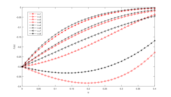
Figure 1: (color online) $\Lambda(u)$ vs. $u$ for the case of $L=2$. The curves calculated from $T-Q$ relation (2.24) and the nested BAEs (2.30)-(2.31) are exactly the same as those obtained from the exact diagonalization of the transfer matrix $t(u)$.

The numerical solutions of BAEs (2.30)-(2.31) and the corresponding eigenvalues of the Hamiltonian (1.1) for $L=2$ is shown in Table 1, while the calculated $\Lambda(u)$ curves for $L=2$ are shown in Figure 1. Those numerical simulations imply that the inhomogeneous $T-Q$ relation (2.24) and the BAEs (2.30)-(2.31) indeed give the correct and complete spectrum of the one-dimensional supersymmetric $t-J$ model with unparallel boundary fields [25, 32, 33].

3 Finite-size effects

In order to study the contribution of the inhomogeneous term (the last term in (2.24)) to the ground state energy, we first consider the $T-Q$ relation without the inhomogeneous term, i.e.,

$$\Lambda_{hom}(u) = w_{3}(u)(\xi+u)(u+\eta)^{2L}\frac{Q(u-\eta)}{Q(u)}-u^{2L}\bar{a}(u)\frac{Q(u-\eta)Q^{(1)}(u+\eta)}{Q(u)Q^{(1)}(u)}$$ (3.1)

$$-u^{2L}\bar{d}(u)\frac{Q^{(1)}(u-\eta)}{Q^{(1)}(u)}.$$

The singular property of the $T-Q$ relation (3.1) gives rise to the associated BAEs

$$\frac{\mu_{j}+(\frac{\eta}{2}-\xi^{\prime})}{\mu_{j}-(\frac{\eta}{2}-\xi^{\prime})}\left(\frac{\mu_{j}+\frac{\eta}{2}}{\mu_{j}-\frac{\eta}{2}}\right)^{2L}=-\prod_{l=1}^{\bar{M}}\frac{\mu_{j}-\lambda_{l}+\frac{\eta}{2}}{\mu_{j}-\lambda_{l}-\frac{\eta}{2}}\frac{\mu_{j}+\lambda_{l}+\frac{\eta}{2}}{\mu_{j}+\lambda_{l}-\frac{\eta}{2}},$$ (3.2)

and

$$\frac{\lambda_{j}-\frac{\eta}{2}}{\lambda_{j}+\frac{\eta}{2}}\frac{(\lambda_{j}+\xi^{\prime})(\lambda_{j}+\xi)}{(\lambda_{j}-\xi^{\prime})(\lambda_{j}-\xi)}$$

$$=-\prod_{k=1}^{M}\frac{(\lambda_{j}-\mu_{k}+\frac{\eta}{2})(\lambda_{j}+\mu_{k}+\frac{\eta}{2})}{(\lambda_{j}-\mu_{k}-\frac{\eta}{2})(\lambda_{j}+\mu_{k}-\frac{\eta}{2})}\prod_{l=1}^{\bar{M}}\frac{(\lambda_{j}-\lambda_{l}-\eta)(\lambda_{j}+\lambda_{l}-\eta)}{(\lambda_{j}-\lambda_{l}+\eta)(\lambda_{j}+\lambda_{l}+\eta)},$$ (3.3)

where we have put $v_{j}=\mu_{j}-\frac{\eta}{2}$.

Assume that $\mu_{j}\rightarrow\mu_{j}i$, $\lambda_{j}\rightarrow\lambda_{j}i$ and $\eta=1$, we obtain

$$\frac{\mu_{j}-(\frac{1}{2}-\xi^{\prime})i}{\mu_{j}+(\frac{1}{2}-\xi^{\prime})i}\left(\frac{\mu_{j}-\frac{i}{2}}{\mu_{j}+\frac{i}{2}}\right)^{2L}=-\prod_{l=1}^{\bar{M}}\frac{\mu_{j}-\lambda_{l}-\frac{i}{2}}{\mu_{j}-\lambda_{l}+\frac{i}{2}}\frac{\mu_{j}+\lambda_{l}-\frac{i}{2}}{\mu_{j}+\lambda_{l}+\frac{i}{2}},$$ (3.4)

and

$$\frac{\lambda_{j}+\frac{i}{2}}{\lambda_{j}-\frac{i}{2}}\frac{(\lambda_{j}-\xi^{\prime}i)(\lambda_{j}-\xi i)}{(\lambda_{j}+\xi^{\prime}i)(\lambda_{j}+\xi i)}$$

$$=-\prod_{k=1}^{M}\frac{(\lambda_{j}-\mu_{k}-\frac{i}{2})(\lambda_{j}+\mu_{k}-\frac{i}{2})}{(\lambda_{j}-\mu_{k}+\frac{i}{2})(\lambda_{j}+\mu_{k}+\frac{i}{2})}\prod_{l=1}^{\bar{M}}\frac{(\lambda_{j}-\lambda_{l}+i)(\lambda_{j}+\lambda_{l}+i)}{(\lambda_{j}-\lambda_{l}-i)(\lambda_{j}+\lambda_{l}-i)}.$$ (3.5)

The corresponding eigenvalue reads

$$E_{hom} = \frac{\eta}{2}\frac{d\ln\Lambda_{hom}(u)}{du}\Big{|}_{u=0}-\frac{\eta}{2\xi}+\frac{\eta-2\xi^{\prime}}{2(\eta-\xi^{\prime})}+2M-L+1$$ (3.6)

$$= -\sum_{k=1}^{M}\frac{1}{\mu_{k}^{2}+\frac{1}{4}}+2M.$$

Now, we consider the contribution of the inhomogeneous term in Eq. (2.24) to the ground state energy of the system. In order to this, we should analyze the distribution of Bethe roots in the BAEs (3.4) and (3.5). For $\xi<0$ and $\xi^{\prime}<1$ (equivalent to $\chi_{1}>1$ and $\chi_{L}<1$), by using the standard thermodynamic Bethe ansatz method and taking the limit of temperature tending to zero, we find that all the Bethe roots are real at the ground state in the region of $\xi<0$ and $\xi^{\prime}\leq 1/2$ (equivalent to $\chi_{1}>1$ and $0\leq\chi_{L}<1$). While in region of $\xi<0$ and $1/2<\xi^{\prime}<1$ (equivalent to $\chi_{1}>1$ and $\chi_{L}<0$), besides the real Bethe roots, there exists an imaginary Bethe root which corresponds to a boundary bound state. Let us discuss them separately.

3.1 Region of $\xi<0$ and $\xi^{\prime}\leq 1/2$

Firstly, we consider the case of $\xi<0$ and $\xi^{\prime}\leq 1/2$ [21, 25], in which all the Bethe roots are real at the ground state. Taking the logarithm of BAEs (3.4)-(3.5), we obtain

$$2\pi I_{j} = 2\arctan\left(\frac{2\mu_{j}}{1-2\xi^{\prime}}\right)+4L\arctan(2\mu_{j})$$ (3.7)

$$-\sum_{l=1}^{\bar{M}}2\arctan(2(\mu_{j}-\lambda_{l}))+2\arctan(2(\mu_{j}+\lambda_{l})),$$

$$2\pi J_{j} = 2\arctan(2\lambda_{j})-2\arctan\left(\frac{\lambda_{j}}{\xi^{\prime}}\right)-2\arctan\left(\frac{\lambda_{j}}{\xi}\right)$$ (3.8)

$$+\sum_{k=1}^{M}2\arctan(2(\lambda_{j}-\mu_{k}))+2\arctan(2(\lambda_{j}+\mu_{k}))$$

$$-\sum_{l=1}^{\bar{M}}2\arctan(\lambda_{j}-\lambda_{l})+2\arctan(\lambda_{j}+\lambda_{l}),$$

where $I_{j}$ and $J_{j}$ are both quantum numbers which determine the eigenenergy and the corresponding eigenstates. It is well-known that the size of the system $L$, with either even or odd value, gives the same physics properties in the thermodynamic limit. Therefore, for simplicity, we set $L$ as an even number.

We define the contribution of the inhomogeneous term to the ground state energy as

$$E_{inh}=E_{hom}-E_{true}.$$ (3.9)

Here $E_{hom}$ is the energy of the supersymmetric $t-J$ model calculated by the eigenvalue (3.6) and the BAEs (3.7)-(3.8). $E_{true}$ is the energy of the Hamiltonian (1.1), which can be obtained by using the density matrix renormalization group (DMRG) [34]. For the ground state, the number of Bethe roots reduces to $M=L/2$ and $\bar{M}=0$,

$$2\pi I_{j}=2\arctan\left(\frac{\mu_{j}}{\zeta}\right)+4L\arctan(2\mu_{j}),~{}j=1,\cdots,M,$$ (3.10)

where $I_{j}\in\{1,2,\cdots,L/2\}$, $\zeta=1/2-\xi^{\prime}$ and $\zeta\geq 0$. Then “ground state energy” $E_{hom}$ is given by equation (3.6) with the constraint (3.10).

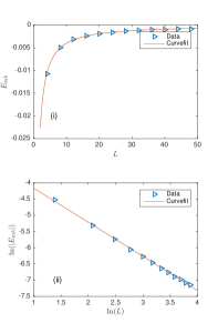
(a) $\theta=\pi/5$

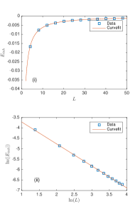
(b) $\theta=\pi/4$

(c) $\theta=\pi/2$

Figure 2: The contribution of the inhomogeneous term to the ground state energy $E_{inh}$ versus the system size $L$. The data can be fitted as $E_{inh}=\gamma L^{\beta}$ [or $\ln(|E_{inh}|)=p\ln(L)+q$]. Here $\xi=-0.1$, $\zeta=0.05$, $\theta^{\prime}=0$, $\phi=\phi^{\prime}=0$, (a) $\theta=\pi/5$, $\gamma=-0.0478$ and $\beta=-1.080$; (b) $\theta=\pi/4$, $\gamma=-0.0755$ and $\beta=-1.087$; (c) $\theta=\pi/2$, $\gamma=-0.2871$ and $\beta=-1.073$. Due to the fact $\beta<0$ [or $p<0$], when the $L$ tends to infinity, the contribution of the inhomogeneous term tends to zero.

The values of $E_{inh}$, the contribution of the inhomogeneous term to the ground state energy, versus the system size $L$ are shown in Figure 2. From the fitting, we find the power law relation between $E_{inh}$ and $L$, i.e., $E_{inh}=\gamma L^{\beta}$. Due to the fact that $\beta\approx-1$, the value of $E_{inh}$ tends to zero when the size of the system tends to infinity, which means that the inhomogeneous term in the $T-Q$ relation (2.24) can be neglected in the thermodynamic limit $L,N,M\rightarrow\infty$ with $N/L$ and $M/L$ kept fixed. Therefore, the two boundaries are decoupled from each other completely in the thermodynamic limit. When $h=0$, the unparallel boundary fields degenerates into the parallel one. At this point, the contribution of the inhomogeneous term to the ground state energy $E_{inh}$ is equal to 0.

3.2 Region of $\xi<0$ and $1/2<\xi^{\prime}<1$

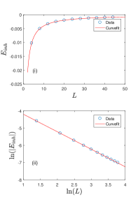
(a) $\theta^{\prime}=0.80$

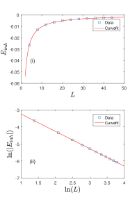
(b) $\theta^{\prime}=1.20$

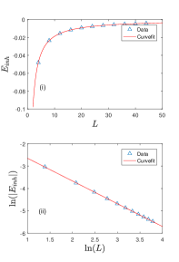
(c) $\theta^{\prime}=1.57$

Figure 3: The values of $E_{inh}$ versus the system size $L$. The data can be fitted as $E_{inh}=\tilde{\gamma}L^{\tilde{\beta}}$ [or $\ln(|E_{inh}|)=\tilde{p}\ln(L)+\tilde{q}$]. Here $\xi=-0.1$, $\xi^{\prime}=0.95$, $\theta=0.15$, $\phi=\phi^{\prime}=0$, (a) $\theta^{\prime}=0.80$, $\tilde{\gamma}=0.0423$ and $\tilde{\beta}=-1.0250$; (b) $\theta^{\prime}=1.20$, $\tilde{\gamma}=0.1097$ and $\tilde{\beta}=-1.0260$; (c) $\theta^{\prime}=1.57$, $\tilde{\gamma}=0.1988$ and $\tilde{\beta}=-1.0250$. Due to the fact $\tilde{\beta}<0$ [or $\tilde{p}<0$], when the $L$ tends to infinity, the $E_{inh}$ tends to zero.

In the region of $\xi<0$ and $1/2<\xi^{\prime}<1$, one of the Bethe roots at the ground state goes to $(\frac{1}{2}-\xi^{\prime})i$ when the system-size $L$ tends to infinity [25, 35, 36, 37]. We note the value of this Bethe root is related with the boundary parameter $\xi^{\prime}$. Without losing generality, we assume that $\mu_{M}=(\frac{1}{2}-\xi^{\prime})i+\mathcal{O}(e^{-\delta L})=\zeta i+\mathcal{O}(e^{-\delta L})$ where $M=L/2$ and $\delta$ is a small positive number to account for the finite size deviations. This Bethe root contributes a negative bare energy if $-1/2<\zeta<0$. The remaining Bethe roots should take real values and satisfy the following BAEs

$$\frac{\mu_{j}-\zeta i}{\mu_{j}+\zeta i}\left(\frac{\mu_{j}-\frac{i}{2}}{\mu_{j}+\frac{i}{2}}\right)^{2L}=-1,~{}~{}~{}j=1,2,\cdots,M-1.$$ (3.11)

Taking the logarithm of Eq.(3.11), we have

$$2\pi I_{j}=2\arctan\left(\frac{\mu_{j}}{\zeta}\right)+4L\arctan(2\mu_{j}),~{}j=1,\cdots,M-1,$$ (3.12)

where the quantum numbers $\{I_{j}\}$ are chosen as $\{1,2,\cdots,L/2-1\}$. The corresponding energy reads

$$E_{hom}=-\sum_{k=1}^{M-1}\frac{1}{\mu_{k}^{2}+\frac{1}{4}}-\frac{1}{\frac{1}{4}-\zeta^{2}}+2M.$$ (3.13)

The values of $E_{inh}$ versus the system size $L$ are shown in Figure 3. From the fitted curves in Figure 3, we see that the $E_{inh}$ also satisfies the scaling law $L^{-1}$. Therefore, the contribution of the inhomogeneous term to the ground state energy in the thermodynamic limit is zero and we have $E_{hom}=E_{ture}\equiv E$. In addition, the results indicating that the boundary bound state should be stable. The surface energy will compute in the next section.

4 Surface energy

In order to analyze the influence of the boundary fields, now we calculate the surface energy [38, 39, 40] of the system.

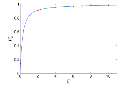
Figure 4: The surface energies versus the boundary parameters. The blue curves are the ones calculated from equation (4.7), while the red points ($\xi=-0.1$, $\theta=\pi/5$, $\phi=0$, $\theta^{\prime}=0$ and $\phi^{\prime}=0$) and green stars ($\xi=-5$, $\theta=\pi/4$, $\phi=0$, $\theta^{\prime}=2\pi/3$ and $\phi^{\prime}=0$) are the ones obtained from the Hamiltonian (1.1) with the BST algorithms.

4.1 Region of $\xi<0$ and $\xi^{\prime}\leq 1/2$

Define $Z(\mu_{j})=\frac{I_{j}}{2L}$, then the BAEs (3.10) can be rewritten as

$$Z(\mu_{j})=\frac{1}{2\pi}\left[\frac{1}{2L}\Xi_{2\zeta}(\mu_{j})+\Xi_{1}(\mu_{j})\right],$$ (4.1)

where $\Xi_{n}(x)=2\arctan(2x/n)$. It turns to be a continuous function in the thermodynamic limit as the distribution of Bethe roots is continuous, i.e., $Z(\mu_{j})\to Z(u)$. In the thermodynamic limit, the density distributions are determined by

$$\rho(u)+\rho^{h}(u)=\frac{dZ(u)}{du}.$$ (4.2)

Taking the derivative of $Z(u)$ with respect to $u$, we obtain the density of states as

$$\rho(u)=a_{1}(u)+\frac{1}{2L}\left[a_{2\zeta}(u)-\delta(u)\right],$$ (4.3)

where

$$a_{n}(u)=\frac{1}{2\pi}\frac{n}{u^{2}+\frac{n^{2}}{4}}.$$ (4.4)

The ground state energy is equal to

$$E=-2\pi L\int_{-B}^{B}\left(a_{1}(\mu)\right)^{2}d\mu+2M-\pi\int_{-B}^{B}a_{1}(\mu)\left[a_{2\zeta}(\mu)-\delta(\mu)\right]d\mu,$$ (4.5)

and the energy density of the ground state is

$$e_{g}=-2\pi\int_{-B}^{B}\left(a_{1}(\mu)\right)^{2}d\mu+1+{O}(L^{-1}),$$ (4.6)

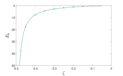
Figure 5: The surface energies versus the boundary parameters. The blue curves are the ones calculated from equation (4.10), while the red points ($\xi=-0.1$, $\theta=0.3\pi$, $\phi=0$, $\theta^{\prime}=0.7\pi$ and $\phi^{\prime}=0$) and green stars ($\xi=-0.1$, $\theta=0.17\pi$, $\phi=0$, $\theta^{\prime}=0.62\pi$ and $\phi^{\prime}=0$) are the ones obtained from the Hamiltonian (1.1) with the BST algorithms.

where $B=\frac{1}{2}+\frac{\pi-2\arctan\left(\frac{1}{2\zeta}\right)}{4L+\frac{4\zeta}{1+4\zeta^{2}}}$. The energy density $e_{g}$ is equal to $-2/\pi$ in the thermodynamic limit, which is the same with that of the periodic case [41]. The surface energy then can be given by

$$E_{b}(\zeta)=\lim_{L\rightarrow\infty}\left[E_{0}(L;\zeta)-E_{0}^{periodic}(L)\right]$$

$$\quad\quad\quad=-\pi\int_{-\frac{1}{2}}^{\frac{1}{2}}a_{1}(\mu)a_{2\zeta}(\mu)d\mu+\frac{2}{\pi}\arctan\left(\frac{1}{2\zeta}\right)+1.$$ (4.7)

By using the relation (4.7), one can calculate the surface energy of the one-dimensional supersymmetric $t-J$ model with unparallel boundary fields. The results are shown in Figure 4, where the blue solid lines are the surface energy calculated by using the relation (4.7) and the red points and green stars are data obtained by employing the BST algorithms [42] to solve the surface energy of the Hamiltonian (1.1) in the thermodynamic limit. Specifically, for one of the red points or green stars, we first calculate the ground state energy $E_{0}(L)$ with $L=4,8,\cdots,48$ by the DMRG. Then, the large-$L$ extrapolation of the surface energy was performed using BST algorithms from the sequence $E_{0}(4)-4e_{g}^{\infty}$, $E_{0}(8)-8e_{g}^{\infty}$, $\cdots$, $E_{0}(48)-48e_{g}^{\infty}$. Note that $e_{g}^{\infty}=-2/\pi$. From the Figure 4, we can see that the analytical and numerical results agree with each other very well for all tunable parameters. The surface energy increased with the increase of $\zeta$. Taking the $\zeta\rightarrow 0$ limit of Eq.(4.7), we have $E_{b}(\zeta\rightarrow 0)=0$. Taking the $\zeta\rightarrow\infty$ limit of Eq.(4.7), we have $E_{b}(\zeta\rightarrow\infty)=1$.

4.2 Region of $\xi<0$ and $1/2<\xi^{\prime}<1$

In this region, the ground state energy of the system in the thermodynamic limit reads

$$E=-2\pi L\int_{-\tilde{B}}^{\tilde{B}}\left(a_{1}(\mu)\right)^{2}d\mu+2M-\pi\int_{-\tilde{B}}^{\tilde{B}}a_{1}(\mu)[a_{2\zeta}(\mu)-\delta(\mu)]d\mu-\frac{1}{\frac{1}{4}-\zeta^{2}},$$ (4.8)

and the energy density of the ground state is

$$e_{g}=-2\pi\int_{-\tilde{B}}^{\tilde{B}}\left(a_{1}(\mu)\right)^{2}d\mu+1+{O}(L^{-1}),$$ (4.9)

where $\tilde{B}=\frac{1}{2}-\frac{\pi+2\arctan\left(\frac{1}{2\zeta}\right)}{4L+\frac{4\zeta}{1+4\zeta^{2}}}$. The surface energy is given by

$$E_{b}(\zeta)=-\pi\int_{-\frac{1}{2}}^{\frac{1}{2}}a_{1}(\mu)a_{2\zeta}(\mu)d\mu+\frac{2}{\pi}\arctan\left(\frac{1}{2\zeta}\right)+3-\frac{1}{\frac{1}{4}-\zeta^{2}}.$$ (4.10)

The results are shown in Figure 5. Again, we see that the analytical results and the numerical ones agree with each other very well.

The surface energy can be written in unified forms as

$$E_{b}(\zeta)=-\pi\int_{-\frac{1}{2}}^{\frac{1}{2}}a_{1}(\mu)a_{2\zeta}(\mu)d\mu+\frac{2}{\pi}\arctan\left(\frac{1}{2\zeta}\right)+\Delta,$$ (4.11)

where $\Delta=1$ when $\xi<0$ and $\xi^{\prime}\leq 1/2$, and $\Delta=3-\frac{1}{\frac{1}{4}-\zeta^{2}}$ when $\xi<0$ and $1/2<\xi^{\prime}<1$.

5 Conclusions

In this paper, we have studied the thermodynamic limit of the one-dimensional supersymmetric $t-J$ with unparallel boundary fields. It is shown that the contribution of the inhomogeneous term to the ground state energy is inversely proportional with $L$, i.e., $E_{inh}\propto L^{-1}$. This fact enables us to calculate the surface energy (4.7) and (4.10), which is same as that for the case of parallel boundary fields [21]. Moreover, it implies that the inhomogeneous term in (2.24) surely gives some contributions to the other physical qualities such as the boundary conformal charge, which are related to the coefficients in the expansion of energy $E$ in terms of the powers of $L^{-1}$ (namely, the coefficient of $L^{-1}$ corresponds to the conformal charge [36]).

The method used in this paper can be generalized to study the thermodynamic limit and surface energy of other models related to rational $R$-matrices, such as the spin-$s$ XXX chain or the $su(n)$ spin chain with unparallel boundary fields. These results may be applied to the theory of ultra-cold atom systems, asymmetric simple exclusion process.

References

- [1] J. Spalek and A. M. Oles, Physica B+C 86 (1977) 375.
- [2] K. A. Chao, J. Spalek and A. M. Oles, J. Phys. C: Solid State Phys. 10 (1977) L271.
- [3] F. C. Zhang and T. M. Rice, Phys. Rev. B 37 (1988) 3759.
- [4] P. W. Anderson, Science 235 (1987) 1196.
- [5] F. H. L. Essler, V. E. Korepin and K. Schoutens, Phys. Rev. Lett. 68 (1992) 2960.
- [6] Y. Q. Chong, V. Murg, V. E. Korepin and F. Verstraete, Phys. Rev. B 91 (2015) 195132.
- [7] S. Reja, J. V. D. Brink and S. Nishimoto, Phys. Rev. Lett. 116 (2016) 067002.
- [8] F. H. L. Essler and V. E. Korepin, Phys. Rev. B 46 (1992) 9147.
- [9] H. Fan, M. Wadati and X.-M. Wang, Phys. Rev. B 61 (2000) 3450.
- [10] W. Galleas, Nucl. Phys. B 777 (2007) 352.
- [11] E. K. Sklyanin, J. Phys. A: Math. Gen. 21 (1988) 2375.
- [12] P. B. Wiegmann, Phys. Rev. Lett. 60 (1988) 821.
- [13] D. Forster, Phys. Rev. Lett. 63 (1989) 2140.
-
[14]
A. Foerster and M. Karowski, Phys. Rev. B 46 (1992) 9234;
A. Foerster and M. Karowski, Nucl. Phys. B 396 (1993) 611. - [15] B. Sutherland, Phys. Rev. B 12 (1975) 3795.
- [16] P. Schlottmann, Phys. Rev. B 36 (1987) 5177.
- [17] H. J. Schulz, Phys. Rev. Lett. 64 (1990) 2831.
- [18] H. M. Babujian and R. Flume, Mod. Phys. Lett. A 9 (1994) 2029.
-
[19]
H. M. Babujian, A. Foerster and M. Karowski, J. Phys. A: Math. Theor. 41 (2008) 275202;
H. M. Babujian, A. Foerster and M. Karowski, J. Phys. A: Math. Theor. 45 (2012) 055207. - [20] A. S. Mishchenko and N. Nagaosa, Phys. Rev. Lett. 93 (2004) 036402.
- [21] F. H. L. Essler, J. Phys. A: Math. Gen. 29 (1996) 6183.
- [22] J. Sirker and A. Klumper, Phys. Rev. B 66 (2002) 245102.
- [23] M. Takahashi, Thermodynamics of One-Dimensional Solvable Models, Cambridge University Press, 1999.
- [24] X. Zhang, J. Cao, W.-L. Yang, K. Shi and Y. Wang, J. Stat. Mech. (2014) P04031.
- [25] Y. Wang, W.-L. Yang, J. Cao and K. Shi, Off-Diagonal Bethe Ansatz for Exactly Solvable Models, Springer Press, 2015.
- [26] P. Sun, F. Wen, K. Hao, J. Cao, G.-L. Li, W.-L. Yang and K. Shi, J. High Energy Phys. 07 (2017) 051.
- [27] J. Cao, W.-L. Yang, K. Shi and Y. Wang, Phys. Rev. Lett. 111 (2013) 137201.
- [28] R. I. Nepomechie and C. Wang, J. Phys. A 47 (2014) 032001.
- [29] Y.-Y. Li, J. Cao, W.-L. Yang, K. Shi and Y. Wang, Nucl. Phys. B 884 (2014) 17.
- [30] F. Wen, T. Yang, Z.-Y. Yang, J. Cao, K. Hao and W.-L. Yang, Nucl. Phys. B 915 (2017) 119.
- [31] L. Corwin, Y. Neeman and S. Sternberg, Rev. Mod. Phys. 47 (1975) 573.
- [32] R. I. Nepomechie, J. Phys. A 46 (2013) 442002.
- [33] N. Kitanine, J.-M. Maillet and G. Niccoli, J. Stat. Mech. (2014) P05015.
- [34] B. Bauer, L. D. Carr, H. G. Evertz, A. Feiguin, J. Freire, S. Fuchs, L. Gamper, J. Gukelberger, E. Gull, S. Guertler, A. Hehn, R. Igarashi, S. V. Isakov, D. Koop, P. N. Ma, P. Mates, H. Matsuo, O. Parcollet, G. Pawöwski, J. D. Picon, L. Pollet, E. Santos, V. W. Scarola, U. Schollwöck, C. Silva, B. Surer, S. Todo, S. Trebst, M. Troyer, M. L. Wall, P. Werner and S. Wessel, J. Stat. Mech. (2011) P05001.
- [35] S. Skorik and H. Saleur, J. Phys. A: Math. Gen. 28 (1995) 6605.
- [36] Y. Wang, J. Voit and Fu-Cho Pu, Phys. Rev. B 54 (1996) 8491.
- [37] Y. Wang, Phys. Rev. B 56 (1997) 14045.
- [38] M. Gaudin, Phys. Rev. A 4 (1971) 386.
- [39] C. Hamer, G. Quispel and M. T. Batchelor, J. Phys. A 20 (1987) 5677.
- [40] M. T. Batchelor and C. Hamer, J. Phys. A 23 (1990) 761.
- [41] C. K. Lai, J. Math. Phys. 15 (1974) 1675.
- [42] M. Henkel and G. Schutz, J. Phys. A 21 (1988) 2617.