Self-gravitating $\boldsymbol{\Lambda}$-media

Abstract

We address the question whether a medium featuring $p+\rho=0$, dubbed $\Lambda$-medium, has to be necessarily a cosmological constant. By using effective field theory, we show that this is not the case for a class of media comprising perfect fluids, solids and special super solids, providing an explicit construction. The low energy excitations are non trivial and lensing, the growth of large scale structures can be used to clearly distinguish $\Lambda$-media from a cosmological constant.

1 Introduction

We do not know yet the nature of dark energy, though we have some information on its equation of state. Actually, assuming a constant equation of state, observations indicate $p+\rho\approx 0$, which points toward the simplest possibility: a cosmological constant (CC). Suppose that the upcoming large scale structure surveys will establish that $w\equiv p/\rho\equiv-1$, can we conclude then that dark energy behaves as a CC? For a pure CC we have $\rho=-p=$constant and the corresponding fluctuations are zero: $\delta\rho=\delta p=0$; moreover gravitational waves propagate with a massless dispersion relation $\omega^{2}=k^{2}$. The goal of this paper is to show that is possible to construct simple field theory models based on an action principle, describing what we call a $\Lambda$-medium featuring $p+\rho=0$ as a non-perturbative equation of state. Though in a Friedman-Lemaitre-Robertson-Walker (FLRW) background a $\Lambda$-medium is completely equivalent to a CC this is not the case when perturbations are introduced. Indeed, we still have $\delta p=-\delta\rho$, but with non-trivial perturbations.
The starting point is the assumption that dark energy can be effectively described as an isotropic medium whose low-energy excitations are phonon-like. Such behaviour is rather common in condensed matter systems but also in cosmology.

The outline of the paper is the following. In section 2 we briefly recall the basics of self gravitating media that represent the general framework of which $\Lambda$-media are a very special subset. $\Lambda$-media are introduced in section 3 together with their thermodynamical properties. Section 4 is devoted to the study of the conditions under which $\Lambda$-media are stable under linear perturbations around flat space. Scalar cosmological perturbation are studied in section 5 while the tensor ones are analysed in section 5.1. The study of how the growth of structure is modified in the presence of $\Lambda$-media is given in 6. Finally, section 7 contains our conclusions.

2 Self-Gravitating Media

The key tool we use is the effective field theory (EFT) description of the dynamics of media [1, 2, 3, 4, 5, 6, 7, 8, 9] according to which the low energy excitations (phonons) can be described by a classical theory of four derivatively coupled scalar fields $\varphi^{A}$, $A=0,1,2,3$. Among the various action principle formulations of the dynamics of media [10, 11, 12, 13, 14, 15], the EFT framework is formulated in terms of unconstrained fields and it is capable to describe perfect fluids, super fluids, solids and super solids depending on the internal symmetries of the action which translates in the form of the energy momentum tensor (EMT). A similar formalism was used in the contest of inflation [16, 17, 18, 19, 20], though barring any special relation among operators realising $p+\rho=0$. Following the notations of [8, 9], the leading operators in the EFT for homogeneous media, invariant under the shift symmetry $\varphi^{A}\rightarrow\varphi^{A}+\lambda^{A}$ for constant $\lambda^{A}$, can be written in terms of the matrix

$$C^{AB}=g^{\mu\nu}\partial_{\mu}\varphi^{A}\partial_{\nu}\varphi^{B}\,,$$ (2.1)

and the velocity fields $u_{\mu}$ and $\mathcal{V}_{\mu}$

$$u^{\mu}=-\frac{\epsilon^{\mu\nu\alpha\beta}}{6\,b\sqrt{-g}}\epsilon_{abc}\,\partial_{\nu}\varphi^{a}\,\,\partial_{\alpha}\varphi^{b}\,\partial_{\beta}\varphi^{c}\,\qquad\mathcal{V}_{\mu}=-\frac{\partial_{\mu}\varphi^{0}}{\sqrt{-X}}\,,$$ (2.2)

where $g_{\mu\nu}$ is the space-time metric, $b=\sqrt{\det\left(B^{ij}\right)}$, with $B^{ij}\equiv C^{ij}$ and $X=C^{00}$. Small latin indices like $i,j$, assume the values 1,2,3 while greek and capital latin ones the values 0,1,2,3; we shall also denote by $\boldsymbol{B}$ the $3\times 3$ matrix with matrix elements $B^{ij}$. Being $u^{\mu}\partial_{\mu}\varphi^{j}=0$, $\varphi^{j}$ can be interpreted as the spatial Lagrangian (comoving) coordinates of the medium, while $\varphi^{0}$ represents the clock’s medium. The action of a self-gravitating medium in the presence of gravity is

$$S=M_{\text{Pl}}^{2}\;\int d^{4}x\;\sqrt{-g}\,R+\int d^{4}x\sqrt{-g}\;U\left(C^{AB}\right)\,;$$ (2.3)

where $R$ is the Ricci scalar, $M_{\text{Pl}}=(16\pi G)^{-1/2}$ is the Planck mass and $U$ is the medium Lagrangian depending on the derivative of the Stückelberg fields $\varphi^{A}$. At leading order we have a total of 9 operators $Y,\;X,\;\tau_{1,2,3},\;y_{0,1,2,3}$ (compatible with isotropy, implemented as a global internal spatial $SO(3)$ symmetry $\varphi^{i}\rightarrow R^{i}_{\phantom{i}j}\varphi^{j}$, with the constant matrix $\mathbf{R}\in SO(3)$) defined as

$$Y=u^{\mu}\partial_{\mu}\varphi^{0},\qquad\tau_{n}=\text{Tr}\left(\boldsymbol{B}^{n}\right),\qquad y_{n}=\text{Tr}\left(\boldsymbol{B}^{n}\,\boldsymbol{Z}\right)$$ (2.4)

where $\boldsymbol{Z}$ is $3\times 3$ matrix with matrix elements $Z^{ij}=C^{0i}C^{0j}$ (note that $b=(\tau_{1}^{3}-3\;\tau_{2}\;\tau_{1}+2\;\tau_{3})/6$). Moreover, we define the operators $w_{n}=\text{Tr}(\boldsymbol{W}^{n})$, where $\boldsymbol{W}\equiv\boldsymbol{B}-\boldsymbol{Z}/X$.
Interestingly, the EFT formalism allows also to give a thermodynamical interpretation [21, 9] by which some combinations of operators are related to thermodynamical variables.

3 $\Lambda$-Media

From the action (2.3), the energy momentum tensor (EMT) for the most generic media has the following structure

$$T_{\mu\nu}=-\frac{2}{\sqrt{-g}}\frac{\delta S}{\delta g^{\mu\nu}}=p\,h_{\mu\nu}+\rho\,u_{\mu}u_{\nu}+2\,q_{(\mu}u_{\nu)}+\pi_{\mu\nu}$$ (3.1)

where $\rho=u^{\mu}u^{\nu}T_{\mu\nu}$, $p=h^{\mu\nu}T_{\mu\nu}/3$, $q_{\mu}$ satisfies $u_{\mu}q^{\mu}=0$ and $\pi^{\mu}_{\phantom{\mu}\mu}=u^{\mu}\pi_{\mu\nu}=0$.
Depending on the internal symmetries, we can select some special combinations of the operators appearing in the Lagrangian, corresponding to particular classes of media. For instance, fluids and super fluids $U(X,Y,b)$ are protected by invariance under volume preserving diffeomorphisms

$$\varphi^{a}\rightarrow\psi^{a}(\varphi^{b})\,,\qquad\text{det}\left|\partial\psi^{a}/\partial\varphi^{b}\right|=1\,.$$ (3.2)

Since for $\Lambda$-media $w=-1$, the condition $p(U)=-\rho(U)$ at the non-perturbative level is equivalent to a differential equation for $U$, which can be solved in terms of the basic operators considered as independent variables.
Let us describe this procedure for the following classes of media

• solids, characterised by $U(Y,\tau_{n})$

• special super solids, characterised by $U(X,w_{n})$

• perfect fluids, characterised by $U(Y,b)$.

Solids are selected by the invariance under the internal symmetry [22, 8]

$$\varphi^{0}\to\varphi^{0}+f(\varphi^{j})$$ (3.3)

and the thermodynamical dictionary is given in Table 1. The entropy per particle $\sigma=s/n$ is constant in time

$$\dot{\sigma}=u^{\mu}\partial_{\mu}\sigma=0\,.$$ (3.4)

From the non-perturbative expression for $p$ and $\rho$ in Table 1, imposing $w=-1$ gives

$$Y\;U_{Y}-\frac{2}{3}\sum_{m=1}^{3}m\;\tau_{m}U_{\tau_{m}}=0\,,$$ (3.5)

which reduces the original dependence of $U$ from the original four operators down to the following three special combinations

$$U^{\Lambda}_{S}=U\left(Y\tau_{1}^{3/2},\frac{\tau_{2}}{\tau_{1}^{2}},\frac{\tau_{3}}{\tau_{1}^{3}}\right)$$ (3.6)

invariant under the Lifshitz scaling [23, 16, 24]

$$\left\{\begin{array}[]{lr}\varphi^{0}\rightarrow&\lambda^{-3}\,\varphi^{0}\\ \varphi^{j}\rightarrow&\lambda\,\varphi^{j}\end{array}\right.\,.$$ (3.7)

An interesting subcase is the isentropic solid with an entropy per particle constant in spacetime, described by $U(\tau_{n})$ (where only the spatial Stückelberg $\varphi^{j}$ are present) and characterised by $s=0$. In particular, $\Lambda$-isentropic solids are described by

$$U^{\Lambda}_{IS}=U\left(\frac{\tau_{2}}{\tau_{1}^{2}},\frac{\tau_{3}}{\tau_{1}^{3}}\right)\,.$$ (3.8)

Special super solids $U(X,w_{n})$ are selected by the invariance under the internal symmetry [22, 25, 8, 9]

$$\varphi^{j}\rightarrow\varphi^{j}+f^{j}(\varphi^{0})\,.$$ (3.9)

$\Lambda$-special super solids are obtained imposing $p=-\rho$ for the expressions in Table 1; we have

$$U^{\Lambda}_{SS}=U\left(Xw_{1}^{3},\frac{w_{2}}{w_{1}^{2}},\frac{w_{3}}{w_{1}^{3}}\right)\,,$$ (3.10)

which is again invariant under the Lifshitz scaling (3.7). Similar media were studied in a cosmological setting in [23, 26] and also in the contest of spherically symmetric solutions in massive gravity [27, 28].
Isentropic special super solids, described by $U(w_{n})$, are invariant under (3.9) and [8]

$$\varphi^{0}\rightarrow\varphi^{0}+f(\varphi^{0})\,.$$ (3.11)

Remarkably, a proposal for a UV completion for isentropic special super solids involving at LO the scalar operators $w_{1}$ and $w_{2}$ was put forward in [29], where the temporal Stückelberg $\varphi^{0}$ is embedded into the khronometric model and the spatial Stückelberg $\varphi^{j}$ are coupled to a triplet of Higgs vector fields.
The symmetry (3.11) forbids the operator $X$ in $U^{\Lambda}_{SS}$ and we conclude that $\Lambda$-isentropic special super solids are described by

$$U^{\Lambda}_{ISS}=U\left(\frac{w_{2}}{w_{1}^{2}},\frac{w_{3}}{w_{1}^{3}}\right)\,.$$ (3.12)

Finally, perfect fluids are protected by the symmetries (3.2) and (3.3); their Lagrangian is of the form $U(Y,b)$.
$\Lambda$-perfect fluids with $p+\rho=0$ have the following Lagrangian [8]

$$U^{\Lambda}_{PF}=U(Yb)$$ (3.13)

which is protected by the enhanced symmetry

$$\varphi^{A}\rightarrow\psi^{A}(\varphi^{B})\,,\qquad\text{det}\left|\partial\psi^{A}/\partial\varphi^{B}\right|=1\,.$$ (3.14)

The $\Lambda$-perfect fluid EMT simply reads $T_{\mu\nu}=p\,g_{\mu\nu}$ whose conservation leads directly to $\rho=$constant. Although a $\Lambda$-perfect fluid is similar to a CC, the non-vanishing entropy per particle indicates that underlying degrees of freedom are present. Moreover, the Stückelberg fields satisfy non-trivial equations of motion in order to keep the combination $b\,Y$ constant.
Differently from fluids, anisotropic stress in solids allows to have a conserved energy-momentum tensor, $p+\rho=0$ and non-trivial gradient for the pressure and the energy density. Actually, for a solid $T_{\mu\nu}=p\;g_{\mu\nu}+\pi_{\mu\nu}\;$where $\pi_{\mu\nu}$ is the anisotropic stress; from the conservation of the energy-momentum tensor we get

$$p=-\rho,\qquad\dot{p}=\pi_{\mu\nu}\;\nabla^{\nu}\,u^{\mu}=\pi_{\mu\nu}\;\sigma^{\mu\nu},\qquad{\cal D}_{\mu}p=-{\cal D}^{\nu}\pi_{\mu\nu}-a^{\nu}\pi_{\mu\nu}$$ (3.15)

where $u^{\alpha}\nabla_{\alpha}p\equiv\dot{p}$ and we have used the standard decomposition of the covariant derivative of the velocity in terms of rotation and shear according with $\nabla_{\nu}\,u_{\mu}=\sigma_{\nu\mu}+\omega_{\nu\mu}+\nabla_{\alpha}u^{\alpha}/3\;h_{\nu\mu}-u_{\nu}\;a_{\mu}$ and ${\cal D}^{\mu}=h^{\mu}_{\nu}\,\nabla^{\nu}$, $a^{\mu}=u^{\nu}\nabla_{\nu}u^{\mu}$. Remarkably, the relations (3.15) are intrinsically different from the corresponding relations for a CC

$$p=-\rho=-\Lambda,\qquad\nabla_{\mu}\,p=0\;\;\Rightarrow\;\;p=-\Lambda\,.$$ (3.16)

For a FRW background (3.15) and (3.16) coincide, while for a perturbed FRW metric deviations from a CC are present already at the first order.

	$U(Y,\tau_{n})$	$U(X,w_{n})$	$U(Y,b)$
$\rho$	$-U+Y\;U_{Y}$	$-U+2XU_{X}$	$-U+Y\;U_{Y}$
$p$	$U-\frac{2}{3}\sum_{m}m\;\tau_{m}U_{\tau_{m}}$	$U-\frac{2}{3}\sum_{m}m\;w_{m}U_{w_{m}}$	$U-b\;U_{b}$
$n$	$\tau_{m}^{3/(2m)}$	$w_{m}^{3/(2m)}$	$b$
$s$	$U_{Y}$	$-2\sqrt{-X}U_{X}$	$U_{Y}$

Table 1: Thermodynamical correspondence

4 Dynamical Stability

Since $\Lambda$-media are very particular, it is important to study their stability. Though self-gravitating media can have a familiar Jeans-like instability at some scale $k_{J}$, no instabilities should be present at very large $k$. In this regime, curvature and the mixing of the Stückelberg fields with gravity are negligible and, much like in spontaneously broken gauge theories, the ultraviolet behaviour is captured by the Stückelberg fluctuations. One can forget about gravity and simply study the effective quadratic Lagrangian obtained expanding $U$ around Minkowski space

$$\varphi^{0}=t+\pi_{0}(t,\vec{x}),\ \ \varphi^{j}=x^{j}+V^{j}(t,\vec{x})+\partial^{j}\pi_{L}(t,\vec{x})$$ (4.1)

with $\partial_{j}V^{j}=0$. As discussed in [9], the dynamics of linear perturbations is controlled by five parameters $\{M_{b}\}$ (with $b=0,1,..,4$), expressed in terms of first and second partial derivatives of the Lagrangian $U$ with respect to the basic operators , their expressions are given in the appendix. These parameters are related to the mass terms of the metric fluctuations $h_{00}$, $h_{0i}$ and $h_{ij}$ in the unitary gauge appearing in rotational invariant massive gravity, see [31, 25, 32] and [33] for the non-perturbative structure.
The propagation of scalar perturbations is controlled by two mass parameters: if $\hat{M}_{0}\neq 0$ and $\hat{M}_{1}+\bar{p}+\bar{\rho}\neq 0$ the total energy in the scalar sector is given by

$$\begin{split}E_{s}=\hat{M}_{0}\;\pi_{0}^{\prime}{}^{2}+\frac{k^{2}}{2}\,\left(\hat{M}_{1}+\bar{p}+\bar{\rho}\right)\;\pi_{L}^{\prime}{}^{2}+k^{4}\,\left(\hat{M}_{2}-\hat{M}_{3}\right)\;\pi_{L}^{2}-\frac{k^{2}}{2}\hat{M}_{1}\,\pi_{0}^{2}\,.\end{split}$$ (4.2)

When the kinetic term of $\pi_{0}$ or $\pi_{L}$ vanishes, at least one degree of freedom can be integrated out and the stability analysis has to be redone. For details see [30].
Notice that no condition on $p$ and $\rho$ has been imposed. The Lagrangian for transversal vectors $\boldsymbol{V}$ perturbations reads

$$L_{V}=\frac{1}{2}\left(\hat{M}_{1}+p+\rho\right)\boldsymbol{V}^{\prime 2}-\hat{M}_{2}\,k^{2}\,\boldsymbol{V}^{2}\,.$$ (4.3)

Imposing that energy is bounded from below in both the scalar and vector sectors leads to

$$\begin{split}&M_{0}\geq 0\,,\qquad\mathcal{M}_{1}\equiv\hat{M}_{1}+\bar{p}+\bar{\rho}\geq 0\,,\\ &M_{1}\leq 0\,,\qquad M_{2}\geq M_{3}\,,\qquad M_{2}\geq 0.\end{split}$$ (4.4)

In the limit $p+\rho=0$, combining (5.5) with (4.4) we get

$$M_{2}>M_{3}\geq\frac{3}{2}\,M_{0}\geq 0\,,\qquad M_{1}=0\,.$$ (4.5)

The very same stability conditions are obtained by expanding the action (2.3) around a generic FLRW space-time in the Newtonian gauge at the quadratic order and imposing stability in the limit $k\to\infty$ [30]. Remarkably, the condition $M_{1}=0$ is protected by symmetries [5, 8] and thus stable $\Lambda$-media are adiabatic (5.9). Gradient and ghost instabilities are absent also for media characterised by $M_{0}=0$ or $M_{2}=M_{3}$ [22, 5]. While solids tend to be sensitive to the introduction of higher operators, this is not the case for special supersolids [22, 25]. A detailed analysis of the sixth mode in massive gravity and self-gravitating media is given in [30].

5 Cosmology of $\Lambda$-media

The fluctuations of $\Lambda$-media around de Sitter (dS) space-time are particularly interesting and show many connections with modified gravity theories.
In the Newtonian gauge, using conformal time, the scalar perturbations of the metric are

$$ds^{2}=a(t)^{2}\,\left[(-1+2\,\Psi)\,dt^{2}+(1+2\,\Phi)\,d\vec{x}^{2}\right]\,;$$ (5.1)

while for $\varphi^{0}$ we have

$$\varphi^{0}=\phi(t)+\pi_{0}(t,\vec{x}),$$ (5.2)

and $\varphi^{j}$ is expanded as in (4.1).
For a generic medium, at the background level entropy per particle is conserved and pressure and energy density enter in the standard Friedmann equations.
For $\Lambda$-media, we have

$$\delta p=-\delta\rho=-\frac{\phi^{\prime}\,M_{4}}{a^{4}\,M_{0}}\;\delta\sigma\,;$$ (5.3)

where

$$\delta\sigma=2\,\frac{\hat{M}_{0}}{\phi^{\prime}}\;\left[\Psi+\frac{\pi_{0}^{\prime}}{\phi^{\prime}}-\frac{M_{4}}{M_{0}}\;(3\;\Phi+k^{2}\;\pi_{L})\right]\,$$ (5.4)

and $\hat{M}_{i}=M_{\text{Pl}}^{2}\;M_{i}$. The Friedmann equations and $\mathcal{H}^{\prime\prime}=2\,\mathcal{H}^{3}$, valid when $\bar{p}=-\bar{\rho}$, together with (5.3), give the following relations among the mass parameters

$$M_{0}=M_{4},\quad M_{2}=3\;(M_{3}-M_{4})\,.$$ (5.5)

Notice that $\{M_{b}\}$ are constant parameters for $\Lambda-$media. The very same relations also follow from the invariance under (3.7). For $\Lambda$-media the function $\phi$ appearing in (5.2) is determined by the conservation of the EMT at the background level and the relations among the mass parameters (5.5). Thus, $\Lambda$-media select naturally a de Sitter (dS) background for which

$$a(t)=-\frac{1}{H_{0}\,t}\,,\quad{\cal H}=\frac{a^{\prime}}{a}=-\frac{1}{t}\,;$$ (5.6)

where $H_{0}$ is an integration constant. Notice that at the background level the conservation of the $\Lambda-$medium EMT is equivalent to

$$\phi^{\prime}=\phi_{0}\;a^{4}\,;$$ (5.7)

where $\phi_{0}$ is an integration constant. From (5.3) and (5.7), we have

$$\delta p=-\delta\rho=-\phi_{0}\;\delta\sigma\,,$$ (5.8)

where, as consequence of the conservation of $\Lambda-$medium EMT. The constant $\phi_{0}$ simply rescale $\delta\sigma$ and can be set to 1. the entropy per particle perturbations satisfy

$$\delta\sigma^{\prime}=\frac{a^{4}\,\hat{M}_{1}}{\phi^{\prime 2}}\;\;k^{2}\;(\pi_{0}-\phi^{\prime}\;\pi_{L}^{\prime})\,.$$ (5.9)

When $\delta\sigma^{\prime}=0$, i.e. the entropy per particle is a function of spatial coordinates only $\delta\sigma(\vec{x})$, the medium is adiabatic; this is the case when $M_{1}=0$, see (5.9). When the stronger condition $\delta\sigma=0$ is imposed, the medium is isentropic and $M_{0,4}=0$, see (5.4). Notice that perturbations are essentially entropic as a result of $\delta p=-\delta\rho$.

From the stability conditions we have seen that stable $\Lambda$-media are adiabatic or isentropic; in the following we will focus on the cases $M_{1}=0$ and $M_{0,1}=0$. At the linear order, the EMT of an adiabatic, namely $M_{1}=0$, $\Lambda$-medium has the following form

$$T^{(1)}_{00}=a^{2}\left(\phi_{0}\,\delta\sigma-2\,\bar{\rho}\,\Psi\right)\,;$$

$$T^{(1)}_{0i}=0\,;$$ (5.10)

$$T_{ij}^{(1)}=2\,\hat{M}_{2}\,a^{2}\,\partial_{i}\partial_{j}\pi_{L}-\frac{\delta_{ij}}{2}a^{2}\left(3\,\delta\sigma\,\phi_{0}+4\,\Phi\,\bar{\rho}\right)\,.$$

The conservation of the $\Lambda-$medium EMT only gives that $\delta\sigma$ is constant in time, see (5.9), but also that it is related to $\pi_{L}$ by

$$3\,\,\phi_{0}\,\delta\sigma+4\,\hat{M}_{2}\,k^{2}\,\pi_{L}=0\,;$$ (5.11)

where we have switched to Fourier space setting $k^{2}=k^{i}k^{j}\delta_{ij}$, with $k^{i}$ is the comoving momentum. The scalar sector of the linear perturbed Einstein equations for a generic $\Lambda$-medium reads

$$a^{2}\,\delta\sigma =4\;M_{\text{Pl}}^{2}\;\left[k^{2}\;\Phi+3\;{\cal H}\;(\Phi^{\prime}+{\cal H}\;\Psi)\right]\,,$$ (5.12)

$$-\frac{\phi^{\prime 3}\;\delta\sigma^{\prime}}{4\,a^{2}\,M_{\text{Pl}}^{2}} =k^{2}\;\left(\Phi^{\prime}+{\cal H}\;\Psi\right)\,,$$

$$a^{2}\,M_{2}\;\pi_{L} =\left(\Psi-\Phi\right)\,,$$

where $\delta\rho$ is given by (5.3) together with (5.4) and (5.6), for $\delta\sigma^{\prime}$ see (5.9). $\Lambda$-perfect fluids $U^{\Lambda}_{PF}$ for which $M_{2}=M_{1}=0$, behave exactly as a CC, indeed

$$\delta\rho=\delta\sigma=\delta p=\Phi=\Psi=0,\quad\pi_{0}^{\prime}=k^{2}\;\phi^{\prime}\;\pi_{L}\,.$$ (5.13)

What differentiate such a fluid from the CC is the presence non-trivial perturbations of the Stückelberg fields and a constant entropy $\bar{\sigma}$; unless the $\Lambda$-perfect fluid is directly coupled with matter [34], no physical effect is present. For instance, during $\Lambda$-perfect fluid domination, a subdominant dark matter sector has a constant density contrast $\delta_{m}=\delta\rho_{m}/\bar{\rho}_{m}$ as for the case of a CC.
$\Lambda$-solids $U^{\Lambda}_{S}$ and $\Lambda$-special super solids $U^{\Lambda}_{SS}$ are characterised by the same structure of perturbations and $\delta\sigma=\delta\sigma_{0}(k)$ so that

$$\delta\rho =-\delta p=\delta\sigma=\text{const.}\,,$$ (5.14)

$$\Phi =\Phi_{0}\;a^{2},\qquad\,\frac{\Psi}{2}+\Phi=0$$

and $\Phi_{0}=\frac{\delta\sigma}{4\;k^{2}\,M_{\text{Pl}}^{2}}$. Remarkably, the expression of $\Phi$ is universal and is determined by the constant value of the entropy per particle perturbation $\delta\sigma_{0}$.

One can also check that vector modes do not propagate and tensor modes have a massive dispersion being $M_{2}\neq 0$.
For $\Lambda$-isentropic solids $U^{\Lambda}_{IS}$ and $\Lambda$-isentropic special super solids $U^{\Lambda}_{ISS}$ the entropy density vanishes, $s=0$ and the behaviour of the scalar perturbations on dS are the same as in the case of CC domination being $M_{1}=M_{0}=0$. The only detectable difference is that tensor modes have a massive dispersion relation being $M_{2}\neq 0$. The features of stable $\Lambda$-media with $M_{1}=0$ are summarised in table 2.
Finally, consider what happens when the stability conditions (4.4) are not satisfied. Take $\Lambda$-super fluids characterised by $M_{1}\neq 0$ and $M_{0}\neq 0$. From the invariance under (3.2), the anisotropic stress $\pi_{\mu\nu}$ is zero, and thus $M_{2}=0$. From the Einstein equations (5.12) the two Bardeen potentials are equal $\Phi=\Psi$ and satisfy the simple equation

$$\Phi^{\prime\prime}-k^{2}\;\Phi=0,\;$$ (5.15)

with a general solution

$$\Phi=\Phi_{1}\;e^{\frac{k}{aH_{0}}}+\Phi_{2}\;e^{-\frac{k}{aH_{0}}}\,.$$ (5.16)

The entropy per particle perturbation is given by

$$\delta\sigma=\frac{4M_{\text{Pl}}^{2}}{a^{2}}\;\left[3\;{\cal H}\;\Phi^{\prime}+\left(k^{2}+3\;{\cal H}^{2}\right)\;\Phi\right]\,.$$ (5.17)

Though, the time behaviour of $\Phi$ is under control, at large $k$ there is an exponential grow.

$\Lambda$-Medium	$\delta\rho=-\delta p,\;\delta\sigma$	$\Psi$	$\Phi$	$\delta_{m}$	$m_{g}$
CC	$0$	$0$	$0$	const.	$0$
$U^{\Lambda}_{PF}$	$0$	$0$	$0$	const.	$0$
$U^{\Lambda}_{S}\;\&\;U^{\Lambda}_{SS}$	$\delta\rho_{0}=\delta\sigma_{0}$	$-2\;\Phi$	$\Phi_{0}\;a^{2}$	$\propto a^{2}$	$\neq 0$
$U^{\Lambda}_{IS}\;\&\;U^{\Lambda}_{ISS}$	$0$	$0$	$0$	const.	$\neq 0$

Table 2: Features of the different $\Lambda$-Media. The quantities $\Phi_{0}$ and $\delta\sigma_{0}$ are time independent.

5.1 Gravitational Waves

The quadratic Lagrangian for tensor perturbations in Fourier space is [23, 25, 35, 8]

$$L_{T}=\frac{a^{2}\,M_{\text{Pl}}^{2}}{2}\left[\;\chi_{ij}^{\prime 2}-\chi_{ij}^{2}\;\left(k^{2}+a^{2}\,M_{2}\right)\right]\,,$$ (5.18)

where $\chi_{ij}$ is the transverse and traceless spin two part of the metric perturbations. For perfect fluids and super fluids, where $M_{2}=0$, the dynamics of spin 2 modes is standard. This is not the case for solids and super solids where $M_{2}\neq 0$.
If the accelerated expansion of the universe is related to the presence of the graviton mass then the graviton mass has to be the of order of $m_{g}=\sqrt{M_{2}}\sim 10^{-33}\ \text{eV}$. On the other hand, massive gravitons represent also a cold dark matter candidate when $m_{g}\geq 10^{-27}\ \text{eV}$ [23]. However, bounds from gravitational waves observations as GW150914 and the time delay of $1.7$ seconds between GW170817 and the electromagnetic counterpart GRB 170817A led to $m_{g}\lesssim\times 10^{-22}\ \text{eV}$.

Let us comment briefly on the familiar Higuchi bound [36, 37]. Such a bound on the Pauli-Fierz mass in dS spacetime is derived when the massive spin 2 action gives no contribution to the background [38, 39]. By definition, the above considerations do not apply for self-gravitating $\Lambda$-media, where the dS background is related to the energy density of the $\Lambda$-medium through the Friedmann equations.
Note that for self-gravitating Lorentz invariant $\Lambda$-media, Lorentz invariance implies $p+\rho=0$ and the relations $M_{1}=M_{2},\;M_{3}=M_{4},\;M_{0}=M_{3}-M_{1}$ that, from (5.5) and (4.5), requires $M_{0}=M_{4}=M_{3},\;M_{1}=M_{2}=0$. Thus the only $\Lambda$-media compatible with the above conditions are the $\Lambda$-perfect fluids, thus the graviton is still massless.

6 Modified Growth of Structure

Let us start by considering the evolution of dark matter (DM) and dark energy in the form of an adiabatic $\Lambda$-medium, particularly we focus on the two limits of dark matter domination and dark energy domination, which can be treated analytically. The general case is studied numerically. Taking dark matter as a perfect fluid with equation of state $p_{m}=0$, the only (indirect) coupling with the $\Lambda$-medium is via gravity. Being $M_{1}=0$, the only contribution to $0i$ component of the perturbed EMT comes from the DM fluid and the corresponding Einstein equation gives an equation for the scalar velocity $v_{m}$ of DM; namely

$$a^{2}\;v_{m}\,\bar{\rho}_{m}-4\;M_{\text{Pl}}^{2}\;\left(\Phi^{\prime}+\mathcal{H}\;\Psi\right)=0\,.$$ (6.1)

The $00$ component of the perturbed Einstein equation allows to express $\delta\rho_{m}$ in terms of the gravitational scalar perturbations and $\delta\sigma$ as

$$\begin{split}&a^{2}\;\delta\rho_{m}=4\;M_{\text{Pl}}^{2}\;\Phi\left(k^{2}+3\;{\cal H}^{2}\right)-\left(1+9\;\frac{{\cal H}^{2}}{k^{2}}\right)\delta\sigma+12\,M_{\text{Pl}}^{2}\,\mathcal{H}\;\Phi^{\prime}\,.\end{split}$$ (6.2)

The remaining perturbed equations can be casted in a second oder equation for $\Phi$

$$\Phi^{\prime\prime}+3\,\mathcal{H}\,\Phi^{\prime}-3\;w\;{\cal H}^{2}\;\Phi+\frac{3\;{\cal H}^{2}}{4\;k^{2}\;M_{\text{Pl}}^{2}}\;(3\;w-2)\;\delta\sigma=0\,;$$ (6.3)

where

$${\cal H}^{2}=\frac{a^{2}(\bar{\rho}_{\Lambda}+\bar{\rho}_{m})}{6\,M_{\text{Pl}}^{2}}\,,\qquad\qquad w=-\frac{a^{2}\,\bar{\rho}_{\Lambda}}{6\,{\cal H}^{2}\,M_{\text{Pl}}^{2}}\,;$$ (6.4)

and $\bar{\rho}_{m}$ and $\bar{\rho}_{\Lambda}$ are the background dark matter and dark energy density respectively. During an expansion phase dominated by an adiabatic $\Lambda$-medium, one can check that by combining the continuity and Euler equations for a subdominant dark matter component its density contrast behaves as $\delta\rho_{m}\sim a^{2}$, in sharp contrast with $\delta\rho_{m}=$constant found in the familiar case of CC domination. For $\bar{\rho}_{m}\gg\bar{\rho}_{\Lambda}$ we get $H^{2}\simeq\frac{H_{0}^{2}}{a}$ and the leading terms are exactly those in DM dominated universe

$$\Phi=\bar{\Phi}\,;$$ (6.5)

$$\delta_{m}=\frac{2\;a\;k^{2}\;\bar{\Phi}}{3\;H_{0}^{2}}\,+\bar{\delta}\,;$$ (6.6)

where we have neglected sub-leading decreasing modes and $\bar{\Phi}$, $\bar{\delta}$ are integration constants. For $\bar{\rho}_{\Lambda}\gg\bar{\rho}_{m}$ we get $H^{2}\simeq a^{2}\;H_{0}^{2}$ with neglecting again sub-leading decreasing modes

$$\Phi=\frac{a^{2}}{4}\;\frac{\delta\sigma}{k^{2}\;M_{\text{Pl}}^{2}}$$ (6.7)

$$\delta_{m}=\bar{\delta}-\left[\frac{3\;a^{2}}{4}+\frac{k^{2}\;\log(a)}{4\;H_{0}^{2}}\right]\frac{\delta\sigma}{k^{2}\;M_{\text{Pl}}^{2}}\,.$$ (6.8)

Moreover

$$\Phi-\Psi=\frac{3}{4}\;a^{2}\,\frac{\delta\sigma}{k^{2}\;M_{\text{Pl}}^{2}}\,.$$ (6.9)

The universal and simple relations (5.14) and (6.9) which relate the Bardeen potentials give a clear prediction for lensing.

In a more realistic Universe, taking into account also radiation, one can solve numerically, in the linear regime, the conservation equations for photons and dark matter plus a combination of the Einstein equations, namely

$$\begin{split}4\;k^{2}\;v_{\gamma}&=3\;\left(4\;\Phi^{\prime}+\delta_{\gamma}^{\prime}\right)\,;\\ 4\;v_{\gamma}^{\prime}&=4\;\Psi-\delta_{\gamma}\,;\\ k^{2}\;v_{m}&=3\;\Phi^{\prime}+\delta_{m}^{\prime}\,;\\ v_{m}^{\prime}&=\Psi-\mathcal{H}\;v_{m}\,;\\ \frac{a^{2}\,(\delta\rho_{\Lambda}+\delta\rho_{\gamma}+\delta\rho_{m})}{2\,M_{Pl}^{2}}&=\,2\,k^{2}\,\Phi+6\,\mathcal{H}(\Phi^{\prime}+\mathcal{H}\,\Psi)\,;\\ \Phi-\Psi&=\frac{3\;a^{2}\;\delta\rho_{\Lambda}}{4\;k^{2}\;M_{\text{Pl}}^{2}}\,.\end{split}$$ (6.10)

where $\delta_{\gamma}=\delta\rho_{\gamma}/\bar{\rho}_{\gamma}$ and $\delta_{m}=\delta\rho_{m}/\bar{\rho}_{m}$ and recall that $\delta\rho_{\Lambda}=\delta\sigma=\ constant$. The linear matter power spectrum is given in terms of the 2-point correlation function for the gauge invariant matter contrast $\Delta_{m}=\delta_{m}-3\,{\cal H}\,v_{m}$. The total density contrast $\Delta$ is given by the weighted sum over the various components

$$\Delta=\sum_{i}\,\frac{\bar{\rho}_{i}}{\bar{\rho}}\,\Delta_{i}\,;$$ (6.11)

and satisfies a second order equation, see for instance [34].
More precisely, the matter power spectrum $P(k,z)$ is defined by

$$\left<\Delta_{m}(\boldsymbol{k},z)\Delta_{m}(\boldsymbol{k}^{\prime},z)\right>=\frac{P(k,z)}{(2\pi^{3})}\delta(\boldsymbol{k}+\boldsymbol{k}^{\prime})\,,$$ (6.12)

where $<>$ are ensemble averages, and can be determined once the initial conditions, adiabatic or entropic, are specified. As usual, using the Poisson equation, we can write $\Delta_{m}(z)$ in terms of the gravitational potential, which can be related to the initial gravitational potential, $\Phi_{in}=\Phi(z_{in})$, where $z_{in}=10^{8}$ in the following, by means of the transfer function.

Adiabatic perturbations are characterized by $\delta\sigma=0$, together with the usual relations $\delta_{\gamma}=2\,\Phi_{in}$, $\delta_{m}=3\,\Phi_{in}/2$ and $v_{m}=v_{\gamma}=\Phi_{in}/(2\mathcal{H}_{in})$.
Finally, observations from the CMB and LSS suggest, in agreement with the simplest inflationary models, that $\Phi_{in}$ is a random field drawn from a nearly-Gaussian distribution with mean zero and variance distribution specified by the primordial power spectrum

$$P_{\Phi} =\left<\Phi_{in}({\boldsymbol{k}})\,\Phi_{in}({\boldsymbol{k}^{\prime}})\right>=\frac{\mathcal{A}_{\Phi}}{k^{3}}\left(\frac{k}{H_{0}}\right)^{n_{s}-1}$$ (6.13)

where $\mathcal{A}_{\Phi}$ and $n_{s}$ are chosen as in the $\Lambda$CDM model.
Conversely, entropic initial conditions $\delta\sigma(z_{in})=\delta\sigma(z=0,\boldsymbol{k})$ can be specified in terms of the dimensionless quantity $\delta_{\Lambda}=\delta\rho_{\Lambda}/\rho_{\Lambda}$ associated to the primordial power spectrum

$$P_{\Lambda}=\left<\delta_{\Lambda}({\boldsymbol{k}})\,\delta_{\Lambda}({\boldsymbol{k}^{\prime}})\right>=\frac{\mathcal{A}_{\Lambda}}{k^{3}}\;\left(\frac{k}{H_{0}}\right)^{n_{\Lambda}-1}\,.$$ (6.14)

Since the mechanism that generated these intrinsic entropy perturbations is not known, we regard the amplitude $\mathcal{A}_{\Lambda}$ and the spectral index $n_{\Lambda}$ as free parameters. When perturbations originate from thermal rather than quantum fluctuations large deviation from a scale invariant primordial power spectrums is possible, see for instance [40, 41, 42, 43].
Note that we neglect the possible existence of relative entropic perturbations $\propto 4\;\delta_{m}-3\;\delta_{\gamma}$.

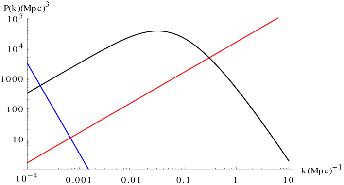
Figure 1: Matter power spectrum for $\Lambda$CDM (black) ${\cal P}_{\Lambda CDM}$ obtained by setting $\delta\sigma=0$. The blue curve represents ${\cal P}_{\Lambda}$ with $n_{\Lambda}=1$ and the red curve with $n_{\Lambda}=5$, with $\mathcal{A}_{\Phi}=\mathcal{A}_{\Lambda}$. We neglect the cross correlation between adiabatic and entropic modes setting ${\cal P}_{\Phi\Lambda}=0$. The total power spectrum is the sum of the black and red curve or the black and the blue one.

Finally, the total matter power spectrum today (at $z=0$) can be expressed in terms of the primordial power spectrum schematically as

$$P(k) \sim\left(\frac{k}{H_{0}}\right)^{4}\left[T_{\Phi}(k)^{2}P_{\Phi}+T_{\Lambda}(k)^{2}P_{\Lambda}+T_{\Lambda}(k)T_{\Phi}(k)\left<\delta_{\Lambda}({\boldsymbol{k}})\,\Phi_{in}({\boldsymbol{k}^{\prime}})\right>\right]$$ (6.15)

$$\equiv{\cal P}_{\Lambda\text{CDM}}(k)+{\cal P}_{\Lambda}(k)+{\cal P}_{\Phi\Lambda}(k)\,$$

where $T_{\Phi}(k)$ and $T_{\Lambda}(k)$ represent the transfer functions for the two possible initial conditions.
The choice of pure adiabatic initial conditions corresponds to set $\delta_{\Lambda}=0$; the matter spectrum is given just by ${\cal P}_{\Lambda\text{CDM}}$ and coincides with the $\Lambda$CDM power spectrum, the black dotted curve in Figure 1. The new contributions stem from ${\cal P}_{\Lambda}$ and ${\cal P}_{\Phi\Lambda}$ and their impact depends on the primordial spectrum for $\delta\sigma$ and the correlation between adiabatic and entropic contributions.
Specifically, while ${\cal P}_{\Lambda\text{CDM}}(k)\sim k^{n_{s}}$ for $k\rightarrow 0$ and ${\cal P}_{\Lambda\text{CDM}}(k)\sim k^{n_{s}-4}$ on small scales (neglecting logarithmic corrections), we have ${\cal P}_{\Lambda}(k)\sim k^{n_{\Lambda}-4}$ always. Contrary to $\Lambda$CDM, where the change of slope is due to modes that entered the horizon at matter domination or at radiation domination, the time-independent nature of $\delta\sigma$ makes its contribution to the matter power spectrum basically monotonic in $k$.
The result is shown in Figure 1 with $n_{s}=1$ for the adiabatic spectral index, while for the entropic index we consider the two cases $n_{\Lambda}=1$ and $n_{\Lambda}=5$ (matching ${\cal P}_{\Lambda\text{CDM}}$ at small or large scales, respectively), and we have chosen the same amplitude $\mathcal{A}_{\Phi}=\mathcal{A}_{\Lambda}$.
From Figure 1 it is clear that unless the size and the shapes of initial perturbations for $\delta\sigma$ are tiny compared with the primordial ones of $\Lambda$CDM, an excess of power at small or large scale will appear, depending on the spectral index $n_{\Lambda}$.

The presence of non-trivial perturbations in the dark sector changes the growth function $D(z)$ defined here as

$$D(z)=\frac{\Delta_{m}(z)}{\Delta_{m}(z_{\text{late}})}\,,\qquad z_{\text{late}}=10\,.$$ (6.16)

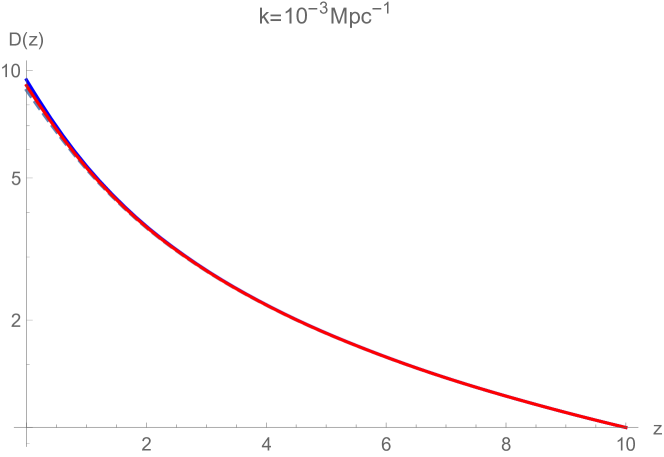
Figure 2: Growth functions.

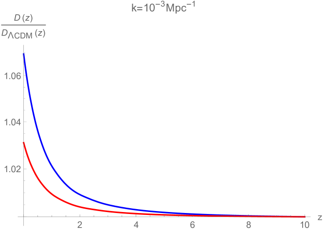
Figure 3: Ratio of the growth factor with $\Lambda$CDM values; same colors as in the figure on the left.

Clearly, in the absence of dark energy the growth function $D(z)$ will grow as $D(z)\sim 1+z$, while the presence of a cosmological constant causes structure to grow less. This is not the case for a $\Lambda$-medium where the growth of structure is enhanced compared to standard $\Lambda$CDM.
Note that for $\Lambda$-media, differently from $\Lambda$CDM, the contribution to the the growth function from the entropy perturbations is generically scale-dependent, and, since $\delta\sigma(k)$ is constant in time, is sensitive to the $k$-dependence of the primordial perturbations specified by the entropic spectral index $n_{\Lambda}$.
The predictions for the growth function is shown in Figure 3, where the black dotted curve shows the case of $\Lambda$CDM, while the blue dashed curve and the red curve show the growth function for $\Lambda$-media with initial conditions $n_{\Lambda}=1$ and $n_{\Lambda}=5$, respectively. The ratio of $D_{\delta_{\Lambda}}$ with the $\Lambda$CDM case is shown in Figure 3.

We leave for a future work a complete numerical analysis suitable for parameter estimation, but clearly the initial spectrum for $\delta\sigma$ is rather constrained from observations.

7 Conclusions

By using the EFT of self-gravitating media, we have shown that there are stable media, protected by symmetries, that feature an exact (non-perturbative) equation of state of the form $p+\rho=0$, and are physically different from a CC. Indeed, adiabatic $\Lambda$-media and, in particular, $\Lambda$-solids and $\Lambda$-special super solids exhibit phonon-like fluctuations which, via Einstein equations, induce non-trivial metric fluctuations. Moreover, the Bardeen potentials and the density contrast of the sub-leading dark matter component $\delta_{m}$ grow as $a^{2}$, in sharp contrast with the case of CC domination, where the Bardeen potentials are decreasing and $\delta_{m}$ is constant. The presence of an intrinsic anisotropic stress induces a strong correlation between the gravitational potentials: $\Psi=-2\;\Phi$ and makes the spin two mode massive. Isentropic $\Lambda$-media are characterised by frozen scalar perturbations, likewise a CC, though spin two perturbations are non-trivial. Indeed, with the exception of $\Lambda$-perfect fluids, the dispersion relation of gravitational waves for stable $\Lambda$-media is the one of a massive particle $\omega=\sqrt{k^{2}+m_{g}^{2}}$. These features can be detectable in future dark energy surveys and gravitational waves experiments. Already the linear matter power spectrum gives a tight constraint on the size of primordial perturbations in the dark energy sector. Some model in which nontrivial dark energy perturbations are present even when $w=-1$ was discussed in [44] in light of the EUCLID mission; here we have given a model independent analysis of stability, the underlying symmetries and the evolution of cosmological perturbations. A detailed analysis of the phenomenological implications of self-gravitating $\Lambda$-media with a parameters estimation will be carried out in a separate work.

Appendix A Mass parameters

The mass parameters $\{M_{b}\}$ are given by

$$\begin{split}&M_{0}=\frac{\phi^{\prime}{}^{2}}{2\,a^{4}\,M_{\text{Pl}}^{2}}\left[a^{2}\left(U_{YY}-2\,U_{X}\right)-4\,a\,\phi^{\prime}\,U_{YX}+4\,\phi^{\prime}{}^{2}\,U_{XX}\right];\\ &M_{1}=\frac{2\,\phi^{\prime}{}^{2}}{M_{\text{Pl}}^{2}}\left[a^{-2}\,U_{X}+\sum_{n=0}^{3}a^{-4-2n}\,U_{y_{n}}\right]\,;\\ &M_{2}=-\frac{2}{M_{\text{Pl}}^{2}}\sum_{m=1}^{3}n^{2}\,U_{\tau_{n}}\,;\\ &M_{3}=\frac{1}{M_{\text{Pl}}^{2}}\left[2\,\sum_{m,n=1}^{3}m\,n\,a^{-2\;(m+n)}\;U_{\tau_{m}\tau_{n}}+2\;\sum_{n=1}^{3}\left(n\;a^{-3-2\;n}\;U_{b\tau_{n}}-\frac{a^{-2\;n}}{2}\;U_{\tau_{n}}\right)+\frac{1}{2\,a^{6}}\;U_{b^{2}}\right]\,;\\ &M_{4}=\frac{\phi^{\prime}}{M_{\text{Pl}}^{2}}\left[\left(\sum_{m,n=1}^{3}a^{1-2n}\;U_{Y\tau_{n}}-\frac{U_{Y}}{2\;a}+\frac{U_{bY}}{2\;a^{4}}\right)-2\;\phi^{\prime}\;\left(\sum_{n=1}^{3}\,a^{-2-2n}\;U_{X\tau_{n}}+\frac{U_{X}}{2\;a^{2}}-\frac{U_{bX}}{2\;a^{5}}\,\right)\right]\,;\end{split}$$ (A.1)

In Minkowski space the mass parameters are obtained form the above expression by setting $a=\phi^{\prime}=1$.

References

- [1] H. Leutwyler. Nonrelativistic effective Lagrangians. Phys. Rev., D49:3033–3043, 1994, hep-ph/9311264.
- [2] H. Leutwyler. Phonons as goldstone bosons. Helv. Phys. Acta, 70:275–286, 1997, hep-ph/9609466.
- [3] D. T. Son. Low-energy quantum effective action for relativistic superfluids. 2002, hep-ph/0204199.
- [4] D. T. Son. Effective Lagrangian and topological interactions in supersolids. Phys. Rev. Lett., 94:175301, 2005, cond-mat/0501658.
- [5] S. Dubovsky, T. Gregoire, A. Nicolis, and R. Rattazzi. Null energy condition and superluminal propagation. JHEP, 03:025, 2006, hep-th/0512260.
- [6] S. Dubovsky, L. Hui, A. Nicolis, and D.T. Son. Effective field theory for hydrodynamics: thermodynamics, and the derivative expansion. Phys. Rev., D85:085029, 2012, 1107.0731.
- [7] G. Ballesteros and B. Bellazzini. Effective perfect fluids in cosmology. JCAP, 1304:001, 2013, 1210.1561.
- [8] G. Ballesteros, D. Comelli, and L. Pilo. Massive and modified gravity as self-gravitating media. Phys. Rev., D94(12):124023, 2016.
- [9] Marco Celoria, Denis Comelli, and Luigi Pilo. Fluids, Superfluids and Supersolids: Dynamics and Cosmology of Self Gravitating Media. JCAP, 1709(09):036, 2017, 1704.00322.
- [10] A. H. Taub. General Relativistic Variational Principle for Perfect Fluids. Phys. Rev., 94:1468–1470, 1954.
- [11] R. L. Seliger and G. B. Whitham. Variational principles in continuum mechanics. Proceedings of the Royal Society of London. Series A, Mathematical and Physical Sciences, 305(1480):1–25, 1968.
- [12] Bernard F. Schutz. Perfect Fluids in General Relativity: Velocity Potentials and a Variational Principle. Phys. Rev., D2:2762–2773, 1970.
- [13] Brandon Carter. Elastic perturbation theory in general relativity and a variation principle for a rotating solid star. Commun.Math.Phys., 30:261–286, 1973.
- [14] B. Carter. Covariant Theory of Conductivity in Ideal Fluid or Solid Media. Lect. Notes Math., 1385:1–64, 1989.
- [15] I. M. Khalatnikov and V. V. Lebedev. Relativistic hydrodynamics of a superfluid liquid. Physics Letters A, 91(2):70–72, 1982.
- [16] S. Endlich, A. Nicolis, and J. Wang. Solid Inflation. JCAP, 1310:011, 2013, 1210.0569.
- [17] Dario Cannone, Gianmassimo Tasinato, and David Wands. Generalised tensor fluctuations and inflation. JCAP, 1501(01):029, 2015, 1409.6568.
- [18] Leila Graef and Robert Brandenberger. Breaking of Spatial Diffeomorphism Invariance, Inflation and the Spectrum of Cosmological Perturbations. JCAP, 1510(10):009, 2015, 1506.00896.
- [19] C. Lin and L. Z. Labun. Effective Field Theory of Broken Spatial Diffeomorphisms. JHEP, 03:128, 2016, 1501.07160.
- [20] Nicola Bartolo, Dario Cannone, Angelo Ricciardone, and Gianmassimo Tasinato. Distinctive signatures of space-time diffeomorphism breaking in EFT of inflation. JCAP, 1603(03):044, 2016, 1511.07414.
- [21] G. Ballesteros, D. Comelli, and L. Pilo. Thermodynamics of perfect fluids from scalar field theory. Phys. Rev., D94:025034, 2016.
- [22] S. L. Dubovsky. Phases of massive gravity. JHEP, 10:076, 2004, hep-th/0409124.
- [23] S. L. Dubovsky, P. G. Tinyakov, and I. I. Tkachev. Massive graviton as a testable cold dark matter candidate. Phys. Rev. Lett., 94:181102, 2005, hep-th/0411158.
- [24] M. Celoria, S. Matarrese, and L. Pilo. Disformal invariance of continuous media with linear equation of state. JCAP, 1702(02):004, 2017, 1609.08507.
- [25] V. A. Rubakov and P. G. Tinyakov. Infrared-modified gravities and massive gravitons. Phys. Usp., 51:759–792, 2008, 0802.4379.
- [26] S. L. Dubovsky, P. G. Tinyakov, and I. I. Tkachev. Cosmological attractors in massive gravity. Phys. Rev., D72:084011, 2005, hep-th/0504067.
- [27] Denis Comelli, Fabrizio Nesti, and Luigi Pilo. Stars and (Furry) Black Holes in Lorentz Breaking Massive Gravity. Phys. Rev., D83:084042, 2011, 1010.4773.
- [28] Michael V. Bebronne and Peter G. Tinyakov. Black hole solutions in massive gravity. JHEP, 04:100, 2009, 0902.3899. [Erratum: JHEP06,018(2011)].
- [29] Diego Blas and Sergey Sibiryakov. Completing Lorentz violating massive gravity at high energies. Zh. Eksp. Teor. Fiz., 147:578–594, 2015, 1410.2408. [J. Exp. Theor. Phys.120,no.3,509(2015)].
- [30] Marco Celoria, Denis Comelli, and Luigi Pilo. Sixth mode in massive gravity. Phys. Rev., D98(6):064016, 2018, 1711.10424.
- [31] V.A. Rubakov. Lorentz-violating graviton masses: Getting around ghosts, low strong coupling scale and VDVZ discontinuity. 2004, hep-th/0407104.
- [32] D. Comelli, F. Nesti, and L. Pilo. Massive gravity: a General Analysis. JHEP, 07:161, 2013, 1305.0236.
- [33] D. Comelli, F. Nesti, and L. Pilo. Nonderivative Modified Gravity: a Classification. JCAP, 1411(11):018, 2014.
- [34] Marco Celoria, Denis Comelli, and Luigi Pilo. Intrinsic Entropy Perturbations from the Dark Sector. 2017, 1711.01961.
- [35] D. Blas, D. Comelli, F. Nesti, and L. Pilo. Lorentz Breaking Massive Gravity in Curved Space. Phys. Rev., D80:044025, 2009, 0905.1699.
- [36] Atsushi Higuchi. Forbidden Mass Range for Spin-2 Field Theory in De Sitter Space-time. Nucl. Phys., B282:397–436, 1987.
- [37] Atsushi Higuchi. Symmetric Tensor Spherical Harmonics on the Sphere and Their Application to the De Sitter Group SO(,1). J. Math. Phys., 28:1553, 1987. [Erratum: J. Math. Phys.43,6385(2002)].
- [38] Stanley Deser and A. Waldron. Stability of massive cosmological gravitons. Phys. Lett., B508:347–353, 2001, hep-th/0103255.
- [39] Luca Grisa and Lorenzo Sorbo. Pauli-Fierz Gravitons on Friedmann-Robertson-Walker Background. Phys. Lett., B686:273–278, 2010, 0905.3391.
- [40] Joao Magueijo and Levon Pogosian. Could thermal fluctuations seed cosmic structure? Phys. Rev., D67:043518, 2003, astro-ph/0211337.
- [41] Joao Magueijo. Near-Milne realization of scale-invariant fluctuations. Phys. Rev., D76:123502, 2007, astro-ph/0703781.
- [42] Yi-Fu Cai, Wei Xue, Robert Brandenberger, and Xin-min Zhang. Thermal Fluctuations and Bouncing Cosmologies. JCAP, 0906:037, 2009, 0903.4938.
- [43] Tirthabir Biswas, Robert Brandenberger, Tomi Koivisto, and Anupam Mazumdar. Cosmological perturbations from statistical thermal fluctuations. Phys. Rev., D88(2):023517, 2013, 1302.6463.
- [44] Luca Amendola et al. Cosmology and Fundamental Physics with the Euclid Satellite. 2016, 1606.00180.