Revisiting the cavity-method threshold for random $3$-SAT

Abstract

A detailed Monte Carlo-study of the satisfiability threshold for random 3-SAT has been undertaken. In combination with a monotonicity assumption we find that the threshold for random 3-SAT satisfies $\alpha_{3}\leq 4.262$. If the assumption is correct, this means that the actual threshold value for $k=3$ is lower than that given by the cavity method. In contrast the latter has recently been shown to give the correct value for large $k$. Our result thus indicate that there are distinct behaviours for $k$ above and below some critical $k_{c}$, and the cavity method may provide a correct mean-field picture for the range above $k_{c}$.

I Introduction

The properties of random $k$-SAT formulae has become one of the most studied intersection points of computer science, mathematics and physics. In this problem we have $n$ Boolean variables $x_{i}$ and we construct a random Conjunctive Normal Form (CNF) formula $F$ by picking $m$ clauses of size $k$ at random. Here each clause is the disjunction, ”OR”, of $k$ literals, and each literal is either a variable or its negation, leading to $2^{k}{n\choose k}$ possible clauses. The formula $F$ is satisfiable if there is an assignment of values to the $x_{i}$:s such that every clause in $F$ becomes True. If $m$ is small then a random formula is with high probability satisfiable and if $m$ is sufficiently large the formula is with high probability not satisfiable. In particular, it is believed, but not known, that there exists constants $\alpha_{k}$ such that for a fixed $\alpha=\frac{m}{n}$ less than $\alpha_{k}$ the probability for satisfiability goes to 1 as $n$ grows, and for $\alpha$ larger than $\alpha_{k}$ it goes to 0. It is known that there exists some $\alpha_{k}(n)$ such that this is true Friedgut and Bourgain (1999), but that the $\alpha_{k}(n)$ is converging to a constant is only known for $k=2$, see e.g., Ref. Chvátal and Reed (1992), where $\alpha_{2}=1$, and sufficiently large fixed $k$ Ding et al. (2015). Using methods from the theory of spin-glasses the values of $\alpha_{k}$, and its existence as a constant, has been calculated non-rigorously Mézard et al. (2002); Mertens et al. (2006), and the results of Ref. Ding et al. (2015) show that this prediction for $\alpha_{k}$ is correct for large enough $k$.

It has also been observed empirically that random CNFs with $\alpha$ close to $\alpha_{k}$ are harder to solve (find a satisfying assignment for or refute) than when $\alpha$ is further away from $\alpha_{k}$. It has repeatedly been speculated that this peak in the hardness of the formulae is related to the clustering properties of the set of solutions, as a function of $\alpha$. However, here there are no corresponding rigorous hardness results, and since it is now known that polynomial time solvable problems like random XOR-SAT have the same type of clustering Achlioptas and Molloy (2015); Ibrahimi et al. (2015) this connection is no longer thought be straightforward. The solution clustering in itself has been verified for large $k$ Achlioptas (2008). Another early product of applying the cavity method to random $k$-SAT is the survey-propagation algorithm. This algorithm empirically demonstrated a good ability to find solutions to satisfiable random $k$-SAT instances close to the satisfiability threshold and it was conjectured that it would work for all densities up to the threshold, unlike other randomized algorithms which are known to fail before reaching the threshold. However, this has now been rigorously proven to not be the case, both for the simpler belief-propagation method Coja-Oghlan (2017) and the full survey-propagation method Hetterich (2016). In Coja-Oghlan (2017) the reason for this is discussed in detail, and one of the reasons is that the cavity method makes some too simple assumptions on the correlations in the model, for densities close to the threshold.

Since the existence of $\alpha_{k}$ has been established for large $k$, and the related threshold is understood in quite some detail for $k=2$, our aim has been to provide an improved test of the prediction for $k=3$. Before the predictions from the cavity method arrived several sampling studies of the thresholds were made, for many values of $k$, but after the predictions were made no large scale study of these predictions has been undertaken. One obvious reason for this is that the computer time needed for such studies grows exponentially with the number of variables, and in order to get the required accuracy a large number of samples is needed. The latter is especially important since many of the scalings used to analyse the data in the earlier simulation papers were later ruled out by rigorous mathematical results Wilson (2002), thereby invalidating the method behind those results.

We have sampled the random 3-SAT problem both with more variables than in earlier studies, up to $n=375$ and a far larger number of samples per density. In earlier papers typically a few thousand samples were used, while for most values of $n$ we have several millions instead. Our main aim has been to provide an upper bound on the value of $\alpha_{3}$ and under a mild monotonicity assumption we find an upper bound of $\alpha_{3}\leq 4.262$. This value is clearly smaller than the cavity-method prediction $\alpha_{*}=4.26675$ Mertens et al. (2006), but closer to the earlier Crawford and Auton (1996) simulation estimate which arrived at $4.258$, using an invalid scaling. It has already been noted Krz̧akała et al. (2007) that in terms of the solutions space geometry the case $k=3$ differs from $k\geq 4$, indicating that small values of $k$ might be exceptional, and we will discuss possible reasons for the deviation of the numerical prediction $\alpha_{*}$ from the actual value.

II Sampling details

In order to estimate the 3-SAT threshold we have sampled the random 3-SAT model for $n=4$, $8$, $16$, $32$ and $n=25,50,\ldots,375$. We also attempted sampling for larger $n$ but there the sampling was so slow that we could not generate the amount of data needed in order to control the sampling noise. We used the MiniSAT solver to generate our data Eén and Sörensson (2004). For each value of $n$ we produced random formulae with a fixed number of clauses $m$, for a range of values of $m$.

The number of samples were as follows, for $n=100,\ldots,200$ we have $N=4\times 10^{6}$ samples, for $n=225,\ldots,300$, $N=10^{6}$, for $n=325$, $N=5\times 10^{5}$, for $n=350$, $N=10^{5}$, and for $n=375$, $N=1.4\times 10^{4}$. In each case we used densities in the interval $[4.2,4.3]$. For $n=350$ and $n=375$ we attempted to compensate for the smaller number of samples by slightly increasing the number of densities, but as we will see these two cases would still require more samples in order to give sharp results.

We also sampled 2-SAT and 4-SAT, for $k=2$ we collected $10^{4}$ samples for each size and density, and for $k=4$ we collected at least $10^{4}$ for each size and density for $n=50$, $75$, $100$, $125$. For 2-SAT we also used a data set produced by David Wilson Wilson . This has $10^{4}$ samples per size for $n=2^{t}$ where $t=1,\ldots,20$. The data from Wilson is produced in a different way from our own samples. Wilson starts with an empty formula $F_{0}$ and step by step produces a new formula $F_{t}$ from $F_{t-1}$ by adding a random clause to $F_{t-1}$, stopping when $F_{t}$ is unsatisfiable. The random formula $F_{t}$ is distributed in exactly the same way as a random formula with $n$ variables and $t$ clauses. For $k=2$ this sampling method is efficient due to the existence of a linear time algoritm for 2-SAT, but for larger $k$ the standard method, which we have used, is more efficient.

III The threshold for random 3-SAT

In order to estimate the value of $\alpha_{3}$ we have focused on the value $\alpha(n,p)$ where the probability of being satisfiable is equal to $p$, and in particular $p=\frac{1}{2}$. The sharp threshold result of Ref. Friedgut and Bourgain (1999) shows that, if the limit $\alpha_{3}$ exists, the value $\alpha(n,p)$ will converge to $\alpha_{3}$ for any fixed value $p$. However, the rate of convergence may depend on $p$.

The quantity $\alpha(n,1/2)$ has been used in several earlier studies, e.g., Refs. Selman and Kirkpatrick (1996); Crawford and Auton (1996), where the approach has been to fit a function of the form $an+bn^{\beta}$ to the estimated values of $\alpha(n,1/2)$ for some range of values of $n$. In Ref. Crawford and Auton (1996) the value $\beta=-2/3$ was found to give a good fit to the data. However, in Ref. Wilson (2002) it was proven that there can exist at most one value $p$ such that $\alpha(n,p)=\alpha_{3}+o(n^{-\frac{1}{2}})$ and as pointed out in Ref. Wilson (2002) the experimental data indicates that the unique such value for $p$, if it exists at all, is not $\frac{1}{2}$. Hence a data fit of the type used in Refs. Selman and Kirkpatrick (1996); Crawford and Auton (1996) is unlikely to be valid, and if we change the value of $p$ by any amount it is guaranteed that the form of the fitted function is valid for at most one of the two values for $p$, no matter how small the difference between them are.

In order to demonstrate the discussed problem we look at the case $k=2$, where we both have data for extremely large $n$ Wilson and rigorous results Bollobás et al. (2001) on the threshold. In Fig. 1 we see the estimated values of $\alpha(n,1/2)$ as a function of $1/n$ for a range of $n$ similar to that used for $k=3$. This graph was produced in the way which we will discuss for 3-SAT in the next section. Here we know that $\alpha=1$ and the scaling exponent for $1-\alpha(n,1/2)$ is $1/3$ Bollobás et al. (2001). Nonetheless even a simple second degree polynomial gives a reasonable fit to the data for $n\leq 250$. Next, in Fig. 2 we see the same quantity but now for $n$ from $4$ up to $2^{20}$ and with a fitted function based on the correct scaling exponent. Here the value of $\alpha(n,1/2)$ was produced by finding the median stopping time in Wilson’s data. The median stopping time is identical to the number of clauses $m$ given by $\lceil n\alpha(n,1/2)\rceil$, so the two methods give easily comparable data. The good fit of the polynomial in the first figure is entirely due to the small values of $n$ and has nothing to do with the correct asymptotics. So, for the case $k=2$ one can clearly be misled by small values of $n$.

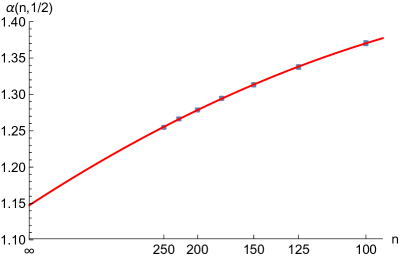
Figure 1: (Colour on-line) For $k=2$, $\alpha(n,1/2)$ versus $n$ for $n=100,125,\ldots,250$ and the fitted polynomial (red curve) $1.15+30.1x-785x^{2}$, where $x=1/n$. Error bars are smaller than the points.

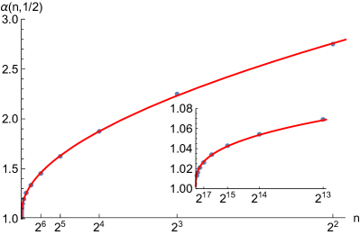
Figure 2: (Colour on-line) For $k=2$, $\alpha(n,1/2)$ versus $n$ for $n=2^{2},2^{3},\ldots,2^{20}$ and the fitted curve (red) $1.00+1.21x^{1/3}+2.51x^{2/3}$, where $x=1/n$. Error bars are smaller than the points.

We now proceed to our data for $k=3$. In order to estimate the value of $\alpha(n,1/2)$ we fitted, for each $n$, a line to the interval where the probability $p$ for being satisfiable is in the range $|p-\frac{1}{2}|\leq 0.15$, and then found the point where this line was equal to $1/2$, using this as our estimate for $\alpha(n,1/2)$. We also tried polynomials rather than lines but in this interval the curve is so close to linear that higher degree polynomials provided no discernible improvement. In Fig. 3 we see the sampled data for the larger $n$ together with the fitted lines.

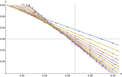
Figure 3: (Colour on-line) For $k=3$, the probability $p$ of being satisfiable versus $\alpha$, together with fitted lines for $n=100,\ldots,375$ (downwards at $\alpha=4.30$). Dashed lines at $\alpha=\alpha_{*}$ (vertical) and $p=1/2$ (horisontal).

We estimate $\alpha(n,1/2)$ for $n=100,125,\ldots,375$ as, respectively,

$$4.2897,4.2788,4.2725,4.2687,$$

$$4.2661,4.2645,4.2633,4.2626,$$

$$4.2621,4.2618,4.2619,4.2616$$

We have considered three sources for errors in these estimates, the sampling noise, the degree of the polynomial fitted to the data, and the choice of density values used in the fit. The dominant error turns out to be the sampling noise. Since we have perfectly independent samples we can do a correct error estimate for the estimate by using bootstrap in the form of resampling, i.e., obtaining estimates on different subsets of the data and finding the standard deviation of the estimate under resampling. All $n\leq 325$ give similar values for the error estimate and in each case it is at most $0.000176$, for $n=350$ we get $0.00027$ and for $n=375$ we get $0.0011$. In Fig. 4 the error bars give the exact error estimate for each $n$. As expected the size of the error closely follows the number of samples.

We also considered the stability under using a polynomial of higher degree than 1 in the fit to the data. Using polynomials up to degree 4 this error turns out to be smaller than the sampling error, and is in fact decreasing with $n$, indicating that the curve becomes more and more linear in the given interval as $n$ grows. We saw a similar behavior when we used different subsets of the density values in the fit, here the error for $n=375$ was less than 1% of the sampling error.

The $\alpha(n,1/2)$-values are shown in Fig. 4. Again we see an almost linear behavior for small $n$, as the inset picture shows, and then for the largest $n$ the points seem to level out. For the last two points noise becomes noticable due to the too small number of samples for those $n$. The points in Fig. 4 can be well approximated by a second degree polynomial, but, as mentioned before, from Ref. Wilson (2002) we know that this is not a valid scaling. In fact, we would expect the curve to behave as a suitable root of $1/n$, just like in Fig. 1, but we clearly do not have large enough values of $n$ here to see the range where the asymptotic behavior becomes dominant.

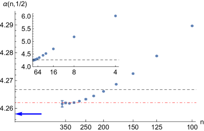
Figure 4: (Colour on-line) For $k=3$, $\alpha(n,1/2)$ versus $n$ for $n=100,125,\ldots,375$. Black dashed line at $\alpha_{*}=4.26675$, red dot-dashed line at our upper bound $4.262$, blue arrow at estimate $4.258$ Crawford and Auton (1996). Inset shows zoomed-out version, for $n\geq 4$, dashed line at $\alpha_{*}$.

We find further evidence for the fact that we have too small values of $n$ if we look at the width of the scaling window. If we look at $\alpha(n,0.65)-\alpha(n,0.35)$ we know from Ref. Wilson (2002) that this width cannot be $o(n^{-1/2})$, but in a log-log plot of this, as shown in Fig. 5, we see that we get the fitted line $1.0802-0.6255x$. This gives a scaling of $n^{-0.625}$, which is ruled out Wilson (2002). The exponent $0.625$ is smaller than the $2/3$ found in Refs. Selman and Kirkpatrick (1996); Crawford and Auton (1996). This could be due to the larger values of $n$ used here and might indicate that we are at least getting closer to the size range where the asymptotic scaling becomes visible.

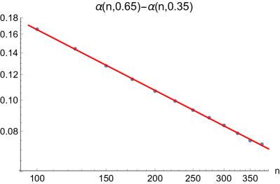
Figure 5: For $k=3$, log-log plot of $\alpha(n,0.65)-\alpha(n,0.35)$ versus $n$ for $n=100,125,\ldots,375$ and the fitted line (red) $1.0802-0.6255x$, with $x=\ln n$.

With this in mind we find that one cannot give a credible estimate for $\alpha_{3}$ with any accuracy based on this range of $n$ and have instead taken the more modest aim of providing an upper bound on $\alpha_{3}$. In order to do this we have taken as our working assumption that $\alpha(n,1/2)$ is in fact monotone in $n$, something we believe to be true for large enough $n$.

Conjecture.

For any $k\geq 2$ there exists an $n_{0}$ such that for $n\geq n_{0}$ the value of $\alpha(n,1/2)$ is decreasing in $n$.

There are several reasons for believing that this type of monotonicity should hold, and that $n_{0}$ will also be small. On one hand this is a common occurrence for probabilistic combinatorial problems, and it is also seen in many coupon-collector problems.

A coupon-collector problem has some base set $X$ and at each time step $i$ a random subset $Y_{i}$ of $X$ is chosen with replacement, according to some distribution for the $Y_{i}$, until all elements of $X$ are covered by at least one $Y_{i}$. That random $k$-SAT can be viewed as a coupon-collector problem is a folklore result and has been used in several published papers, e.g., Refs. Zito (1999); Kaporis et al. (2001). Here the base set $X$ is the hypercube $Q_{n}$ consisting of all binary strings of length $n$, and each random set $Y_{i}$ is a random subcube of dimension $n-k$, corresponding to the solutions ruled out by a clause of size $k$. A $k$-SAT formula is unsatisfiable if the corresponding collection of sets $Y_{i}$ cover all elements of the hypercube $Q_{n}$. As mentioned in connection with Wilson’s data the value $\alpha(n,1/2)$ corresponds exactly to the median stopping time of the coupon-collector process. For the simplest coupon-collector problem the median, as well as the full distribution of the stopping time, was derived in Ref. Erdős and Rényi (1961), and after normalization to make it converge, it does indeed decrease to it’s asymptotic value. General coupon-collector problems have been studied, e.g., in Ref. Falgas-Ravry et al. (2016) where $k$-SAT is also discussed, and for many such examples the type of monotonicity conjectured above can be proven. In fact we know of no natural examples where this type of monotonicity is known to fail, but there is no general monotonicity result which includes the case of $k$-SAT for fixed $k$.

A second reason for expecting both monotonicity and a low value of $n_{0}$ comes from the seminal results of Ref. Chvátal and Szemerédi (1988). There a rigorous analysis of the structure of a random unsatisfiable $k$-SAT formula $F$ was undertaken for all densities $\alpha$, not only for values above the threshold. One of the main results is that there exists a function $g_{k}(\alpha)$ such that the smallest unsatisfiable sub-formula of $F$ has at least $ng_{k}(\alpha)$ variables, and this function $g_{k}(\alpha)$ is decreasing with $\alpha$. So, the unsatisfiability of $F$ is explained by the appearance of an unsatisfiable sub-formula $F^{\prime}$ which has linear size, but the relative size is smaller for higher densities $\alpha$. However, the set of unsatisfiable formulae on $ng_{k}(\alpha)$ variables is more restricted for small $n$ than for larger $n$, since there are more ways of realizing such a formula for larger $n$, and likewise is more restricted the larger $g_{k}(\alpha)$ is. Hence one should expect the set of such formulae to be closer to its asymptotic behavior for small values of $g_{k}(\alpha)$, i.e, for large densities $\alpha$. This would then mean that for larger densities we see a faster convergence to the asymptotic probability of satiability, also indicating that $\alpha(n,1/2)$ should move to the left. Indeed, the point $\alpha(n,1/2)$ also corresponds to the density where the median number of unsatisfiable sub-formulae in $F$ is at least 1, and if we add as little as $O(\ln(n))$ the expected number of unsatisfiable sub-formulae of size at least $ng_{k}(\alpha)$ in $F$ will be at least polynomial in $n$.

For $k=2$ the conjecture agrees with both data, as shown in Fig. 2, and with what one would expect from the mathematical results Chvátal and Reed (1992); Bollobás et al. (2001), even though this is not explicitly proven in the latter. Our sequence of values for $\alpha(n,1/2)$ is compatible with this assumption with the exception for the value at $n=350$, but a closer examination of the data for the two largest values of $n$ shows that those estimates are too noisy for the needed accuracy. Under the monotonicity assumption and a very pessimistic view of the sampling errors we can then confidently give the bound

$$\alpha_{3}\leq 4.2620.$$

In Fig. 4 we see values of $\alpha(n,1/2)$ for $n\geq 100$ together with lines indicating the cavity-method prediction $\alpha_{*}=4.26675$, our asymptotic upper bound, and an arrow marking the early estimate $4.258$ from Ref. Crawford and Auton (1996).

IV Discussion

As we have seen, our upper bound for $\alpha_{3}$ is incompatible with the cavity-method prediction from Refs. Mézard et al. (2002); Mertens et al. (2006). We note that our estimate for $\alpha(200,1/2)$ is already below the predicted asymptotic value, that is in the range for $n$ where we have $N=4\times 10^{6}$ samples per density so we are confident that our estimate is accurate.

One explanation for the contradiction between our bound and $\alpha_{*}$ could of course be that $\alpha(n,1/2)$ is not monotone, but this would require a strong, and in our opinion surprising, finite-size correction to the observed behavior, which would also differ from what we see at $k=2$. In Fig. 6 we show a plot of $\alpha(n,1/2)$ for $k=4$, for $n=50$, $75$, $100$, $125$ and we once again see a monotone decrease with $n$. Here the values (estimated to $10.000$, $9.962$, $9.945$, $9.941$, respectively) stay above the cavity-method prediction $9.931$ for $k=4$, but the values of $n$ are even smaller than for $k=3$.

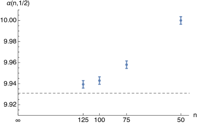
Figure 6: For $k=4$, $\alpha(n,1/2)$ versus $n$ for $n=50$, $75$, $100$, $125$. Dashed line at cavity-method estimate $\alpha_{*}=9.931$.

Another explanation could lie in the numerical determination of $\alpha_{*}$ in Ref. Mertens et al. (2006). In that paper a set of equations for $\alpha_{*}$ is derived, but they are in terms of an optimum over a set of distribution functions which are not explicitly known. In order to find $\alpha_{*}$ they perform a numerical search over a quite complicated search space and it is possible that this search has in fact not found a correct optimum. In an earlier paper Mézard et al. (2002) the smaller value $4.256$ was stated, but then changed Mertens et al. (2006) after it was found that the numerical procedure was sensitive to the type of random number generator used in the search. However, this problem would have to be unusually sensitive if numerical errors has led to incorrect optima both above and below the actual value.

The third and perhaps most intriguing possibility is that the cavity method itself, as used in Refs. Mézard et al. (2002); Mertens et al. (2006), does in fact not give a correct prediction for $\alpha_{3}$. We know from Ref. Ding et al. (2015) that the cavity method does give the correct value for $\alpha_{k}$ for large enough $k$, but those authors have stated that they do not think that their proof can be extended all the way down to $k=3$. It has also been found Krz̧akała et al. (2007) that the cavity method predicts that other thresholds, which describe properties of the set of solutions to a satisfiable $k$-SAT formula, behave differently for $k=3$ and $k\geq 4$. In the former case some of the generally distinct thresholds coincide. Those authors also found that the analysis of the method would require changes for $k=3$, thus indicating that for the cavity method itself the case $k=3$ is distinct.

In combination with our results this leads to a picture where the cavity method may provide the correct mean-field type behavior for $k$ above some critical $k_{c}$, leaving a few distinct cases for lower $k$, much in analogy with the high and low-dimensional behavior for classical phase transitions, like random walks, percolation and the Ising model. In either of the two latter cases the well known prediction $\alpha_{*}=4.26675$ is not correct and a further investigation of the case $k=3$ for random $k$-SAT seems worthwhile, both from a mathematical and a physical point of view.