Spectral Methods for Coupled Channels with a Mass Gap

Abstract

We develop a method to compute the vacuum polarization energy for coupled scalar fields with different masses scattering off a background potential in one space dimension. As an example we consider the vacuum polarization energy of a kink-like soliton built from two real scalar fields with different mass parameters.

I Introduction

Many non-linear field theories allow for localized field configurations that are stable due to their topological properties or, when they possess non-trivial conserved quantum numbers, because they are energetically favored over trivial configurations with the same quantum numbers. These configurations are frequently called solitons, even though strictly speaking they are merely solitary waves Ra82 . In specific cases, the energetical stabilization mechanism requires the inclusion of quantum corrections Farhi:2000ws ; Weigel:2010zk . These so-called vacuum polarization energies (VPEs) emerge as the renormalized sums of the shifts of the zero point energies for the quantum fluctuations about the soliton. Of course, computing the VPE for a soliton configuration is also an interesting subject even before addressing the stabilization issue. In that calculation a major obstacle is the appearance of ultra-violet divergences which are characteristic for quantum field theories. Spectral methods Graham:2009zz have proven efficient at handling these divergences, by computing the VPE from scattering data of the potential generated by the soliton and identifying the divergences from the corresponding Born series. The latter is then expressed as a series of Feynman diagrams that are regularized and renormalized by techniques common in perturbative quantum field theory. Still, the full calculation is exact and the Born approximation serves only as a mechanism for isolating potentially divergent contributions in a tractable form.

Spectral methods, i.e. the use of quantum scattering calculations, have a long history in the context of VPEs. The foundation to this approach was formulated by Schwinger Schwinger:1954zz . Early applications include the renowned work published in Ref. Dashen:1974cj and various examples compiled in Ref. Ra82 . In our treatment the Jost function is central, however, the VPE can also be computed from scattering formulations of the Green’s functions Baacke:1989sb ; Graham:2002xq . Alternatively, the fluctuation determinant is directly computed (or estimated) within heat kernel methods Bordag:1994jz in conjuction with $\zeta$-function renormalization Elizalde:1996zk (for the present investigation the heat kernel calculations of Refs. AlonsoIzquierdo:2012tw ; AlonsoIzquierdo:2003gh are particularly relevant), the world line formalism Gies:2003cv , derivative expansions Aitchison:1985pp , or the Gel’fand-Yaglom method Gelfand:1959nq ; just to name a few other techniques. Many of them have been motivated by research on the famous Casimir effect Casimir:1948dh . For further details (and many more references) on these calculations we refer to pertinent reviews and text books Mostepanenko:1997sw ; Graham:2009zz . For the VPE of a single quantum fluctuation off smooth backgrounds in one space dimension these methods produce consistent results. This is mainly due to the fact that merely a single, local Feynman diagram must be renormalized. However, in higher dimensional cases, the approximative character of some of these approaches causes deviations. Deviations between different approaches have also been observed for the VPE in one-dimensional models when un-conventional field configurations are involved as e.g. for the $\phi^{6}$ model kink AlonsoIzquierdo:2011dy .

Here we extend the spectral method formalism to the multi-threshold case. We begin from $F(k)$, the Jost function, or in a multi-channel scattering problem the Jost determinant, where $k$ is the momentum of the scattering wave-function. Several analytic properties of $F(k)$ will be essential: (i) it must be analytic in the upper half complex $k$-plane; (ii) it must have simple zeros for purely imaginary $k={\rm i}\kappa_{i}$ representing the bound state solutions; and (iii) its phase, i.e. the physical scattering phase shift, must be anti-symmetric for real $k$: $F(-k)=F^{\ast}(k)$. With mild conditions on the background potential these properties are well established even in problems with several independent momentum like variables $k_{1},k_{2},\ldots$. That is, a Jost function can be constructed that reflects these properties as a function of $k_{1}$ with $k_{2},\ldots$ fixed or, alternatively, as a function of $k_{2}$ with $k_{1},\ldots$ fixed Newton:1982qc ; Chadan:1977pq .

The situation changes drastically when the momentum variables are not independent as is the case when coupled particles with different masses scatter off a background potential. As a prototype example, we consider two particles with masses $m_{1}$ and $m_{2}$. Since the background potential is static, the energy of the fluctuations is conserved. Using relativistic dispersion relations, the momenta are therefore related as

$$k_{1}^{2}+m_{1}^{2}=k_{2}^{2}+m_{2}^{2}\,.$$ (1)

We adopt the convention $m_{1}\leq m_{2}$ so that $k_{1}$ is real for the physical scattering process, and treat $k_{1}$ as the independent momentum variable. This choice induces a square root dependence of $k_{2}$ on $k_{1}$ which may lead to additional branch cuts in the complex $k_{1}$ plane. Within the gap, $k_{1}^{2}<m_{2}^{2}-m_{1}^{2}$, the second momentum variable becomes complex and, at least in the lower complex half plane, analytic properties are most likely lost. Within that gap it is also important to ensure that the wave-function of the heavier particle decreases exponentially towards spatial infinity. In view of these obvious obstacles it is the main objective of the present investigation to establish a comprehensive scattering formalism for the VPE in this case, where we generalize Eq. (1) to complex momenta such that the above required properties of the Jost function $F(k_{1})$ are maintained.

There are additional technical advantages of analytically continuing to complex momenta. Rotating the momentum integral over the phase shift onto the imaginary axis automatically includes the bound state contribution to the VPE and they need not be explicitly constructed. Nevertheless we will do so in certain cases to verify the analytic properties of $F(k_{1})$. Additionally, at threshold, $k_{2}=0$, the phase shift typically exhibits cusps that are difficult to handle numerically. This problem is avoided on the imaginary axis, as is the one of numerically constructing a phase shift as a continuous function of $k_{1}$ from the phase of the determinant of the scattering matrix without $2\pi$ jumps. Furthermore, as we will discuss below, for $m_{1}\neq m_{2}$ a consistent formulation of the no-tadpole renormalization condition is problematic when the VPE is formulated as an integral over real momenta.

The paper is organized as follows. In Section II we explain the problem and relate $k_{1}$ and $k_{2}$ such that the scattering problem is well-defined along the real $k_{1}$ axis and an analytic continuation to the upper half complex $k_{1}$ plane is possible. In Section III, we then define the Jost determinant for a spatially symmetric potential and demonstrate the necessary analytic properties of this determinant by numerical simulations. In Section IV we generalize this approach to a potential with mixed reflection symmetry similar to parity in the Dirac theory. In Section V we formulate the VPE in terms of an integral of the Jost determinant along the positive imaginary momentum axis. In Section VI we apply this spectral method to the soliton model with two real scalar fields proposed in Ref. Bazeia:1995en in Section VI to investigate whether the classical degeneracy of soliton configurations is broken by quantum corrections. Our results provide the exact one-loop VPEs, extending previous calculations that used the fluctuation spectrum to confirm stability of these solutions Boya:1989dn ; Bazeia:1996np ; Bazeia:1997zp ; Bazeia:1998zv ; Veerman:1999kx . A short summary is given in Sec. VII. Technical issues are discussed in two appendixes. In Appendix A we verify the analytical structure of the Jost determinant by numerically simulating contour integrals and in Appendix B we investigate the VPE for the particular case of two un-coupled particles with a mass gap.

II Multi-threshold scattering

We consider a field theory in one space dimension with two scalar fields $\Phi_{1}$ and $\Phi_{2}$. We write the Lagrangian in terms of the field potential $U(\Phi_{1},\Phi_{2})$

$$\mathcal{L}=\frac{1}{2}\sum_{i=1}^{2}\left[\partial_{\mu}\Phi_{i}\partial^{\mu}\Phi_{i}-m_{i}^{2}\Phi_{i}^{2}\right]-U(\Phi_{1},\Phi_{2})\,,$$ (2)

and assume that the classical field equations produce a localized static solution $\Phi_{\rm sol}(x)=(\Phi_{\rm sol,1}(x),\Phi_{\rm sol,2}(x))$. Fluctuating fields with frequency $\omega$ are then introduced as $\Phi(x,t)=\Phi_{\rm sol}(x)+{\rm e}^{-{\rm i}\omega t}\left(\phi_{1}(x),\phi_{2}(x)\right)$. For simplicity, the frequency dependence of the fluctuations $\phi_{i}(x)$ is not made explicit. To harmonic order these fluctuations are subject to the wave equation

$$-\frac{d^{2}}{dx^{2}}\begin{pmatrix}\phi_{1}\cr\phi_{2}\end{pmatrix}=\begin{pmatrix}k_{1}^{2}&0\cr 0&k_{2}^{2}\end{pmatrix}\begin{pmatrix}\phi_{1}\cr\phi_{2}\end{pmatrix}-V(x)\begin{pmatrix}\phi_{1}\cr\phi_{2}\end{pmatrix}\,,$$ (3)

where the diagonal momentum matrix arises from the dispersion $\omega^{2}=k_{1}^{2}+m_{1}^{2}=k_{2}^{2}+m_{2}^{2}$ and $V(x)$ is the $2\times 2$ potential matrix that couples the two fluctuating fields via the soliton background

$$V_{ij}(x)=\frac{1}{2}\,\frac{\partial^{2}U(\Phi_{1},\Phi_{2})}{\partial\Phi_{i}\partial\Phi_{j}}\Big{|}_{\Phi=\Phi_{\rm sol}}\,.$$ (4)

At this point we assume $V(x)=V(-x)$, but we will also discuss a different scenario in Section IV. Note that for investigating the analytic properties of scattering data it is not necessary that the potential arises from a soliton model.

As mentioned in the introduction, we take $k=k_{1}$ to be the independent momentum variable. Then the dependent momentum variable $k_{2}=k_{2}(k)$ must have (at least) three important properties:

1. For any real $k$ within the gap, $k^{2}<m_{2}^{2}-m_{1}^{2}$, the dependent momentum $k_{2}$ is imaginary with a positive imaginary part, so that ${\rm i}k_{2}\leq 0$ leads to a localized wave-function in the closed channel.

2. For any real $k$ outside the gap, $k^{2}\geq m_{2}^{2}-m_{1}^{2}$, the dependent momentum $k_{2}$ is also real and $k\to-k$ must imply $k_{2}\to-k_{2}$. This will ensure $F(-k)=F^{\ast}(k)$.

3. If ${\sf Im}(k)\geq 0$ then we must also have ${\sf Im}(k_{2})\geq 0$ such that both momenta are in their respective upper half complex planes.

Properties 1. and 2. seem contradictory because the first one does not allow for a sign change of $k_{2}$ while the second one requires it. We will now show that

$$k_{2}=k_{2}(k)\equiv k\sqrt{1-\frac{m_{2}^{2}-m_{1}^{2}}{\left[k+{\rm i}\epsilon\right]^{2}}}\qquad{\rm with}\qquad\epsilon\to 0^{+}$$ (5)

indeed possesses these properties. Property 2. is obvious because outside the gap the real part of the radical is positive and the ${\rm i}\epsilon$ prescription that moves the pole into the lower half plane can be ignored. Within the gap, $k^{2}<m_{2}^{2}-m_{1}^{2}$, we expand in $\epsilon$ with careful attention to the sign of its coefficient, yielding

$$k_{2}(k)=k\sqrt{1-\frac{m_{2}^{2}-m_{1}^{2}}{k^{2}}+{\rm i}\,{\rm sign}(k)\epsilon}=k{\rm i}\,{\rm sign}(k)\sqrt{\frac{m_{2}^{2}-m_{1}^{2}}{k^{2}}-1}=+{\rm i}\sqrt{m_{2}^{2}-m_{1}^{2}-k^{2}}\,,$$ (6)

satisfying Property 1. above. Property 3. is established by introducing $k=s+{\rm i}t$ with real $s$ and $t$ in the relation between $k$ and $k_{2}$, generalizing Eq. (6)

$$k_{2}=(s+{\rm i}t)\sqrt{1-(m_{2}^{2}-m_{1}^{2})\frac{s^{2}-t^{2}}{(s^{2}+t^{2})^{2}}+2{\rm i}\frac{st(m_{2}^{2}-m_{1}^{2})}{(s^{2}+t^{2})^{2}}}\,.$$ (7)

We define $X$ and $Y$ such that

$$\sqrt{1-(m_{2}^{2}-m_{1}^{2})\frac{s^{2}-t^{2}}{(s^{2}+t^{2})^{2}}+2{\rm i}\frac{st(m_{2}^{2}-m_{1}^{2})}{(s^{2}+t^{2})^{2}}}=(X+{\rm i}\,{\rm sign}(st)Y)\,.$$ (8)

The square root halves the phase of any complex number, i.e. it maps phases in $[-\pi,\pi]$ to $[-\pi/2,\pi/2]$, implying $X\geq 0$. Also the sign of the imaginary part does not change when taking the square root, so that $Y\geq 0$ as well. From this it follows that ${\sf Im}(k_{2})=|s|{\rm sign}(t)Y+tX\geq 0$ when $t\geq 0$, which is the third required property.

With these momentum variables, we are now prepared to parameterize the Jost solution as a matrix-valued function. Its columns contain the two functions $\phi_{1}$ and $\phi_{2}$ subject to specific boundary conditions: Outside the gap, the rows refer to the two independent boundary conditions of out-going plane waves of the individual particles at positive spatial infinity. Inside the gap, the second boundary condition parameterizes a localized wave-function in the closed channel. To this end we apply the differential operator from Eq. (3) to

$$F(k,x)=Z(k,x)\begin{pmatrix}{\rm e}^{{\rm i}kx}&0\cr 0&{\rm e}^{{\rm i}k_{2}(k)x}\end{pmatrix}$$ (9)

and obtain the second order differential equation for the coefficient matrix function

$$Z^{\prime\prime}(k,x)=-2Z^{\prime}(k,x)D(k)+M^{2}Z(k,x)-Z(k,x)M^{2}+V(x)Z(k,x)\,,$$ (10)

where primes denote derivatives with respect to the spatial coordinate while

$$D(k)={\rm i}k\begin{pmatrix}1&0\cr 0&\sqrt{1-\frac{m_{2}^{2}-m_{1}^{2}}{\left[k+{\rm i}\epsilon\right]^{2}}}\end{pmatrix}\qquad{\rm and}\qquad M^{2}=\begin{pmatrix}m_{1}^{2}&0\cr 0&m_{2}^{2}\end{pmatrix}$$ (11)

denote space-independent diagonal matrices. The boundary conditions then translate into $\lim_{x\to\infty}Z(k,x)=\mbox{{\sf 1}\mbox{}\rule{0.39993pt}{6.6736pt}\mbox{\hskip 1.00006pt}}$ and $\lim_{x\to\infty}Z^{\prime}(k,x)=0$.

Since Eq. (3) is real, the physical scattering solutions are linear combinations of $F(k,x)$ and $F^{\ast}(k,x)=F(-k,x)$. With the assumption that $V(-x)=V(x)$ these solutions decouple into symmetric and anti-symmetric channels

$$\Phi_{S}(k,x)=F(-k,x)+F(k,x)S_{S}(k)\qquad{\rm and}\qquad\Phi_{A}(k,x)=F(-k,x)+F(k,x)S_{A}(k)\,,$$ (12)

where $S_{S}$ and $S_{A}$ are the scattering matrices that are obtained from the boundary conditions $\Phi_{S}^{\prime}(k,0)=0$ and $\Phi_{A}(k,0)=0$ in the respective channels. For the VPE we merely require the sum of the eigenphase shifts given by the (logarithm of the) determinant of the scattering matrices. Hence we write

$${\rm det}\left[S_{S}(k)\right]={\rm det}\left[F^{-1}_{S}(k)F_{S}(-k)\right]\qquad{\rm and}\qquad{\rm det}\left[S_{A}(k)\right]={\rm det}\left[F^{-1}_{A}(k)F_{A}(-k)\right]$$ (13)

with the Jost matrices

$$F_{S}(k)=\lim_{x\to 0}\left[Z^{\prime}(k,x)D^{-1}(k)+Z(k,x)\right]\qquad{\rm and}\qquad F_{A}(k)=\lim_{x\to 0}Z(k,x)\,.$$ (14)

In the symmetric channel, alternative definitions of the Jost matrix $F_{S}(k)$ with different factors of $D(k)$ lead to the same determinant of $S_{S}$, because $D^{\ast}(k)=D(-k)$. This ambiguity is removed by demanding that $F_{S}(k)$ be the unit matrix for $V\equiv 0$, which is equivalent to requiring $\lim_{k\to\infty}F_{S}(k)=\mbox{{\sf 1}\mbox{}\rule{0.39993pt}{6.6736pt}\mbox{\hskip 1.00006pt}}$. The factor of $D(k)$ as in Eq. (14) adds multiples of $\pi$ to to the phase shift when $k^{2}\leq m_{2}^{2}-m_{1}^{2}$. In Appendix B we show that these multiples of $\pi$ produce the correct VPE for the specific case that the two particles are uncoupled, i.e. when the potential matrix $V$ is diagonal.

III Numerical Experiments for Symmetric Potential Matrix

In this Section use a minimal example to show that the determinants of the matrices defined in Eq. (14), ${\rm det}\left[F_{S}(k)\right]$ and ${\rm det}\left[F_{A}(k)\right]$, have the following properties:

• for real $k$, their real and imaginary parts are even and odd functions, respectively. This implies that their phases are odd (more precisely, the momentum derivatives of their phases are even),

• they have no singularities or branch cuts for ${\sf Im}(k)\geq 0$,

• for a particular form of Levinson’s theorem the phases at $k=0$ can be used to count the number of bound states, and

• they have zeros along the positive imaginary axis $k={\rm i}\kappa_{i}$ corresponding to bound state energies $\omega_{i}^{2}=m_{1}^{2}-\kappa_{i}^{2}$. (For strong enough attraction, $\omega_{i}^{2}$ may be negative, indicating instability. For the models to be investigated in Section VI, this is not the case.) For decoupled channels, $V_{12}=0$, bound states of the heavier particle yield zeros at imaginary $k_{2}$. If these bound states have energy eigenvalues $m_{1}^{2}<\omega_{i}^{2}<m_{2}^{2}$, these zeros are on the real $k$-axis. When $V_{12}\neq 0$, the heavier particle can decay into the lighter one and these bound states become Feshbach resonances Feshbach:1958nx .

While the first two items serve as tests for the properties established in the previous Section, the latter two provide important information about the zeros of the Jost determinant. They are crucial when it comes to compute integrals involving the scattering phase shift, i.e. the logarithm of the Jost determinant, by means of Cauchy integral rules.

We will confirm these properties by numerical experiments using a specific, but generic potential matrix,

$$V(x)=V_{0}\,{\rm exp}\left(-\frac{x^{2}}{w^{2}}\right)\qquad{\rm with}\qquad V_{0}=\begin{pmatrix}v_{11}&v_{12}\cr v_{12}&v_{22}\end{pmatrix}\,,$$ (15)

which we can easily tune to have an arbitrary number of bound states by changing the width $w$ and the entries of the constant symmetric matrix $V_{0}$. In the numerical simulations we vary the parameter $\epsilon$ from Eq. (5) in the range $\epsilon\in[10^{-40},10^{-20}]$.

In Figs. 1 and 2 we show the Jost determinants and their phases for repulsive and attractive potentials, respectively. The phases are computed as

$$\delta(k)=-{\sf Im}\,{\rm log}\,{\rm det}F(k)={\sf Im}\,{\rm log}\,{\rm det}F(-k)\,.$$

The second equality gives the standard definition of the scattering phase shift Newton:1982qc and is valid only if ${\rm det}F^{\ast}(k)={\rm det}F(-k)$. The proper branch of the logarithm is determined by eliminating $2\pi$ jumps between neighboring points and imposing $\lim_{k\to\infty}\delta(k)=0$.

                   

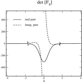
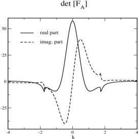
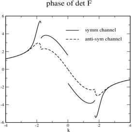
Figure 1: The left and middle panels show the Jost determinants in the symmetric and anti-symmetric channels for the potential, Eq. (15) with $v_{11}=4.0,\,v_{22}=1,\,v_{12}=0.5$ and $w=2.0$. The mass parameters are $m_{1}=1$ and $m_{2}=2$. The right panel shows their phases for the same set of parameters.

                   

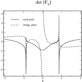
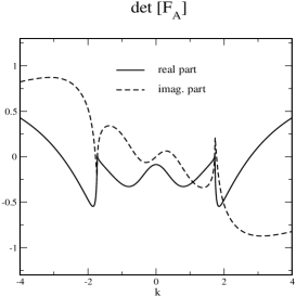
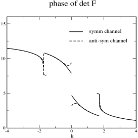
Figure 2: Same as figure 1 with $V_{0}\to-V_{0}$.

The real and imaginary parts of the Jost determinants are clearly even and odd functions of the single momentum variable $k$, respectively. Discontinuities or even singularities may occur at threshold $k^{2}=m_{2}^{2}-m_{1}^{2}$ and at $k=0$, which combine with jumps in the phases when bound states exist as required by Levinson’s theorem. For repulsive potentials, this theorem implies Barton:1984py $\lim_{k\to 0^{+}}\delta_{S}(k)=-\frac{\pi}{2}$. Hence the only phase without a jump is for a repulsive potential in the anti-symmetric channel. Yet, that phase still exhibits threshold cusps. For the attractive potential we also observe rapid changes slightly below threshold. They reflect Feshbach resonances, also called bound states in the continuum Newton:1982qc . In total, the Jost determinants defined in Eq. (14) combined with Eq. (5) have exactly the expected features describing physical scattering for real $k$. We have checked these results for other values of $V_{0}$ and $w$ as well.

A particularly interesting case is that of a system with interactions only in the heavy particle channel. The phase shift is treated as a function of the lighter particle’s momentum and therefore must vanish inside the gap, or at least be a (piecewise constant) multiple of $\pi$. If it did not, the VPE would not be the simple sum of the two particles’ VPEs when the potential matrix is diagonal.

                   

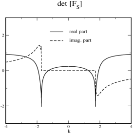
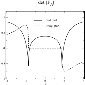
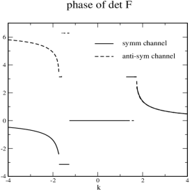
Figure 3: Real and imaginary parts and phases of the Jost determinants, Eq. (14) for $v_{11}=v_{12}=0$, $v_{22}=-2$ and $w=2$.

This property is verified in Figure 3. This result relies crucially on including the kinematic factors exactly as in Eq. (14). Also, the jumps by $\pi$ within the gap are significant for the VPE, as will be discussed in Appendix B.

For the parameters of Figure 3, a close inspection of the symmetric channel reveals that the phase shift jumps from $0$ to $\pi$ at $k=1.270$ and from $\pi$ to $\frac{\pi}{2}$ at threshold. These jumps hamper the continuous construction of phase shifts. In the anti-symmetric channel a jump occurs at $k=1.615$, while this phase shift is continuous at threshold. Even though the imaginary parts of the Jost determinants are zero within the gap, the jumps at $k=1.270$ and $k=1.615$ result from sign changes of the real parts as can also be observed from Figure 3. When the off-diagonal elements of $V_{0}$ are switched on, ${\sf Im}\,{\rm det}F\neq 0$ and ${\rm det}F$ has no zeros along the real axis. At the same time, the bound states from the uncoupled situation turn into (sharp) Feshbach resonances corresponding to zeros in the lower half of the complex momentum plane. We will comment further on this point at the end of Appendix A.

This discussion also reveals another interesting property of the phase shift related to Levinson’s theorem. For single-channel scattering, this theorem states that the phase shift at zero momentum is $\pi$ times the number of bound states in the anti-symmetric channel, However, for the symmetric channel, the ratio between the phase shift at zero momentum and $\pi$ equals the number of bound states minus $\frac{1}{2}$ Barton:1984py . For a two-channel problem one might therefore expect the phase shift at zero momentum to be $\pi$ times the number of bound states minus 1. The right panels of Figures 1, 2 and 3 show that this is not the case. Rather, the discontinuities that result from Levinson’s theorem appear at the respective thresholds. This is evident for the uncoupled system, and persists when the off-diagonal elements of the potential matrix are switched on, though the jump is slightly smoothed out in that case.

To identify genuine bound states as well as Feshbach resonances independently from the Jost function calculation we diagonalize the Hamiltonian

$$H=-\mbox{{\sf 1}\mbox{}\rule{0.39993pt}{6.6736pt}\mbox{\hskip 1.00006pt}}\frac{d^{2}}{dx^{2}}+\begin{pmatrix}m_{1}^{2}&0\cr 0&m_{2}^{2}\end{pmatrix}+V(x)$$ (16)

associated with the field Equation (3) in a discretized basis. The $2N$ basis wave-functions in the symmetric channel are

$$\Phi^{(0)}_{n}(x)=\frac{1}{\sqrt{2L}}\begin{pmatrix}{\rm cos}(p_{n}x)\cr 0\end{pmatrix}\qquad{\rm and}\qquad\Phi^{(0)}_{n+N}(x)=\frac{1}{\sqrt{2L}}\begin{pmatrix}0\cr{\rm cos}(p_{n}x)\end{pmatrix}\,,$$ (17)

with $x\in[0,L]$, which is sufficient since the potential is symmetric. The discretized momenta $p_{n}$ are determined such that $\Phi^{(0)}(L)=0$. Replacing ${\rm cos}(px)\,\rightarrow\,{\rm sin}(qx)$ gives the basis wave-functions in the anti-symmetric channel, where we must also redefine the discretized momenta $p_{n}\to q_{n}$ in order to maintain $\Phi^{(0)}(L)=0$. In general the eigenvalues $\omega^{2}$ of $H$ depend on $L$. However, this is not the case for bound states when $L$ is sufficiently large, because their wave-functions vanish at spatial infinity. Similarly the Feshbach resonances are associated with those eigenvalues in the continuum that do not vary when $L$ is altered. For the parameters of Figure 2 we observe bound state eigenvalues at $\omega^{2}=-2.128$ and $\omega^{2}=0.603$ in the symmetric channel. They correspond to $\kappa=1.768$ and $\kappa=0.630$. This agrees with Levinson’s theorem, since the phase shift at zero momentum equals $\frac{3\pi}{2}$. In the anti-symmetric channel only a single eigenvalue at $\omega^{2}=-0.513$ with $\kappa=1.230$ occurs. Accordingly, the phase shift equals $\pi$ at zero momentum. In the symmetric channel, a Feshbach resonance appears with the eigenvalue $\omega^{2}=3.435$, i.e. $k=1.560$, causing the corresponding phase shift to be $\frac{\pi}{2}$ at threshold. The Feshbach resonance in the anti-symmetric channel is just below threshold. It has the eigenvalue $\omega^{2}=3.968$, i.e. $k=1.723$ and the phase shift jumps by $\pi$ at threshold. Increasing the potential strength slowly moves this eigenvalue deeper into the gap, e.g. $v_{22}=1.2$ yields the eigenvalue $\omega^{2}=3.922$, while the resonance disappears for $v_{22}=0.6$ and the phase shift becomes continuous at threshold, though the typical cusps remains. We conclude that the Jost determinant as defined in Eq. (14) together with the definition of the dependent momentum variable, Eq. (5), possess all required properties for real momenta.

Finally, it is interesting to compute the $\omega^{2}$ eigenvalues for the parameters of Figure 3, i.e. the case when the lighter particle does not interact. We have observed bound states below $m_{2}^{2}$ at $\omega^{2}=2.613$ and $\omega^{2}=3.608$ in the symmetric and anti-symmetric channels, respectively. These bound state energies correspond to momenta $k_{2}$ on the positive imaginary axis that relate to real $k$ when $\omega^{2}>m_{1}^{2}$. Hence at these values of $k$ the phase shifts jump by $\pi$, as shown in the right panel of Figure 3.

When the coupling to the lighter particle is switched on again, these bound states turn into Feshbach resonances because the heavier particle may decay into the lighter one. Then a key additional property of the Jost determinant is that its only zeros (simple zeros in single channel scattering) are at purely imaginary bound state momenta $k=k_{1}={\rm i}\kappa_{i}$. Therefore we consider the Jost determinant for real $t$ defined via $k={\rm i}t$, so that the differential equation, Eq. (3), is purely real (the ${\rm i}\epsilon$ prescription can be omitted for $t>0$) and so is the Jost determinant. In Figure 4 we show the corresponding numerical results.

                 

Figure 4: The real Jost determinant for $k={\rm i}t$. The left and right panels corresponds to the parameters of Figures 1 and 2, respectively. Note the different scales for the vertical axes.

The positions of the zeros of ${\rm det}F$ clearly agree with the above listed values for $\kappa_{i}$. In the symmetric channel the determinant diverges as $t\to 0$ because of $D^{-1}$ in Eq. (14). This is actually the origin for the $\frac{\pi}{2}$ in Levinson’s theorem. This divergence is not a serious problem here because the VPE is only sensitive to $t\geq m_{1}$. At large $t$ the determinant approaches unity, though this asymptotic value is assumed only slowly. Without any bound states the Jost determinant is positive along the positive imaginary axis.

In appendix A we present further numerical analysis of the Jost determinant using Cauchy integrals.

IV Skewed Parity

So far we have studied the case of a completely symmetric potential matrix. For the model of Ref. Bazeia:1995en , we will consider potential matrices symmetric under skewed parity,

$$V(-x)=\begin{pmatrix}1&0\cr 0&-1\end{pmatrix}V(x)\begin{pmatrix}1&0\cr 0&-1\end{pmatrix}\,.$$ (18)

That is, diagonal and off–diagonal elements of the potential matrix are even and odd functions of the coordinate, respectively. Similar to the Dirac theory we introduce a parity operator

$$\hat{P}\Phi(x)=\hat{P}\begin{pmatrix}\phi_{1}(x)\cr\phi_{2}(x)\end{pmatrix}=\begin{pmatrix}\phi_{1}(-x)\cr-\phi_{2}(-x)\end{pmatrix}$$ (19)

that has eigenvalues $\lambda_{p}=\pm 1$. It is then convenient to define the projectors

$$P_{+}=\begin{pmatrix}1&0\cr 0&0\end{pmatrix}\qquad{\rm and}\qquad P_{-}=\begin{pmatrix}0&0\cr 0&1\end{pmatrix}\,,$$ (20)

so that $\phi_{1}(x)=P_{+}\Phi(x)$ and $\phi_{2}(x)=P_{-}\Phi(x)$. In this notation the channel with $\lambda_{p}=1$ has

$$P_{+}\partial_{x}\Phi_{+}(0)=0\qquad{\rm and}\qquad P_{-}\Phi_{+}(0)=0\,,$$

while the $\lambda_{p}=-1$ channel has

$$P_{-}\partial_{x}\Phi_{-}(0)=0\qquad{\rm and}\qquad P_{+}\Phi_{-}(0)=0\,.$$

The Jost matrices for the two parity channels can also be obtained from the solution of Eq. (10). Suitable projection yields

$$F_{\pm}(k)=\left[P_{\pm}F_{S}(k)D_{\mp}(k)+P_{\mp}F_{A}(k)D_{\pm}^{-1}(k)\right]\,.$$ (21)

The factor matrices

$$D_{+}(k)=\begin{pmatrix}{\rm i}k&0\cr 0&1\end{pmatrix}\qquad{\rm and}\qquad D_{-}(k)=\begin{pmatrix}1&0\cr 0&{\rm i}k_{2}\end{pmatrix}\,,$$

with $k_{2}$ being again related to $k$ via Eq. (5), ensure that $\lim_{|k|\to\infty}F_{\pm}(k)=\mbox{{\sf 1}\mbox{}\rule{0.39993pt}{6.6736pt}\mbox{\hskip 1.00006pt}}$. Note that any right multiplication of $F(k,x)$ in Eq. (9) by a constant matrix is a solution to the field Equation (10) and translates into a right multiplication of $Z(k,x)$ when this constant matrix is diagonal.

In the positive parity channel the bound state energies, and eventually the position of the Feshbach resonances, are obtained by diagonalizing the Hamiltonian, Eq. (16) with respect to the $2N$ basis states

$$\Phi^{(0)}_{n}(x)=\frac{1}{\sqrt{2L}}\begin{pmatrix}{\rm cos}(p_{n}x)\cr 0\end{pmatrix}\qquad{\rm and}\qquad\Phi^{(0)}_{n+N}(x)=\frac{1}{\sqrt{2L}}\begin{pmatrix}0\cr{\rm sin}(q_{n}x)\end{pmatrix}\,.$$ (22)

Again the discretized momenta $p_{n}$ and $q_{n}$ are obtained from $\Phi^{(0)}(L)=0$. The basis states in the negative parity channel are constructed by swapping upper and lower components.

Using the trial potential matrix

$$V(x)=V_{1}(x)\,{\rm exp}\left(-\frac{x^{2}}{w^{2}}\right)\qquad{\rm with}\qquad V_{1}(x)=\begin{pmatrix}v_{11}&v_{12}\,x\cr v_{12}\,x&v_{22}\end{pmatrix}$$

we have repeated the numerical experiments from Section III and appendix A and established that the determinants defined by the matrices of Eq. (21) have the standard Jost function properties discussed in Section II.

V Formulation of Vacuum Polarization Energy

Formally the VPE is the sum of the shifts of zero-point energies due to the interaction with the potential $V(x)$. It can be decomposed as Graham:1999pp

$$E_{\rm vac}=\frac{1}{2}\sum_{\omega_{i}^{2}\leq m_{1}^{2}}\left[\omega_{i}-m_{1}\right]+\int_{0}^{\infty}\frac{dk}{2\pi}\,\left[\omega(k)-m_{1}\right]\frac{d}{dk}\sum_{s}\delta_{s}(k)\Big{|}_{\rm ren.}\,.$$ (23)

where the discrete sum is over the bound state energies (excluding Feshbach resonances) and $k$ labels the continuum scattering states with energy $\omega(k)$ such that $k=0$ denotes the scattering threshold. According to the Krein formula Faulkner:1977aa the derivative of the total phase shift,

$$\delta_{s}(k)=\frac{1}{2{\rm i}}{\rm ln}\,{\rm det}S_{s}(k)=\frac{1}{2{\rm i}}\left[{\rm ln}\,{\rm det}F_{s}(-k)-{\rm ln}\,{\rm det}F_{s}(k)\right]$$ (24)

in channel $s$ gives the change in the density of scattering states. These channels can either be the symmetric and anti-symmetric channels discussed in Sections II and III, or the parity modes from the previous Section. We note that Eq. (23) can also be derived from the energy-momentum tensor in field theory Graham:2002xq . Finally the subscript “ren.” indicates that, as it stands, the integral diverges and requires regularization and renormalization. Working in one space dimension, the Born approximation

$$\delta^{(1)}(k)=-\frac{1}{k}\int_{0}^{\infty}dx\,V_{11}(x)-\frac{1}{\sqrt{k^{2}-m_{2}^{2}+m_{1}^{2}}}\int_{0}^{\infty}dx\,V_{22}(x)$$ (25)

is typically subtracted under the integral to impose the no-tadpole renormalization condition, which removes all terms linear in $V(x)$ from the VPE. While the pole at $k=0$ is canceled by the factor $\omega(k)-m_{1}\,\rightarrow\,{\textstyle\frac{k^{2}}{2m_{1}}}$ as $k\to 0$, the singularity at threshold $k=\sqrt{m_{2}^{2}-m_{1}^{2}}$ precludes a direct application of this prescription when different mass parameters are involved. Since

$$\Delta^{(1)}(k)=-\frac{1}{k}\int_{0}^{\infty}dx\,V_{11}(x)-\frac{1}{k}\int_{0}^{\infty}dx\,V_{22}(x)$$ (26)

has the same large $k$ behavior as $\delta^{(1)}(k)$, it serves well as a helper function such that

$$\widetilde{E}_{\rm vac}=\frac{1}{2}\sum_{\omega_{i}^{2}\leq m_{1}^{2}}\left[\omega_{i}-m_{1}\right]+\int_{0}^{\infty}\frac{dk}{2\pi}\,\left[\omega(k)-m_{1}\right]\frac{d}{dk}\left[\left(\sum_{s}\delta_{s}(k)\right)-\Delta^{(1)}(k)\right]$$ (27)

is finite. In contrast to $\delta^{(1)}(k)$ which has a square root branch cut, $\Delta^{(1)}(k)$ is analytic up the pole at $k=0$ which is removed by the factor $\omega(k)-m_{1}$.

Although $\widetilde{E}_{\rm vac}$ is finite, it does not obey the no-tadpole renormalization condition. By analytic continuation we will next obtain an integral expression for the VPE that allows us to replace $\Delta^{(1)}$ by $\delta^{(1)}$ and also avoids integrating over the various cusps (or even jumps) of the phase shift within the gap. In a first step we use Eq. (24), replace $\delta_{s}(k)$ by the odd function ${\rm ln}\,{\rm det}F_{s}(k)$ and express the VPE as a single integral along the whole real axis,

$$\widetilde{E}_{\rm vac}=\frac{1}{2}\sum_{\omega_{i}^{2}\leq m_{1}^{2}}\left[\omega_{i}-m_{1}\right]-\int_{-\infty}^{\infty}\frac{dk}{4\pi{\rm i}}\,\left[\omega(k)-m_{1}\right]\frac{d}{dk}\left[\left(\sum_{s}{\rm ln}\,{\rm det}F_{s}(k)\right)-\Delta^{(1)}(k)\right]\,.$$

As numerically verified in Appendix A, $\frac{d}{dk}{\rm ln}\,{\rm det}F_{s}(k)$ has first order poles with unit residue exactly at those imaginary momenta that represent the bound state energies $\omega_{i}$. When closing the contour in the upper half plane, these poles compensate the explicit contributions from the bound states, i.e. the first term in the above equation. The only contribution then comes from enclosing the branch cut along the imaginary axis ($t\in\mathbb{R}$)

$$\sqrt{m_{1}^{2}+({\rm i}t+\epsilon)^{2}}-\sqrt{m_{1}^{2}+({\rm i}t-\epsilon)^{2}}=2{\rm i}\sqrt{t^{2}-m_{1}^{2}}\qquad{\rm for}\quad t\geq m_{1}\,,$$

yielding

$$\widetilde{E}_{\rm vac}=-\int_{m_{1}}^{\infty}\frac{dt}{2\pi}\,\sqrt{t^{2}-m_{1}^{2}}\,\frac{d}{dt}\left[\left(\sum_{s}{\rm ln}\,{\rm det}F_{s}({\rm i}t)\right)-\Delta^{(1)}({\rm i}t)\right]\,.$$

Finally we integrate by parts and obtain

$$\widetilde{E}_{\rm vac}=\int_{m_{1}}^{\infty}\frac{dt}{2\pi}\frac{t}{\sqrt{t^{2}-m_{1}^{2}}}\,\left[\nu(t)-\Delta^{(1)}(t)\right]$$

where

$$\nu(t)\equiv{\rm ln}\,{\rm det}\left[F_{+}({\rm i}t)\,F_{-}({\rm i}t)\right]$$ (28)

denotes the summed exponentials of the Jost determinants. Without difficulty we can now restore the original no-tadpole scheme,

$$E_{\rm vac}\equiv\int_{m_{1}}^{\infty}\frac{dt}{2\pi}\frac{t}{\sqrt{t^{2}-m_{1}^{2}}}\,\left[\nu(t)-\nu^{(1)}(t)\right]\,,$$ (29)

where we have replaced $\Delta^{(1)}({\rm i}t)$ with

$$\nu^{(1)}(t)=\int_{0}^{\infty}dx\,\left[\frac{V_{11}(x)}{t}+\frac{V_{22}(x)}{\sqrt{t^{2}+m_{2}^{2}-m_{1}^{2}}}\right]\,.$$ (30)

It is obvious that this subtraction fully removes the $\mathcal{O}(V)$ contribution to the VPE. Up to a factor of ${\rm i}$ it is the continuation of the Born approximation, Eq. (25), to the imaginary axis. Formally Eqs. (29)-(30) are standard Graham:2009zz , except for the second denominator in the Born approximation. It clearly reflects the infra-red singularity at $k^{2}=m_{2}^{2}-m_{1}^{2}$ above. Fortunately, that is not an issue when we integrate along the imaginary axis.

Without off-diagonal interactions $\nu$ and $\nu^{(1)}$ are the sums of the Jost functions for the two particles with the imaginary momentum variables $t$ and $\sqrt{t^{2}+m_{2}^{2}-m_{1}^{2}}$, respectively. Thus it is obvious that Eq. (29) is just the sum of the individual contributions, as it should be. This is also the case for the real momentum formulation, Eq. (27). However, the additivity is less obvious on the real axis because it requires careful consideration of the phase shift within the gap, as we will discuss in Appendix B.

VI Bazeia Model

The Bazeia model Bazeia:1995en generalizes the $\phi^{4}$ kink model in one space and one time dimensions by introducing a second scalar field $\chi$. Since the model admits various soliton solutions that are classically degenerate it is a prime candidate to apply the above developed method to compute the VPE and investigate whether this degeneracy is lifted by quantum corrections. In this Section, we adopt the notation for the fields from the original paper Bazeia:1995en , $(\Phi_{1},\Phi_{2})\,\longrightarrow\,(\phi,\chi)$. The mass terms are included in the field potential, $U(\phi,\chi)$, in contrast to Eq. (2).

After appropriate rescaling of the fields and the coordinates the Lagrangian

$$\mathcal{L}=\frac{1}{2}\left[\partial_{\mu}\phi\partial^{\mu}\phi+\partial_{\mu}\chi\partial^{\mu}\chi\right]-U(\phi,\chi)\,,\qquad{\rm with}\qquad U(\phi,\chi)=\frac{1}{2}\left[\phi^{2}-1+\frac{\mu}{2}\chi^{2}\right]^{2}+\frac{\mu^{2}}{2}\phi^{2}\chi^{2}$$ (31)

is characterized by the single parameter $\mu$. The vacuum configuration is $\phi_{\rm vac}=\pm 1$ and $\chi_{\rm vac}=0$ so that $m_{\chi}=\mu$ and $m_{\phi}=2$. Subtracting the mass terms from $\partial^{2}U$ yields the fluctuation potential matrix

$$V\equiv\partial^{2}U-\begin{pmatrix}\mu^{2}&0\\[5.69054pt] 0&4\end{pmatrix}=\begin{pmatrix}\mu(1+\mu)\left(\phi^{2}-1\right)+\frac{3}{2}\mu^{2}\chi^{2}&2\mu(1+\mu)\chi\phi\\[5.69054pt] 2\mu(1+\mu)\chi\phi&6\phi^{2}-6+\mu(\mu+1)\chi^{2}\end{pmatrix}\,.$$ (32)

Later we will be interested solely in the case $\mu\leq 2$. Then $\chi$ is the lighter particle and hence plays the role of $\Phi_{1}$.

There is always the pure kink soliton

$$\phi^{(1)}={\rm tanh}(x)\qquad{\rm and}\qquad\chi^{(1)}=0\,.$$ (33)

In addition, for $\mu\leq 1$ a second solution is

$$\phi^{(2)}={\rm tanh}(\mu x)\qquad{\rm and}\qquad\chi^{(2)}=\frac{\sqrt{2\left(1/\mu-1\right)}}{{\rm cosh}(\mu x)}\,.$$ (34)

The construction of these solitons is described in Ref. Bazeia:1995en . For $\mu=1$ the two solutions are identical. They are actually degenerate in classical mass, $E_{\rm cl}=\frac{4}{3}$ since the model is defined such that $E_{\rm cl}$ can be uniquely determined from the asymptotic values of the fields. The specific cases of the fluctuation potential Eq. (32) for the two soliton solutions (33) and (34) are

$$V^{(1)} =\frac{-1}{{\rm cosh}^{2}(x)}\begin{pmatrix}\mu(1+\mu)&0\\[5.69054pt] 0&6\end{pmatrix}\,,$$ (35)

$$V^{(2)} =\frac{1}{{\rm cosh}^{2}(x)}\begin{pmatrix}2\mu-4\mu^{2}\qquad&2(1+\mu)\sqrt{2\mu(1-\mu)}\,{\rm sinh}(\mu x)\\[5.69054pt] 2(1+\mu)\sqrt{2\mu(1-\mu)}\,{\rm sinh}(\mu x)&-4-2\mu^{2}\end{pmatrix}\,.$$ (36)

Since $\phi$ is the heavier particle, the translational zero mode wave-function is odd in the upper component and even in the lower one. Hence this zero mode lives in the negative parity channel. However, we also observe a zero mode in the positive parity channel. This second zero mode can be used to construct a family of soliton solutions parameterized by $|\chi(0)|\leq\sqrt{{\textstyle\frac{2}{\mu}}}$. This family has already been found in the context of supersymmetric domain wall models Shifman:1997wg . Except for the particular cases $\mu={\textstyle\frac{1}{2}}$ and $\mu=2$, which lead to the solitons discussed in Eqs. (37) and  (38) below, these solitons can only be formulated numerically; we will provide a detailed discussion of their VPEs elsewhere HNM .

For $\mu=1$ the particles decouple and the heavier one is subject to the potential $v_{22}(x)=-6/{\rm cosh}^{2}(x)$ which is known to have a zero mode and a bound state, the so-called shape mode, at $\omega^{2}=3$ (for $m_{2}=2$) Ra82 . This corresponds to the imaginary dependent momentum $k_{2}={\rm i}$ and to the real independent momentum $k=\sqrt{2}$ since $m_{1}=1$ and $m_{2}=2$. This is a soliton example of a Feshbach resonance. Hence this state is not explicitly counted in the discrete sum in Eq. (23). Indeed for this real momentum the Jost determinant of the positive parity channel is zero and the phase shift jumps by $\pi$.

$\mu$	2.0	1.5	1.0	0.9	0.8	0.7	0.6	0.5	0.4	0.3	0.2
Eq. (33)	-1.333	-1.151	-0.985	-0.953	-0.922	-0.891	-0.860	-0.830	-0.799	-0.768	-0.737
Eq. (34)	—	—	-0.985	-0.969	-0.960	-0.961	-0.976	-1.011	-1.085	-1.228	-1.540

Table 1: Vacuum polarization energies for the Bazeia model as computed from Eq. (29).

In Table 1 we list the numerical results for the VPEs of the two soliton solutions. For the simple diagonal case, Eq. (35), we agree with the heat kernel results: the top line in Table 1 is obtained by adding the $\sigma=2$ and $\sigma=\mu$ entries of Table 4 in Ref. AlonsoIzquierdo:2012tw . To our knowledge, there are no previous studies on the off-diagonal case, Eq. (36), in the literature.

Note that the $\mu=2$ entry corresponds to $2\times\left(\frac{1}{2\sqrt{3}}-\frac{3}{\pi}\right)\sim-1.3326$, i.e. twice the $\phi^{4}$–kink vacuum polarization energy for quantum fluctuations with mass $m_{2}=2$. The case $\mu=1$ is even more interesting not only because the two solitons are identical, but also because it is an application of our general method to the particular case of zero off-diagonal potential matrix elements, since $\chi\equiv 0$, but with an actual gap present (see also Appendix B). While $v_{11}(x)=-2/{\rm cosh}^{2}(x)$ is the potential for fluctuations off the sine-Gordon soliton with mass $m_{1}=1$, $v_{22}(x)=-6/{\rm cosh}^{2}(x)$ is the potential for fluctuations off the $\phi^{4}$ kink with mass $m_{2}=2$. Indeed our numerical result equals the sum of these well-established VPEs Ra82 ; Graham:2009zz , $\left(\frac{1}{2\sqrt{3}}-\frac{3}{\pi}\right)-\frac{1}{\pi}\sim-0.9846$, providing verification of the threshold treatment in particular, since the shape mode of the $\phi^{4}$ part has disappeared as a manifest bound state. The coupled channel formalism treats the two uncoupled particles in such a way that the shape mode of the heavier particle is no longer a zero of the Jost determinant on the imaginary $k$-axis. As discussed earlier, this is a kinematical feature induced by relating the momenta between the heavier and lighter particles.

As mentioned, the two solitons are classically degenerate. Obviously including one loop quantum corrections favors the second solution. The present conventions yield $E_{\rm cl}=\frac{4}{3}$ suggesting that for small enough $\mu$ the soliton, Eq. (34) would unavoidably be destabilized by quantum corrections. These convenient conventions included scaling the fields by $\frac{1}{\sqrt{\lambda}}$, where $\lambda$ is the fourth order coupling constant when the coefficient of the quadratic order does not contain $\lambda$. However, in quantum field theory the scale of the field cannot be chosen freely; rather, it is dictated by the equal-time commutation relations. Though this is irrelevant when comparing various VPEs in a given model, it must be taken into consideration when combining classical and quantum contributions. When (re)introducing physical parameters, $E_{\rm cl}$ scales like $\frac{1}{\lambda}$, but $E_{\rm vac}$ does not depend on $\lambda$ Ra82 ; Graham:2009zz . It is then clear that the occurrence of instability depends on the interaction strength.

Also note that for $\mu=2$ the VPE is twice that of the $\phi^{4}$ model kink even though it is the same soliton configuration. This is due to the addition of $\chi$ type quantum fluctuations. The case $\mu=2$ is also interesting because there is an additional soliton solution

$$\phi^{(3)}=\frac{{\rm sinh}(2x)}{b+{\rm cosh}(2x)}\qquad{\rm and}\qquad\chi^{(3)}=\frac{\sqrt{b^{2}-1}}{b+{\rm cosh}(2x)}\,$$ (37)

with an arbitrary parameter $b>1$. For $b=1$ this becomes the standard kink configuration. The classical energy is the same for all allowed values of $b$. As already observed in the heat kernel calculation of Ref. AlonsoIzquierdo:2003gh , we find that also the VPE does not vary with $b$. Actually the Jost determinant itself turns out not to depend on $b$. The reason is simple: for $\mu=2$ the transformation

$$\phi=\frac{\eta_{1}+\eta_{2}}{2}\qquad{\rm and}\qquad\chi=\frac{\eta_{1}-\eta_{2}}{2}$$

decouples the potential, Eq. (31) into two $\phi^{4}$ models for $\eta_{1}$ and $\eta_{2}$ AlonsoIzquierdo:2003gh . The configuration of Eq. (37) corresponds to individual kinks for $\eta_{i}$ separated by ${\rm arcosh}(b)$. The solution $\eta_{1}={\rm tanh}(x)$ and $\eta_{2}(x)=1$ translates into $\phi(x)=\left[{\rm tanh}(x)+1\right]/2$ and $\chi(x)=\left[{\rm tanh}(x)-1\right]/2$. This case is interesting because it induces the symmetric potential matrix

$$V(x)=\frac{-3}{{\rm cosh}^{2}(x)}\begin{pmatrix}1&1\cr 1&1\end{pmatrix}\,,$$

which has a zero eigenvalue. The vacuum polarization energy must then be computed from $F_{S}$ and $F_{A}$ defined in Eq. (14). It is reassuring that our numerical simulation yields $E_{\rm vac}=-0.6625$, consistent with the known VPE of a single kink. But then, the case $\mu=2$ is not a stringent litmus test for our approach because it does not exhibit a mass gap.

As mentioned, for $\mu=\frac{1}{2}$ yet another soliton solution is known analytically Shifman:1997wg

$$\phi^{(4)}=\frac{(1-a^{2}){\rm sinh}(x)}{a^{2}+(1-a^{2}){\rm cosh}(x)}\qquad{\rm and}\qquad\chi^{(4)}=\sqrt{\frac{2}{\mu}}\,\frac{a}{\sqrt{a^{2}+(1-a^{2}){\rm cosh}(x)}}$$ (38)

with $|a|<1$. The case $a=0$ reproduces the pure kink soliton. Though the case $|a|=1$ solves the field equations, it is not a soliton Bazeia:1995en because it is not localized. Consequently, the corresponding potential matrix, Eq. (32) does not vanish at spatial infinity. Comparing the numerical results Tables 1 and 2, we see that the limiting case $a\to 1$ has an even lower VPE than the second soliton, Eq. (34), for $\mu=\frac{1}{2}$.

$a$	0.0	0.2	0.4	0.6	0.8
Eq. (38)	-0.830	-0.841	-0.878	-0.949	-1.089

Table 2: Vacuum polarization energies for the soliton of Eq. (38) in the Bazeia model with $\mu=\frac{1}{2}$ as computed from Eq. (29).

VII Conclusion

We have generalized the spectral methods for computing the vacuum polarization energy (VPE) of static solitons to models containing coupled fields with different mass parameters. This result is non-trivial endeavor because the spectral methods rely on the analytic properties of scattering data, most prominently the Jost function/determinant $F$, but different masses induce a non-analytic relation between the momenta that describe the asymptotic behavior of the fields. Taking $k$ to be the momentum associated with the smaller mass, the essential ingredient is to establish a relation, Eq. (5), between the two momenta that fulfills $F^{\ast}(k)=F(-k)$ for all real $k$ and that preserves the analytic properties of $F(k)$ in the upper half complex momentum plane, ${\sf Im}(k)\geq 0$. We have checked this relation by numerically verifying those properties for different potentials. The formulation of the VPE is then similar to the case without a mass gap. However, it is indispensable to consider momenta off the real axis because the no-tadpole renormalization condition would otherwise induce a singularity for models in one space dimension. Once the generalized spectral method is established, the computation of the VPE is numerically straightforward and does not require any further approximation or expansion. We have then applied this formalism to a soliton model with two real scalar fields to (i) verify that the approach is consistent and (ii) to show that the VPE, i.e. the quantum correction to the soliton mass, lifts the classical degeneracy.

There are many other soliton models in one space dimension to which the formalism can be applied. For example, the solitons constructed in Refs. Sarkar:1976vr ; Montonen:1976yk have different classical masses and it would be interesting to see whether the respective VPEs obey the same inequality.

Obviously the formalism is not constrained to one space dimension but can be applied in higher dimensions with cylindrical or spherical symmetry. A prime candidate for future investigation is the VPE of the ’t Hooft-Polyakov monopole tHooft:1974kcl ; Polyakov:1974ek .

Appendix A Cauchy integrals of the Jost determinant

To further analyze the analytic structure of the Jost determinant we we take the potential model from Eq. (15) and consider contours parameterized by a complex center, $k_{0}$ and a radius $R$:

$$\mathcal{C}(\alpha)\,:\,\,k=k_{0}+R\,{\rm e}^{{\rm i}\varphi}\qquad{\rm with}\qquad\varphi=0\ldots\alpha\,,$$ (39)

which describe full circles when $\alpha=2\pi$. For these contours we numerically compute the line integrals

$$I_{\rm det}(\alpha) =\int_{\mathcal{C}(\alpha)}\,dk\,{\rm det}F(k)\qquad\qquad{\rm and}$$ (40)

$$I_{\rm log}(\alpha) =\int_{\mathcal{C}(\alpha)}\,dk\,\frac{d}{dk}{\rm ln}\,{\rm det}F=\int_{\mathcal{C}(\alpha)}\,dk\,\frac{1}{{\rm det}F(k)}\frac{d}{dk}{\rm det}F(k)\,.$$ (41)

In Figure 5 we show typical results for these contour integrals.

                   

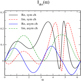
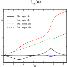
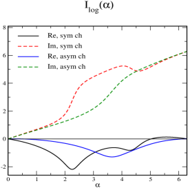
Figure 5: (Color online)Contour integrals $I_{\rm det}(\alpha)$ and $I_{\rm log}(\alpha)$ defined in Eq. (41) for the model parameters of Figure 2. The parameters for the line integral, Eq. (39) are $k_{0}=1.2{\rm i}$ and $R=1$ (left and middle panel); $k_{0}=0.3+1.4{\rm i}$ and $R=0.6$ (right panel).

For any considered contour (including paths composed of piece-wise linear sections) in the upper half complex plane we found results for $I_{\rm det}(\alpha)$ as in the left panel. Though there are some oscillations as function of $\alpha$, the line integrals vanish when the circles are completed. When the contour enters the lower half plane, the integrals cannot be controlled numerically. Also the results from the middle and left panels are as expected for a well-behaved Jost determinant. The integral $I_{\rm log}(2\pi)$ counts the enclosed zeros in multiples of $2\pi{\rm i}$. The contour of the middle figure encloses all bound states identified in Section III and thus we find $4\pi{\rm i}$ and $2\pi{\rm i}$ for the symmetric and anti-symmetric channels, respectively. The higher bound state in the symmetric channel is not enclosed by the contour of the right panel. Hence in that case we obtain $2\pi{\rm i}$ for both channels.

The zeros in the lower half complex momentum plane that correspond to Feshbach resonances cannot be identified by computing $I_{\rm log}$ because the Jost determinant is not expected to be an analytic function in that regime. However, we can test whether the zeros of Figure 3 unexpectedly moved to the upper half plane. To this end we consider a contour defined by the triangle $k=1.0+0.0001\,{\rm i}\,\rightarrow\,2.0+0.0001\,{\rm i}\,\rightarrow\,1.5+{\rm i}\,\rightarrow\,1.0+0.0001\,{\rm i}$ for different values of the off-diagonal elements of $V_{0}$, $v_{12}=0.01$ and $v_{12}=0.2$. In the vicinity of the Feshbach resonances and the threshold the numerical integration requires tiny step sizes. In the end the numerical results for $I_{\rm log}$ are indeed compatible with zero.

Appendix B VPE for decoupled particles

In this appendix we will show that $\widetilde{E}_{\rm vac}$, Eq. (27) is additive when the two particles decouple. Since Eq. (27) is constructed in terms of the lighter particle’s momentum, it suffices to verify that

$$\widetilde{E}_{\rm vac}=\frac{1}{2}\sum_{\omega_{i}^{2}\leq m_{2}^{2}}\left[\omega_{i}-m_{2}\right]+\int_{0}^{\infty}\frac{dq}{2\pi}\,\left[\sqrt{q^{2}+m_{2}^{2}}-m_{2}\right]\frac{d}{dq}\overline{\delta}(q)$$ (42)

follows from Eq. (27) when $V(x)=\begin{pmatrix}0&0\cr 0&v(x)\end{pmatrix}$ where $\overline{\delta}(q)$ is the phase shift for the scattering problem

$$q^{2}\psi(x)=-\partial_{x}^{2}\psi(x)+v(x)\psi(x)\,,$$

with $\Delta^{(1)}(q)$, as defined in Eq. (26) with $V_{11}(x)=0$ and $V_{22}(x)=v(x)$, subtracted.

Let $n_{0}$ and $n_{1}$ be the number of bound states with $\omega_{i}^{2}\leq m_{1}^{2}$ and $m_{1}^{2}<\omega_{i}^{2}\leq m_{2}^{2}$, respectively. As discussed after Eq. (14) and in the context of Figure 3, each bound state with $\omega_{i}^{2}\leq m_{1}^{2}$ adds $\pi$ to the phase in $0\leq k\leq\overline{k}=\sqrt{m_{2}^{2}-m_{1}^{2}}$ and each bound state with $m_{1}^{2}<\omega_{i}^{2}\leq m_{2}^{2}$ adds $\pi$ from $k_{i}=\sqrt{\omega_{i}^{2}-m_{1}^{2}}$ to $\overline{k}$. Hence the phase shift that enters Eq. (27) is

$$\left(\sum_{s}\delta_{s}(k)\right)-\Delta^{(1)}(k)=n_{0}\pi\left[\theta(k)-\theta(k-\overline{k})\right]+\pi\sum_{m_{1}^{2}<\omega_{i}^{2}\leq m_{2}^{2}}\left[\theta(k-k_{i})-\theta(k-\overline{k})\right]+\theta(k-\overline{k})\,\overline{\delta}\left(\sqrt{k^{2}-\overline{k}^{2}}\right)\,,$$ (43)

where $\theta(k)$ is the Heaviside step function. The derivative with respect to the momentum $k$ produces various Dirac-$\delta$ functions that yield discrete contributions in Eq. (27). Noting that $\omega(0)=m_{1}$ and $\omega(\overline{k})=m_{2}$ we find

$$\widetilde{E}_{\rm vac} =\frac{1}{2}\sum_{\omega_{i}^{2}\leq m_{1}^{2}}\left(\omega_{i}-m_{1}\right)-\frac{n_{0}}{2}\left(m_{2}-m_{1}\right)+\frac{1}{2}\sum_{m_{1}^{2}<\omega_{i}^{2}\leq m_{2}^{2}}\left(\omega_{i}-m_{1}\right)-\frac{n_{1}}{2}\left(m_{2}-m_{1}\right)$$ (44)

$$\hskip 28.45274pt+\frac{1}{2\pi}\left(m_{2}-m_{1}\right)\overline{\delta}(0)+\int_{\overline{k}}^{\infty}\frac{dk}{2\pi}\,\left[\sqrt{k^{2}+m_{1}^{2}}-m_{1}\right]\frac{d}{dk}\overline{\delta}\left(\sqrt{k^{2}-\overline{k}^{2}}\right)$$ (45)

$$=\frac{1}{2}\sum_{\omega_{i}^{2}\leq m_{1}^{2}}\left(\omega_{i}-m_{2}\right)+\frac{1}{2}\sum_{m_{1}^{2}<\omega_{i}^{2}\leq m_{2}^{2}}\left(\omega_{i}-m_{2}\right)+\int_{\overline{k}}^{\infty}\frac{dk}{2\pi}\,\left[\sqrt{k^{2}+m_{1}^{2}}-m_{2}\right]\frac{d}{dk}\overline{\delta}\left(\sqrt{k^{2}-\overline{k}^{2}}\right)\,.$$ (46)

Changing the integration variable to $q$ by $k=\sqrt{q^{2}+\overline{k}^{2}}$ then yields indeed Eq. (42).

Often the VPE is formulated via integrating Eq. (27) by parts Graham:2009zz

$$\widetilde{E}_{\rm vac}=\frac{1}{2}\sum_{\omega_{i}^{2}\leq m_{1}^{2}}\left(\omega_{i}-m_{1}\right)-\int_{0}^{\infty}\frac{dk}{2\pi}\,\frac{k}{\omega(k)}\,\left[\left(\sum_{s}\delta_{s}(k)\right)-\Delta^{(1)}(k)\right]$$ (47)

since this quantity is better accessible numerically. Substituting Eq. (43) yields

$$\widetilde{E}_{\rm vac} =\frac{1}{2}\sum_{\omega_{i}^{2}\leq m_{1}^{2}}\left(\omega_{i}-m_{1}\right)-\frac{n_{0}}{2}\omega(k)\Big{|}_{k=0}^{k=\overline{k}}-\frac{1}{2}\sum_{m_{1}^{2}<\omega_{i}^{2}\leq m_{2}^{2}}\omega(k)\Big{|}_{k=k_{i}}^{k=\overline{k}}-\int_{\overline{k}}^{\infty}\frac{dk}{2\pi}\,\frac{k}{\sqrt{k^{2}+m_{1}^{2}}}\,\overline{\delta}\left(\sqrt{k^{2}-\overline{k}^{2}}\right)$$ (48)

$$=\frac{1}{2}\sum_{\omega_{i}^{2}\leq m_{1}^{2}}\left(\omega_{i}-m_{2}\right)-\frac{1}{2}\sum_{m_{1}^{2}<\omega_{i}^{2}\leq m_{2}^{2}}\left(m_{2}-\omega_{i}\right)-\int_{0}^{\infty}\frac{dq}{2\pi}\,\frac{q}{\sqrt{q^{2}+m_{2}^{2}}}\,\overline{\delta}\left(q\right)\,,$$ (49)

which is VPE in the form of Eq. (47) for a single particle with mass $m_{2}$.

References

- (1) R. Rajaraman, Solitons and Instantons, North Holland, 1988.
- (2) E. Farhi, N. Graham, R. L. Jaffe, H. Weigel, Nucl. Phys. B 585 (2000) 443.
- (3) H. Weigel, M. Quandt, N. Graham, Phys. Rev. Lett. 106 (2011) 101601.
- (4) N. Graham, M. Quandt, H. Weigel, Lect. Notes Phys. 777 (2009) 1.
- (5) J. Schwinger, Phys. Rev. 94 (1954) 1362.
- (6) R. F. Dashen, B. Hasslacher, A. Neveu, Phys. Rev. D 10 (1974) 4130.
- (7) J. Baacke, Z. Phys. C 47 (1990) 263; Z. Phys. C 53 (1992) 402.
- (8) N. Graham, R. L. Jaffe, V. Khemani, M. Quandt, M. Scandurra, H. Weigel, Nucl. Phys. B 645 (2002) 49.
- (9) M. Bordag, J. Phys. A 28 (1995) 755; M. Bordag, K. Kirsten, Phys. Rev. D 53 (1996) 5753; M. Bordag, M. Hellmund, K. Kirsten, Phys. Rev. D 61 (2000) 085008
- (10) E. Elizalde, Lect. Notes Phys. Monogr. 35 (1995) 1; K. Kirsten, AIP Conf. Proc. 484, 106 (1999).
- (11) A. Alonso-Izquierdo, J. Mateos Guilarte, Annals Phys. 327 (2012) 2251.
- (12) A. Alonso-Izquierdo, W. Garcia Fuertes, M. A. Gonzalez Leon, J. Mateos Guilarte, Nucl. Phys. B 681 (2004) 163.
- (13) H. Gies, K. Langfeld, L. Moyaerts, JHEP 0306 (2003) 018.
- (14) I. J. R. Aitchison, C. M. Fraser, Phys. Rev. D 31 (1985) 2605; G. V. Dunne, Phys. Lett. B 467 (1999) 238.
- (15) I. M. Gelfand, A. M. Yaglom, J. Math. Phys. 1 (1960) 48; S. Coleman, Aspects of Symmetry, Cambridge University Press, Cambridge 1985; G. V. Dunne, K. Kirsten, J. Phys. A 39 (2006) 11915; A. Parnachev, L. G. Yaffe, Phys. Rev. D 62 (2000) 105034; J. Baacke, Phys. Rev. D 78 (2008) 065039.
- (16) H. B. G. Casimir, Indag. Math. 10 (1948) 261.
- (17) V. M. Mostepanenko, N. N. Trunov, Clarendon Press, Oxford, UK (1997); M. Bordag, U. Mohideen, V. M. Mostepanenko, Phys. Rept. 353 (2001) 1; K. A. Milton, World Scientific, River Edge, USA (2001); M. Bordag, G. L. Klimchitskaya, U. Mohideen, V. M. Mostepanenko, Int. Ser. Monogr. Phys. 145 (2009) 1.
- (18) A. Alonso-Izquierdo, J. Mateos Guilarte, Nucl. Phys. B 852 (2011) 696; H. Weigel, Phys. Lett. B 766 (2017) 65.
- (19) R. G. Newton, Scattering Theory of Waves and Particles Springer, New York (1982).
- (20) K. Chadan, P. Sabatier, Inverse Problems in Quantum Scattering Theory Springer, New York (1977).
- (21) D. Bazeia, M. J. dos Santos, R. F. Ribeiro, Phys. Lett. A 208 (1995) 84.
- (22) L. J. Boya, J. Casahorran, Phys. Rev. A 39 (1989) 4298.
- (23) D. Bazeia, M. M. Santos, Phys. Lett. A 217 (1996) 28.
- (24) D. Bazeia, J. R. S. Nascimento, R. F. Ribeiro, D. Toledo, J. Phys. A 30 (1997) 8157.
- (25) D. Bazeia, H. Boschi-Filho, F. A. Brito, JHEP 9904 (1999) 028.
- (26) J. J. P. Veerman, F. Moraes, D. Bazeia, J. Math. Phys. 40 (1999) 3925.
- (27) H. Feshbach, Annals Phys. 5 (1958) 357, Annals Phys. 19 (1962) 287
- (28) G. Barton, J. Phys. A 18 (1985) 479.
- (29) N. Graham, R. L. Jaffe, Nucl. Phys. B 549 (1999) 516.
- (30) J. S. Faulkner, J. Phys. C, 10 (1977) 4661.
- (31) M. A. Shifman, M. B. Voloshin, Phys. Rev. D 57 (1998) 2590.
- (32) H. Weigel, N. Graham, M. Quandt, in preparation.
- (33) S. Sarkar, S. E. Trullinger, A. R. Bishop, Phys. Lett. A 59 (1976) 255.
- (34) C. Montonen, Nucl. Phys. B 112 (1976) 349.
- (35) G. ’t Hooft, Nucl. Phys. B 79 (1974) 276.
- (36) A. M. Polyakov, JETP Lett. 20 (1974) 194 [Pisma Zh. Eksp. Teor. Fiz. 20 (1974) 430].