Fast robust correlation
for high-dimensional data

Abstract

The product moment covariance matrix is a cornerstone of multivariate data analysis, from which one can derive correlations, principal components, Mahalanobis distances and many other results. Unfortunately the product moment covariance and the corresponding Pearson correlation are very susceptible to outliers (anomalies) in the data. Several robust estimators of covariance matrices have been developed, but few are suitable for the ultrahigh dimensional data that are becoming more prevalent nowadays. For that one needs methods whose computation scales well with the dimension, are guaranteed to yield a positive semidefinite matrix, and are sufficiently robust to outliers as well as sufficiently accurate in the statistical sense of low variability. We construct such methods using data transformations. The resulting approach is simple, fast and widely applicable. We study its robustness by deriving influence functions and breakdown values, and computing the mean squared error on contaminated data. Using these results we select a method that performs well overall. This also allows us to construct a faster version of the DetectDeviatingCells method (Rousseeuw and Van den Bossche, 2018) to detect cellwise outliers, that can deal with much higher dimensions. The approach is illustrated on genomic data with 12,600 variables and color video data with 920,000 dimensions.

Keywords: anomaly detection, cellwise outliers, covariance matrix, data transformation, distance correlation.

1 Introduction

The most widely used measure of correlation is the product-moment correlation coefficient. Its definition is quite simple. Consider a paired sample, that is $\{(x_{1},y_{1}),\ldots,(x_{n},y_{n})\}$  where the two numerical variables are the column vectors $X_{n}=(x_{1},\ldots,x_{n})^{T}$ and $Y_{n}$. Then the product moment of $X_{n}$ and $Y_{n}$ is just the inner product

$$\operatorname{\mbox{PM}}(X_{n},Y_{n})\;=\;\frac{1}{n}\big{\langle}X_{n},Y_{n}\big{\rangle}\;=\;\frac{1}{n}X_{n}^{T}Y_{n}\;=\;\operatorname{\mbox{ave}}_{i=1}^{n}x_{i}y_{i}\;\;.$$ (1)

When the $(x_{i},y_{i})$ are i.i.d. observations of a stochastic vector $(X,Y)$ the population version is the expectation $E[XY]$. The product moment (1) lies at the basis of many concepts. The empirical covariance of $X_{n}$ and $Y_{n}$ is the ‘centered’ product moment

$$\operatorname{\mbox{Cov}}(X_{n},Y_{n})\;=\;\frac{n}{n-1}\operatorname{\mbox{PM}}(X_{n}-\operatorname{\mbox{ave}}(X_{n}),Y_{n}-\operatorname{\mbox{ave}}(Y_{n}))$$ (2)

with population version $E[(X-E[X])(Y-E[Y])]$ . Therefore (1) can be seen as a ‘covariance about zero’. And finally, the product-moment correlation is given by

$$\operatorname{\mbox{Cor}}(X_{n},Y_{n})\;=\;\frac{n}{n-1}\operatorname{\mbox{PM}}(z(X_{n}),z(Y_{n}))$$ (3)

where the z-scores are defined as $z(X_{n})=(X_{n}-\operatorname{\mbox{ave}}(X_{n}))/\operatorname{\mbox{Stdev}}(X_{n})$ with the standard deviation $\operatorname{\mbox{Stdev}}(X_{n})=\sqrt{\operatorname{\mbox{Var}}(X_{n})}=\sqrt{\operatorname{\mbox{Cov}}(X_{n},X_{n})}$ .

The product-moment quantities (1)–(3) satisfy $\operatorname{\mbox{PM}}(X_{n},Y_{n})=\operatorname{\mbox{PM}}(Y_{n},X_{n})$ and
$\operatorname{\mbox{PM}}(X_{n},X_{n})\geqslant 0$ . They have several nice properties. The independence property states that when $X$ and $Y$ are independent we have $\operatorname{\mbox{Cov}}(X,Y)=0$ (assuming the variances exist). Secondly, when our data set $\bm{X}_{n,d}$ has $n$ rows (cases) and $d$ columns (variables, dimensions) we can assemble all the product moments between the variables in a $d\times d$ matrix

$$\operatorname{\mbox{PM}}(\bm{X}_{n,d})=\frac{1}{n}\bm{X}_{n,d}^{T}\bm{X}_{n,d}\;\;.$$ (4)

The PSD property says that the matrix (4) is positive semidefinite, which is crucial. For instance, we can carry out a spectral decomposition of the covariance (or correlation) matrix, which forms the basis of principal component analysis. When $d<n$ the covariance matrix will typically be positive definite hence invertible, which is essential for many multivariate methods such as the Mahalanobis distance and discriminant analysis. The third property is speed: the product moment, covariance and correlation matrices can be computed very fast, even in high dimensions $d$.

Despite these attractive properties, it has been known for a long time that the product-moment covariance and correlation are overly sensitive to outliers in the data. For instance, adding a single far outlier can change the correlation from $0.9$ to zero or to $-0.9$.

Many robust alternatives to the Pearson correlation have been proposed in order to reduce the effect of outliers. The first one was probably Spearman’s (1904) correlation coefficient, in which the $x_{i}$ and $y_{i}$ are replaced by their ranks. Rank-based correlations do not measure a linear relation but rather a monotone one, which may or may not be preferable in a given application.

A second approach is based on the identity

$$\operatorname{\mbox{Cor}}(X,Y)=\frac{\operatorname{\mbox{Var}}(\tilde{X}+\tilde{Y})-\operatorname{\mbox{Var}}(\tilde{X}-\tilde{Y})}{\operatorname{\mbox{Var}}(\tilde{X}+\tilde{Y})+\operatorname{\mbox{Var}}(\tilde{X}-\tilde{Y})}$$ (5)

where $\tilde{X}=X/\sqrt{Var(X)}$ and $\tilde{Y}=Y/\sqrt{Var(Y)}$. Gnanadesikan and Kettenring (1972) proposed to replace the nonrobust variance by a robust scale estimator. This approach is quite popular, see e.g. (Shevlyakov and Oja, 2016). It does not satisfy the independence property however, and the resulting correlation matrix is not PSD so it needs to be orthogonalized, yielding the OGK method of Maronna and Zamar (2002).

Thirdly, one can start by computing a robust covariance matrix $\bm{C}$ such as the Minimum Covariance Determinant (MCD) method of Rousseeuw (1984). Then we can define a robust correlation measure between variables $X_{j}$ and $X_{k}$ by

$$R(X_{j},X_{k}):=C_{jk}/\sqrt{C_{jj}C_{kk}}\;\;.$$ (6)

In this way we do produce a PSD matrix, but we lose the independence property. In fact, here the robust correlation between two variables depends on the other variables, so adding or removing a variable changes it. Also, the computational requirements do not scale well with the dimension $d$, making this approach infeasible for high dimensions.

Another possibility is to start from the Spatial Sign Covariance Matrix (SSCM) of Visuri et al. (2000). This method first computes the spatial median $\hat{\bm{\mu}}$ of the data points $\bm{x}_{i}$ by minimizing $\sum_{i}||\bm{x}_{i}-\bm{\mu}||$. It then computes the product moment of the so-called spatial signs $(\bm{x}_{i}-\hat{\bm{\mu}})/||\bm{x}_{i}-\hat{\bm{\mu}}||$. Then (6) can be applied. The result is PSD but does not satisfy the independence property either.

For high-dimensional data, the product-moment technology is computationally attractive. This suggests using the idea underlying Spearman’s rank correlation, which is to transform the variables first. We do not wish to restrict ourselves to ranks however, and we want to explore how far the principle of robustness by data transformation can be pushed.

In general, we consider a transformation $g$ applied to the individual variables, and we define the resulting $g$-product moment as

$$\operatorname{\mbox{PM}}_{g}(X_{n},Y_{n})\;\;:=\;\;\operatorname{\mbox{PM}}(g(X_{n}),g(Y_{n}))$$ (7)

and similarly for $\operatorname{\mbox{Cov}}_{g}$ and $\operatorname{\mbox{Cor}}_{g}$. Choosing $g(x_{i})=x_{i}$ yields the usual product moment, and setting $g(x_{i})$ equal to its rank yields the Spearman correlation. The $g$-product moment approach satisfies all three desired properties. First of all, if we use a bounded function $g$ the population version $E[g(X)g(Y)]$ always exists and $\operatorname{\mbox{Cov}}_{g}$ satisfies the independence property without any moment conditions. Secondly, the resulting matrices $\operatorname{\mbox{PM}}_{g}(\bm{X}_{n,d})=\operatorname{\mbox{PM}}(g(X_{.1}),\ldots,g(X_{.d}))$ always satisfy the PSD property. And finally, this method is very fast provided the transformation $g$ can be computed quickly (which could even be done in parallel over variables).

Note that the bivariate winsorization in (Khan et al.2007) is a transformation $\tilde{g}(X_{n},Y_{n})$ that depends on both arguments simultaneously, unlike (7). It yields a good robust bivariate correlation but without the multivariate PSD property.

Our present goal is to find transformations $g$ for (7) that yield covariance matrices that are sufficiently robust and at the same time sufficiently efficient in the statistical sense.

Table 1: Computation times (in seconds) of various correlation matrices as a function of the dimension $d$, for $n=1000$ observations.

dimension	MCD	OGK	SSCM	Spearman	Wrapping	Classic
10	0.319	0.022	0.004	0.002	0.003	0.001
50	6.222	0.426	0.009	0.009	0.012	0.002
100	24.76	2.089	0.031	0.019	0.027	0.008
500	1599	44.78	0.678	0.226	0.281	0.171
1000	-	166.7	3.107	0.774	0.836	0.685
5000	-	4389	129.1	17.11	17.39	16.81
10000	-	-	568.9	68.24	68.78	67.27
20000	-	-	2448	278.4	274.9	273.6

Table 1 lists some computation times (in seconds) of the robust correlation methods mentioned above for $n=1000$ generated data points in various dimensions $d$, as well as the classical correlation matrix. (The times were measured on a laptop with Intel Core i7-5600U CPU at 2.60 GHz.) The fifth column is the $g$-product moment method that will be proposed in this paper. Note that the MCD cannot be computed when $d\geq n$, and that the computation times of MCD and OGK become infeasible at high dimensions. The next three methods are faster, and their robustness will be compared later on.

The remainder of the paper is organized as follows. In Section 2 we explore the properties of the $g$-product moment approach by means of influence functions, breakdown values and other robustness tools, and in Section 3 we design a new transformation $g$ based on what we have learned. Section 4 compares these transformations in a simulation study and makes recommendations. Section 5 explains how to use the method in higher dimensions, illustrated on some real high-dimensional data sets in Section 6.

2 General properties of $g$-product moments

The oldest type of robust $g$-product moments occur in rank correlations. Define a rescaled version of the sample ranks as $R_{n}(x_{i})=(\mbox{Rank}(x_{i})-0.5)/n$ where $\mbox{Rank}(x_{i})$ denotes the rank of $x_{i}$ in $\{x_{1},\ldots,x_{n}\}$. The population version of $R_{n}(x_{i})$ is the cumulative distribution function (cdf) of $X$. Then the following functions $g$ define rank correlations:

• $g(x_{i})=R_{n}(x_{i})$ yields the Spearman rank correlation (Spearman, 1904).

• $g(x)=\operatorname{\mbox{sign}}(R_{n}(x_{i})-0.5)$ gives the quadrant correlation.

• $g(x)=\Phi^{-1}(R_{n}(x))$ (where $\Phi$ is the standard Gaussian cdf) yields the normal scores correlation.

• $g(x):=\Phi^{-1}\left([R_{n}(x)]_{\alpha}^{1-\alpha}\right)$ with the notation $[y]_{a}^{b}:=\mbox{min}(b,\mbox{max}(a,y))$ is the truncated normal scores function, first proposed on pages 210–211 of (Hampel et al., 1986) in the context of univariate rank tests.

Kendall’s tau is of a somewhat different type as it replaces each variable $X_{n}$ by a variable with $n(n-1)/2$ values, but we compare with it in Section 4.

A second type of robust $g$-product moments goes back to Section 8.3 in the book of Huber (1981) and is based on M-estimation. Huber transformed $x_{i}$ to

$$g(x_{i})=\psi((x_{i}-\hat{\mu})/\hat{\sigma})\;,$$ (8)

where $\hat{\mu}$ is an M-estimator of location defined by $\sum_{i}\psi((x_{i}-\hat{\mu})/\hat{\sigma})=0$ and $\hat{\sigma}$ is a robust scale estimator such as the MAD given by $\operatorname{\mbox{MAD}}(X_{n})=1.4826\,\operatorname{\mbox{median}}_{i}|x_{i}-\operatorname{\mbox{median}}_{j}(x_{j})|$ . Note that $(x_{i}-\hat{\mu})/\hat{\sigma}$ is like a z-score but based on robust analogs of the mean and standard deviation. For $\psi(z)=\operatorname{\mbox{sign}}(z)$ this yields $\hat{\mu}=\operatorname{\mbox{median}}_{j}(x_{j})$ so we recover the quadrant correlation. Another transformation is Huber’s $\psi_{b}$ function given by $\psi_{b}(z)=[z]_{-b}^{b}$ for a given corner point $b>0$. One can also use the sigmoid transformation $\psi(z)=\tanh\left(z\right)$. Note that the transformation (8) does not require any tie-breaking rules, unlike the rank correlations. Huber (1981) derived the asymptotic efficiency of the $\psi$-product moment. We go further by also computing the influence function, the breakdown value and other robustness measures. Our goal is to find a function $\psi$ that is well-suited for correlation.

2.1 Influence function and efficiency

Note that the $g$-product moment $\operatorname{\mbox{PM}}_{g}(X_{j},X_{k})$ between two variables $X_{j}$ and $X_{k}$ in a multivariate data set does not depend on the other variables, so we can study its properties in the bivariate setting.

For analyzing the statistical properties of the $\psi$-product moment we assume a simple model for the ‘clean’ data, before outliers are added. The model says that $(X,Y)$ follows a bivariate Gaussian distribution $F_{\rho}$ given by

$$F_{\rho}=N\left(\begin{bmatrix}0\\ 0\end{bmatrix},\begin{bmatrix}1&\rho\\ \rho&1\end{bmatrix}\right)$$ (9)

for $-1<\rho<1$, so $F_{0}$ is just the bivariate standard Gaussian distribution. We restrict ourselves to odd functions $\psi$ so that $E[\psi(X)]=0=E[\psi(Y)]$, and study the statistical properties of $T_{n}=\frac{1}{n}\sum_{i=1}^{n}\psi(x_{i})\psi(y_{i})$ with population version $T_{\psi}=E[\psi(X)\psi(Y)]$. Note that $T_{\psi}$ maps the bivariate distribution of $(X,Y)$ to a real number, and is therefore called a functional. It can be seen as the limiting case of the estimator $T_{n}$ for $n\rightarrow\infty$. On the other hand, a finite sample $Z_{n}=\{(x_{1},y_{1}),\ldots,(x_{n},y_{n})\}$ yields an empirical distribution $F_{n}(x,y)=\frac{1}{n}\sum_{i=1}^{n}I(x_{i}\leq x,\,y_{i}\leq y)$ and we can define an estimator $T_{n}(Z_{n})$ as $T_{\psi}(F_{n})$, so there is a strong connection between estimators and functionals. Whereas the usual consistency of an estimator $T_{n}$ requires that $T_{n}$ converges to $\rho$ in probability, there exists an analogous notion for functionals: $T_{\psi}$ is called Fisher-consistent for $\rho$ iff $T_{\psi}(F_{\rho})=\rho$.

We will start with the influence function (IF) of $T_{\psi}$. Following Hampel et al. (1986), the raw influence function of the functional $T_{\psi}$ at $F_{\rho}$ is defined in any point $(x,y)$ as

$$\mbox{IF}_{raw}((x,y),T_{\psi},F_{\rho})=\frac{\partial}{\partial\varepsilon}T_{\psi}((1-\varepsilon)F_{\rho}+\varepsilon\Delta_{(x,y)})|_{\varepsilon=0}$$ (10)

where $\Delta_{(x,y)}$ is the probability distribution that puts all its mass in $(x,y)$. Note that (10) is well-defined because $(1-\varepsilon)F_{\rho}+\varepsilon\Delta_{(x,y)}$ is a probability distribution so $T_{\psi}$ can be applied to it. The IF quantifies the effect of a small amount of contamination in $(x,y)$ on $T_{\psi}$ and thus describes the effect of an outlier on the finite-sample estimator $T_{n}$. It is easily verified that $\mbox{IF}_{raw}((x,y),T_{\psi},F_{0})=\psi(x)\psi(y)$.

However, we cannot compare the raw influence function (10) across different functions $\psi$ since $T_{\psi}$ is not Fisher-consistent, that is, $T_{\psi}(F_{\rho})\neq\rho$ in general. For non-Fisher-consistent statistics $T$ we follow the approach of Rousseeuw and Ronchetti (1981) and Hampel et al. (1986) by defining

$$\xi(\rho):=T(F_{\rho})\;\;\;\mbox{ and }\;\;\;U(F):=\xi^{-1}(T(F))$$ (11)

so $U$ is Fisher-consistent, and putting

$$\mbox{IF}((x,y),T,F):=\mbox{IF}_{raw}((x,y),U,F)=\frac{\mbox{IF}_{raw}((x,y),T,F)}{\xi^{\prime}(\rho)}\;\;.$$ (12)

Proposition 1.

When $\psi$ is odd [i.e. $\psi(-z)=-\psi(z)$] and bounded we have $\xi^{\prime}(0)=E[\psi^{\prime}]^{2}$ hence the influence function of $T_{\psi}$ at $F_{0}$ becomes

$$\mbox{IF}((x,y),T_{\psi},F_{0})=\frac{\psi(x)\psi(y)}{E[\psi^{\prime}]^{2}}.$$ (13)

The proof can be found in Section A.1 of the Supplementary Material. The influence function at $F_{\rho}$ for $\rho\neq 0$ derived in Section A.2 has the same overall shape.

Since the IF measures the effect of outliers we prefer bounded $\psi$, unlike the classical choice $\psi(z)=z$. Note that (13) is the raw influence function of $T^{*}=E[\psi^{*}(X)\psi^{*}(Y)]$ at $F_{0}$, where $\psi^{*}(u)=\psi(u)/E[\psi^{\prime}]$. As $\psi$ is bounded $T^{*}$ is integrable, so by the law of large numbers $T_{n}^{*}$ is strongly consistent for its functional value: $T_{n}^{*}=\frac{1}{n}\sum_{i=1}^{n}{\psi^{*}(x_{i})\psi^{*}(y_{i})}\xrightarrow{a.s.}T^{*}(F_{\rho})$ for $n\to\infty$. By the central limit theorem, $T^{*}$ is then asymptotically normal under $F_{0}$:

$$\sqrt{n}(T_{n}^{*}-0)\rightarrow N(0,V)\;,$$

where

$$V=\frac{E[\psi^{2}]^{2}}{E[\psi^{\prime}]^{4}}=\left(\frac{E[\psi^{2}]}{E[\psi^{\prime}]^{2}}\right)^{2}.$$ (14)

From this we obtain the asymptotic efficiency $\mbox{eff}=(E[\psi^{\prime}]^{2}/E[\psi^{2}])^{2}$ .

Note that the influence function of $T_{\psi}$ at $F_{0}$ factorizes as the product of the influence functions of the M-estimator $L_{\psi}$ of location with the same $\psi$-function:

$$\mbox{IF}((x,y),T_{\psi},F_{0})=\mbox{IF}(x,L_{\psi},\Phi)\,\mbox{IF}(y,L_{\psi},\Phi)\;,$$ (15)

because $\mbox{IF}(x,L_{\psi},\Phi)=\psi(x)/E[\psi^{\prime}]$ . This explains why the efficiency of $T_{\psi}$ satisfies $\mbox{eff}(T_{\psi})=(\mbox{eff}(L_{\psi}))^{2}$ . We are also interested in attaining a low gross-error sensitivity $\gamma^{*}(T_{\psi})$, which is defined as the supremum of $|\mbox{IF}((x,y),T_{\psi},F_{0})|$ and therefore equals $(\gamma^{*}(L_{\psi}))^{2}$ . It follows from (Rousseeuw, 1981) that the quadrant correlation $\psi(z)=\operatorname{\mbox{sign}}(z)$ has the lowest gross-error sensitivity among all statistics of the type $T_{\psi}=E[\psi(X)\psi(Y)]$. In fact, $\mbox{IF}((x,y),T_{\psi},F_{0})=(\pi/2)\operatorname{\mbox{sign}}(x)\operatorname{\mbox{sign}}(y)$ yielding $\gamma_{T}^{*}=\pi/2$. However, the quadrant correlation is very inefficient as $\mbox{eff}=4/\pi^{2}=40.5\%$.

The influence functions of rank correlations are obtained by Croux and Dehon (2010) and Boudt et al. (2012). Note that for some rank correlations the function $\xi$ of (11) is known explicitly, in fact $\xi(\rho)=\sin(\rho\pi/2)$ for the quadrant correlation, $\xi(\rho)=(6/\pi)\arcsin(\rho/2)$ for Spearman and $\xi(\rho)=\rho$ for normal scores. It turns out that these IF at $F_{0}$ match the expression in Proposition 1 if $\psi$ corresponds to the population version of the transformation $g$ in the rank correlation, as explained in Section A.3 of the Supplementary Material.

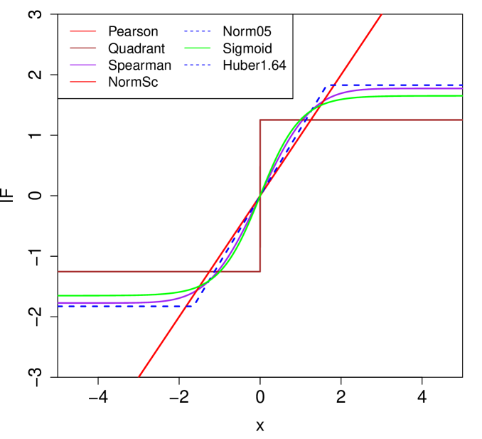
Figure 1: Location influence functions at $\rho=0$ for different transformations $g$

The influence functions of rank correlations at $F_{0}$ also factorize as in (15). Figure 1 plots these location influence functions for several choices of the transformation $g$. We see that the Pearson and normal scores correlations have the same influence function (the identity), which is unbounded. On the other hand, the IF of Huber’s $\psi_{b}$ stays constant outside the corner points $-b$ and $b$. The truncated normal scores (‘Norm05’) has the same IF as Huber’s $\psi_{b}$ provided $\alpha=\Phi(-b)$ . The Spearman rank correlation and the sigmoid transformation have smooth influence functions.

2.2 Maxbias and breakdown value

Whereas the IF measures the effect of one or a few outliers, we are now interested in the effect of a larger fraction $\varepsilon$ of contamination. For the uncontaminated distribution of the bivariate $(X,Y)$ we take the Gaussian distribution $F=F_{\rho}$ given by (9). Then we consider all contaminated distributions of the form

$$F_{H,\varepsilon}=(1-\varepsilon)F+\varepsilon H\;,$$ (16)

where $\varepsilon\geqslant 0$ and $H$ can be any distribution. This $\varepsilon$-contamination model is similar to the contaminated distributions in (10) and (20) but here $H$ is more general.

A fraction $\varepsilon$ of contamination can induce a maximum possible upward and downward bias on $T_{\psi}=\operatorname{\mbox{Cor}}(\psi(X),\psi(Y))$ denoted by

$$B^{+}(\varepsilon,T_{\psi},F)=\sup_{G\in\mathcal{F}_{\varepsilon}}(T_{\psi}(G)-T_{\psi}(F))\;\;\mbox{ and }\;\;B^{-}(\varepsilon,T_{\psi},F)=\inf_{G\in\mathcal{F}_{\varepsilon}}(T_{\psi}(G)-T_{\psi}(F))\;,$$ (17)

where $\mathcal{F}_{\varepsilon}=\{G;\;G=(1-\varepsilon)F+\varepsilon H\;\;\mbox{for any distribution }H\}$ . The proof of the following proposition is given in Section A.4 in the Supplementary Material.

Proposition 2.

Let $\varepsilon\in[0,1]$ be fixed and $\psi$ be odd and bounded. Then the maximum upward bias of $T_{\psi}$ at $F$ is given by

$$B^{+}(\varepsilon,T_{\psi},F)=\frac{(1-\varepsilon)\operatorname{\mbox{Var}}_{F}(\psi(X))\,T_{\psi}(F)+\varepsilon M^{2}}{(1-\varepsilon)\operatorname{\mbox{Var}}_{F}(\psi(X))+\varepsilon M^{2}}-T_{\psi}(F)$$ (18)

with $M:=\sup_{x}|\psi(x)|$, and the maximum downward bias is

$$B^{-}(\varepsilon,T_{\psi},F)=\frac{(1-\varepsilon)\operatorname{\mbox{Var}}_{F}(\psi(X))\,T_{\psi}(F)-\varepsilon M^{2}}{(1-\varepsilon)\operatorname{\mbox{Var}}_{F}(\psi(X))+\varepsilon M^{2}}-T_{\psi}(F)\;\;.$$ (19)

The breakdown value $\varepsilon^{*}$ of a robust estimator is loosely defined as the smallest $\varepsilon$ that can make the result useless. For instance, a location estimator $\hat{\mu}$ becomes useless when its maximal bias tends to infinity. But correlation estimates stay in the bounded range $[-1,1]$ hence the bias can never exceed 2 in absolute value, so the situation is not as clear-cut and several alternative definitions could be envisaged. Here we will follow the approach of Capéraà and Garralda (1997) who define the breakdown value of a correlation estimator as the smallest amount of contamination needed to give perfectly correlated variables a negative correlation. More precisely:

Definition 1.

Let $F$ be a bivariate distribution with $X=Y$, and $R$ be a correlation measure. Then the breakdown value of $R$ is defined as

$$\varepsilon^{*}(R)=\inf\{\varepsilon>0\;;\;\inf_{G\in\mathcal{F}_{\varepsilon}}R(G)\leqslant 0\}\;\;.$$

The breakdown value of $T_{\psi}$ then follows immediately from Proposition 2:

Corollary 1.

When $\psi$ is odd and bounded the breakdown value $\varepsilon^{*}$ of $T_{\psi}$ equals

$$\varepsilon^{*}(T_{\psi})=\frac{\operatorname{\mbox{Var}}_{F}(\psi(X))}{\operatorname{\mbox{Var}}_{F}(\psi(X))+M^{2}}\;\;.$$

The breakdown values of rank correlations were obtained in (Capéraà and Garralda, 1997; Boudt et al., 2012). They used a different contamination model, but their results still hold under $\varepsilon$-contamination as shown in Section A.5 in the Supplementary Material.

3 The proposed transformation

The change-of-variance curve (Hampel et al., 1981; Rousseeuw, 1981) is given by

$$\mbox{CVC}(z,T_{\psi},F)=\frac{\partial}{\partial\varepsilon}\left[\log V\big{(}T_{\psi},(1-\varepsilon)F+\varepsilon(\Delta_{z}+\Delta_{-z})/2\big{)}\right]|_{\varepsilon=0}$$ (20)

and measures how stable the variance of the method is when the underlying distribution is contaminated, which may make it longer tailed. We do not want the variance to grow too much, as is measured by the change-of-variance sensitivity $\kappa^{*}(T_{\psi})$, which is the supremum of the CVC. (On the other hand, negative values of the CVC indicate lower variance and are not a concern.) Since the asymptotic variance of $T_{\psi}$ satisfies $V(T_{\psi})=(V(L_{\psi}))^{2}$ we obtain $\mbox{CVC}(z,T_{\psi},F_{0})=2\,\mbox{CVC}(z,L_{\psi},\Phi)$ and $\kappa^{*}(T_{\psi})=2\,\kappa^{*}(L_{\psi})$ . Therefore we inherit all the results about the CVC from the location setting. For instance, the quadrant correlation [with $\psi(z)=\operatorname{\mbox{sign}}(z)$] has the lowest possible $\kappa^{*}(T_{\psi})$ .

Now suppose one wants to eliminate the effect of far outliers, say those that lie more than $c$ robust standard deviations away. This can be done by imposing

$$\psi(z)=0\;\;\;\mbox{whenever}\;\;\;|z|>c\;\;.$$ (21)

Such functions $\psi$ can no longer be monotone, and are called redescending instead. They were first used for M-estimation of location, and performed extremely well in the seminal simulation study of Andrews et al. (1972). They have been used in M-estimation ever since.

In the context of location estimation, Hampel et al. (1981) show that the $\psi$-function satisfying (21) with the highest efficiency subject to a given $\kappa^{*}(T_{\psi})$ is of the following form:

$$\psi_{b,c}(z)=\begin{cases}z&\mbox{ if }0\leqslant|z|\leqslant b\\ q_{1}\tanh\big{(}q_{2}(c-|z|)\big{)}\operatorname{\mbox{sign}}(z)&\mbox{ if }b\leqslant|z|\leqslant c\\ 0&\mbox{ if }c\leqslant|z|\;\;.\end{cases}$$ (22)

For any combination $0<b<c$ the values of $q_{1}$ and $q_{2}$ can be derived as in Section A.6 of the Supplementary Material. Our default choice is $b=1.5$ and $c=4$ as in Figure 2. As we will see in Table 2 this choice strikes a good compromise between robustness and efficiency. Note that the $b$ in $\psi_{b,c}$ plays the same role as the “corner value” in the Huber $\psi_{b}$ function for location estimation. In that setting, $b=1.5$ has been a popular choice from the beginning. The value $c=4$ reflects that we do not trust measurements that lie more than 4 standard deviations away. The form of $\psi_{b,c}(z)$ for $b\leqslant|z|\leqslant c$ is the result of solving a differential equation.

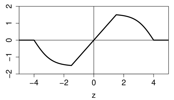
Figure 2: The proposed transformation (22) with default constants $b=1.5$ and $c=4$.

A nice property of $\psi_{b,c}$ is that under normality a large majority of the data values (in fact $86.6\%$ of them for $b=1.5$) are left unchanged by the transformation, and only a minority is modified. Leaving the majority of the data unchanged has the advantage that we keep much information about the distribution of a variable and the type of association between variables (e.g. linear), unlike rank transforms.

Figure 3: Illustration of wrapping a standardized sample $\{z_{1},\ldots,z_{n}\}$ . Values in the interval $[-b,b]$ are left unchanged, whereas values outside $[-c,c]$ are zeroed. The intermediate values are ‘folded’ inward so they still play a role.

Interestingly, $\psi_{b,c}$ pushes values between $b$ and $c$ closer to the center so intermediate outliers still play some smaller role in the correlation, whereas far outliers do not count. For this reason we refer to $\psi_{b,c}$ as the wrapping function, as it wraps the data around the interval $[-b,b]$ . Indeed, the points on the interval are mapped to themselves, whereas the other points are wrapped around the corners, as in Figure 3.

Another way to describe this is to say that wrapping multiplies the variable $z$ by a weight $w(z)$, where $w(z)\coloneqq 1$ when $|z|\leq b$ and $w(z)\coloneqq\psi_{b,c}(z)/z$ for $|z|>b$.

The influence function (15) contains $\mbox{IF}(z,L_{\psi},\Phi)=\psi_{b,c}(z)/E[\psi^{\prime}_{b,c}]$, which has the shape of $\psi_{b,c}$ in Figure 2. The bivariate influence function $\mbox{IF}((x,y),T_{\psi},F_{\rho})$ is continuous and bounded, and shown in Figure 13 in Section A.6 of the Supplementary Material.

Table 2 lists some correlation measures based on transformations $g$ that either use ranks or $\psi$-functions. For each the breakdown value $\varepsilon^{*}$ and the efficiency and gross-error sensitivity $\gamma^{*}$ at $\rho=0$ are listed. The rejection point $\delta^{*}$ says how far an outlier must lie before the IF is zero. The last column shows the product-moment correlation between a Gaussian variable $X$ and its transformed $g(X)$ . The correlation is quite high for most transformations studied here, providing insight as to why this approach works.

Table 2: Correlation measures based on transformations $g$ with their breakdown value $\varepsilon^{*}$, efficiency, gross-error sensitivity $\gamma^{*}$, rejection point $\delta^{*}$ and correlation between $X$ and $g(X)$.

$\operatorname{\mbox{Cor}}_{g}$	$\varepsilon^{*}$	eff	$\gamma^{*}$	$\delta^{*}$	Cor
Pearson	0%	100%	$\infty$	$\infty$	1
Quadrant	50%	40.5%	1.57	$\infty$	0.798
Spearman (SP)	20.6%	91.2%	3.14	$\infty$	0.977
Normal scores (NS)	12.4%	100%	$\infty$	$\infty$	1
Truncated NS, $\alpha=0.05$	16.3%	95.0%	3.34	$\infty$	0.987
Truncated NS, $\alpha=0.1$	20.7%	88.9%	2.57	$\infty$	0.971
Sigmoid	28.3%	86.6%	2.73	$\infty$	0.965
Huber, $b=\Phi^{-1}(0.95)\approx 1.64$	23.5%	95.0%	3.34	$\infty$	0.987
Huber, $b=\Phi^{-1}(0.9)\approx 1.28$	29.2%	88.9%	2.57	$\infty$	0.971
Wrapping, $b=1.5$, $c=4$	25.1%	89.0%	3.16	4.0	0.971
Wrapping, $b=1.3$, $c=4$	28.1%	84.4%	2.79	4.0	0.958

In Table 2 we see that the quadrant correlation has the highest breakdown value but the lowest efficiency. The Spearman correlation reaches a much better compromise between breakdown and efficiency. Normal scores has the asymptotic efficiency and IF of Pearson but with a breakdown value of 12.4%, a nice improvement. Truncating 5% improves its robustness a bit at the small cost of 5% of efficiency, whereas truncating 10% brings its performance close to Spearman.

Both the Huber and the wrapping correlation have a parameter $b$, the corner point, which trades off robustness and efficiency. A lower $b$ yields a higher breakdown value and a better gross-error sensitivity, but a lower efficiency. Note that the Huber correlation looks good in Table 2, but in the simulation study of Section 4 it performs less well than wrapping in the presence of outliers, and the same holds in the real data application in Section 6.2. The reason is that wrapping gives a lower weight $w(z):=\psi_{b,c}(z)/z$ to outliers and even $w(z)=0$ for $|z|>c$, whereas the Huber weight $w_{b}(z):=\psi_{b}(z)/z$ is higher for outliers and always nonzero, so even far outliers still have an effect.

Note that whenever two random variables $X$ and $Y$ are independent the correlation between the wrapped variables $g_{X}(X)$ and $g_{Y}(Y)$ is zero, even if the original $X$ and $Y$ did not satisfy any moment conditions. This follows from the boundedness of $\psi_{b,c}$ in (22).

It is well-known that the reverse is not true for the classical Pearson correlation, but that it holds when $(X,Y)$ follow a bivariate Gaussian distribution. This is also true for the wrapped correlation.

Proposition 3.

If the variables $(X,Y)$ follow a bivariate Gaussian distribution and the correlation between the wrapped variables $g_{X}(X)$ and $g_{Y}(Y)$ is zero, then $X$ and $Y$ are independent.

Another well-known property says that the Pearson correlation of a dataset $Z=\{(x_{1},y_{1}),\ldots,(x_{n},y_{n})\}$ equals 1 if and only if there are constants $\alpha$ and $\beta$ with $\beta>0$ such that

$$y_{i}=\alpha+\beta x_{i}$$ (23)

for all $i$ (perfect linear relation). The wrapped correlation satisfies a similar result.

Proposition 4.

(i) If (23) holds for all $i$ and we transform the data to $g_{X}(x_{i})=\psi_{b,c}((x_{i}-\hat{\mu}_{X})/\hat{\sigma}_{X})$ and $g_{Y}(y_{i})=\psi_{b,c}((y_{i}-\hat{\mu}_{Y})/\hat{\sigma}_{Y})$ then $\operatorname{\mbox{Cor}}(g_{X}(x_{i}),g_{Y}(y_{i}))=1$.

(ii) If $\operatorname{\mbox{Cor}}(g_{X}(x_{i}),g_{Y}(y_{i}))=1$ then (23) holds for all $i$ for which $|x_{i}-\hat{\mu}_{X}|/\hat{\sigma}_{X}\leqslant b$ and $|y_{i}-\hat{\mu}_{Y}|/\hat{\sigma}_{Y}\leqslant b$.

In part (ii) the linearity has to hold for all points with coordinates in the central region of their distribution, whereas far outliers may deviate from it. In that case the points in the central region are exactly fit by a straight line. The proofs of Propositions 3 and 4 can be found in Section A.7 of the Supplementary Material.

Remark. Whereas Proposition 3 requires bivariate gaussianity, the other results in this paper do not. In fact, Propositions 1, 2, and 4 as well as Corollary 1 still hold when the data is generated by a symmetric and unimodal distribution. The corresponding proofs in the Supplementary Material are for this more general setting.

4 Simulation Study

We now compare the correlation by transformation methods in Table 2 for finite samples. For all of these methods the correlation between two variables does not depend on any other variable in the data, so we only need to generate bivariate data here.

For the non rank-based methods we first normalize each variable by a robust scale estimate, and then estimate the location by the M-estimator with the given function $\psi$. Next we transform $x_{i}$ to $x^{*}_{i}=\psi((x_{i}-\hat{\mu}_{X})/\hat{\sigma}_{X})$ and $y_{i}$ to $y^{*}_{i}=\psi((y_{i}-\hat{\mu}_{Y})/\hat{\sigma}_{Y})$ and compute the plain Pearson correlation of the transformed sample $\{(x^{*}_{1},y^{*}_{1}),\ldots,(x^{*}_{n},y^{*}_{n})\}$.

Clean data. Let us start with uncontaminated data distributed as $F=F_{\rho}$  given by (9) where the true correlation $\rho$ ranges over $\{0,0.05,0.10,\ldots,0.95\}$. For each $\rho$ we generate $m=5000$ bivariate data sets $\bm{Z}^{j}$ with sample size $n=100$. (We also generated data with $n=20$ yielding the same qualitative conclusions.) We then estimate the bias and the mean squared error (MSE) of each correlation measure $R$ by

$$\operatorname{\mbox{bias}}_{\rho}(R)=\operatorname{\mbox{ave}}_{j=1}^{m}\left(R(\bm{Z}^{j})-\rho\right)\;\;\;\mbox{ and }\;\;\;\operatorname{\mbox{MSE}}_{\rho}(R)=\operatorname{\mbox{ave}}_{j=1}^{m}\left({R(\bm{Z}^{j})}-\rho\right)^{2}\;\;.$$ (24)

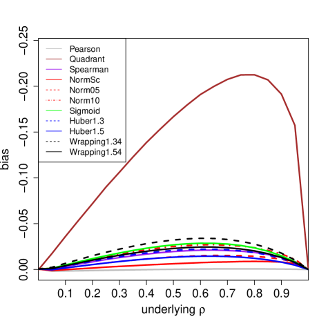
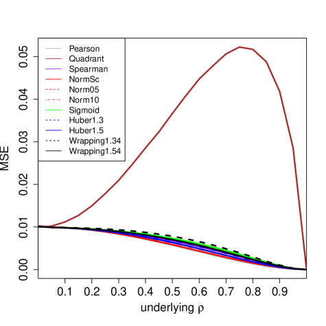
Figure 4: Bias and MSE of correlation measures based on transformation, for uncontaminated Gaussian data with sample size 100.

The bias is shown in the left part of Figure 4. The vertical axis has flipped signs because the bias was always negative, so $\rho$ is typically underestimated. Unsurprisingly, the Pearson correlation has the smallest bias (known not to be exactly zero). The normal scores correlation and the Huber $\psi$ with $b=1.5$ are fairly close, followed by truncated normal scores, Spearman and the sigmoid. Wrapping with $b=1.5$ and $b=1.3$ (both with $c=4$) comes next, still with a fairly small bias. The bias of the quadrant correlation is much higher. Note that we could have reduced the bias of all of these methods by applying the consistency function $\xi^{-1}$ of (11), which can be computed numerically. But such consistency corrections would destroy the crucial PSD property for the higher-dimensional data that motivate the present work, so we will not use them here.

The right panel of Figure 4 shows the MSE of the same methods, with a pattern similar to that of the bias. Even for $n=20$ the bias dominated the variance (not shown).

Contaminated data. In order to compare the robustness of these correlation measures we now add outliers to the data. Since the true correlation $\rho$ ranges over positive values here, we will try to bring the correlation measures down. From the proof of Proposition 2 in Section A.4 we know that the outliers have the biggest downward effect when placed at points $(k,-k)$ and $(-k,k)$ for some $k$. Therefore we will generate outliers from the distribution

$$H\;=\;\frac{1}{2}N\left(\begin{bmatrix}k\\ -k\\ \end{bmatrix},0.01^{2}I\right)+\frac{1}{2}N\left(\begin{bmatrix}-k\\ k\\ \end{bmatrix},0.01^{2}I\right)$$

for different values of $k$. The simulations were carried out for 10%, 20% and 30% of outliers, but we only show the results for 10% as the relative performance of the methods did not change much for the higher contamination levels.

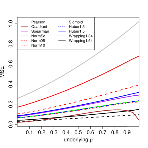
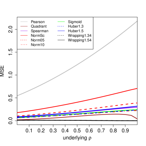
Figure 5: MSE of the correlation measures in Figure 4 with 10% of outliers placed at $k=3$ (left) and $k=5$ (right).

The results are shown in Figure 5 for $k=3$ and $k=5$. For $k=3$ we see that the Pearson correlation has by far the highest MSE, followed by normal scores (whose breakdown value of 12.4% is not much higher than the 10% of contamination). The 5% truncated normal scores and the Huber with $b=1.5$ do better, followed by the Spearman, the sigmoid, the 10% truncated normal scores and the Huber with $b=1.3$. The quadrant correlation does best among all the methods based on a monotone transformation. However, wrapping still outperforms it, because it gives the outliers a smaller weight. Even though wrapping has a slightly lower efficiency for clean data than Huber’s $\psi_{b}$ with the same $b$, in return it delivers more resistance to outliers further away from the center.

For $k=5$ the pattern is the same, except that the Pearson correlation is affected even more and wrapping has given a near-zero weight to the outliers. For $k=2$ (not shown) the contamination is not really outlying and all methods performed about the same, whereas for $k>5$ the curves of the non-Pearson correlations remain as they are for $k=5$ since all of our transformations $g$ are constant in that region.

Comparison with other robust correlation methods. As described in the introduction, several good robust alternatives to the Pearson correlation exist that do not fall in our framework. We would like to find out how well wrapping stacks up against the most well-known of them, such as Kendall’s tau. We also compare with the Gnanadesikan-Kettenring (GK) approach (5) in which we replace the variance by the square of a robust scale, in particular the MAD and the scale estimator $Q_{n}$ of Rousseeuw and Croux (1993).

For the approach starting with the estimation of a robust covariance matrix we consider the Minimum Covariance Determinant (MCD) method (Rousseeuw, 1985) using the algorithm in (Hubert et al., 2012), and the Spatial Sign Covariance Matrix (SSCM) of Visuri et al. (2000). In both cases we compute a correlation measure between variables $X_{1}$ and $X_{2}$ from the estimated scatter matrix $C$ by (6). For our bivariate generated data the matrix $C$ is only $2\times 2$, but if the original data have more dimensions the estimated correlation between $X_{1}$ and $X_{2}$ now also depends on the other variables. To illustrate this we computed the MCD and the SSCM also in $d=10$ dimensions where the true covariance matrix is given by $\Sigma_{jk}=\rho$ for $j\neq k$ and 1 otherwise. The simulation then reports the result of (6) on the first two variables only.

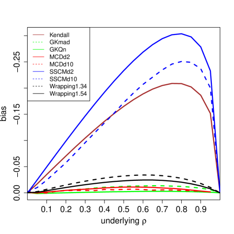
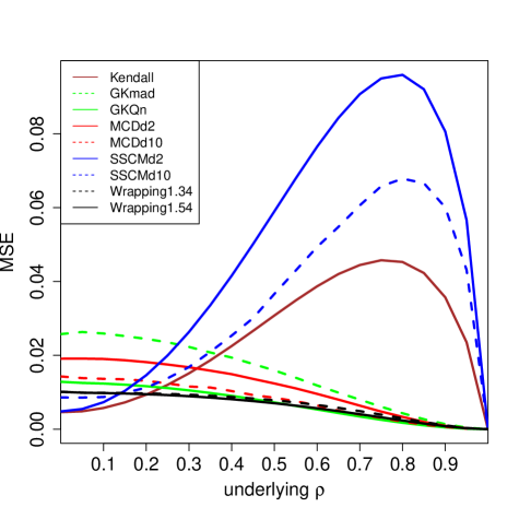
Figure 6: Bias and MSE of other robust correlation measures, for uncontaminated Gaussian data with sample size 100.

The left panel of Figure 6 shows the bias of all these methods, in the same setting as Figure 4. The two GK methods and the MCD computed in 2 and 10 dimensions have the smallest bias, followed by wrapping. The Kendall bias is substantially larger, and in fact looks similar to the bias of the quadrant correlation in Figure 6, which is not so surprising since they possess the same function $\xi(\rho)=2\arcsin(\rho)/\pi$ in (11). The bias of the SSCM is even larger, both when computed in $d=2$ dimensions and in $d=10$. The MSE in the right panel of Figure 6 shows a similar pattern.

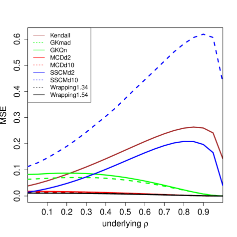
Figure 7: MSE of the correlation measures in Figure 6 with 10% of outliers placed at $k=3$ (left) and $k=5$ (right).

Figure 7 shows the effect of 10% of outliers, using the same generated data as in Figure 5. The left panel is for $k=3$. The scale of the vertical axis indicates that the outliers have increased the MSE of all methods. The MCD in $d=2$ dimensions is the least affected, whereas the GK methods, the SSCM with $d=2$ and Kendall’s tau are more sensitive. Note that the data in $d=10$ dimensions was only contaminated in the first 2 dimensions, and the MCD still does quite well in that setting. On the other hand, the MSE of the SSCM in $d=10$ is now much higher.

To conclude, wrapping holds its own even among well-known robust correlation measures outside our transformation approach. Wrapping was not the overall best method in our simulation, that would be the MCD, but the latter requires much more computation time which goes up a lot in high dimensions. Moreover, the highly robust quadrant transformation yields a low efficiency as it ignores much information in the data.

Therefore, wrapping seems a good choice for our purpose, which is to construct a fast robust method for fitting high dimensional data. Some other methods like the MCD perform better in low dimensions (say, upto 20), but in high dimensions the MCD and related methods become infeasible, whereas the SSCM does not perform well any more.

5 Use in higher dimensions

5.1 Methodology

So far the illustrations of wrapping were in the context of bivariate correlation. In this section we explain its use in the higher-dimensional context for which it was developed. Our approach is basically to wrap the data first, carry out an existing estimation technique on the wrapped data, and then use that fit for the original data. We proceed along the following steps.

Step 1: estimation. For each of the (possibly many) continuous variables $X_{j}$ with $j=1,\ldots,d$ we compute a robust initial scale estimate $\hat{\sigma}_{j}$ such as the MAD. Then we compute a one-step location M-estimator $\hat{\mu}_{j}$ with the wrapping function $\psi_{b,c}$ with defaults $b=1.5$ and $c=4$. We could take more steps or iterate to convergence, but this would lead to a higher contamination bias (Rousseeuw and Croux, 1994).

Step 2: transformation. Next we wrap the continuous variables. That is, we transform any $x_{ij}$ to

$$x_{ij}^{*}\;=\;g(x_{ij})\;=\;\hat{\mu}_{j}+\hat{\sigma}_{j}\,\psi_{b,c}\Big{(}\frac{x_{ij}-\hat{\mu}_{j}}{\hat{\sigma}_{j}}\Big{)}\;\;.$$ (25)

Note that $\operatorname{\mbox{ave}}_{i}(x^{*}_{ij})$ is a robust estimate of $\mu_{j}$ and $\operatorname{\mbox{stdev}}_{i}(x^{*}_{ij})$ is a robust estimate of $\sigma_{j}$ . The wrapped variables $X^{*}_{j}$ do not contain outliers, and when the original $X_{j}$ is Gaussian over 86% of its values remain unchanged, that is $x^{*}_{ij}=x_{ij}$ . If $x_{ij}$ is missing we have to assign a value to $g(x_{ij})$ in order to preserve the PSD property of product moment matrices, and $g(x_{ij})=\hat{\mu}_{j}$ is the natural choice. We do not transform discrete variables – depending on the context one may or may not leave them out of the subsequent analysis.

Step 3: fitting. We then fit the wrapped data $x^{*}_{ij}$ by an existing multivariate method, yielding for instance a covariance matrix or sparse loading vectors.

Step 4: using the fit. To evaluate the fit we will look at the deviations (e.g. Mahalanobis distances) of the wrapped cases $\bm{x}^{*}_{i}$ as well as the original cases $\bm{x}_{i}$ .

Note that the time complexity of Steps 1 and 2 for all $d$ variables is only $O(nd)$. Any fitting method in Step 3 must read the data so its complexity is at least $O(nd)$. Therefore the total complexity is not increased by wrapping, as illustrated in Table 1.

5.2 Estimating covariance and precision matrices

Covariance matrices. The covariance matrix of the wrapped variables has the entries

$$C(j,k)=\operatorname{\mbox{Cov}}(X^{*}_{j},X^{*}_{k})=\hat{\sigma}_{j}\,\hat{\sigma}_{k}\,\operatorname{\mbox{Cor}}\big{(}\psi_{b,c}\Big{(}\frac{x_{ij}-\hat{\mu}_{j}}{\hat{\sigma}_{j}}\Big{)},\psi_{b,c}\Big{(}\frac{y_{ik}-\hat{\mu}_{k}}{\hat{\sigma}_{k}}\Big{)}\big{)}\;.$$ (26)

for $j,k=1,\ldots,d$. The resulting matrix is clearly PSD. We also have the independence property: if variables $X_{j}$ and $X_{k}$ are independent so are $X^{*}_{j}=g(X_{j})$ and $X^{*}_{k}=g(X_{k})$, and as these are bounded their population covariance exists and is zero.

Öllerer and Croux (2015) defined robust covariances with a formula like (26) in which the correlation on the right was a rank correlation. They showed that the explosion breakdown value of the resulting scatter matrix (i.e. the percentage of outliers required to make its largest eigenvalue arbitrarily high) is at least that of the univariate scale estimator $S$ yielding $\hat{\sigma}_{j}$ and $\hat{\sigma}_{k}\,$, and their proof goes through without changes in our setting. Therefore, the robust covariance matrix (26) also has an explosion breakdown value of 50%.

The scatter matrix given by (26) is easy to compute, and can for instance be used for anomaly detection. In Section A.8 of the Supplementary Material it is illustrated how robust Mahalanobis distances obtained from the estimated scatter matrix can detect outlying cases. The scatter matrix can also be used in other multivariate methods such as canonical correlation analysis, and serve as a fast initial estimate in the computation of other robust methods such as (Hubert et al., 2012).

Precision matrices and graphical models. The precision matrix is the inverse of the covariance matrix, and allows to construct a Gaussian graphical model of the variables. Öllerer and Croux (2015) and Tarr et al. (2016) estimated the covariance matrix from rank correlations, but one could also use wrapping for this step. When the dimension $d$ is too high the estimated covariance matrix cannot be inverted, so these authors construct a sparse precision matrix by applying GLASSO. Öllerer and Croux (2015) show that the breakdown value of the resulting precision matrix, for both implosion and explosion, is as high as that of the univariate scale estimator. This remains true for wrapping, so the resulting robust precision matrix has breakdown value 50%.

5.3 Distance Correlation

There exist measures of dependence which do not give rise to PSD matrices but are used as test statistics for dependence, such as mutual information and the distance correlation of Székely et al. (2007), which yield a single nonnegative scalar that does not reflect the direction of the relation if there is one. The theory of distance correlation only requires the existence of first moments. The distance correlation dCor between random vectors $\bm{X}$ and $\bm{Y}$ is defined through the Pearson correlation between the doubly centered interpoint distances of $\bm{X}$ and those of $\bm{Y}$. It always lies between 0 and 1. The population version $\mbox{dCor}(\bm{X},\bm{Y})$ can be written in terms of the characteristic functions of the joint distribution of $(\bm{X},\bm{Y})$ and the marginal distributions of $\bm{X}$ and $\bm{Y}$. This allows Székely et al. (2007) to prove that $\mbox{dCor}(\bm{X},\bm{Y})=0$ implies that $\bm{X}$ and $\bm{Y}$ are independent, a property that does not hold for the plain Pearson correlation.

The population $\mbox{dCor}(\bm{X},\bm{Y})$ is estimated by its finite-sample version $\mbox{dCor}(\bm{X}_{n},\bm{Y}_{n})$ which is used as a test statistic for dependence. For a sample of size $n$ this would appear to require $O(n^{2})$ computation time, but there exists an $O(n\log(n))$ algorithm (Huo and Székely, 2007) for the bivariate setting.

By itself distance correlation is not robust to outliers in the data. In fact, we illustrate in Section A.9 of the Supplementary Material that the distance correlation of independent variables can be made to approach 1 by a single outlier among $100,000$ data points, and the distance correlation of perfectly dependent variables can be made to approach zero. On the other hand, we could first transform the data by the function $g$ of (25) with the sigmoid $\psi(z)=\tanh(z)$, and then compute the distance covariance. This combined method does not require the first moments of the original variables to exist, and the population version is again zero if and only if the original variables are independent (since $g$ is invertible). Figure 8 illustrates the robustness of this combined statistic.

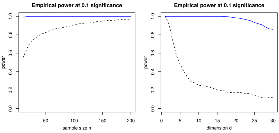
Figure 8: Left panel: power of dCor (dashed black curve) and its robust version (blue curve) for bivariate $\bm{X}$ and $\bm{Y}$ with distribution $t(1)$ and independence except for $\bm{X}_{1}=\bm{Y}_{1}$ versus the sample size $n$. Right panel: power of dCor and its robust version for $d$-dimensional $\bm{X}$ and $\bm{Y}$ with distribution $t(1)$ and $n=100$, as a function of the dimension $d$.

The data for Figure 8 were generated following Example 1(b) in (Székely et al., 2007), where $\bm{X}$ and $\bm{Y}$ are multivariate and all their components follow $t(1)$, the Student $t$-distribution with one degree of freedom. The null hypothesis states that $\bm{X}$ and $\bm{Y}$ are independent. We investigate the power of the test for dependence under the alternative that all components of $\bm{X}$ and $\bm{Y}$ are independent except for $\bm{X}_{1}=\bm{Y}_{1}$. For this we use the permutation test implemented as dcor.test in the R package energy. As in (Székely et al., 2007) we set the significance level to 0.1. The empirical power of the test is then the fraction of the $1000$ replications in which the test rejects the null hypothesis.

In the left panel of Figure 8 we see the empirical power as a function of the sample size when $\bm{X}$ and $\bm{Y}$ are both bivariate. The power of the original dCor (dashed black curve) starts around 0.6 for $n=20$ and approaches 1 when $n=200$. This indicates that for small sample sizes the components $\bm{X}_{2}$ and $\bm{Y}_{2}$, even though they are independent of everything else, have added noise in the doubly centered distances. In contrast, the power of the robust method (solid blue curve) is close to 1 overall. No outliers were added to the data, but the underlying distribution t(1) is long-tailed.

The right panel of Figure 8 shows the effect of increasing the dimension $d$ of $\bm{X}$ and $\bm{Y}$, for fixed $n=100$. At dimension $d=1$ we only have the components $\bm{X}_{1}=\bm{Y}_{1}$ and both methods have power 1. At dimension $d=2$, dCor has power 0.9 and the robust version has power 1. When increasing the dimension further, the power of dCor goes down to about 0.3 around dimension $d=8$, whereas the power of the robust method only starts going down around dimension $d=17$ and is still reasonable at dimension $d=30$. This illustrates that the transformation has tempered the effect of the $d-1$ independent variables on the doubly centered distances, delaying the curse of dimensionality in this setting.

5.4 Fast detection of anomalous cells

Wrapping is a coordinatewise approach which makes it especially robust against cellwise outliers, that is, anomalous cells $x_{ij}$ in the data matrix. In this paradigm a few cells in a row (case) can be anomalous whereas many other cells in the same row still contain useful information, and in such situations we would rather not remove or downweight the entire row. The cellwise framework was first proposed and studied by Alqallaf et al. (2002); Alqallaf et al. (2009).

Most robust techniques developed in the literature aim to protect against rowwise outliers. Such methods tend not to work well in the presence of cellwise outliers, because even a relatively small percentage of outlying cells may affect a large percentage of the rows. For this reason several authors have started to develop cellwise robust methods (Agostinelli et al., 2015). In the bivariate simulation of Section 4 we generated rowwise outliers, but the results for cellwise outliers are similar (see Section A.10 in the Supplementary Material).

Actually detecting outlying cells in data with many dimensions is not trivial, because the correlation between the variables plays a role. The DetectDeviatingCells (DDC) method of Rousseeuw and Van den Bossche (2018) predicts the value of each cell from the columns strongly correlated with that cell’s column. The original implementation of DDC required computing all $O(d^{2})$ robust correlations between the $d$ variables, yielding total time complexity $O(nd^{2})$ which grows fast in high dimensions.

Fortunately, the computation time can be reduced a lot by the wrapping method. This is because the product moment technology allows for nice shortcuts. Let us standardize two column vectors (that is, variables) $X_{n}=(x_{1},\ldots,x_{n})^{T}$ and $Y_{n}$ to zero mean and unit standard deviation. Then it is easy to verify that their correlation satisfies

$$\operatorname{\mbox{Cor}}(X_{n},Y_{n})\;=\;\frac{1}{n-1}\big{\langle}X_{n},Y_{n}\big{\rangle}\;=\;1-\frac{||X_{n}-Y_{n}||^{2}}{2(n-1)}$$ (27)

where $||\ldots||$ is the usual Euclidean distance. This monotone decreasing relation between correlation and distance allows us to switch from looking for high correlations in $d$ dimensions to looking for small distances in $n$ dimensions. When $n<<d$ this is very helpful, and used e.g. in Google Correlate (Vanderkam et al., 2013).

The identity (27) can be exploited for robust correlation by wrapping the variables first. In the (ultra)high dimensional case we can thus transpose our dataset so it becomes $d\times n$. If needed we can reduce its dimension even more to some $q<<n$ by computing the main principal components and projecting on them, which preserves the Euclidean distances to a large extent.

Finding the $k$ variables that are most correlated to a variable $X_{j}$  therefore comes down to finding its $k$ nearest neighbors in $q$-dimensional space. Fortunately there exist fast approximate nearest neighbor algorithms (Arya et al., 1998) that can obtain the $k$ nearest neighbors of all $d$ points in $q$ dimensions in $O(qd\log(d))$ time, a big improvement over $O(nd^{2})$. Note that we want to find both large positive and large negative correlations, so we look for the $k$ nearest neighbors in the set of all variables and their sign-flipped versions.

Using these shortcuts we constructed the method FastDDC which takes far less time than the original DDC and can therefore be applied to data in much higher dimensions. The detection of anomalous cells will be illustrated in the real data examples in Section 6. In both applications, finding the anomalies is the main result of the analysis.

6 Real data examples

6.1 Prostate data

In a seminal paper, Singh et al. (2002) investigated the prediction of two different types of prostate cancer from genomic information. The data is available as the R file Singh.rda in
http://www.stats.uwo.ca/faculty/aim/2015/9850/microarrays/FitMArray/data/ and contains 12600 genes. The training set consists of 102 patients and the test set has 34. There is also a response variable with the clinical classification, -1 for tumor and 1 for nontumor.

With the fast version of DDC introduced in Subsection 5.4 we can now analyze the entire genetic data set with $n=136$ and $d=12600$, which would take very long with the original DDC algorithm. Now it takes under 1 minute on a laptop. In this analysis only the genetic data is used and not the response variable, and the DDC method is not told which rows correspond to the training set. Out of the 136 rows 33 are flagged as outlying, corresponding to the test set minus one patient. The entire cellmap of size $136\times 12600$ is hard to visualize. Therefore we select the 100 variables with the most flagged cells, yielding the cellmap in Figure 9. The flagged cells are colored red when the observed value (the gene expression level) is higher than predicted, and blue when it is lower than predicted. Unflagged cells are colored yellow.

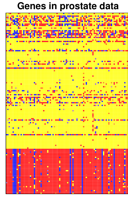
Figure 9: Prostate data: cellmap of the genes with the largest number of flagged cells.

The cellmap clearly shows that the bottom rows, corresponding to the test set, behave quite differently from the others. Indeed, it turns out that the test set was obtained by a different laboratory. This suggests to align the genetic data of the test set with that of the training set by some form of standardization, before applying a model fitted on the training data to predict the response variable on the test data.

6.2 Video data

For our second example we analyze a video of a parking lot, filmed by a static camera. The raw video can be found on http://imagelab.ing.unimore.it/visor in the category Videos for human action recognition in videosurveillance. It was originally analyzed by Ballan et al. (2009) using sophisticated computer vision technology. The video is 23 seconds long and consists of 230 Red/Green/Blue (RGB) frames of 640 by 480 pixels, so each frame corresponds with 3 matrices of size $640\times 480$. In the video we see two men coming from opposite directions, meeting in the center where they talk, and then running off one behind the other. Figure 10 shows 3 frames from the video. The men move through the scene, so they can be considered as outliers. Therefore every frame (case) is contaminated, but only in a minority of pixels (cells).

We treat the video as a dataset $\bm{X}$ with 230 row vectors $\bm{x}_{i}$ of length $921,600=640\cdot 480\cdot 3$, and we want to carry out a PCA based on the robust covariance matrix between the $921,600$ variables. When dealing with datasets this large one has to be careful with memory management, as a covariance matrix between these variables has nearly $10^{12}$ entries which is far too many to store in RAM memory. Therefore, we proceed as follows:

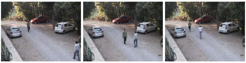
Figure 10: Frames 60, 100 and 200 of the video data.

1. Wrap the 230 data values of each RGB pixel (column) $X_{j}$ which yields the wrapped data matrix $\bm{X}^{*}$ and its centered version $\bm{Z}^{*}=\bm{X}^{*}-\bm{\overline{x^{*}}}\;$.

2. Compute the first $k=3$ loadings of $\operatorname{\mbox{Cov}}(\bm{X}^{*})=\frac{n}{n-1}\operatorname{\mbox{PM}}(\bm{Z}^{*})$ . We cannot actually compute or store this covariance matrix, so instead we perform a truncated singular value decomposition (SVD) of $\bm{Z}^{*}$ with $k=3$ components, which is mathematically equivalent. For this we use the efficient function propack:svd() from the R package svd with option neig=3, yielding the loading row vectors $\bm{v}_{j}$ for $j=1,2,3$.

3. Compute the 3-dimensional robust scores $\bm{t}_{i}$ by projecting the original data on the robust loadings obtained from the wrapped data, i.e. $\bm{t}_{i}=(\bm{x}_{i}-\bm{\overline{x^{*}}})(\bm{v}_{1}^{T},\bm{v}_{2}^{T},\bm{v}_{3}^{T})\,$.

The classical PCA result can be obtained by carrying out steps 2 and 3 on $\bm{Z}=\bm{X}-\bm{\overline{x}}\;$ without any wrapping.

We also want to compare with other robust methods. For the Spearman method we first replace each column $X_{j}$ by its ranks, i.e. $R_{ij}$ is the rank of $x_{ij}$ among all $x_{hj}$ with $h=1,\ldots,n$. We also compute $\hat{\sigma}_{j}=\operatorname{\mbox{MAD}}(X_{j})$. Then we transform each $x_{ij}$ to $\,(R_{ij}-\operatorname{\mbox{ave}}_{h}(R_{hj}))\hat{\sigma}_{j}/\operatorname{\mbox{stdev}}_{h}(R_{hj})\,$ yielding a matrix whose columns have mean zero and standard deviation $\hat{\sigma}_{j}$ to which we again apply step 2. Another method is to transform the data as in (25) but using Huber’s $\psi$ function $\psi_{b}(z)=[z]_{-b}^{b}$ with the same $b=1.5$ as in wrapping.

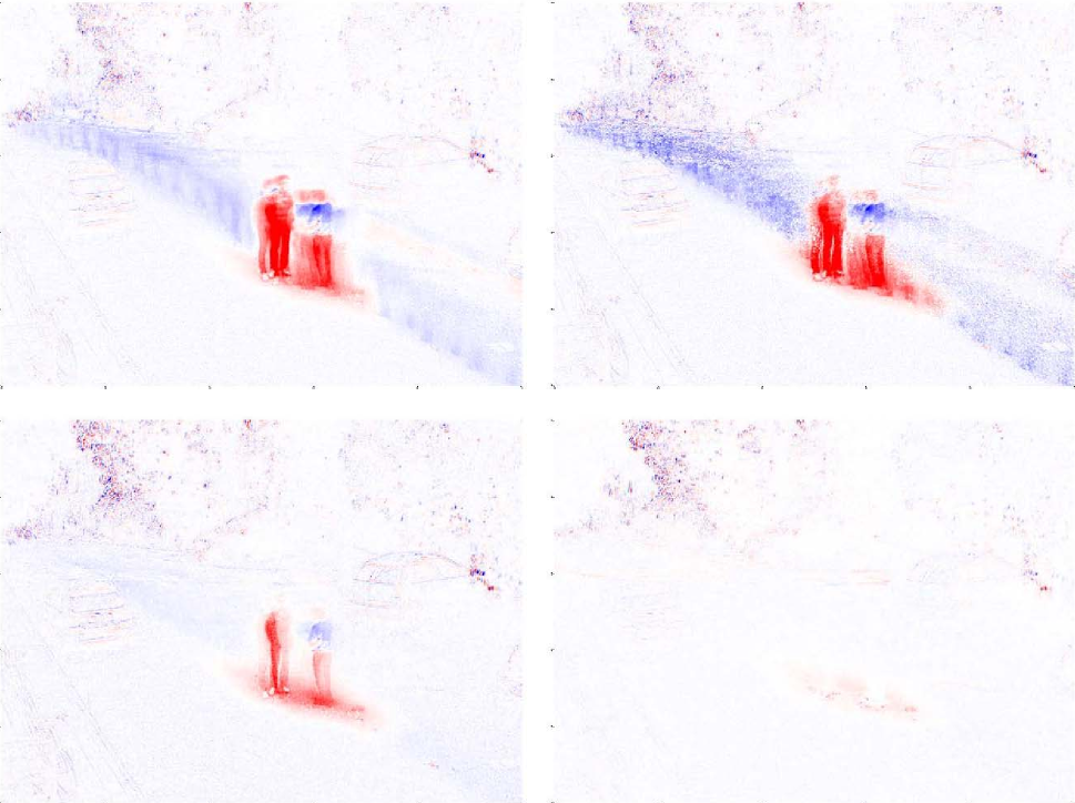
Figure 11: First loading vector of the video data, for classical PCA (upper left), Spearman correlation (upper right), Huber’s $\psi$ (lower left), and wrapping (lower right).

Figure 11 shows the first loading vector $\bm{v}_{1}$ displayed as an image, for all 4 methods considered. Positive loadings are shown in red, negative ones in blue, and loadings near zero look white. For wrapping the loadings basically describe the background, whereas for classical PCA they are affected by the moving parts (mainly the men and some leaves) that are outliers in this setting. The Spearman loadings resemble those of the classical method, whereas those with Huber’s $\psi$ are in between. Similar conclusions hold for the second and third loading vectors (not shown).

We can now compute a fit to each frame. For wrapping this is $\,\bm{\hat{x_{i}}}=\bm{t}_{i}\,(\bm{v}_{1}^{T},\bm{v}_{2}^{T},\bm{v}_{3}^{T})^{T}+\bm{\overline{x^{*}}}\,$. The residual of the frame is then $\bm{r}_{i}=\bm{x}_{i}-\bm{\hat{x_{i}}}\;$ whose 921,600 components (pixels) we can normalize by their scales. This allows us to keep those pixels of the frame where the absolute normalized residuals exceed a threshold, and turn the other pixels grey. For wrapping, this procedure yields a new video which only contains the men. This method has thus succeeded in accurately separating the movements from the background.

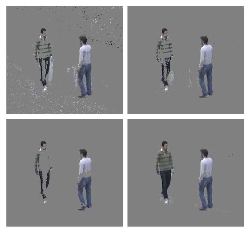
Figure 12: Residuals of the video data, for classical PCA (upper left), Spearman correlation (upper right), Huber’s $\psi$ (lower left), and wrapping (lower right).

The lower right panel of Figure 12 shows the result for the central part of frame 100. The corresponding computation for classical PCA is shown in the upper left panel, which has separated the men less well: many small elements of the background are marked as outlying, whereas parts of the man on the left are missing. We conclude that in this dataset wrapping is the most robust, classical PCA the least, and the other methods are in between.

Note that the entire analysis of this huge dataset of size 1.6 Gb in R took about two minutes on a laptop for wrapping (the times for the other three methods were similar). This is much faster than one would expect from the computation times in Table 1, which are quadratic in the dimension since they calculate the entire covariance matrix.

Of course, in real-time situations one would estimate the robust loadings on an initial set of, say, 100 frames and then process new images while they are recorded, which is very fast as it only requires a matrix multiplication. In parallel with this the robust loadings can be updated from time to time.

7 Software availability

The wrapping transform is implemented in the R package cellWise (Raymaekers et al., 2019) on CRAN, which now also provides the faster version of DDC used in the first example. The package contains two vignettes with examples. The video data of the second example, its analysis and the video with results can be downloaded fromhttps://wis.kuleuven.be/stat/robust/software .

8 Conclusions

Multivariate data often contain outlying (anomalous) values, so one needs robust methods that can detect and accommodate such outliers. The underlying assumption is that the variables are roughly Gaussian for the most part, with some possible outliers that do not follow any model and could be anywhere. (If necessary some variables can be transformed first, e.g. by taking their logarithms.)

For multivariate data in low dimensions, say up to 20, there exist robust scatter matrix estimators such as the minimum covariance determinant (MCD) method that can withstand many rowwise outliers, even those that are not visible in the marginal distributions. We recommend to use such high-breakdown methods when the dimension allows it. But in higher dimensions these methods would require infeasible computation time to achieve the same degree of robustness, and then we need to resort to other methods.

It is not easy to construct robust methods that simultaneously satisfy the independence property, yield positive semidefinite matrices, and scale well with the dimension. We achieve this by transforming the data first, after which the usual methods based on product moments are applied.

Based on statistical properties such as the influence function, the breakdown value and efficiency we selected a particular transform called wrapping. It leaves over 86% of the data intact under normality, which preserves partial information about the data distribution, granularity, and the shape of the relation between variables. Wrapping performs remarkably well in simulation. It is especially robust against cellwise outliers, where it outperforms typical rowwise robust methods. This made it possible to construct a faster version of the DetectDeviatingCells method. The examples show that the wrapping approach can deal with very high dimensional data.

Supplementary materials. These consist of a text with the proofs referenced in the paper, and an R script that illustrates the approach and reproduces the examples.

Funding. This research has been supported by projects of Internal Funds KU Leuven.

Appendix A Supplementary Material

Here the proofs of the results are collected.

A.1 Proof of Proposition 1

We can generate $(X,Y)\sim F_{p}$ for $\rho\geqslant 0$ by

$$\begin{bmatrix}X\\ Y\end{bmatrix}=A\begin{bmatrix}U\\ V\\ W\end{bmatrix}$$ (A.1)

where $U,V,W$ follow a symmetric unimodal distribution $G$ and are i.i.d., and

$$A=\begin{bmatrix}\sqrt{1-\rho}&0&\sqrt{\rho}\\ 0&\sqrt{1-\rho}&\sqrt{\rho}\end{bmatrix}.$$

For $G=N(0,1)$ the distribution of (A.1) equals (9). We now obtain $\xi(\rho)=E[\psi(u\sqrt{1-\rho}+w\sqrt{\rho})\psi(v\sqrt{1-\rho}+w\sqrt{\rho})]$. Since we are interested in $\rho\approx 0$, we can use the Taylor expansion (derived with $\delta=\sqrt{\rho}$) to obtain $\psi(u\sqrt{1-\rho}+w\sqrt{\rho})=\psi(u)+w\sqrt{\rho}\psi^{\prime}(u)+\frac{w^{2}\rho}{2}\psi^{\prime\prime}(u)+o(\rho)$ and similarly for the second factor, yielding 9 terms of which only one term remains, the others being $o(\rho)$ or zero since $\psi$ is odd:

$$\xi(\rho)=E \left[\psi(u)\left\{\psi(v)+w\sqrt{\rho}\psi^{\prime}(v)+\frac{w^{2}\rho}{2}\psi^{\prime\prime}(v)\right\}\right.$$

$$+w\sqrt{\rho}\psi^{\prime}(u)\left\{\psi(v)+w\sqrt{\rho}\psi^{\prime}(v)+\frac{w^{2}\rho}{2}\psi^{\prime\prime}(v)\right\}$$

$$+\left.\frac{w^{2}\rho}{2}\psi^{\prime\prime}(u)\left\{\psi(v)+w\sqrt{\rho}\psi^{\prime}(v)+\frac{w^{2}\rho}{2}\psi^{\prime\prime}(v)\right\}\right]$$

$$= \rho E\left[w^{2}\psi^{\prime}(u)\psi^{\prime}(v)\right]+o(\rho)$$

$$= \rho E[\psi^{\prime}(u)]E[\psi^{\prime}(v)]+o(\rho)$$

Therefore $\xi^{\prime}(0)=E[\psi^{\prime}(u)]^{2}$ and we obtain $\mbox{IF}((x,y),T,F_{0})=\psi(x)\psi(y)/E[\psi^{\prime}]^{2}$.

A.2 Influence function for general $\rho$

We first consider the non Fisher-consistent functional $T_{\psi}=E[\psi(X)\psi(Y)]$. The raw influence function of $T_{\psi}$ under the distribution $F_{\rho}$ generated as in (A.1) is then

$$\mbox{IF}_{raw}((x,y),T_{\psi},F_{\rho})=\psi(x)\psi(y)-E_{F_{\rho}}[\psi(X)\psi(Y)]\;.$$

Proof.

Let $F_{\epsilon}=(1-\epsilon)F_{\rho}+\epsilon\Delta_{(x,y)}$. Then

$$T_{\psi}(F_{\epsilon})=(1-\epsilon)E_{F_{\rho}}[\psi(X)\psi(Y)]+\epsilon E_{\Delta_{(x,y)}}[\psi(X)\psi(Y)]\;.$$

Differentiating with respect to $\epsilon$ at $\epsilon=0$ yields $-E_{F_{\rho}}[\psi(X)\psi(Y)]+\psi(x)\psi(y)$. ∎

Now denote the finite sample version of $T_{\psi}$ by $T_{n}=\frac{1}{n}\sum_{i=1}^{n}{\psi(x_{i})\psi(y_{i})}$. From the law of large numbers we have that $T_{n}$ is strongly consistent for its functional value: $T_{n}\xrightarrow{a.s.}T_{\psi}(F_{\rho})$ for $n\to\infty$. By the central limit theorem, we also have asymptotic normality of $T_{\psi}$:

$$\sqrt{n}(T_{n}-T_{\psi}(F_{\rho}))\rightarrow N(0,V_{raw})$$

where the asymptotic variance $V_{raw}$ is given by

$$V_{raw}= \;E_{\rho}[\mbox{IF}_{raw}((X,Y),T_{\psi},F_{\rho})^{2}]$$

$$= \;E_{\rho}\left[\left(\psi(X)\psi(Y)-E_{\rho}[\psi(X)\psi(Y)]\right)^{2}\right]$$

$$= \;E_{\rho}\left[\psi(X)^{2}\psi(Y)^{2}\right]-E_{\rho}[\psi(X)\psi(Y)]^{2}\;\;.$$

Now we switch to the Fisher-consistent functional $U_{\psi}(F)\coloneqq\xi^{-1}(T_{\psi}(F))$ given in (11). The general influence function defined in (12) then becomes

$$\mbox{IF}((x,y),T_{\psi},F_{\rho}):= \;\mbox{IF}_{raw}((x,y),U_{\psi},F_{\rho})$$

$$= \;\frac{\mbox{IF}_{raw}((x,y),T_{\psi},F)}{\xi^{\prime}(\rho)}$$

$$= \;\frac{\psi(x)\psi(y)-E_{\rho}[\psi(X)\psi(Y)]}{\xi^{\prime}(\rho)}$$

hence

$$\mbox{IF}((x,y),T_{\psi},F_{\rho})=\frac{\psi(x)\psi(y)-C_{\rho}}{D_{\rho}}$$ (A.2)

where $C_{\rho}\coloneqq E_{\rho}[\psi(X)\psi(Y)]$ and $D_{\rho}\coloneqq\xi^{\prime}(\rho)$ can be computed numerically to any given precision. For $\rho=0$ this simplifies to the formula in Proposition 1. Note that the influence function has the same shape for all values of $\rho$ (including $\rho=0$), only the constants $C_{\rho}$ and $D_{\rho}$ differ which amounts to shifting and rescaling the IF along the vertical axis.

Now consider the estimator $T_{n}^{*}=\xi^{-1}(T_{n})$ corresponding to the functional $U_{\psi}$ . Since $T_{n}$ is asymptotically normal, we can apply the delta method to establish the asymptotic normality of $T_{n}^{*}$ . Using $(\xi^{-1}(x))^{\prime}=1/\xi^{\prime}(\xi^{-1}(x))$ we obtain

$$\sqrt{n}(T_{n}^{*}-\rho)\rightarrow N\left(0,V\right)$$

where $V=V_{raw}/(\xi^{\prime}(\rho))^{2}$ with $V_{raw}$ as above. At $\rho=0$ this corresponds to (14).

A.3 Relation with influence functions of rank correlations

At the model distribution $F_{0}$ of (9) the influence functions of the Quadrant and Spearman correlation (Croux and Dehon, 2010) and the normal scores (Boudt et al., 2012) correspond to those of certain $\psi$-product moments. This is not a coincidence, because if we write the rank transform as $g(x_{i})=h(R_{n}(x_{i}))$ it tends to the function $\tilde{g}(x)=h(\Phi(x))$ when $n\rightarrow\infty$. If we put $\psi(x):=h(\Phi(x))$ we observe that (15) indeed holds, with $\mbox{IF}(x,h,\Phi)=h(\Phi(x))/\int{(h(\Phi))^{\prime}d\Phi}=\psi(x)/E[\psi^{\prime}]$.

For the quadrant correlation $h(u)=\operatorname{\mbox{sign}}(u-1/2)$ we get the IF of the median:

$$\mbox{IF}(x,L_{h},\Phi)=\frac{\operatorname{\mbox{sign}}(x)}{2\Phi^{\prime}(0)}=\sqrt{\frac{\pi}{2}}\operatorname{\mbox{sign}}(x)$$

and so $\gamma^{*}=\pi/2$ and $\mbox{eff}=4/\pi^{2}$.

For the normal scores rank correlation we have $h(u)=\Phi^{-1}(u)$ hence $\mbox{IF}(x,L_{h},\Phi)=x$ which is the influence function of the mean and thus unbounded, yielding $\gamma^{*}=\infty$ and $\mbox{eff}=1$. The truncated normal scores $h(u)=\Phi^{-1}\left([u]_{\alpha}^{1-\alpha}\right)=[\Phi^{-1}(u)]_{-b}^{b}$ where $\alpha=\Phi(-b)$ yields $\mbox{IF}(x,L_{h},\Phi)=\psi_{b}(x)/E[\psi_{b}^{\prime}]$, which is the influence function of Huber’s $\psi_{b}$ function.

For the Spearman correlation ($h(u)=u-1/2$) we obtain

$$\mbox{IF}(x,L_{h},\Phi)=\frac{\Phi(x)-1/2}{E[(\Phi^{\prime})^{2}]}=2\sqrt{\pi}\left(\Phi(x)-\frac{1}{2}\right)$$

which is also the influence function of the Hodges-Lehmann estimator and the Mann-Whitney and Wilcoxon tests (Hampel et al., 1986). It yields $\gamma^{*}=\pi$ and $\mbox{eff}=9/\pi^{2}$.

A.4 Proof of Proposition 2 and Corollary 1

Proof of Proposition 2. We give the proof for the maximum upward bias (the result for the maximum downward bias then follows by replacing $Y$ by $-Y$). The uncontaminated distribution of $(X,Y)$ is $F=F_{\rho}$ from (A.1). Since $\psi(X)$ and $\psi(Y)$ have the same distribution and $\psi$ is odd and bounded we find $E_{F}[\psi(X)]=E_{F}[\psi(Y)]=0$ and $E_{F}[\psi(X)^{2}]=E_{F}[\psi(Y)^{2}]$ . Now consider the contaminated distribution $G=(1-\varepsilon)F_{\rho}+\varepsilon H$ where $H$ is any distribution. At $G$ we obtain

$$\operatorname{\mbox{Cor}}_{G}(\psi(X),\psi(Y))=\frac{E_{G}[(\psi(X)-E_{G}[\psi(X)])(\psi(Y)-E_{G}[\psi(Y)])]}{\sqrt{E_{G}[(\psi(X)-E_{G}[\psi(X)]^{2})]E_{G}[(\psi(Y)-E_{G}[\psi(Y)])^{2}]}}$$

which works out to be

$$\frac{(1-\varepsilon)\operatorname{\mbox{Cov}}_{F}(U,V)+\varepsilon E_{H}[UV]-\varepsilon^{2}E_{H}[U]E_{H}[V]}{\sqrt{((1-\varepsilon)V_{F}+\varepsilon E_{H}[U^{2}]-\varepsilon^{2}E_{H}[U]^{2})((1-\varepsilon)V_{F}+\varepsilon E_{H}[V^{2}]-\varepsilon^{2}E_{H}[V]^{2})}}$$ (A.3)

where we denote $U:=\psi(X)$ and $V:=\psi(Y)$ to save space, as well as $V_{F}:=\operatorname{\mbox{Var}}_{F}(U)=E_{F}[\psi(X)^{2}]=E_{F}[\psi(Y)^{2}]=\operatorname{\mbox{Var}}_{F}(V)$.

We will show the proof for $\rho=0$ which implies that $U$ and $V$ are independent hence $\operatorname{\mbox{Cov}}_{F}(U,V)=0$ as this reduces the notation, but the proof remains valid if the term $(1-\varepsilon)\operatorname{\mbox{Cov}}_{F}(U,V)=(1-\varepsilon)V_{F}T_{\psi}(F)$ is kept. The proof consists of two parts. We first show that the contaminated correlation (A.3) is bounded from above by

$$C(\varepsilon):=\frac{\varepsilon M^{2}}{(1-\varepsilon)V_{F}+\varepsilon M^{2}}$$ (A.4)

and then we provide a sequence of contaminating distributions $H_{n}$ for which (A.3) tends to this upper bound.

1. Suppose first that $E_{H}[U]E_{H}[V]\leqslant 0$. Then we have for the numerator of (A.3):

$$E_{H}[UV]-\varepsilon E_{H}[U]E_{H}[V] \leqslant E_{H}[UV]-E_{H}[U]E_{H}[V]$$

$$\leqslant\sqrt{(E_{H}[U^{2}]-E_{H}[U]^{2})(E_{H}[V^{2}]-E_{H}[V]^{2})}\;\;.$$

Now consider the denominator of (A.3) and note that

$$\sqrt{((1-\varepsilon)V_{F}+\varepsilon(E_{H}[U^{2}]-\varepsilon E_{H}[U]^{2}))((1-\varepsilon)V_{F}+\varepsilon(E_{H}[V^{2}]-\varepsilon E_{H}[V]^{2}))}\geqslant$$

$$\sqrt{((1-\varepsilon)V_{F}+\varepsilon(E_{H}[U^{2}]-E_{H}[U]^{2}))((1-\varepsilon)V_{F}+\varepsilon(E_{H}[V^{2}]-E_{H}[V]^{2}))}$$

because $E_{H}[U^{2}]-E_{H}[U]^{2}\geqslant 0$, $E_{H}[U^{2}]\geqslant 0$, $E_{H}[U]^{2}\geqslant 0$ and $0\leqslant\varepsilon\leqslant 1$. Therefore, we can bound (A.3) from above by

$$\frac{\varepsilon\sqrt{(E_{H}[U^{2}]-E_{H}[U]^{2})(E_{H}[V^{2}]-E_{H}[V]^{2})}}{\sqrt{((1-\varepsilon)V_{F}+\varepsilon(E_{H}[U^{2}]-E_{H}[U]^{2}))((1-\varepsilon)V_{F}+\varepsilon(E_{H}[V^{2}]-E_{H}[V]^{2}))}}$$

and this quantity is maximal when $(E_{H}[U^{2}]-E_{H}[U]^{2})$ and $(E_{H}[V^{2}]-E_{H}[V]^{2})$ are as large as possible. Their supremum is in fact $M^{2}$. Therefore, (A.3) is less than or equal to (A.4).

2. Suppose now that $E_{H}[U]E_{H}[V]>0$. We will first show that the numerator is bounded as follows:

$$E_{H}[UV]-\varepsilon E_{H}[U]E_{H}[V]\leqslant\sqrt{(E_{H}[U^{2}]-\varepsilon E_{H}[U]^{2})(E_{H}[V^{2}]-\varepsilon E_{H}[V]^{2})}\;\;.$$ (A.5)

By squaring both sides we find that this is equivalent to showing

$$E_{H}[UV]^{2}-2\varepsilon E_{H}[U]E_{H}[V]E_{H}[UV]$$

$$\leqslant E_{H}[U^{2}]E_{H}[V^{2}]-\varepsilon(E_{H}[U^{2}]E_{H}[V]^{2}+E_{H}[U]^{2}E_{H}[V^{2}])$$

which is equivalent to

$$E_{H}[U^{2}]E_{H}[V^{2}]-E_{H}[UV]^{2}+\varepsilon(2E_{H}[U]E_{H}[V]E_{H}[UV]-E_{H}[U^{2}]E_{H}[V]^{2}-E_{H}[U]^{2}E_{H}[V^{2}])\geqslant 0.$$ (A.6)

We know that (A.5) holds for $\varepsilon=1$ as it is equivalent to $\operatorname{\mbox{Cov}}_{H}(U,V)\leqslant\sqrt{\operatorname{\mbox{Var}}_{H}(U)\operatorname{\mbox{Var}}_{H}(V)}$ so (A.6) is true in that case.

The general version of (A.6) with $\varepsilon\leqslant 1$ equals the LHS for $\varepsilon=1$, plus $(1-\varepsilon)$ times

$$E_{H}[U]^{2}E_{H}[V^{2}]-2E_{H}[U]E_{H}[V]E_{H}[UV]+E_{H}[U^{2}]E_{H}[V]^{2}\;\;.$$ (A.7)

Therefore, it would suffice to prove that (A.7) is nonnegative. We know that $|E_{H}[UV]|\leqslant\sqrt{E_{H}[U^{2}]E_{H}[V^{2}]}$ by Cauchy-Schwarz. Since $E_{H}[U]E_{H}[V]>0$ we obtain

$$E_{H}[U]^{2}E_{H}[V^{2}]-2E_{H}[U]E_{H}[V]E_{H}[UV]+E_{H}[U^{2}]E_{H}[V]^{2}$$

$$\geqslant E_{H}[U]^{2}E_{H}[V^{2}]-2E_{H}[U]E_{H}[V]\sqrt{E_{H}[U^{2}]E_{H}[V^{2}]}+E_{H}[U^{2}]E_{H}[V]^{2}$$

$$=\left(E_{H}[U]\sqrt{E_{H}[V^{2}]}-E_{H}[V]\sqrt{E_{H}[U^{2}]}\right)^{2}\geqslant 0\;\;.$$

Now that we have shown (A.5) we can proceed as in part 1, since (A.3) is bounded from above by

$$\frac{\varepsilon\sqrt{(E_{H}[U^{2}]-\varepsilon E_{H}[U]^{2})(E_{H}[V^{2}]-\varepsilon E_{H}[V]^{2})}}{\sqrt{((1-\varepsilon)V_{F}+\varepsilon(E_{H}[U^{2}]-\varepsilon E_{H}[U]^{2}))((1-\varepsilon)V_{F}+\varepsilon(E_{H}[V^{2}]-\varepsilon E_{H}[V]^{2}))}}$$

and this quantity is maximal when $(E_{H}[U^{2}]-\varepsilon E_{H}[U]^{2})$ and $(E_{H}[V^{2}]-\varepsilon E_{H}[V]^{2})$ are as large as possible. Their supremum is again $M^{2}$, so (A.3) is less than or equal to (A.4).

3. Now all that is left to show is that the upper bound (A.4) is sharp. Let $(k_{n})_{n\in\mathbb{N}}$ be a sequence such that $\lim_{n\to\infty}\psi(k_{n})=\sup_{x}|\psi(x)|=M$ and consider the sequence of ‘worst-placed’ contaminating distributions

$$H_{n}=\frac{1}{2}\Delta_{(k_{n},k_{n})}+\frac{1}{2}\Delta_{(-k_{n},-k_{n})}\;\;.$$ (A.8)

For the numerator of (A.3) we have $\displaystyle\lim_{n\to\infty}{\varepsilon E_{H_{n}}[UV]-\varepsilon^{2}E_{H_{n}}[U]E_{H_{n}}[V]}=\varepsilon M^{2}$ since $E_{H_{n}}[U]=0=E_{H_{n}}[V]$, and for the denominator we obtain analogously

$$\displaystyle\lim_{n\to\infty}\sqrt{((1-\varepsilon)V_{F}+\varepsilon E_{H_{n}}[U^{2}])((1-\varepsilon)V_{F}+\varepsilon E_{H_{n}}[V^{2}])}\;=\;(1-\varepsilon)V_{F}+\varepsilon M^{2}$$

so we reach the upper bound (A.4). The proof for the maximum downward bias is entirely similar, and there the worst placed contaminating distributions are of the form $H_{n}=\frac{1}{2}\Delta_{(k_{n},-k_{n})}+\frac{1}{2}\Delta_{(-k_{n},k_{n})}$ . QED.

Proof of Corollary 1. For the breakdown value we start from $F=F_{1}$ , that is $\rho=1$ and $X=Y$, so $\operatorname{\mbox{Cov}}_{F}(\psi(X),\psi(Y))=\operatorname{\mbox{Var}}_{F}(\psi(X))$ hence $T_{\psi}(F)=1$. From Proposition 2 we know that

$$\inf_{G\in\mathcal{F}_{\varepsilon}}T_{\psi}(G)=\frac{(1-\varepsilon)\operatorname{\mbox{Var}}_{F}(\psi(X))\,T_{\psi}(F)-\varepsilon M^{2}}{(1-\varepsilon)\operatorname{\mbox{Var}}_{F}(\psi(X))+\varepsilon M^{2}}\;\;.$$

For this to be nonpositive the numerator has to be, i.e. $(1-\varepsilon)\operatorname{\mbox{Var}}_{F}(\psi(X))-\varepsilon M^{2}\leqslant 0$. The smallest $\varepsilon$ for which this holds is indeed $\operatorname{\mbox{Var}}_{F}(\psi(X))/(\operatorname{\mbox{Var}}_{F}(\psi(X))+M^{2})$ . QED.

Note that we can rewrite the breakdown value as $\varepsilon^{*}=1-(E_{F}[(\psi/M)^{2}]+1)^{-1}$ so it is a strictly increasing function of $E_{F}[(\psi/M)^{2}]$. This implies that the maximizer of the breakdown value is $\psi(x)=\operatorname{\mbox{sign}}(x)$ which maximizes $E_{F}[(\psi/M)^{2}]=1$, hence $\varepsilon^{*}=0.5$ (this yields the quadrant correlation). Interestingly, the breakdown value of the scale M-estimator $S$ defined by $\operatorname{\mbox{ave}}_{i}\rho(x_{i}/S)=E_{F}[\rho]$ where $\rho(z):=\psi^{2}(z)$ is also determined by the ratio $E_{F}[\rho]/M^{2}=E_{F}[(\psi/M)^{2}]$, see e.g. Maronna et al. (2006).

A.5 Relation with breakdown values of rank correlations

The breakdown values of the rank correlations in Table 2 were derived by Capéraà and Garralda (1997) and Boudt et al. (2012), but not for the $\varepsilon$-contamination model (16). Instead they used replacement contamination, which means you can take out a certain fraction of the observations and replace them by arbitrary points. In fact $\varepsilon$-contamination is a special case of this, which corresponds to replacing a mass $\varepsilon$ distributed exactly like the original distribution $F$, whereas in general one could replace an arbitrary part of $F$. Therefore the breakdown value for replacement is always less than or equal to that for $\varepsilon$-contamination. However, in many situations the result turns out to be the same, as is the case here.

For rank correlations in the replacement model, Capéraà and Garralda (1997) and Boudt et al. (2012) showed that given a sorted sample $(x_{1},y_{1}),\ldots,(x_{n},y_{n})$ where $x_{1}<\dots<x_{n}$ and $x_{i}=y_{i}$ for all $i\in\{1,\ldots,n\}$, the worst possible bias is reached by replacing the highest and the lowest $y_{i}$ by values beyond the other end of the range.

We can in fact obtain the same type of configuration through the $\varepsilon$-contamination model. Let us start from perfectly correlated data, that is $x_{i}=y_{i}$ for all $i\in\{1,\ldots,n\}$. Then choose a sequence of contaminating distributions $H_{n}=\frac{1}{2}\Delta_{(-k_{n},k_{n})}+\frac{1}{2}\Delta_{(k_{n},-k_{n})}$ in which the $k_{n}$ are positive and tend to infinity, so the horizontal and vertical coordinates of the outliers move outside the range of the original data values. The resulting rank pairs then have the same configuration as was constructed for breakdown under replacement. Therefore the $\varepsilon$-contamination breakdown values of rank correlations equal those under replacement.

A.6 Construction of the optimal transformation

Theorem 3.1 in (Hampel et al., 1981) says that for any $0<c<\infty$ and large enough $k>0$ there exist positive constants $0<b<c$, $A$ and $B$ such that $\tilde{\psi}$ defined by

$$\tilde{\psi}(z)=\begin{cases}z&\mbox{ if }0\leqslant|z|\leqslant b\\ \sqrt{A(k-1)}\tanh\left(\frac{B}{2}\sqrt{\frac{k-1}{A}}(c-|z|)\right)\operatorname{\mbox{sign}}(z)&\mbox{ if }b\leqslant|z|\leqslant c\\ 0&\mbox{ if }c\leqslant|z|\end{cases}$$ (A.9)

satisfies

$$b=\sqrt{A(k-1)}\tanh\left(\frac{1}{2}\sqrt{\frac{(k-1)B^{2}}{A}}(c-b)\right)\;\;,$$

$A=\int_{-c}^{c}{\tilde{\psi}(x)^{2}d\Phi(x)}$ , $B=\int_{-c}^{c}{\tilde{\psi}^{\prime}(x)d\Phi(x)}$ and $\kappa^{*}(\tilde{\psi})=k$ . Theorem 4.1 then says that this function $\tilde{\psi}$ minimizes the asymptotic variance among all odd functions $\psi$ satisfying (21) subject to $\kappa^{*}(\psi)\leqslant k$, and that this optimal solution is unique (upto a positive nonzero factor). It can be verified that for a given value of $c$ there is a strictly monotone relation between $k$ and $b$, so we have decided to parametrize $\tilde{\psi}$ by the easily interpretable tuning constants $b$ and $c$. A short R-script is available that for any $b$ and $c$ derives the other constants $A$, $B$ and $k$, in turn yielding $q_{1}=\sqrt{A(k-1)}$ and $q_{2}=(B/2)\sqrt{(k-1)/A}$ . For instance, for $b=1.5$ and $c=4$ we obtain $A=0.7532528$, $B=0.8430849$ and $k=4.1517212$ hence $q_{1}=1.540793$ and $q_{2}=0.8622731$, yielding the gross-error-sensitivity $(b/B)^{2}=3.16$ and the efficiency $(B^{2}/A)^{2}=0.890$.

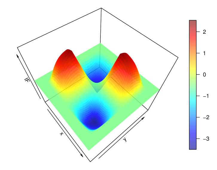
Figure 13: Influence function of $T_{\psi}$ at $F_{\rho}$ for $\rho=0.5$.

Figure 13 shows the influence function (A.2) at $\rho=0.5$ for the psi-function $\psi_{b,c}$ of (22). The influence function has the same shape at other values of $\rho$, up to shifting and rescaling the surface along the vertical axis, as shown in Section A.2.

A.7 Proof of Propositions 3 and 4

Proof of Proposition 3. It is assumed that $(X,Y)$ follows a bivariate Gaussian distribution. Due to the invariance properties of correlation, we can assume w.l.o.g. that the distribution is $F_{\rho}$ with center 0, unit variances and true correlation $-1<\rho<1$. The assumption that $\operatorname{\mbox{Cor}}(g_{X}(X),g_{Y}(Y))=0$ is equivalent to its numerator being zero, i.e. $T(F_{\rho})=E_{\rho}[\psi(X)\psi(Y)]=0$. We need to show that this implies $\rho=0$, from which independence between the components follows.

We first show that $\rho>0$ implies that $T(F_{\rho})=E_{\rho}[\psi(X)\psi(Y)]>0$. Denote $A=\{(x,y)\in\mathbb{R}^{2};\;xy>0\}$ and $B=\{(x,y)\in\mathbb{R}^{2};\;xy<0\}$. We then have:

$$E_{\rho}[\psi(X)\psi(Y)]= \int_{\mathbb{R}^{2}}{\psi(x)\psi(y)f_{\rho}(x,y)dxdy}$$

$$= \int_{A}{\psi(x)\psi(y)f_{\rho}(x,y)dxdy}+\int_{B}{\psi(x)\psi(y)f_{\rho}(x,y)dxdy}$$

$$= \int_{A}{\psi(x)\psi(y)f_{\rho}(x,y)dxdy}+\int_{A}{\psi(x)\psi(-y)f_{\rho}(x,-y)dxdy}$$

$$= \int_{A}{\psi(x)\psi(y)f_{\rho}(x,y)dxdy}-\int_{A}{\psi(x)\psi(y)f_{\rho}(x,-y)dxdy}$$

$$= \int_{A}{\psi(x)\psi(y)\left\{f_{\rho}(x,y)-f_{\rho}(x,-y)\right\}dxdy}\;.$$

In the third equality we have changed the integration variables from $(x,y)$ to $(x,-y)$. This transformation has Jacobian 1 and maps $B$ to $A$. In the fourth equality we have used that $\psi$ is odd so $\psi(-y)=-\psi(y)$. Now note that $f_{\rho}(x,y)>f_{\rho}(x,-y)$ for all $(x,y)\in A$ since $\rho>0$. We conclude that $T(F_{\rho})>0$. The proof that $T(F_{\rho})<0$ for $\rho<0$ follows by symmetry. Therefore, $T(F_{\rho})=0$ implies $\rho=0$ .

Proof of Proposition 4.

(i) From (23) and equivariance it follows that $\hat{\mu}_{Y}=\alpha+\beta\hat{\mu}_{X}$ and $\hat{\sigma}_{Y}=\beta\hat{\sigma}_{X}$ hence $g_{Y}(y_{i})=(y_{i}-\hat{\mu}_{Y})/\hat{\sigma}_{Y}=(x_{i}-\hat{\mu}_{X})/\hat{\sigma}_{X}=g_{X}(x_{i})$ for all $i$.

(ii) From $\operatorname{\mbox{Cor}}(g_{X}(x_{i}),g_{Y}(y_{i}))=1$ and $\operatorname{\mbox{ave}}_{i}(g_{X}(x_{i}))=0$ and $\operatorname{\mbox{ave}}_{i}(g_{Y}(y_{i}))=0$ it follows that there is a constant $\gamma>0$ such that $g_{Y}(y_{i})=\gamma g_{X}(x_{i})$ for all $i$. For the $i$ for which $|x_{i}-\hat{\mu}_{X}|/\hat{\sigma}_{X}\leqslant b$ and $|y_{i}-\hat{\mu}_{Y}|/\hat{\sigma}_{Y}\leqslant b$ it holds that $g_{Y}(y_{i})=(y_{i}-\hat{\mu}_{Y})/\hat{\sigma}_{Y}$ and $g_{X}(x_{i})=(x_{i}-\hat{\mu}_{X})/\hat{\sigma}_{X}$ hence $(y_{i}-\hat{\mu}_{Y})/\hat{\sigma}_{Y}=\gamma(x_{i}-\hat{\mu}_{X})/\hat{\sigma}_{X}$ which implies (23) with $\alpha=\hat{\mu}_{Y}-\gamma\hat{\mu}_{X}\hat{\sigma}_{Y}/\hat{\sigma}_{X}$ and $\beta=\gamma\hat{\sigma}_{Y}/\hat{\sigma}_{X}$.

A.8 Illustration of anomaly detection based on robust location and scatter

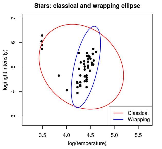
Figure 14: Plot of the 47 stars with their classical tolerance ellipse (red) and the one based on wrapped covariance (blue).

To visualize things we consider a small bivariate data set, about the star cluster CYG OB1 consisting of 47 stars in the direction of Cygnus. Their Hertzsprung-Russell diagram is a plot of the logarithm of each star’s light intensity versus the logarithm of its temperature. The data can be found on page 27 of (Rousseeuw and Leroy, 1987) and is plotted in Figure 14. We see that the majority of the stars (the so-called main sequence stars) follows a certain upward trend, whereas there are four anomalous stars in the upper left corner. These are red giant stars. In this data set the anomalies are measured correctly, but they belong to a different population.

The classical correlation between the variables is $-0.21$ which would indicate a negative relation. However, this decreasing trend is caused by the four outliers, and without them the trend would be increasing. Indeed, the wrapped correlation is $0.57$ indicating a positive relation. Figure 14 shows the $99\%$ tolerance ellipse derived from the classical mean and covariance matrix, in red. The four outliers have pulled the ellipse toward them, making them lie on its boundary. In contrast, the tolerance ellipse from the wrapped mean and covariance (in blue) fits the majority of the stars, leaving aside the four outliers.

Of course, in higher dimensions we can no longer plot the data points or draw the tolerance ellipsoids. But in that case we can still look at the classical Mahalanobis distance of each case $\bm{x}_{i}$ given by

$$\mbox{MD}(\bm{x}_{i})=\sqrt{(\bm{x}_{i}-\hat{\bm{\mu}})^{\prime}\hat{\bm{\Sigma}}^{-1}(\bm{x}_{i}-\hat{\bm{\mu}})}\;\;,$$ (A.10)

in which $\hat{\bm{\mu}}$ is the arithmetic mean and $\hat{\bm{\Sigma}}$ the empirical covariance matrix. The left panel of Figure 15 plots $\mbox{MD}(\bm{x}_{i})$ versus the case number $i$. In this plot the four giant stars lie close to the cutoff value $\sqrt{\chi^{2}_{d,0.99}}$ for dimension $d=2$. But they are easily detected in the right hand panel, which plots the robust distances given by (A.10) where this time $\hat{\bm{\mu}}$ and $\hat{\bm{\Sigma}}$ are the location and scatter matrix obtained from the wrapped data. These robust estimates have thus allowed us to detect the anomalies.

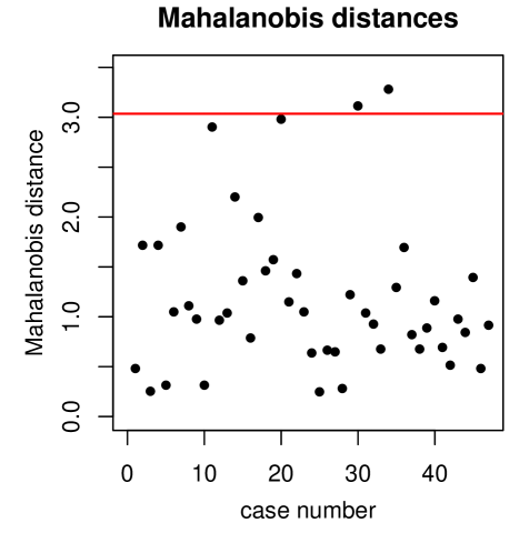
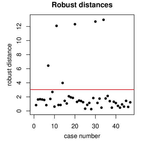
Figure 15: Classical distances of the stars (left) and their robust distances based on wrapped location and covariance (right).

A.9 Distance correlation after transformation

The distance correlation dCor between random vectors $\bm{X}$ and $\bm{Y}$ is defined by the Pearson correlation between the doubly centered interpoint distances of $\bm{X}$ and those of $\bm{Y}$ (Székely et al., 2007). It always lies between 0 and 1. Interestingly, $\mbox{dCor}(\bm{X},\bm{Y})$ can also be written in terms of the characteristic functions of the joint distribution of $(\bm{X},\bm{Y})$ and the marginal distributions of $\bm{X}$ and $\bm{Y}$. Using this result Székely et al. (2007) prove that $\mbox{dCor}(\bm{X},\bm{Y})=0$ implies that $\bm{X}$ and $\bm{Y}$ are independent, which is not true for the plain Pearson correlation (except for multivariate Gaussian data).

The population $\mbox{dCor}(\bm{X},\bm{Y})$ is estimated by its finite-sample version $\mbox{dCor}(\bm{X}_{n},\bm{Y}_{n})$ which is a test statistic for dependence. Unfortunately this statistic is very sensitive to outliers. To illustrate this we first generate $n=100,000$ data points from the standard bivariate Gaussian distribution, which has $\mbox{dCor}(\bm{X},\bm{Y})=0$, and replace a single observation by an outlier in the point $(a,a)$. The left panel of Figure 16 shows $\mbox{dCor}(\bm{X}_{n},\bm{Y}_{n})$ as a function of $a$. For this we used the fast algorithm of Huo and Székely (2007) as implemented in the function dcor2d in the R package energy, which can handle such a large sample size $n$. For $a=0$ we obtain $\mbox{dCor}(\bm{X}_{n},\bm{Y}_{n})\approx 0$ but by letting $a$ increase we can bring the result close to 1, even though the remaining $99,999$ points were generated independently.

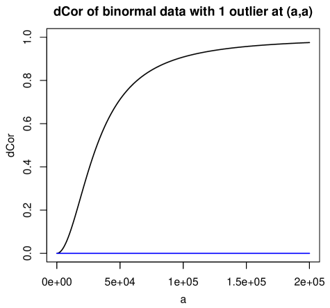
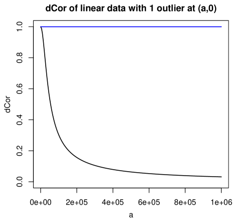
Figure 16: Left panel: distance correlation (black curve) and its robust version (blue curve) of a data set with $99,999$ standard Gaussian data points and one outlier at $(a,a)$ versus $a$. Right panel: distance correlation of data with $99,999$ data points $(x_{i},x_{i})$ with standard Gaussian $x_{i}$ and one outlier at $(a,0)$.

We can also do the opposite, by starting from a perfectly dependent setting. For this we generate $\bm{X}_{n}$ from the univariate standard Gaussian distribution, and take $\bm{Y}_{n}\,:=\,\bm{X}_{n}$ so that $\mbox{dCor}(\bm{X}_{n},\bm{Y}_{n})=1$. Then we replace a single observation by an outlier in the point $(a,0)$. In the right panel of Figure 16 we now see that we can bring $\mbox{dCor}(\bm{X}_{n},\bm{Y}_{n})$ close to 0 by this single outlier out of $100,000$ data points.

We now apply our methodology of first transforming the individual variables. For this we use the function $g$ of (25) where $\hat{\mu}_{j}$ is the sample median and $\hat{\sigma}_{j}$ is the median absolute deviation. For the $\psi$-function we use the sigmoid $\psi(z)=\tanh(z)$. After this transformation we compute the distance correlation. This combined method no longer requires the first moments of the original variables to exist because $\psi$ is bounded, and its population version is again zero if and only if the original $\bm{X}$ and $\bm{Y}$ are independent, since $\psi$ is invertible. The blue lines in Figure 16 are the result of applying the combined method, which by construction is insensitive to the outlier.

The robustness of the proposed method can help even when no outliers are added but distributions are long-tailed, as illustrated in Figure 8.

A.10 Simulation with cellwise outliers

This section repeats the simulation in Section 4 for cellwise outliers. The clean data are exactly the same, but now we randomly select data cells and replace them by outliers following the distribution $N(k,0.01^{2})$ when they occur in the $x$-coordinate and $N(-k,0.01^{2})$ when they occur in the $y$-coordinate. The simulation was run for 10%, 20% and 30% of cellwise outliers, but the patterns were similar across contamination levels.

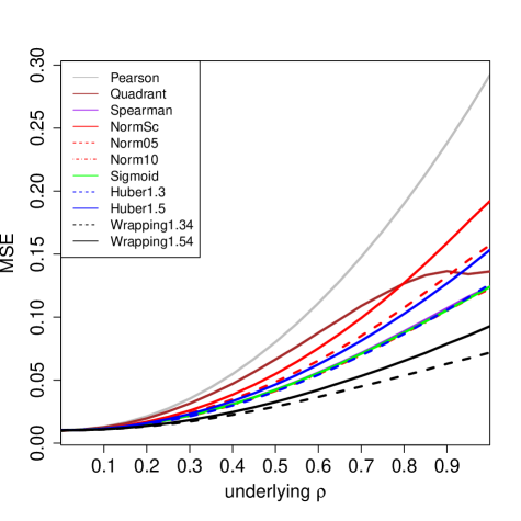
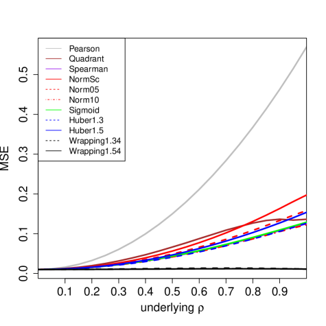
Figure 17: MSE of the correlation measures in Figure 4 with 10% of cellwise outliers placed with $k=3$ (left) and $k=5$ (right).

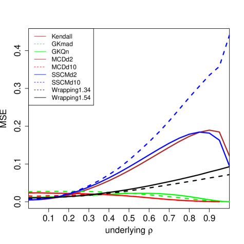
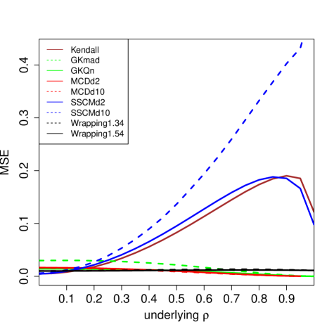
Figure 18: MSE of the correlation measures in Figure 6 with 10% of cellwise outliers placed with $k=3$ (left) and $k=5$ (right).

Figure 17 shows the MSE of the same transformation-based correlation measures as in Figure 4, with 10% of cellwise outliers for $k=3$ and $k=5$. Within this class Pearson again has the worst MSE, followed by normal scores. The quadrant correlation is next, and does not look as good here as for rowwise outliers. Wrapping has the lowest MSE, and again outperforms Spearman, sigmoid and Huber because it moves the outlying cells to the central part of their variable.

Figure 18 compares wrapping to the correlation measures in Figure 7 in the presence of these cellwise outliers. Also here the SSCM has the largest bias, especially in $d=10$ dimensions, followed by Kendall’s tau. Wrapping does well but not as well as MCD and GK when $k=3$, and their performance is similar for $k=5$. But in higher dimensions wrapping still has the redeeming feature that it yields a PSD correlation matrix unlike the GK method, whereas the MCD suffers from the propagation of cellwise outliers and a high computation time.

References

- Agostinelli et al. (2015) Agostinelli, C., A. Leung, V. J. Yohai, and R. H. Zamar (2015). Robust estimation of multivariate location and scatter in the presence of cellwise and casewise contamination. Test 24(3), 441–461.
- Alqallaf et al. (2002) Alqallaf, F., K. Konis, R. D. Martin, and R. H. Zamar (2002). Scalable robust covariance and correlation estimates for data mining. In Proceedings of the Eighth ACM SIGKDD International Conference on Knowledge Discovery and Data Mining, KDD ’02, New York, NY, USA, pp. 14–23. ACM.
- Alqallaf et al. (2009) Alqallaf, F., S. Van Aelst, V. J. Yohai, and R. H. Zamar (2009). Propagation of outliers in multivariate data. The Annals of Statistics 37(1), 311–331.
- Andrews et al. (1972) Andrews, D. F., P. J. Bickel, F. R. Hampel, P. J. Huber, W. H. Rogers, and J. W. Tukey (1972). Robust Estimates of Location: Survey and Advances. Princeton University Press.
- Arya et al. (1998) Arya, S., D. M. Mount, N. S. Netanyahu, R. Silverman, and A. Y. Wu (1998). An optimal algorithm for approximate nearest neighbor searching in fixed dimensions. Journal of the ACM 45(6), 891–923.
- Ballan et al. (2009) Ballan, L., M. Bertini, A. Del Bimbo, L. Seidenari, and G. Serra (2009). Effective codebooks for human action categorization. In Proceedings of ICCV International Workshop on Video-oriented Object and Event Classification, Kyoto, Japan, pp. 506–513.
- Boudt et al. (2012) Boudt, K., J. Cornelissen, and C. Croux (2012). The Gaussian rank correlation estimator: robustness properties. Statistics and Computing 22(2), 471–483.
- Capéraà and Garralda (1997) Capéraà, P. and A. I. Garralda (1997). Taux de résistance des tests de rang d’indépendance. The Canadian Journal of Statistics 25(1), 113–124.
- Croux and Dehon (2010) Croux, C. and C. Dehon (2010). Influence functions of the Spearman and Kendall correlation measures. Statistical Methods & Applications 19(4), 497–515.
- Gnanadesikan and Kettenring (1972) Gnanadesikan, R. and J. Kettenring (1972). Robust estimates, residuals, and outlier detection with multiresponse data. Biometrics 28, 81–124.
- Hampel et al. (1986) Hampel, F., E. Ronchetti, P. J. Rousseeuw, and W. Stahel (1986). Robust Statistics: The Approach Based on Influence Functions. New York: Wiley.
- Hampel et al. (1981) Hampel, F., P. J. Rousseeuw, and E. Ronchetti (1981). The change-of-variance curve and optimal redescending M-estimators. Journal of the American Statistical Association 76, 643–648.
- Huber (1981) Huber, P. (1981). Robust Statistics. New York: Wiley.
- Hubert et al. (2012) Hubert, M., P. J. Rousseeuw, and T. Verdonck (2012). A deterministic algorithm for robust location and scatter. Journal of Computational and Graphical Statistics 21, 618–637.
- Huo and Székely (2007) Huo, X. and G. J. Székely (2016). Fast computing for distance covariance. Technometrics 58, 435–447.
- (16) Khan, J., S. Van Aelst, and R. H. Zamar (2007). Robust linear model selection based on least angle regression. Journal of the American Statistical Association 102, 1289–1299.
- Maronna et al. (2006) Maronna, R., D. Martin, and V. Yohai (2006). Robust Statistics: Theory and Methods. New York: Wiley.
- Maronna and Zamar (2002) Maronna, R. and R. Zamar (2002). Robust estimates of location and dispersion for high-dimensional data sets. Technometrics 44, 307–317.
- Öllerer and Croux (2015) Öllerer, V. and C. Croux (2015). Robust high-dimensional precision matrix estimation. In K. Nordhausen and S. Taskinen (Eds.), Modern Nonparametric, Robust and Multivariate Methods, pp. 325–350. Cham: Springer International Publishing.
- Raymaekers et al. (2019) Raymaekers, J., P. J. Rousseeuw, W. Van den Bossche, and M. Hubert (2019). cellWise: Analyzing Data with Cellwise Outliers. R package 2.1.0, CRAN.
- Rousseeuw (1981) Rousseeuw, P. J. (1981). A new infinitesimal approach to robust estimation. Zeitschrift für Wahrscheinlichkeitstheorie und Verwandte Gebiete 56(1), 127–132.
- Rousseeuw (1984) Rousseeuw, P. J. (1984). Least median of squares regression. Journal of the American Statistical Association 79, 871–880.
- Rousseeuw (1985) Rousseeuw, P. J. (1985). Multivariate estimation with high breakdown point. In W. Grossmann, G. Pflug, I. Vincze, and W. Wertz (Eds.), Mathematical Statistics and Applications, Vol. B, pp. 283–297. Dordrecht: Reidel Publishing Company.
- Rousseeuw and Croux (1993) Rousseeuw, P. J. and C. Croux (1993). Alternatives to the median absolute deviation. Journal of the American Statistical Association 88, 1273–1283.
- Rousseeuw and Croux (1994) Rousseeuw, P. J. and C. Croux (1994). The bias of k-step M-estimators. Statistics & Probability Letters 20, 411–420.
- Rousseeuw and Leroy (1987) Rousseeuw, P. J. and A. Leroy (1987). Robust Regression and Outlier Detection. New York: Wiley.
- Rousseeuw and Ronchetti (1981) Rousseeuw, P. J. and E. Ronchetti (1981). Influence curves of general statistics. Journal of Computational and Applied Mathematics 7(3), 161–166.
- Rousseeuw and Van den Bossche (2018) Rousseeuw, P. J. and W. Van den Bossche (2018). Detecting deviating data cells. Technometrics 60, 135–145.
- Shevlyakov and Oja (2016) Shevlyakov, G. and H. Oja (2016). Robust Correlation: Theory and Applications. New York: Wiley.
- Singh et al. (2002) Singh, D., P. Febbo, K. Ross, D. Jackson, J. Manola, C. Ladd, P. Tamayo, A. Renshaw, A. D’Amico, J. Richie, E. Lander, M. Loda, P. Kantoff, T. Golub, and W. Sellers (2002). Gene expression correlates of clinical prostate cancer behavior. Cancer Cell 1, 203–209.
- Spearman (1904) Spearman, C. (1904). General intelligence, objectively determined and measured. The American Journal of Psychology 15(2), 201–292.
- Székely et al. (2007) Székely, G. J., M. L. Rizzo and N. K. Bakirov (2007). Measuring and testing dependence by correlation of distances. The Annals of Statistics 35, 2769–2794.
- Tarr et al. (2016) Tarr, G., S. Muller, and N. Weber (2016). Robust estimation of precision matrices under cellwise contamination. Computational Statistics and Data Analysis 93, 404 – 420.
- Vanderkam et al. (2013) Vanderkam, S., R. Schonberger, H. Rowley, and S. Kumar (2013). Nearest Neighbor Search in Google Correlate. Google. http://www.google.com/trends/correlate/nnsearch.pdf.
- Visuri et al. (2000) Visuri, S., V. Koivunen, and H. Oja (2000). Sign and rank covariance matrices. Journal of Statistical Planning and Inference 91, 557–575.