Matter distribution and spin-orbit force in spherical nuclei

Abstract

We investigate the possibility that some nuclei show density distributions with a depletion in the center, a semi-bubble structure, by using a Hartree-Fock plus Bardeen-Cooper-Schrieffer approach. We separately study the proton, neutron and matter distributions in 37 spherical nuclei mainly in the $s-d$ shell region. We found a relation between the semi-bubble structure and the energy splitting of spin-orbit partner single particle levels. The presence of semi-bubble structure reduces this splitting, and we study its consequences on the excitation spectrum of the nuclei under investigation by using a quasi-particle random-phase-approximation approach. The excitation energies of the low-lying $4^{+}$ states can be related to the presence of semi-bubble structure in nuclei.

I Introduction

The matter distribution of atomic nuclei is ruled by the interplay between the attraction of the nucleon-nucleon interaction and the repulsion induced by the Pauli exclusion principle and the Coulomb force. Since the short range of the interaction saturates the attraction effect, the global results is an almost constant matter distribution in the nuclear interior. This picture describes correctly the great majority of nuclei. However, there is a possibility that, in some cases, repulsive effects dominate and, consequently, they produce a central depression in the matter distribution that in the literature has taken the name of bubble won72 . Following a commonly adopted nomenclature, we call semi-bubble (SB) the nuclear systems with central depressions, since with the term bubble is commonly called a distribution which is exactly zero at the center dec03 .

The possibility that some nuclei present a SB structure in the proton, neutron or matter distribution, is a problem which has been widely investigated by using various nuclear models (see, for example dav72 ; cam73 ; fri86 ; kha08 ; gra09 ; chu10 ; wan11 ; yao12 ; meu14 ; li16 ; dug17 ; sch17 ). In nuclei with a large number of protons, i. e. heavy and super-heavy nuclei, the SB features of the distributions are mainly due to the Coulomb repulsion whose effects become relevant sch17 . In this article, we address our attention to medium-heavy nuclei in the $s-d$ shell region where the source of eventual SB structures is related to the Pauli principle.

The best experimental tool to investigate matter distributions is the elastic electron scattering, even though it is mainly sensitive to the charge density bof96 . These type of experiments can reach a sufficiently high resolution power to allow the direct identification of SB structures. Unfortunately, the nuclei where SB proton distributions have been predicted are unstable, therefore they cannot be used as targets in traditional scattering experiments. The facilities ELISe at FAIR sim07 and SCRIT at RIKEN sud09 are devised to carry out electron scattering experiments on unstable nuclei. They use different techniques and will become operative in the near future.

The technical difficulties outlined above have stimulated the search for secondary, measurable, effects induced by, or directly related to, the SB distributions. In all the mean-field (MF) descriptions of the nucleus, the effects on the total and single particle (s.p.) energies of the spin-orbit (s.o.) force are related to the derivatives of the matter, proton and neutron distributions. The usual behavior of these distributions makes these derivatives to be almost zero in the nuclear interior, and negative on the surface. The presence of a SB structure generates a positive derivative term in the nuclear interior, and consequently a reduction of the effects of the s.o. force that could be observed by measuring the energy difference between s.o. partner levels in transfer reactions bur11t ; bur14 or in sophisticated gamma ray detection experiments mut15t ; mut17 . This modification changes also the excitation spectrum. We have investigated wether the comparison of spectra of isotopic or isotonic nuclei allows to identify the presence of a SB in proton or neutron densities.

As already pointed out, in this article we investigate nuclei in the $s-d$ region of the nuclear chart to identify those which show a SB proton, neutron or matter distribution, and the eventual consequences of this feature. Since deformation can mask the effects induced by the SB structure, we have considered only spherical nuclei.

In our investigation we have used the Hartree-Fock (HF) plus Bardeen-Cooper-Schrieffer (BCS) approach to describe the ground state of the nuclei we have studied ang14 . In this way, pairing effects are taken into account in open shell nuclei. The excited states have been described by using a Quasi-particle Random Phase Approximation (QRPA) approach don17 . Our calculations have been carried out by consistently using the same effective nucleon-nucleon interaction in each of the three steps, HF, BCS and QRPA. We have used four different finite-range interactions of Gogny type, with and without tensor terms, in order to identify effects independent of the specific input of the calculations.

We present in Sec. II the features of our HF+BCS+QRPA approach interesting for the present study. The following sections are dedicated to the presentation of the results. In Sec. III we compare the performances of our approach in the description of the binding energies of the nuclei under investigation. In Sec. IV we identify those nuclei showing SB structures. We investigate separately the proton, neutron and matter distributions and we relate them to the shell structure generated by the four nucleon-nucleon interactions we have considered. In Sec. V we analyze the link between SB densities and the energy splitting between s.o. partner levels. In Sec. VI we investigate the excitation spectra of some SB nuclei to identify effects related to changes in the s.o. energy splitting. A summary of our results is given in Sec. VII where we also draw our conclusions.

II The theoretical model

We describe the ground states of the nuclei we have investigated by using a HF+BCS approach. In Refs. ang14 ; ang15 ; ang16a , we showed that our HF+BCS calculations produce results very closed to those obtained with the better grounded Hartree-Fock-Bogoliubov (HFB) theory. For the purposes of the present investigation, the differences between the results of the two approaches are not relevant.

The HF+BCS s.p. wave functions and the corresponding occupation numbers have been used to describe the excited states within the QRPA theory presented in detail in Ref. don17 . In this reference we established the criteria for the numerical stability of all the three steps of our calculations. In the present study we have adopted the same criteria also for those nuclei which we investigate here for the first time.

A crucial feature of our approach is the consistent use of the same finite-range interaction in each of the three steps of our calculations. We have chosen to work with four different finite-range interactions. One of them is the traditional D1S Gogny force ber91 , widely used in the literature, whose parameter values were chosen to reproduce the experimental values of a large set of binding energies and charge radii of nuclei belonging to various regions of the nuclear chart. However, this force has a well know drawback: the neutron matter equation of state has an unphysical behavior at large densities cha08 . To solve this problem, the D1M parameterization was proposed cha07t ; gor09 This is the second interaction we have considered.

Together with these two parameterizations we have used the D1ST2a and the D1MTd forces, both containing tensor and tensor-isospin terms, and constructed by following the strategy discussed in Refs. ang12 ; gra13 ; ang16a . Starting with the original D1S and D1M parameterizations, respectively, we added two tensor terms of the form

$$V_{\rm T}(1,2)=\left[{\cal V}_{\rm T1}+{\cal V}_{\rm T2}\mbox{\boldmath$\tau$}(1)\cdot\mbox{\boldmath$\tau$}(2)\right]S_{12}\,\exp\left[-{({\bf r}_{1}-{\bf r}_{2})^{2}/\mu_{\rm T}}\right]\,,$$ (1)

where we have indicated with $\tau$ the isospin of the nucleon, and with $S_{12}$ the traditional tensor operator bla52 . A proper formulation of a new force would imply a global refit. However, since the observables used to choose the values of the D1S and D1M parameters are essentially insensitive to the tensor force, we maintained the original parameterizations of the central channels and selected the values of the parameters of the tensor force, ${\cal V}_{\rm T1}$ and ${\cal V}_{\rm T2}$, in the following way: for the D1ST2a they were chosen in order to reproduce the excitation energy of the $0^{-}$ state in ¹⁶O and the energy splitting of the neutron $1f$ s.p. levels in ⁴⁸Ca (see Ref. ang12 ), and for the D1MTd to properly describe the excitation energies of the $0^{-}$ states in ¹⁶O and in ⁴⁸Ca. These two nuclei are representative of the nuclear chart regions we want to investigate, and the $0^{-}$ excited states and the splitting of spin orbit partners are extremely sensitive to the tensor force ang11 . In both interactions the value of $\mu_{\rm T}$ has been chosen to be equal to that of the Gaussian with the longest range in the D1S and D1M interactions, respectively (see Table 1).

	${\cal V}_{\rm T1}$ (MeV)	${\cal V}_{\rm T2}$ (MeV)	$\mu_{\rm T}$ (fm)
D1ST2a	-135.0	115.0	1.2
D1MTd	-230.0	180.0	1.0

Table 1: Values of the parameters of the tensor force, defined in Eq.(1),
for the D1ST2a and D1MTd interactions.

Comparing the results obtained with these four interactions, we have disentangled effects independent of the only arbitrary input of our approach the effective nucleon-nucleon force. On the other hand, the main aim of our study is the relation between the presence of SB in the matter, proton and neutron distributions and the energy splitting of s.o. partner levels, which is rather sensitive to $V_{\rm T}$ ots06 ; therefore a comparison of results obtained with and without tensor terms in the interaction is mandatory.

In this study we have investigated 37 nuclei having even $Z$ values between 8 and 26 and listed in Table 2. All these nuclei are spherical, according to the axially deformed HFB calculations of Refs. cea ; ang01a , thus avoiding the possible complications that deformation would produce in the identification of SB structures.

element	$A$	D1M	D1S	D1MTd	D1ST2a	exp		element	$A$	D1M	D1S	D1MTd	D1ST2a	exp
O	$16$	$-7.98$	$-8.11$	$-8.03$	$-8.10$	$-7.98$		Ar	$38$	$-8.52$	$-8.63$	$-8.58$	$-8.63$	$-8.61$
	$18$	$-7.72$	$-7.85$	$-7.79$	$-7.86$	$-7.77$			$40$	$-8.46$	$-8.57$	$-8.51$	$-8.55$	$-8.60$
	$20$	$-7.54$	$-7.66$	$-7.62$	$-7.68$	$-7.57$		Ca	$34$	$-7.15$	$-7.26$	$-7.21$	$-7.26$	$-7.20$
	$22$	$-7.30$	$-7.41$	$-7.38$	$-7.44$	$-7.37$			$36$	$-7.76$	$-7.87$	$-7.82$	$-7.87$	$-7.82$
	$24$	$-6.94$	$-7.04$	$-7.03$	$-7.08$	$-7.04$			$38$	$-8.18$	$-8.30$	$-8.24$	$-8.30$	$-8.24$
Ne	$26$	$-7.59$	$-7.69$	$-7.59$	$-7.61$	$-7.75$			$40$	$-8.51$	$-8.63$	$-8.57$	$-8.63$	$-8.55$
	$28$	$-7.24$	$-7.34$	$-7.27$	$-7.30$	$-7.39$			$42$	$-8.56$	$-8.67$	$-8.62$	$-8.67$	$-8.62$
	$30$	$-6.92$	$-7.01$	$-6.97$	$-7.00$	$-7.04$			$44$	$-8.60$	$-8.71$	$-8.60$	$-8.72$	$-8.66$
Mg	$28$	$-8.05$	$-8.17$	$-7.98$	$-8.00$	$-8.27$			$46$	$-8.61$	$-8.72$	$-8.69$	$-8.73$	$-8.67$
	$30$	$-7.87$	$-7.97$	$-7.87$	$-7.90$	$-8.05$			$48$	$-8.59$	$-8.69$	$-8.68$	$-8.71$	$-8.67$
	$32$	$-7.69$	$-7.78$	$-7.75$	$-7.77$	$-7.80$			$50$	$-8.46$	$-8.55$	$-8.54$	$-8.57$	$-8.55$
Si	$30$	$-8.31$	$-8.45$	$-8.21$	$-8.23$	$-8.52$			$52$	$-8.32$	$-8.40$	$-8.34$	$-8.43$	$-8.43$
	$32$	$-8.29$	$-8.40$	$-8.28$	$-8.30$	$-8.48$			$54$	$-8.13$	$-8.21$	$-8.21$	$-8.23$	$-8.24$
	$34$	$-8.25$	$-8.33$	$-8.31$	$-8.33$	$-8.34$			$56$	$-7.94$	$-8.01$	$-8.00$	$-8.01$	$-8.04$
S	$30$	$-7.92$	$-8.06$	$-7.84$	$-7.87$	$-8.11$			$58$	$-7.76$	$-7.81$	$-7.81$	$-7.81$	$-7.84$
	$32$	$-8.24$	$-8.36$	$-8.15$	$-8.19$	$-8.49$			$60$	$-7.62$	$-7.62$	$-7.63$	$-7.62$	—
	$34$	$-8.37$	$-8.48$	$-8.36$	$-8.40$	$-8.59$		Ti	$42$	$-8.19$	$-8.31$	$-8.25$	$-8.31$	$-8.26$
	$36$	$-8.45$	$-8.55$	$-8.52$	$-8.56$	$-8.58$		Cr	$44$	$-7.89$	$-8.01$	$-7.96$	$-8.02$	$-7.96$
								Fe	$46$	$-7.57$	$-7.69$	$-7.65$	$-7.71$	$-7.62$

Table 2: Binding energies per nucleon, in MeV, calculated in HF+BCS approach, for all the nuclei considered. The experimental values are taken from bnlw .

III Binding energies

We list in Table 2 the binding energies per nucleon obtained with the four interactions we have considered, and we compare them with the experimental values taken from the compilation of the Brookhaven National Laboratory bnlw .

force		$\overline{\Delta}(E_{\rm HF})$		$\overline{\Delta}(E_{\rm HF+BCS})$
D1M		0.021 (0.010)		0.013 (0.007)
D1MTd		0.018 (0.017)		0.010 (0.012)
D1S		0.011 (0.009)		0.007 (0.004)
D1ST2a		0.017 (0.018)		0.011 (0.010)

Table 3: Average values and standard deviations, in parentheses, of the relative differences with respect to the experimental binding energies, defined in Eq. (2), obtained for the nuclei studied with the four interactions considered in the present work, in both HF and HF+BCS.

To have a concise view of the agreement with the experimental data, the relative differences

$$\Delta(E_{a})\,=\,\frac{|E_{a}\,-\,E_{\rm exp}|}{|E_{\rm exp}|}\,,$$ (2)

have been calculated for $a\equiv{\rm HF}$ and HF+BCS and for all the nuclei investigated. In Table 3 the average, $\overline{\Delta}(E_{a})$, and the corresponding standard deviation are shown for the four interactions considered. These results indicate the general good agreement with the experimental values. In case of HF the average differences are about $2\%$ and the inclusion of BCS reduces them. The addition of the tensor terms to the interaction does not change sensitively the values obtained with D1M and D1S.

The values presented in Table 2 have been obtained in HF+BCS calculations. An estimate of the effects of the pairing is given in Fig. 1 where we show the so-called percentile deviations, defined as

$${\cal P}(E)\,=\,\frac{E_{\rm HF+BCS}\,-\,E_{\rm HF}}{E_{\rm HF+BCS}\,+\,E_{\rm HF}}\,,$$ (3)

for all the nuclei considered, and calculated with the four interactions. In the figure, we do not observe remarkable differences between the results obtained with the various forces. All the values are within 1.5% indicating the small effect of the pairing on the binding energies of these systems. The effect of the pairing on the nucleon density distributions is discussed in the next section.

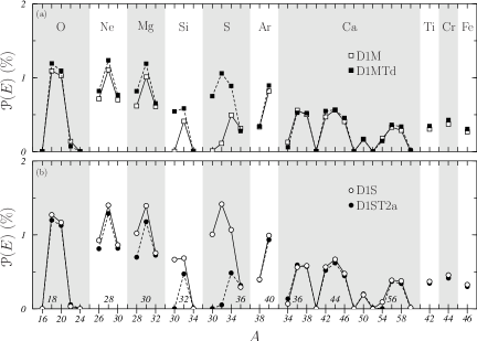
Figure 1: Values of ${\cal P}(E_{\rm HF+BCS,HF})$, defined in Eq. (3), obtained with the four interactions considered, for all the nuclei analyzed.

IV Density distributions

A quantity widely used in the literature to identify SB structures in density distributions is the depletion fraction, which is defined as gra09

$${\cal F}_{\alpha}=\frac{\rho_{\alpha}^{\rm max}-\rho_{\alpha}(0)}{\rho_{\alpha}^{\rm max}}\,.$$ (4)

Here $\rho_{\alpha}^{\rm max}$ is the maximum value reached by $\rho_{\alpha}(r)$, and $\alpha$ stands for proton (p), neutron (n) or matter (m). The density distributions with SB structure have ${\cal F}_{\alpha}>0$.

In Fig. 2 we show the ${\cal F}$ values obtained for proton (squares) and neutron (circles) density distributions for some of the nuclei investigated. The values of ${\cal F}_{\rm n}$ for the Ne, Mg, Si and Ar isotopes and those of ${\cal F}_{\rm p}$ for the Ca nuclei are not shown because they are all zero. We found that the depletion fraction for the matter distribution, ${\cal F}_{\rm m}$, is zero for all the nuclei studied except for the oxygen isotopes with $A<24$ where ${\cal F}_{\rm m}$ is of the same order of ${\cal F}_{\rm p}$ and ${\cal F}_{\rm n}$. In the figure, we compare the results obtained with the D1M (open symbols) and D1S (solid symbols) interactions. The two interactions containing the tensor terms produce ${\cal F}$ values that are not sensitively different from those shown in the figure.

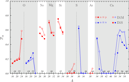
Figure 2: Values of the depletion fraction ${\cal F}$, defined in Eq. (4), for proton (red squares) and neutron (blue circles) density distributions. Open (solid) symbols indicate the results obtained with the D1M (D1S) interaction. Lines are drawn to guide the eyes.

In general, in the nuclei having ${\cal F}_{\rm p}>0$, these are those showing a SB structure in the proton density, the neutron depletion fraction, ${\cal F}_{\rm n}$, is zero and vice-versa. There are, however, two exceptions to this trend. The first one is that of the oxygen isotopes from $A=16$ to 22 in which ${\cal F}_{\rm p}$ and ${\cal F}_{\rm n}$ are both, simultaneously, positive. The second exception concerns the calcium isotopes from $A=40$ to 48 for which ${\cal F}_{\rm p}={\cal F}_{\rm n}=0$.

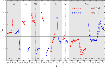
Figure 3: Same as in Fig. 2 for the flatness index ${\cal S}$ defined in Eq. (5).

We investigate the presence of SB structures by using another quantity, the flatness index, that we define as

$${\cal S}_{\alpha}=\frac{\rho_{\alpha}(r_{\rm mean}/2)-\rho_{\alpha}(0)}{\rho_{\alpha}(r_{\rm mean}/2)+\rho_{\alpha}(0)}\,.$$ (5)

In the above expression $r_{\rm mean}$ indicates the root mean squared radius of the density distribution and $\alpha$ has the same meaning as in Eq. (4). An analogous quantity has been used in sch17 . Positive values of ${\cal S}_{\alpha}$ indicate a SB structure in $\rho_{\alpha}$, and if ${\cal S}_{\alpha}<0$ the corresponding density distribution has a maximum at the center of the nucleus. In general, the closer to zero is the value of ${\cal S}_{\alpha}$ the flatter is the density distribution in the nuclear interior.

The values of ${\cal S}_{\rm p}$ and ${\cal S}_{\rm n}$ for the nuclei investigated are shown in Fig. 3. As in the previous figure, squares (circles) indicate the results obtained for the proton (neutron) distributions, and open and solid symbols correspond to D1M and D1S interactions, respectively.

In this figure, the trends already outlined in discussing the ${\cal F}_{\alpha}$ results become more evident: those nuclei having a $\rho_{\rm n}$ with a maximum at the nuclear center, for which ${\cal S}_{\rm n}<0$, show a SB proton density distribution (${\cal S}_{\rm p}<0$) and vice-versa (with the exception of the oxygen isotopes above mentioned). We have found that the sum of the two densities, the matter distribution, is rather flat in all nuclei investigated, with $|{\cal S}_{\rm m}|\sim 0.2$ at most.

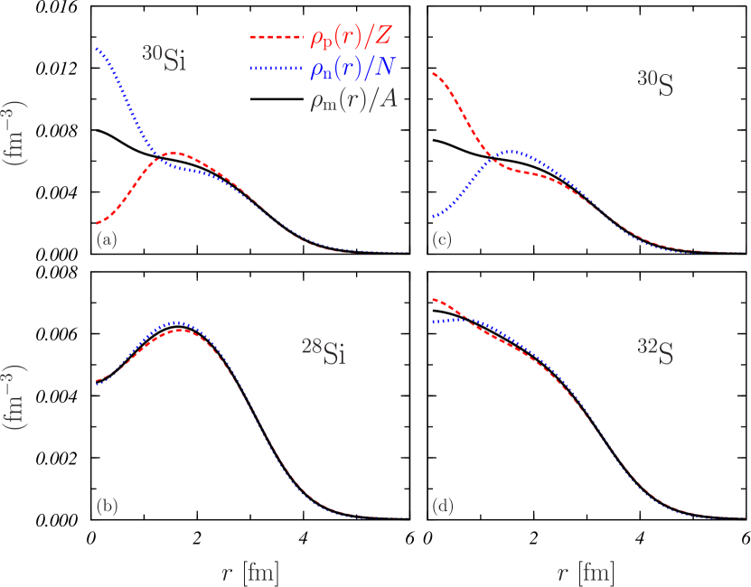
Figure 4: Proton (red dashed lines), neutron (blue dotted lines) and matter (black solid lines) density distributions, normalised to unity, for ²⁸Si, ³⁰Si, ³⁰S and ³²S. The calculations have been carried out with the D1M interaction.

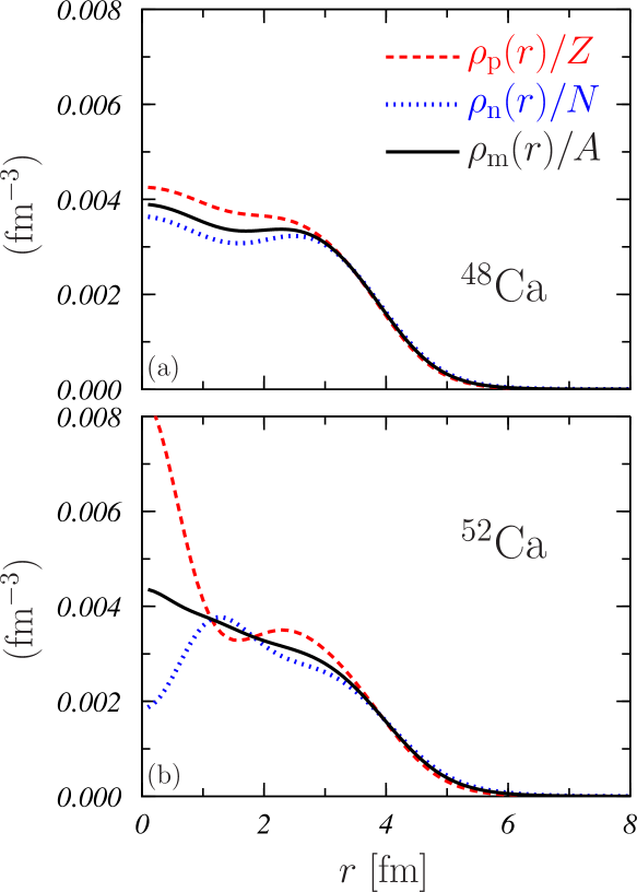
Figure 5: Same as in Fig. 5 but for the ⁴⁸Ca
and ⁵²Ca nuclei.

A clear example of this compensation is provided by the densities of the nuclei in the region around $A=30$. In Fig. 5 we show the proton (red dashed curves), neutron (blue dotted curves) and matter (black full curves) distributions of the ³⁰Si, ³⁰S, ²⁸Si and ³²S nuclei, calculated with the D1M interaction. The densities obtained with the other three interactions are very similar.

The two mirror nuclei ³⁰Si and ³⁰S have high values of ${\cal F}_{\rm p}$ and ${\cal F}_{\rm n}$, respectively. In ³⁰Si, the $2s_{1/2}$ state is empty for protons and full for neutrons; as a consequence, $\rho_{\rm p}$ has a SB behaviour, while $\rho_{\rm n}$ has its maximum at the nuclear center. The opposite occurs in ³⁰S. In both nuclei, the behaviours of $\rho_{\rm p}$ and $\rho_{\rm n}$ counterbalance each other producing matter distributions that do not show SB structures.

Another evidence that the occupancy of the $2s_{1/2}$ s.p. states is the source of the differences between the proton and neutron distributions can be visualized by looking at the densities of ²⁸Si (Fig. 5b) and ³²S (Fig. 5d). Since the ²⁸Si nucleus is deformed, it is not included in the set of the nuclei we have studied. It is, however, interesting to observe that in our spherical HF+BCS description of this nucleus, both the proton and the neutron $2s_{1/2}$ levels are empty, and both $\rho_{\rm p}$ and $\rho_{\rm n}$ have SB structures, and, consequently, also $\rho_{\rm m}$. On the other hand, in ³²S the neutron and proton $2s_{1/2}$ s.p. states have an occupation of 95.7% and 99.9%, respectively. In this case ${\cal F}_{\rm p}=0$ and ${\cal F}_{\rm n}=0.012$ and the corresponding densities do not show SB structures. We can conclude that, in the region of nuclei with $A\sim 30$, the responsible of the appearance of SB structures in proton or neutron density distributions is the occupancy of the $2s_{1/2}$ s.p. levels.

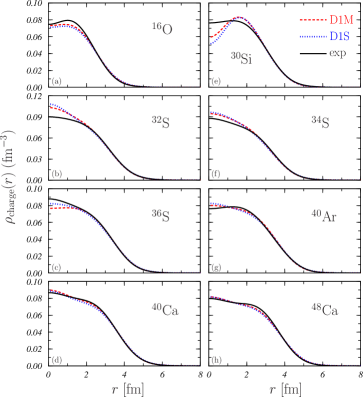
Figure 6: Charge distributions for some of the nuclei studied, calculated with the D1M (red dashed curves) and D1S (blue dotted curves) interactions, compared with the empirical ones (black full curves) taken from the compilation of Ref. dej87 .

The situation is different in $A\sim 50$ region. As example, we show in Fig. 5 the density distributions of the ⁴⁸Ca and ⁵²Ca nuclei obtained with the D1M force. Similar results are found with the other interactions. In these two nuclei both the proton and neutron $2s_{1/2}$ s.p. levels are fully occupied. The proton densities in both nuclei have a maximum at $r=0$, and also $\rho_{\rm n}$ in ⁴⁸Ca, while in ⁵²Ca the neutron distribution show a SB structure. This behavior is due to the filling of the neutron $2p_{3/2}$ s.p. level in ⁵²Ca. The contribution of this state is very small at $r\sim 0$ but it is remarkable at $r\sim 1.5-2\,$fm. In this nucleus, as well as in those in the same mass region, the appearance of a SB structure is due to the filling of s.p. states peaked slightly far from the nuclear center.

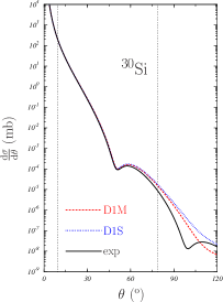
Figure 7: Elastic electron scattering cross sections on ³⁰Si target calculated for an incident electron energy of $300\,$MeV, within the distorted wave Born approximation by using the charge densities shown in panel (b) of Fig. 6. The results obtained with the D1M (red dashed curve) and D1S (blue dotted curve) interactions are compared to those corresponding to the empirical density (black solid curve). The two vertical lines indicate the range probed by the experiment as indicated in Ref. dej87 .

In Fig. 6 we compare the available empirical charge density distributions taken from the compilation of Ref. dej87 with those we have obtained by folding the proton densities with the traditional proton dipole electromagnetic form factor pov93 . The use of more accurate form factors hoe76 produces differences within the numerical accuracy of our calculations. The results obtained with the D1S and D1M interactions are rather similar, especially on the surfaces of the nuclei. The main differences between the various distributions are localized in the nuclear interior.

The empirical charge distributions are obtained by fitting elastic electron scattering data that cover a given range of momentum transfer, $q$, values. By considering that the resolution power is inversely proportional to the maximum momentum transfer involved, the more accurate experiments are those done on ¹⁶O, ⁴⁰Ca and ⁴⁸Ca nuclei where $q_{\rm max}\simeq 3-3.7\,{\rm fm}^{-1}$. The sulfur, ³⁰Si and ⁴⁰Ar data have been taken with $q$ up to $2.6$, 1.5 and $1.8\,$fm^-1, respectively. It is possible that the largest differences observed between our charge densities and the experimental ones, that occur for ³⁰Si (panel (e)) and ³²S (panel (b)) can be fictitious because of the limited resolution power obtained by the experiments.

We illustrate this point by considering the example of the ³⁰Si nucleus. In this case, our calculations predict a remarkable SB structure for both interactions, while the experiment indicates an almost flat density. By using the charge distributions shown in that figure, we have calculated elastic electron scattering cross sections in distorted wave Born approximation. In Fig. 7 we show the results obtained for electrons with an incident energy of $300\,$MeV. The vertical lines indicate the angles corresponding to the smallest and largest momentum transfer probed by the experiment and used to extract the empirical density dej87 . We observe that the differences between empirical and theoretical densities shown in the panel (b) of Fig. 6 generate noticeable effects only at large scattering angles, in a region outside the $q$ range probed by the experiment, indicate by the two vertical lines.

The results of Fig. 6 show that, for all the nuclei considered, the empirical charge densities are well described by our results at the nuclear surface. This is confirmed in Table 4, where the available experimental charge rms radii, taken from the compilation of Ref. ang13 , are compared to those we have obtained with the four interactions considered. The maximum relative deviation from the experimental data is around $3\%$. This good agreement is not surprising since charge rms radii were inserted in the fit procedure to determine the values of the parameters of the D1S and D1M interactions cha07t .

element	$A$	D1M	D1S	D1MTd	D1ST2a	exp		element	$A$	D1M	D1S	D1MTd	D1ST2a	exp
O	16	$2.76$	$2.79$	$2.76$	$2.79$	$2.70$		Ar	38	$3.39$	$3.42$	$3.39$	$3.43$	$3.40$
	18	$2.77$	$2.80$	$2.77$	$2.80$	$2.77$			40	$3.39$	$3.43$	$3.39$	$3.43$	$3.43$
	20	$2.78$	$2.81$	$2.78$	$2.81$	—		Ca	34	$3.47$	$3.51$	$3.46$	$3.50$	—
	22	$2.80$	$2.82$	$2.79$	$2.82$	—			36	$3.47$	$3.49$	$3.46$	$3.49$	—
	24	$2.80$	$2.83$	$2.79$	$2.83$	—			38	$3.46$	$3.49$	$3.46$	$3.49$	—
Ne	26	$2.91$	$2.95$	$2.92$	$2.97$	$2.93$			40	$3.46$	$3.50$	$3.46$	$3.50$	$3.48$
	28	$2.97$	$3.01$	$2.97$	$3.02$	$2.96$			42	$3.48$	$3.51$	$3.47$	$3.51$	$3.51$
	30	$3.03$	$3.07$	$3.03$	$3.07$	—			44	$3.49$	$3.52$	$3.49$	$3.52$	$3.52$
Mg	28	$2.99$	$3.02$	$3.00$	$3.06$	—			46	$3.50$	$3.52$	$3.49$	$3.52$	$3.50$
	30	$3.06$	$3.10$	$3.07$	$3.11$	—			48	$3.50$	$3.53$	$3.50$	$3.53$	$3.48$
	32	$3.11$	$3.15$	$3.11$	$3.16$	—			50	$3.56$	$3.57$	$3.56$	$3.57$	$3.52$
Si	30	$3.06$	$3.08$	$3.08$	$3.12$	$3.13$			52	$3.62$	$3.62$	$3.67$	$3.62$	—
	32	$3.12$	$3.15$	$3.13$	$3.17$	—			54	$3.72$	$3.72$	$3.71$	$3.72$	—
	34	$3.18$	$3.21$	$3.18$	$3.21$	—			56	$3.72$	$3.73$	$3.72$	$3.73$	—
S	30	$3.25$	$3.26$	$3.26$	$3.29$	—			58	$3.74$	$3.75$	$3.74$	$3.75$	—
	32	$3.24$	$3.27$	$3.26$	$3.30$	$3.26$			60	$3.77$	$3.77$	$3.75$	$3.77$	—
	34	$3.27$	$3.29$	$3.28$	$3.31$	$3.29$		Ti	42	$3.55$	$3.59$	$3.55$	$3.59$	—
	36	$3.29$	$3.33$	$3.29$	$3.33$	$3.30$		Cr	44	$3.62$	$3.66$	$3.61$	$3.66$	—
								Fe	46	$3.67$	$3.72$	$3.67$	$3.72$	—

Table 4: Charge root mean square radii, in fm, calculated in HF+BCS approach, for all the nuclei considered, with the four interactions used in this work. The experimental values are taken from Ref. ang13 .

We conclude this section briefly discussing the role of the pairing on the density distributions. In general, the effect of the pairing on this observable is negligible. There are, however, some remarkable exceptions to this general trend. The pairing reduces the ${\cal F}$ values for the neutron distributions of ²⁰O and ²²O of about the 10%. We found larger effects on the ${\cal F}$ values of the proton distributions of ³⁶S and ⁴⁰Ar and those of the neutron distributions of ³⁶Ca and ³⁸Ca which are almost doubled by the inclusion of the pairing.

V Spin-orbit splitting

We have pointed out in the previous section that the experimental investigation of the presence of a SB structure in the proton, or charge, density distribution requires a high spatial resolution, therefore elastic electron scattering experiments involving high values of the momentum transfer. However, these experiments are rather difficult to carry out, especially on unstable nuclei. In the following we address the question whether there are subsidiary observables that can be related to the occurrence of SB structures in nuclear densities.

According to Ref. vau72 , the contribution of the s.o. term of the interaction to the total energy of the system is given by

$$E_{\rm s.o.}\,=\,\frac{1}{2}\,W_{0}\int{\rm d}^{3}r\,(\nabla\rho_{\rm m}\cdot{\bf J_{\rm m}}\,+\,\nabla\rho_{\rm n}\cdot{\bf J}_{\rm n}\,+\,\nabla\rho_{\rm p}\cdot{\bf J}_{\rm p})\,,$$ (6)

where the spin density ${\bf J}_{\tau}$ is defined as

$${\bf J}_{\tau}({\bf r})\,=\,-\,i\,\sum_{\alpha\sigma\sigma^{\prime}}[\phi^{\tau}_{\alpha\sigma}({\bf r})]^{*}\,\left[\nabla\phi^{\tau}_{\alpha\sigma^{\prime}}({\bf r})\times\langle\sigma|\mbox{\boldmath$\sigma$}|\sigma^{\prime}\rangle\right]\,,\,\,\,\,\,\tau\equiv{\rm p},{\rm n}\,,$$ (7)

and ${\bf J}_{\rm m}={\bf J}_{\rm p}+{\bf J}_{\rm n}$. In the above equations $\phi$ indicates the s.p. wave function characterized by the third components of the isospin, $\tau$, and of the spin, $\sigma$, and by other quantum numbers $\alpha$.

As we can see in Eq. (6), the value of $E_{\rm s.o.}$ depends on the derivative of the density distributions. Therefore, the presence of a SB structure could show up in the s.o. energy because it would make $\nabla\rho$ to behave in the nuclear interior with opposite sign with respect to the surface, thus producing an overall reduction. We investigate if some observable linked to the s.o. interaction can be used to reveal SB structure in nuclei. The relationship between the s.o. interaction and the SB structure in density distribution has been investigated in Refs. gra09 ; wan11 ; li16 ; dug17 ; bur11t ; bur14 ; mut15t ; shu16 ; mut17 ; kar17 ; tod04 ; wu14 .

We have estimated the order of magnitude of the effect described above by performing a toy calculation for the ⁴⁰Ca nucleus. First, we have obtained two sets of s.p. wave functions from a mean-field potential of the form

$$V(r)\,=\,\frac{V_{0}}{1\,+\,\exp\left(\displaystyle\frac{r\,-\,R}{a}\right)}\,+\,B\,\exp\left(-\displaystyle\frac{r^{2}}{b^{2}}\right)\,.$$ (8)

The second term of the above equation has been used to generate density profiles with SB structure.

The values $V_{0}=-50\,$MeV, $R=4.4\,$fm, $a=0.6\,$fm, and $b=0.5\,$fm have been chosen for both protons and neutrons. We have considered $B=0$ and $B=140\,$MeV to obtain the proton s.p. wave function of the two sets; for the neutron ones we used $B=0$ in the two cases. Using these s.p. wave functions, the direct Hartree, $\Gamma_{\rm d}({\bf r})$, and the exchange Fock-Dirac, $\Gamma_{\rm ex}({\bf r},{\bf r}^{\prime})$, potentials rin80 entering into the HF equations have been calculated for the D1M interaction and then we have solved the one-body Schrödinger equation

$$-\frac{\hbar^{2}}{2m}\nabla^{2}\phi_{k}({\bf r})\,+\,\Gamma_{\rm d}({\bf r})\,\phi_{k}({\bf r})\,-\,\int{\rm d}{\bf r}^{\prime}\,\Gamma_{\rm ex}({\bf r},{\bf r}^{\prime})\,\phi_{k}({\bf r}^{\prime})\,=\,\epsilon_{k}\,\phi_{k}({\bf r})$$ (9)

to obtain the corresponding s.p. states as well as their energies.

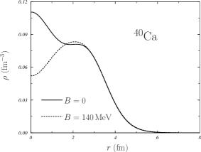
Figure 8: Proton distribution for the ⁴⁰Ca nucleus obtained by using the mean-field potential of Eq. (8). The full line has been obtained without the gaussian term, $B=0$, in Eq. (8). The dashed line is the result obtained by inserting the gaussian term with the parameters indicated in the text.

We show in Fig. 8 the proton density distributions corresponding to the full potential (dashed curve) and to the potential with $B=0$ (solid curve). The former has a SB structure with ${\cal F}_{\rm p}=0.37$. From the solutions of Eq. (9) we have evaluated the s.o. splitting

$$s^{\alpha}_{nl}\,=\,\epsilon_{nlj-1/2}\,-\,\epsilon_{nlj+1/2}\,,\,\,\,\,\alpha\equiv{\rm p,n}\,,$$ (10)

where $\epsilon$ labels the s.p. energy and $n$, $l$ and $j$ are the quantum numbers characterizing the state. In the calculation with $B=0$, i.e. without SB structure, we have found that $s^{\rm p}_{1p}=3.24\,$MeV and $s^{\rm p}_{1d}=4.84\,$MeV. These values reduce to $0.53\,$MeV and $3.40\,$MeV when the densities with SB structure are used.

Once the order of magnitude of the expected effect, given by the reduction of the $s_{nl}$ values just discussed, was evaluated, we analysed the s.o. splittings obtained in our HF+BCS calculations for all the nuclei we are studying. In Fig. 9 we show the neutron splittings $s^{\rm n}_{2p}$ (panel (a)), $s^{\rm n}_{1d}$ (panel (b)) and $s^{\rm n}_{1p}$ (panel (c)) as a function of $A$ for the Si, S, and Ca isotope chains. Green squares, blue triangles, red circles and black diamonds indicate the values calculated with the D1M, D1S, D1MTd and D1ST2a interactions, respectively.

The only recurring effect we observe is an increase of the splitting when going from $N=14$ to $N=16$; these values of $N$ are represented by vertical dotted lines in the figure. This behavior is related to the filling of the neutron $2s_{1/2}$ level. In the case of $N=14$ this level is empty and this generates a SB neutron distribution, as can be checked in Figs. 2 and 3. All the nuclei with $N=16$ have the neutron $2s_{1/2}$ level fully occupied and the corresponding neutron densities do not show SB structure.

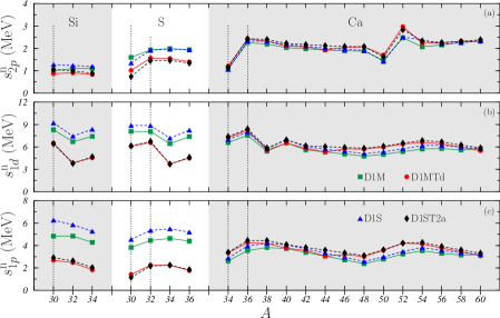
Figure 9: HF+BCS spin orbit splitting $s_{nl}$, defined in Eq. (10), for neutron $1p$, $1d$ and $2p$ s.p. states. The results obtained for the Si, S, Ar and Ca isotope chains are shown as a function of $A$. Green squares, blue triangles, red circles and black diamonds indicate the values calculated with the D1M, D1S, D1MTd and D1ST2a interactions, respectively. The vertical dotted lines indicate the nuclei with $N=14$ and $N=16$.

A similar increase in the splitting is observed between $N=30$ and $N=32$ in Ca, for the $2p$ level only, and between $N=18$ and $N=20$ for the $1d$ state in the three isotope chains. In these cases, the effect is linked to the fact that the neutron $2p_{3/2}$ and $1d_{3/2}$ states are fully occupied for $N=32$ and $N=20$, respectively. However, while in the first case, the Ca involved present a SB structure in the neutron density, with a ${\cal S}_{\rm n}$ value that increases with the splitting, none of the nuclei with $N=18$ and $N=20$ show SB neutron densities (see Figs. 2 and 3).

We observe an analogous behaviour in Fig. 10 where we show, as a function of $A$, the values of $s^{\rm p}_{nl}$ for the $2p$ (panel (a)), $1d$ (panel (b)) and $1p$ (panel (c)) proton s.p. states and for the isotone chains with $N=16$, 18, and 20. Again, $s_{nl}$ increases between $Z=14$ and $Z=16$ (indicated with the dotted vertical lines in the figure), the nuclei with $Z=14$ having SB proton densities, while those with $Z=16$ do not. This behaviour is related to the occupation of the proton $2s_{1/2}$ s.p. level. However, some exceptions occur in $N=16$: $s^{\rm p}_{2p}$, for D1M, D1S and D1MTd, and $s^{\rm p}_{1d}$, for D1M and D1S. As in the case of Fig. 9, we observe a systematic increase of the $s_{1d}$ values from $Z=18$ to $Z=20$ in all the interactions for $N=20$.

Both Figs. 9 and 10 show that the increase of the $s_{nl}$ values when the number of proton or neutrons changes from 14 to 16 occurs for the four interactions considered, independently of the inclusion of tensor terms. This is important since the s.o. splittings may be strongly influenced by these terms ots06 , as it can be seen for $1d$ and $1p$ s.p. levels in Si and S (Fig. 9) and in $N=16$ (Fig. 10). In these cases the results obtained with the interactions containing tensor terms are about 2 MeV smaller than those obtained with the D1M and D1S forces. This is a consequence of the effect described by Otsuka ots06 that predicts a reduction of the splitting between the energies of the s.o. partner levels due to the contribution of the unlike particle term of the tensor force. This effect becomes smaller in nuclei with proton or neutron s.o. saturated levels.

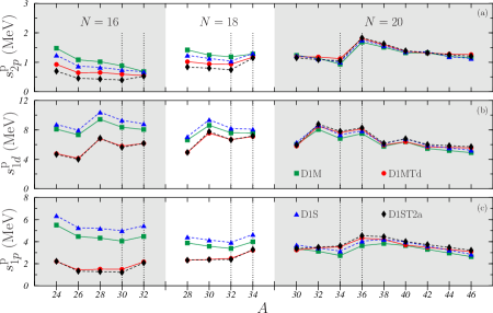
Figure 10: HF+BCS spin orbit splitting $s_{nl}$, as defined in Eq. (10), for proton $1p$, $1d$ and $2p$ s.p. states. The results obtained for the $N=16$, 18, 20 and 22 isotone chains are shown as a function of $A$. Green squares, blue triangles, red circles and black diamonds indicate the values calculated with the D1M, D1S, D1MTd and D1ST2a interactions, respectively. The vertical dotted lines indicate the nuclei with $Z=14$ and $Z=16$.

In Refs. bur11t ; mut15t it is reported that the s.o. splitting $s_{2p}^{\rm p}$ of ³⁶S is larger than that of ³⁴Si. This is in agreement with the results of our calculations.

VI Excitation spectra

The instability of the nuclei where we have identified the presence of SB structures generates an intrinsic difficulty in using them as targets of scattering experiments. On the other hand, the study of the excitation spectra is a, relatively, easier task. For this reason, after having verified that a SB density distribution is linked to the size of the splitting between the energies of the s.o. partner levels, we analyzed how this influences the excitation spectra.

$J^{\pi}$	nucleus	D1M	D1S	D1MTd	D1ST2a	exp
$2^{+}$	34Si	3.99	4.30	4.00	4.25	3.33
	36S	1.81	2.03	1.56	1.62	3.30
$3^{+}$	34Si	4.74	5.70	4.00	4.91	—
	36S	7.68	8.20	7.63	8.10	5.46
$4^{+}$	34Si	6.77	6.78	6.64	6.42	—
	36S	7.15	7.12	7.09	6.83	6.51
$1^{+}$	34Si	8.12	9.12	5.00	7.46	—
	36S	8.47	9.37	8.40	8.38	4.52
$2^{+}$	34Ca	3.55	3.88	3.86	3.85	—
	36Ca	2.51	2.72	2.39	2.49	—
$3^{+}$	34Ca	4.68	5.58	4.70	4.70	—
	36Ca	8.14	8.48	8.51	8.59	—
$4^{+}$	34Ca	6.73	6.73	6.72	6.31	—
	36Ca	7.55	7.31	7.33	7.13	—
$1^{+}$	34Ca	8.15	9.13	7.72	7.44	—
	36Ca	9.01	9.78	8.74	8.77	—

Table 5: Excitation energies, expressed in MeV, of ³⁴Si, ³⁶S, ³⁴Ca and ³⁶Ca nuclei. The experimental data are from Ref. bnlw .

We investigated excited states dominated by particle-hole configurations involving s.o. partner levels. This implies the study of positive parity states, $0^{+}$ excitations excluded. We have carried out our calculations by using the QRPA approach described in detail in Ref. don17 .

We present, in Table 5, the results obtained for the $N=20$ isotones ³⁴Si and ³⁶S and for the $Z=20$ isotopes ³⁴Ca and ³⁶Ca. In these nuclei the shell closure at 20 induces low-lying excitations dominated by the protons in ³⁴Si and ³⁶S and by the neutrons in the calcium isotopes. We have selected these nuclei since the open shells are filled by 14 or 16 nucleons where we found the main effect of the SB structure on the s.p. energies.

In Table 5 we show the excitation energies for the positive parity states obtained with the four interactions we have considered, and we compare them with available experimental data, taken from the compilation of Ref. bnlw . We observe that the differences between the energies obtained with the four interactions are 1.5 MeV at most, with the exception of the $1^{+}$ state in ³⁴Si that shows a rather small excitation energy in the case of the D1MTd force. In this case, the tensor terms generate high collectivity in the wave function that is not present when the other interactions are considered.

Remarkable discrepancies with the available experimental data are those of the $2^{+}$ state in ³⁶S, which is underestimated by more than $1.5\,$MeV, and the $1^{+}$ and $3^{+}$ states in the same nucleus, overestimated by about $4\,$MeV and $2\,$MeV, respectively. In the $4^{+}$ case the differences between our results and the experimental data are about $1\,$MeV.

When going from ³⁴Si to ³⁶S and from ³⁴Ca to ³⁶Ca, the energy of the $2^{+}$ state diminishes of about $2\,$MeV and $1.5\,$MeV, respectively. For the other excited states analyzed, the energies increase, specially for the $3^{+}$ states. We have to remark, however, that the $3^{+}$ states in the nuclei with $A=34$ are dominated by the $(2s_{1/2},1d_{5/2})$ configuration while for $A=36$ the main configuration is $(1d_{3/2},1d_{5/2})$. As a consequence a direct relation between the change in the s.o. splitting and the variation in the excitation energy cannot be established. A similar situation occurs for the $2^{+}$ excited states.

$4^{+}$
	$\omega$	$(1d_{3/2},1d_{5/2})_{\rm p}$			$(1d_{3/2},1d_{5/2})_{\rm n}$				$\omega$	$(1d_{3/2},1d_{5/2})_{\rm p}$			$(1d_{3/2},1d_{5/2})_{\rm n}$
nucleus	(MeV)	$|X|$	$|Y|$		$|X|$	$|Y|$		nucleus	(MeV)	$|X|$	$|Y|$		$|X|$	$|Y|$
30Si	6.32	0.74	0.09		0.67	0.09		32S	5.90	0.73	0.10		0.68	0.10
32Si	6.54	0.84	0.07		0.52	0.05		34S	6.41	0.82	0.07		0.55	0.06
34Si	6.77	0.99	0.05		—	—		36S	7.15	0.99	0.03		—	—
30S	6.96	0.74	0.08		0.66	0.08		32S	5.90	0.73	0.10		0.68	0.10
34Ca	6.73	—	—		0.99	0.05		36Ca	7.55	—	—		0.99	0.03

Table 6: Excitation energies of the $4^{+}$ states in various silicon, sulfur, argon and calcium isotopes and QRPA amplitudes of the main configurations of the corresponding wave functions, obtained by using the D1M interaction.

	D1M	D1S	D1MTd	D1ST2a
$s^{\rm p}_{1d}(^{36}{\rm S})-s^{\rm p}_{1d}(^{34}{\rm Si})$ (MeV)	0.62	1.41	0.50	0.51
$\omega_{4^{+}}(^{36}{\rm S})-\omega_{4^{+}}(^{34}{\rm Si})$ (MeV)	0.38	0.34	0.45	0.41
${\cal F}_{\rm p}(^{36}{\rm S})-{\cal F}_{\rm p}(^{34}{\rm Si})$	$-0.24$	$-0.49$	$-0.30$	$-0.51$
${\cal S}_{\rm p}(^{36}{\rm S})-{\cal S}_{\rm p}(^{34}{\rm Si})$	$-0.24$	$-0.36$	$-0.24$	$-0.38$
$s^{\rm n}_{1d}(^{36}{\rm Ca})-s^{\rm n}_{1d}(^{34}{\rm Ca})$ (MeV)	1.10	1.02	0.78	1.06
$\omega_{4^{+}}(^{36}{\rm Ca})-\omega_{4^{+}}(^{34}{\rm Ca})$ (MeV)	0.81	0.59	0.62	0.82
${\cal F}_{\rm n}(^{36}{\rm Ca})-{\cal F}_{\rm n}(^{34}{\rm Ca})$	$-0.17$	$-0.31$	$-0.23$	$-0.29$
${\cal S}_{\rm n}(^{36}{\rm Ca})-{\cal S}_{\rm n}(^{34}{\rm Ca})$	$-0.13$	$-0.23$	$-0.17$	$-0.23$

Table 7: Differences between various quantities calculated in the two pairs of nuclei ³⁶S$-^{34}$Si and ³⁶Ca$-^{34}$Ca. Specifically, the differences between (i) the s.p. energies of the proton or neutron $d$ levels; (ii) the QRPA energies of the $4^{+}$ excitations; (iii) the values of the depletion fraction ${\cal F}$, defined in Eq. (4), and (iv) those of the flatness index ${\cal S}$, defined in Eq. (5) are given..

To avoid this problem we have focussed our attention on $4^{+}$ excitations that are rather well selective for the configurations involving the $1d$ s.o. partner levels. We summarize in Table 6 the results obtained for various isotopes grouped in pairs that have the same number of either neutrons or protons and, simultaneously have either $Z=14,16$ or $N=14,16$. We include only the results obtained with the D1M interaction, those found for the other forces being similar. In all the cases, the dominant p-h configurations are the proton $(1d_{3/2},1d_{5/2})_{\rm p}$ and the neutron $(1d_{3/2},1d_{5/2})_{\rm n}$. Specifically, we show the energies of the $4^{+}$ excited states and the absolute values of the QRPA amplitudes $X$ and $Y$ don17 when $|X|>0.1$.

We observe that only in the ³⁴Si and ³⁶S nuclei the excitation is dominated by a single proton $(1d_{3/2},1d_{5/2})_{\rm p}$ configuration. In a similar way, only in the case of the ³⁴Ca and ³⁶Ca the excited state is an almost pure neutron $(1d_{3/2},1d_{5/2})_{\rm n}$ configuration. In the other nuclei, the opening of both neutron and proton shells allows a mixture of the $(1d_{3/2},1d_{5/2})_{\rm p}$ and $(1d_{3/2},1d_{5/2})_{\rm n}$ components in the wave functions. In these latter nuclei, the excitation energy is a kind of average of the energies of these two configurations.

In Table 7 we compare, for the four interactions, the results obtained for various quantities related to the SB structure of the density. For the two pairs of nuclei (³⁶S$-^{34}$Si and ³⁶Ca$-^{34}$Ca), we have evaluated the differences between the respective s.o. splittings $s_{1d}^{\alpha}$, excitation energies of the $4^{+}$ states, $\omega_{4^{+}}$, depletion fraction ${\cal F}_{\alpha}$ and flatness index ${\cal S}_{\alpha}$. As we can see, a reduction in ${\cal F}$, and in ${\cal S}$, occurs when going from $A=34$ to $A=36$, indicating that the corresponding density looses its SB structure, as it is clearly shown in Fig. 11. This is related to an increase of the excitation energy of the $4^{+}$ state due to an enhancement in the s.o. splitting of the $1d$ s.p. level. This happens for the two pairs of nuclei and for all the interactions.

From what we have discussed the identification of $4^{+}$ states in the spectra of the four nuclei considered can be used to infer the presence of a SB structure in the $A=34$ nuclei. As it is shown in Table 5 only the $4^{+}$ state in ³⁶S has been identified at about $6.51\,$MeV. By considering the range of uncertainty of our calculations, related to the use of different nucleon-nucleon interactions, we would expect a $4^{+}$ state in ³⁴Si between 6.0 and $6.2\,$MeV. The state identified at $6.023\,$MeV and whose multipolarity has not yet been assigned bnlw could be that $4^{+}$ level.

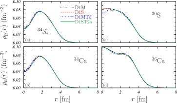
Figure 11: Density distributions of protons, panels (a) and (c), and neutrons, panels (b) and (d), of the nuclei analyzed in Table 7. The four lines indicate the results obtained by using the four interactions considered in the present work.

VII Conclusions

In this article we have investigated the possibility that some nuclei present a SB structure in their proton, neutron or matter distributions. Since a direct identification of these structures requires very involved scattering experiments difficult to be carry out on unstable targets, we have explored the possibility that the SB distributions can be linked to observables more easily measurables. The relationship between the derivative of the distributions and the s.o. interaction induced us to study the energy splittings of s.o. partner levels, and also the energy spectra.

In our investigation we used a HF+BCS approach that generates the s.p. bases required as input for our QRPA calculations of the excited states. These calculations have been done for spherical nuclei, by using the same interaction in all the three steps, HF, BCS and QRPA. We used four different parameterizations of the finite-range Gogny force, two of them containing tensor terms. In this way we have estimated the sensitivity of our results to the only physical input of our approach: the effective nucleon-nucleon interaction.

The validity of our calculations has been tested against the experimental binding energies, and we found excellent agreements. Also the experimental values of the charge rms radii are rather well reproduced. We have compared the charge distributions obtained in our calculations with the available empirical ones. While their behaviors are well reproduced on the nuclear surface, there are some discrepancies in the interior, where the SB structures appear.

However, since investigating the nuclear interior is rather difficult we have studied the effects of the SB structures on other observables such as those linked to the s.o. interaction. We have pragmatically verified that there is a relationship between the occurrence of SB structures in the density distributions and the size of the splitting between the energies of s.p. levels that are s.o. partners. The general trend we found is that the s.o. splittings in isotones, or isotopes, with 14 protons, or neutrons, that have SB structures in their proton, or neutron densities, are smaller than those with 16, where SB distributions do not occur. The differences are relatively large and this behaviour occurs in all the calculations we have carried out, independently of the interaction used and all along the various isotope and isotone chains studied.

This modification of the s.o. energy splitting has consequences on the excitation spectrum. We have studied with our QRPA theory the positive parity excited states of various nuclei. We have found that the most interesting cases are the low-lying $4^{+}$ states in the isotones ³⁴Si and ³⁶S, and in the isotopes ³⁴Ca and ³⁶Ca. In these nuclei, the $4^{+}$ excitation is dominated by a single, almost pure configuration formed by the $1d$ s.o. partners levels. We have found that the $4^{+}$ excited states in $A=34$ nuclei have lower energies than the analogous ones in the $A=36$ nuclei.

At present only a $4^{+}$ state in ³⁶S at $6.5\,$MeV is known. Our calculations predict a $4^{+}$ state in ³⁴Si at about 6.0 MeV. The identification of this state would validate our approach and indicate the existence of a SB structure in ³⁴Si.

- (1) C. Y. Wong, Phys. Lett. B 41 (1972) 451.
- (2) J. Dechargé, J.-F. Berger, M. Girod, K. Dietrich, Nucl. Phys. A 716 (2003) 55.
- (3) K. Davies, C. Y. Wong, S. Krieger, Phys. Lett. B 41 (1972) 455.
- (4) X. Campi, D. Sprung, Phys. Lett. B 46 (1973) 291.
- (5) J. Friedrich, N. Voegler, P. G. Reinhard, Nucl. Phys. A 459 (1986) 10.
- (6) E. Khan, M. Grasso, J. Margueron, N. Van Giai, Nucl. Phys. A 800 (2008) 37.
- (7) M. Grasso, L. Gaudefroy, E. Khan, T. Nikšić, J. Piekarewick, O. Sorlin, N. V. Giai, D. Vretenar, Phys. Rev. C 79 (2009) 034318.
- (8) Y. Chu, Z. Ren, Z. Wang, T. Dong, Phys. Rev. C 82 (2010) 024320.
- (9) Y. Z. Wang, J. Z. Gu, X. Z. Zhang, J. M. Dong, Phys. Rev. C 84 (2011) 044333.
- (10) J.-M.Yao, S. Baroni, M. Bender, P.-H. Heenen, Phys. Rev. C 86 (2012) 014310.
- (11) A. Meucci, M. Vorabbi, C. Giusti, F. D. Pacati, P. Finelli, Phys. Rev. C 89 (2014) 034604.
- (12) J. J. Li, W. H. Long, J. L. Song, Q. Zhao, Phys. Rev. C 93 (2016) 054312.
- (13) T. Duguet, V. Somà, S. Lecluse, C. Barbieri, P. Navrátil, Phys. Rev. C 95 (2017) 034319.
- (14) B. Schuetrumpf, W. Nazarewicz, P.-G. Reinhard, Phys. Rev. C 96 (2017) 024306.
- (15) S. Boffi, C. Giusti, F. D. Pacati, M. Radici, Electromagnetic response of atomic nuclei, Clarendon, Oxford, 1996.
- (16) H. Simon, Nucl. Phys.a 787 (2007) 102.
- (17) T. Suda, et al., Phys. Rev. Lett. 102 (2009) 102501.
- (18) G. Burgunder, Étude de l’interaction nucléaire spin-orbite par réaction de transfert 36S S et 34S S., Ph.D. thesis, Université de Caen (France), http://tel.archives-ouvertes.fr/tel-00595010 (2011).
- (19) G. Burgunder, at el., Phys. Rev. Lett. 112 (2014) 042502.
- (20) A. Mutschler, Le noyau-bulle de 34Si: Un outil expérimental pour étudier l’interaction spin-orbite?, Ph.D. thesis, Université de Paris Sud - Paris XI (France), http://tel.archives-ouvertes.fr/tel-01206188 (2011).
- (21) A. Mutschler, et al., Nature Phys. 13 (2017) 152.
- (22) M. Anguiano, A. M. Lallena, G. Co’, V. De Donno, J. Phys. G 41 (2014) 025102.
- (23) V. De Donno, G. Co’, M. Anguiano, A. M. Lallena, Phys. Rev. C 95 (2017) 054329.
- (24) M. Anguiano, A. M. Lallena, G. Co’, V. De Donno, J. Phys. G 42 (2015) 079501.
- (25) M. Anguiano, R. N. Bernard, A. M. Lallena, G. Co’, V. De Donno, Nucl. Phys. A 955 (2016) 181.
- (26) J. F. Berger, M. Girod, D. Gogny, Comp. Phys. Commun. 63 (1991) 365.
- (27) F. Chappert, M. Girod, S. Hilaire, Phys. Lett. B 668 (2008) 420.
- (28) F. Chappert, Nouvelles paramétrisation de l’interaction nucléaire effective de Gogny, Ph.D. thesis, Université de Paris-Sud XI (France), http://tel.archives-ouvertes.fr/tel-001777379/en/ (2007).
- (29) S. Goriely, S. Hilaire, M. Girod, S. Péru, Phys. Rev. Lett. 102 (2009) 242501.
- (30) M. Anguiano, M. Grasso, G. Co’, V. De Donno, A. M. Lallena, Phys. Rev. C 86 (2012) 054302.
- (31) M. Grassso, M. Anguiano, Phys. Rev. C 88 (2013) 054328.
- (32) J. M. Blatt, V. F. Weisskopf, Theoretical nuclear physics, John Wiley and sons, New York, 1952.
- (33) M. Anguiano, G. Co , V. De Donno, A. M. Lallena, Phys. Rev. C 83 (2011) 064306.
- (34) T. Otsuka, T. Matsuo, D. Abe, Phys. Rev. Lett. 97 (2006) 162501.
- (35) S. Hilare, M. Girod, CEA, http://www-phynu.cea.fr/science_en_ligne/carte_potentiels_microscopiques/carte_potentiel_nucleaire.htm.
- (36) M. Anguiano, J. L. Egido, L. M. Robledo, Nucl. Phys. A 683 (2001) 227.
- (37) Brookhaven National Laboratory, National nuclear data center, http://www.nndc.bnl.gov/.
- (38) C. W. De Jager, C. De Vries, At. Data Nucl. Data Tables 36 (1987) 495.
- (39) B. Povh, K. Rith, C. Scholz, F. Zetche, Teilchen und Kerne: Eine Einfürung in die physicalischen Konzepte, Springer, Berlin, 1993.
- (40) G. Hoeler, E. Pietarinen, I. Sabba-Stefanescu, F. Borkowski, G. G. Simon, V. H. Walther, R. D. Wendling, Nucl. Phys. B 114 (1976) 505.
- (41) I. Angeli, K. P. Marinova, Atomic Data and Nuclear Data Tables 99 (2013) 69.
- (42) D. Vautherin, D. M. Brink, Phys. Rev. C 5 (1972) 626.
- (43) A. Shukla, S. Åberg, A. Bajpeyi, Phys. Atom. Nucl. 79 (2016) 11.
- (44) K. Karakatsanis, G. A. Lalazissis, P. Ring, E. Litvinova, Phys. Rev. C 95 (2017) 034318.
- (45) B. G. Todd-Rutel, J. Piekarewicz, P. D. Cottle, Phys. Rev. C 69 (2004) 021301(R).
- (46) X. Y. Wu, J. M. Yao, Z. P. Li, Phys. Rev. C 89 (2014) 017304.
- (47) P. Ring, P. Schuck, The nuclear many-body problem, Springer, Berlin, 1980.