A slip-based model for the size-dependent effective thermal conductivity of nanowires

Abstract

The heat flux across a nanowire is computed based on the Guyer-Krumhansl equation. Slip conditions with a slip length depending on both temperature and nanowire radius are introduced at the outer boundary. An explicit expression for the effective thermal conductivity is derived and compared to existing models across a given temperature range, providing excellent agreement with experimental data for Si nanowires.

Keywords: Heat Transfer, Nanotechnology, Thermal Conductivity, Guyer-Krumhansl, Phonon Hydrodynamics

1 Introduction

Nanotechnology is currently the focus of extensive research due to its wide range of applications in fields such as industry and medicine [1, 2, 3, 4, 5, 6, 7]. Nanowires, in particular, are being used in technologies relating to solar cells [4], flexible screens [5], detection of cancerous cells [7], and energy storage [6]. A key issue facing the practical use of nanodevices is thermal management [8]. Inefficient regulation of heat can lead to large temperatures and melting, possibly resulting in device failure. Understanding and predicting heat flow on the nanoscale is therefore crucial for the manufacturing and operation of nanotechnologies.

It is widely known that many thermophysical material properties become size-dependent at the nanoscale [9, 10, 11, 12, 13, 14, 15, 16]. Buffat and Borel [9] showed a dramatic decrease of the melting temperature of gold nanoparticles of almost 50% from the bulk value. For aluminium nanoparticles, a decrease in latent heat by a factor of four has been reported [10]. Experimental observations also demonstrate that the thermal conductivity in silicon nanowires is much lower than the theoretical value predicted by kinetic theory [14]. For instance, it is reported that, at room temperature, the thermal conductivity of Si nanowires with a diameter of 37 nm decreases by approximately 87% with respect to the bulk value. Furthermore, when the characteristic size of the system is much smaller than the phonon mean free path, the thermal conductivity shows an approximately linear dependence on size [17, 18, 19, 20].

The size dependence of the thermal conductivity of nanosystems is attributed to the fact that, on the nanoscale, the transport of thermal energy is a ballistic process driven by infrequent collisions between thermal energy carriers known as phonons. This is in contrast to macroscopic heat transfer, which is a diffusive processes driven by frequent phonon collisions. As the size of a device becomes commensurate with the phonon mean free path, bulk phonons are more likely to collide with a boundary than with each other. The ability of a nanodevice to conduct thermal energy, therefore, becomes strongly influenced by the scattering dynamics at the boundary as well as the geometrical structure (e.g., size and shape) of this boundary.

Due to the fundamentally different manner in which heat is transported across nanometer length scales in comparison to heat flow at the macroscale, Fourier’s law is unable to provide an accurate description of heat conduction in this regime [21]. Different approaches to modelling nanoscale heat flow have been developed in order to capture the ballistic nature of energy transport and size dependence of the effective thermal conductivity (ETC). These approaches can be classified into three main categories: microscopic, mesoscopic and macroscopic models. Microscopic approaches, such as molecular dynamics or Monte-Carlo methods [22], focus on the evolution of every single phonon while mesoscopic models group them together depending on their wavelength and wavevector. Micro and mesoscopic models are mainly based on the Boltzmann transport equation (BTE) and its solution under different approximations. A popular example is the equation of phonon radiative transfer (EPRT) [23], where an expression for the ETC similar to the classical expression from kinetic theory is derived, although here an effective mean free path is now considered. However this model is based on the gray approximation and thus considers a single phonon group velocity and lifetime. A more general model where these quantities are mode-dependent was presented by McGaughey et al. [24]. Starting again from the BTE, Alvarez et al. [18, 25] extract a continued-fraction expression to describe the ETC in thin films. Other models, such as those of Callaway [26] and Holland [27], also consider phonon distributions rather than single phonons, but Mingo et al. [28] showed that they fail when predicting the ETC for Si or Ge nanowires.

Macroscopic models aim to describe global variables of the system, such as the temperature and the heat flux. A recent approach at the macroscopic scale is the thermomass model, where heat carriers are assumed to have a finite mass determined by Einstein’s mass-energy relation [19, 29, 30]. Other approaches are based on the Guyer-Krumhansl (G-K) equation [31, 32], which is derived from a linearized BTE in dielectric crystals. This equation has become popular since it is analogous to the extensively studied Navier-Stokes (N-S) equations and it is one of the simplest extensions to Fourier’s law that includes memory and non-local effects. Models based on the G-K equation are included in the framework of phonon hydrodynamics [33]. For instance, Alvarez et al. [20] use the analogy between the G-K equation and the N-S equations to derive an expression for the ETC in circular nanowires, splitting the heat flux into two separate contributions. This work has been extended to elliptical and rectangular nanowires [34]. However, since the size of the phonon mean free path depends on temperature, the assumptions on which they base their reductions are only valid for low temperatures or very small sizes. Dong et al. [35] find an expression for the ETC by solving the full G-K equations at steady state, although their no-slip boundary condition leads to a quadratic dependence of the ETC on the characteristic size of the device for large Knudsen numbers instead of the known linear behaviour. This does not happen in the case of the expression derived by Ma [17], where a fixed flux is imposed on the outer boundary. However, Ma’s solution for the nanowire shows a very poor match to data (their paper contains an error in that they plot the thin film solution in their figure for the nanowire; this actually shows reasonable agreement with the data). Further, most of the existing models are only validated at room temperature and therefore a deeper assessment of their accuracy is required.

In this paper, we introduce a new phenomenological slip boundary condition that, when used with the G-K equations, results in ETC predictions that are in excellent agreement with experimental data for Si nanowires over a range of radii and temperatures. The proposed model is remarkably simple and only requires knowledge of the temperature dependence of the bulk thermal conductivity and phonon mean free path, both of which may be obtained experimentally or computationally, making it well suited for use in practical applications. A detailed comparison of the proposed and existing models is performed, the results of which show that the proposed model consistently yields the most accurate predictions of the ETC compared to existing models. Furthermore, this comparison establishes the validity of each model in terms of temperature and nanowire radius.

2 Mathematical modelling

We consider a circular nanowire (NW) of radius $R^{*}$ and length $L^{*}$ that is suspended in a vacuum; see Fig. 1. The radius of the NW is assumed to be much smaller than its length, i.e., $R^{*}/L^{*}\equiv\epsilon\ll 1$. A temperature gradient $\Delta T=T_{0}^{*}-T_{1}^{*}>0$ is imposed along the axial direction of the NW by fixing the temperature at its left and right ends to be $T_{0}$ and $T_{1}$, respectively. The thermal flux that is driven by this temperature gradient is assumed to be axisymmetric. Therefore, it is sufficient to consider a two-dimensional model with radial and axial coordinates $r^{*}$ and $x^{*}$, respectively. The mathematical model will consist of an equation representing conservation of thermal energy and the G-K equation describing the evolution of the thermal flux.

Figure 1: A circular nanowire with radius $R^{*}$ and length $L^{*}$ is held at different temperatures $T_{0}^{*}$, $T_{1}^{*}$ at the left and right ends respectively, which induces a heat flux $\mathbf{Q}^{*}$.

2.1 Bulk equations

Conservation of energy requires

$$\frac{\partial\mathfrak{u}^{*}}{\partial t}=-\nabla\cdot\mathbf{Q}^{*},$$ (1)

where $\mathfrak{u}^{*}(T^{*})$ is the internal energy per unit mass and $T^{*}$ is the temperature. The thermal flux $\mathbf{Q}^{*}=v^{*}\mathbf{\hat{r}}+w^{*}\mathbf{\hat{x}}$ is assumed to satisfy the G-K equation

$$\tau^{*}\frac{\partial\mathbf{Q}^{*}}{\partial t}+\mathbf{Q}^{*}=-k^{*}\nabla T^{*}+\ell^{*2}\left(\nabla^{2}\mathbf{Q}^{*}+2\nabla\nabla\cdot\mathbf{Q}^{*}\right),$$ (2)

where $v^{*}$ and $w^{*}$ are the radial and axial components of the heat flux, $\tau^{*}(T^{*})$ is the total mean free time, $k^{*}(T^{*})$ is the bulk thermal conductivity in the Kinetic Collective Model (KCM) framework [36], and $\ell^{*}(T^{*})$ is a non-local length related to the bulk phonon mean free path (MFP), i.e., the mean distance between phonon-phonon collisions. Zhu et al. [37] propose that $\ell^{*}$ is the geometric mean of the bulk MFP and a local MFP, the latter of which decreases near a boundary. Here, we opt for simplicity and model the decrease in MFP near the boundary through the slip boundary condition. For convenience, we will not write the temperature dependence of the parameters explicitly unless it is required due to the context. However, we note that, for the temperature ranges considered here, both the bulk thermal conductivity and non-local length monotonically decrease with temperature. As will be shown in Sec. 4, the non-local length of silicon decreases from about 5 $\mu$m at 50 K to 55 nm at 300 K.

The first term on the left-hand side of (2) captures memory effects and, in particular, the dependence of heat flux on the history of the temperature gradient. The second term on the right-hand side of (2) captures non-local effects, such as the interaction of phonons with the boundary of the NW. When the characteristic time and length scales are much larger than the resistive mean free time and non-local length, the G-K equation (2) reduces to Fourier’s law.

For the remainder of the paper, we restrict our attention to the case of steady-state heat flow. This focus is motivated by the available experimental data. Under the steady-state assumption, $\partial\mathfrak{u}^{*}/\partial t=\partial\mathbf{Q}^{*}/\partial t=0$. Conservation of energy (1) and the G-K equation (2) then reduce to

$$\nabla\cdot\mathbf{Q}^{*} =0,$$ (3a)

$$\mathbf{Q}^{*} =-k^{*}\nabla T^{*}+\ell^{*2}\nabla^{2}\mathbf{Q}^{*}.$$ (3b)

This system is clearly analogous to an incompressible, viscous flow with a source term proportional to the velocity. Under this analogy, the parameter $\mu^{*}=\ell^{*2}/k^{*}$ may be interpreted as a thermal viscosity. These observations allow us to use well-known techniques from viscous flow to analyse the problem.

2.2 Boundary conditions

The boundary conditions for the temperature at the endpoints of the NW are

$$\left.T^{*}\right|_{x^{*}=0}=T_{0}^{*},\qquad\left.T^{*}\right|_{x^{*}=L^{*}}=T_{1}^{*},$$ (4)

where $T_{0}^{*}>T_{1}^{*}$. Due to the symmetry of the problem the boundary conditions at $r^{*}=0$ are straightforward,

$$\left.v^{*}\right|_{r^{*}=0}=\left.\frac{\partial w^{*}}{\partial r^{*}}\right|_{r^{*}=0}=0.$$ (5)

We assume that no heat flows across the outer boundary, i.e.,

$$\left.v^{*}\right|_{r^{*}=R^{*}}=0.$$ (6)

Finally, on the edge of the NW we continue the analogy with fluid dynamics and employ a slip condition,

$$\left.w^{*}\right|_{r^{*}=R^{*}}=-\ell^{*}_{s}\left.\frac{\partial w^{*}}{\partial r^{*}}\right|_{r^{*}=R^{*}},$$ (7)

where $\ell_{s}^{*}$ is the slip length. In accordance with previous authors (see, e.g., Refs. [20, 37]), we will assume that the slip length is proportional to the non-local length, i.e., $\ell_{s}^{*}=C\ell^{*}$, where $C$ is a dimensionless parameter that encodes detailed information about phonon-boundary scattering and surface roughness. This form of boundary condition is discussed in more detail in Refs. [20, 38]. The basic idea is that a slip condition can capture crucial contributions to the thermal flux from reflected phonons. A no-slip condition neglects such contributions, resulting in predictions of the thermal flux and hence ETC that decrease too rapidly with the radius of the NW.

Various forms for the parameter $C$ appear in the literature. Alvarez et al. [20] write $C$ in terms of the specular parameter $p$, which describes the precise nature of phonon scattering (i.e., specular or diffuse). A similar approach is presented in Zhu et al. [37], although the authors essentially treat $p$, and hence $C$, as a fitting parameter. Sellitto et al. [38] write $C$ in terms of the surface geometry and then expand it as a power series in the temperature, resulting in a model with an excessive number of fitting parameters. Here, we take a more practical approach and write $C$ as a simple exponential, $C=\exp(-R^{*}/\ell^{*}$), which is similar in form to the expression derived for and used in the specific case of a two-dimensional rectangular nanolayer by Zhu et al. [37]. The proposed exponential form does not involve any fitting parameters and it inherits a temperature dependence through the bulk non-local length $\ell^{*}(T^{*})$. The motivation for this expression is as follows. If the non-local length is much less than the NW radius, $\ell^{*}\ll R^{*}$, then phonons are more likely to collide with each other than with the boundary and the influence of reflected phonons will be small, corresponding to a no-slip condition. Conversely, if the non-local length is much larger than the NW radius, $\ell^{*}\gg R^{*}$, then phonon-boundary scattering is more likely than phonon-phonon collisions. In this case, phonons reflections will strongly influence the flow, which is captured in a slip condition.

2.3 Reduction of the governing equations

We may reduce the governing equations by exploiting the separation between the axial and radial length scales. First, we introduce non-dimensional variables

$$r=\frac{r^{*}}{R^{*}},\qquad x=\frac{x^{*}}{L^{*}},\qquad v=\frac{v^{*}}{v_{0}^{*}},\qquad w=\frac{w^{*}}{w_{0}^{*}},\qquad T=\frac{T^{*}-T_{1}^{*}}{\Delta T},\qquad k=\frac{k^{*}}{k_{0}^{*}},$$ (8)

where $v_{0}^{*}$ and $w_{0}^{*}$ are (unknown) typical values of the axial and radial components of the heat flux and $k_{0}^{*}$ is a reference value for the bulk thermal conductivity. A relationship between $v_{0}^{*}$ and $w_{0}^{*}$ is obtained by requiring both terms in (3a) to have the same magnitude, which ensures that energy is conserved in the leading-order problem. This yields $v_{0}^{*}=\epsilon w_{0}^{*}$. Finally, the classical scale for the axial flux is chosen, $w_{0}^{*}=k_{0}^{*}\Delta T/L^{*}$, which ensures that Fourier’s law is recovered in the classical limit, i.e., when the Knudsen number $\text{Kn}=\ell^{*}/R^{*}$ tends to zero.

After non-dimensionalising the model given by (3) and neglecting small terms of size $O(\epsilon)$ and smaller, the governing equations reduce to

$$\frac{\partial T}{\partial r}=0,$$ (9a)

$$w=-k\frac{\partial T}{\partial x}+\frac{\text{Kn}^{2}}{r}\frac{\partial}{\partial r}\left(r\frac{\partial w}{\partial r}\right),$$ (9b)

$$\frac{1}{r}\frac{\partial}{\partial r}(rv)+\frac{\partial w}{\partial x}=0.$$ (9c)

Equation (9a) indicates $T\approx T(x)$ (to the order of the neglected terms), which simplifies the integration of Eqn. (9b). Notice also that if $\text{Kn}\ll 1$ then the classical (non-dimensional) Fourier’s law is retrieved,

$$w_{\text{F}}=-k\frac{\text{d}T}{\text{d}x}.$$ (10)

The boundary conditions become

$$\left.v\right|_{r=0}=0,\qquad\left.v\right|_{r=1}=0,$$ (11a)

$$\left.\frac{\partial w}{\partial r}\right|_{r=0}=0,\quad\left.w\right|_{r=1}=-\text{Kn}C\left.\frac{\partial w}{\partial r}\right|_{r=1},$$ (11b)

$$\left.T\right|_{x=0}=1,\qquad\left.T\right|_{x=1}=0.$$ (11c)

3 Calculation and interpretation of the effective thermal conductivity

The ETC is defined as the ratio of the heat flux per unit area to the temperature gradient driving this flux. In non-dimensional form, the ETC may be expressed as

$$k_{\text{eff}}=Q\left(-\frac{\text{d}T}{\text{d}x}\right)^{-1},$$ (12)

where the heat flux per unit area is

$$Q=2\int_{0}^{1}w(r,x)r\,\mathrm{d}r\,.$$ (13)

Calculating the integral in (13) requires solving Eqn. (9b) for the axial component of the flux $w$, which is trivial because the temperature does not depend on the radial coordinate. Upon solving (9b) and applying the boundary conditions (11b), we find that

$$w(r,x)=-k\left(1-\frac{I_{0}(r/\text{Kn})}{I_{0}(1/\text{Kn})+CI_{1}(1/\text{Kn})}\right)\frac{\text{d}T}{\text{d}x},$$ (14)

where $I_{\nu}$ is the modified Bessel function of the first kind of order $\nu$. The heat flux per unit area may then be calculated as in (13), which yields

$$Q=-k\left(1-\frac{2\text{Kn}I_{1}(1/\text{Kn})}{I_{0}(1/\text{Kn})+CI_{1}(1/\text{Kn})}\right)\frac{\text{d}T}{\text{d}x}.$$ (15)

According to its definition in (12), the ETC is finally given by

$$\frac{k_{\text{eff}}^{*}}{k^{*}}=1-\frac{2\text{Kn}I_{1}(1/\text{Kn})}{I_{0}(1/\text{Kn})+CI_{1}(1/\text{Kn})}$$ (16)

In principle, the temperature can be calculated from (15) by first noting that, at steady state, the flux $Q$ must be uniform in the axial direction: if a different amount of energy enters the wire to that leaving, then the temperature must vary with time. Due to the temperature dependence of the parameters appearing in (15), we have that $T$ satisfies a nonlinear ODE of the form

$$\frac{\text{d}T}{\text{d}x}=f(T,Q),$$ (17)

which is analogous to the Reynolds equation in fluid mechanics [39]. Solving the first-order ODE (17) and imposing the boundary condition $T=1$ at $x=0$ determines the temperature in terms of the flux $Q$. Subsequently applying the boundary condition $T=0$ at $x=1$ to the solution for the temperature enables the flux to be obtained.

Due to the dependence of $\text{Kn}=\ell^{*}(T^{*})/R^{*}$ on temperature and the radius of the NW, Eqn. (16) can be reduced to simpler expressions in some limiting cases. For instance, at very low temperatures or for very small radii we have $\text{Kn}\gg 1$. Using $I_{0}(\xi)=1+O(\xi^{2})$ and $I_{1}(\xi)=\xi/2+O(\xi^{3})$ for $\xi\ll 1$, as well as $C(\text{Kn})=1-\text{Kn}^{-1}+O(\text{Kn}^{-2})$ for $\text{Kn}\gg 1$, we find that (16) can then be reduced to

$$\frac{k_{\text{eff}}^{*}}{k^{*}}=\frac{1}{2\text{Kn}}+O\left(\frac{1}{\text{Kn}^{2}}\right),\quad\text{Kn}\gg 1,$$ (18)

from which we deduce $k_{\text{eff}}^{*}\propto R^{*}$, in agreement with previous theoretical results [17, 18, 19, 20]. In deriving the leading-order term in (18), only the leading contribution to $C$, given by $C\sim 1$, is required. Thus, any alternative expression of $C$ that has a large-Kn expansion of the form $C=1+O(\text{Kn}^{-\alpha})$, with $\alpha>0$, will result in the asymptotic behaviour $k_{\text{eff}}^{*}/k^{*}\sim(2\text{Kn})^{-1}$ as $\text{Kn}\to\infty$. For larger devices or at high temperatures, where $\text{Kn}\ll 1$, the ETC should reduce to its classical value as non-local effects become negligible. To show this, we use the relation [40] $I_{1}(\xi)/I_{0}(\xi)=1-(2\xi)^{-1}+O(\xi^{-2})$ for $\xi\gg 1$ in (16) to obtain

$$\frac{k_{\text{eff}}^{*}}{k^{*}}=1-2\text{Kn}+O\left(\text{Kn}^{2}\right),\quad\text{Kn}\ll 1;$$ (19)

hence the conductivity tends to the bulk value as $\text{Kn}\to 0$. The asymptotic behaviour $k_{\text{eff}}^{*}/k^{*}\sim 1-2\text{Kn}$ as $\text{Kn}\to 0$ will be true for all functional forms of $C$ with the limit $C\to 0$ as $\text{Kn}\to 0$.

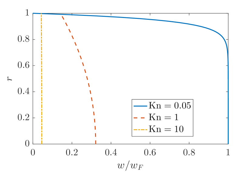
(a)

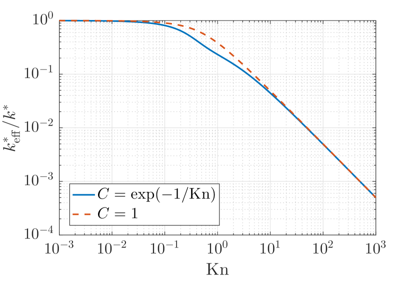
(b)

Figure 2: (a) Axial component of the heat flux according to Eqn. (14) with $C=\exp(-1/\text{Kn})$ for different values of Kn and scaled with the classical heat flux $w_{\text{F}}$. Solid, dashed and dashed-dotted lines correspond to $\text{Kn}=0.05$, $\text{Kn}=1$ and $\text{Kn}=10$ respectively. (b) The dependence of the ETC given by (16) on the Knudsen number for two choices of the function $C$.

To aid with the physical interpretation of the model solutions and their asymptotic limits, the radial dependence of the axial flux $w$ is plotted for three Knudsen numbers ($\text{Kn}=0.05$, $1$, and $10$) in Fig. 2 (a). The ETC, given by (16), is plotted as a function of the Knudsen number in Fig. 2 (b) for two choices of the function $C$. The figures make it clear that there are three distinct regimes to consider, corresponding to diffusive ($\text{Kn}\ll 1$), ballistic ($\text{Kn}\gg 1$), and mixed ($\text{Kn}=O(1)$) modes of thermal energy transport. The three values of the Knudsen number in Fig. 2 (a) are chosen to clearly illustrate how the axial flux varies across these three regimes.

For small Knudsen numbers, $\text{Kn}\ll 1$, the phonon MFP is small compared to the radius of the NW. Phonons in the bulk are therefore more likely to collide with each other before reaching the boundary of the NW and scattering. This corresponds to the boundary condition $w\to 0$ as $\text{Kn}\to 0$. Due to the relatively small influence of non-local effects, thermal energy in the bulk is transported with little resistance across the NW, with an axial flux that approximates the classical flux $w_{F}$ predicted by Fourier’s law. However, there is a thin boundary layer near the edge of the NW where the flux rapidly decreases to zero in order to satisfy the no-slip condition. The (dimensional) width of this boundary layer is $O(\ell^{*})$, reflecting the fact that boundary effects become relevant on length scales that are commensurate with the phonon MFP. As the Knudsen number tends to zero, the width of this boundary layer does so as well. The restricted transport of thermal energy in the boundary layer leads to a slight reduction in the ETC compared to its bulk value, which is captured in the small-Kn limit of $k_{\text{eff}}$ given by (19) and shown in Fig. 2 (b) by the slow reduction in $k_{\text{eff}}^{*}/k^{*}$ as Kn increases from $10^{-3}$ to $10^{-1}$.

In the limit of large Knudsen number, $\text{Kn}\gg 1$, the phonon MFP greatly exceeds the radius of the NW. Phonons therefore collide more frequently with the boundary than with each other, resulting in a substantial decrease in the flow of thermal energy. The strong influence of non-local effects and large slip length lead to an axial flux that is uniform along the radial direction and, in particular, close to its value on the boundary, $w\sim\text{Kn}^{-1}w_{F}/2$. Therefore, as $\text{Kn}\to\infty$, corresponding to an arbitrarily large MFP relative to the NW radius, the axial flux tends to zero. The restricted transport of energy in this regime results in a marked decrease in the ETC, the magnitude of which also scales linearly with $\text{Kn}^{-1}$, as demonstrated in Eqn. (18).

The proportionality between the flux $w$ and the inverse Knudsen number $\text{Kn}^{-1}$ can be understood by drawing on the analogy between nanoscale heat transfer and fluid dynamics. In the limit of large Kn (analogous to large viscosity), the net force exerted by the temperature gradient (analogous to pressure) on an arbitrary cross section of the NW must balance the net traction (i.e., shear stress) along its circumference,

$$\pi k\frac{\text{d}T}{\text{d}x}\sim 2\pi\text{Kn}^{2}\left.\frac{\partial w}{\partial r}\right|_{r=1}.$$ (20)

From Eqn. (20) it is seen that the rate of shear strain, $\partial w/\partial r$, induced by the temperature gradient is small and of size $O(\text{Kn}^{-2})$. The scaling for the flux (analogous to velocity) is determined by the slip condition (11b), yielding $w\sim\text{Kn}\,\partial w/\partial r\sim\text{Kn}^{-1}w_{F}/2$, where the rate of strain has been eliminated using (20) and $C$ has been approximated by its leading-order contribution $C\sim 1$ as $\text{Kn}\gg 1$. Thus, the scaling with $\text{Kn}^{-1}$ arises from the combination of large $O(\text{Kn})$ slip length and small $O(\text{Kn}^{-2})$ rate of strain.

The case of $\text{Kn}=O(1)$ corresponds to an intermediate regime where the length scales of the NW radius and MFP are the same order of magnitude. Boundary scattering plays an important role and the order-one slip length leads to a parabolic-like flux. Unlike the large- and small-Kn regimes, the ETC is strongly dependent on the functional form of $C$ when $\text{Kn}=O(1)$. Figure 2 (b) shows the ETC when $C=\exp(-1/\text{Kn})$ (solid line) and $C=1$ (dashed line). The former corresponds to the situation where the slip length $\ell_{s}^{*}$ is smaller than the non-local length $\ell^{*}$ (recall that $\ell_{s}^{*}=\ell^{*}C$). Taking $C=1$ implies that the slip length and MFP are equal. The exponential form of $C$ results in a slight kink near $\text{Kn}=1$. In physical terms, this kink is associated with a reduced ETC compared to the $C=1$ case and is the consequence of a smaller slip length and hence axial flux. Using $C=1$ smooths out this kink and yields higher values of the ETC due to greater slip.

4 Model validation and comparison

The prediction of the ETC is now compared against experimental data measured from Si nanowires with diameters $D^{*}=2R^{*}=37$ nm, $56$ nm, and $115$ nm at temperatures ranging from $T^{*}=50$ K up to $300$ K [14]. Evaluating the ETC prediction requires knowledge of the temperature dependence of the non-local length $\ell^{*}$ and thermal conductivity $k^{*}$. These two quantities are obtained from first principles in the KCM framework [36] using an open-source code [41] and plotted as functions of temperature in Fig. 3. The bulk MFP ranges from 55 nm to 5 $\mu$m, corresponding to Knudsen numbers between 2.98 and 262 ($D^{*}=37$ nm), 1.97 and 173 ($D^{*}=56$ nm), and 0.958 and 84.2 ($D^{*}=115$ nm). Thus, the exponential form of $C$ will be relevant when comparing the ETC prediction to the experimental data. Indeed, we find poor agreement when the the dependence of $C$ on Kn is neglected and $C$ is held at unity.

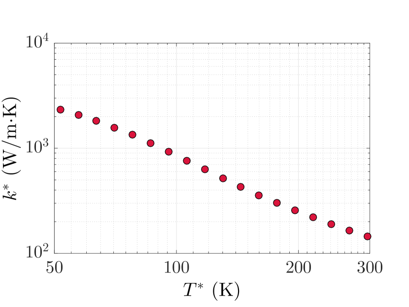
(a)

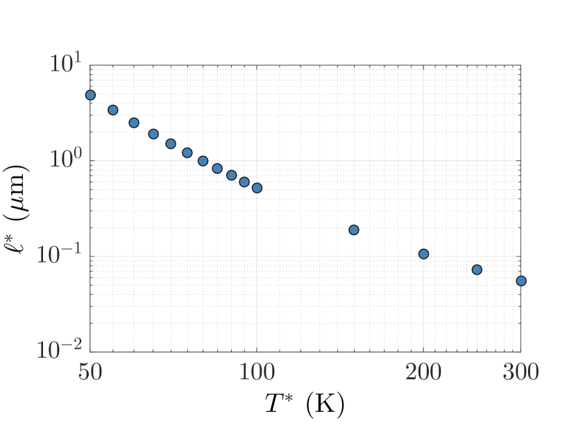
(b)

Figure 3: Temperature dependence of (a) the bulk thermal conductivity and (b) the non-local length for Si.

Figure 4 shows the ETC predicted by (16) (solid lines) and experimentally measured values of the ETC (symbols) as functions of temperature for three NW diameters (Figs. 4 (a)–(c)) and as functions of the diameter for a fixed temperature (Fig. 4 (d)). The ETC $k_{\text{eff}}^{*}$ is normalised against the bulk value $k^{*}$ to highlight the relative change that occurs as the diameter of the NW and non-local length decrease. In all cases, the theoretical predictions are in excellent agreement with the experimental data.

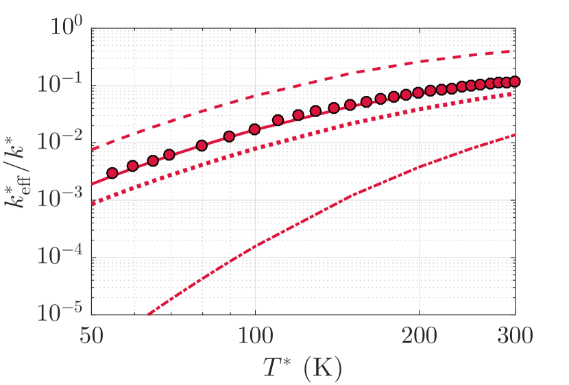
(a) $D^{*}=37$ nm.

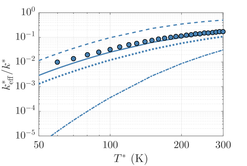
(b) $D^{*}=56$ nm.

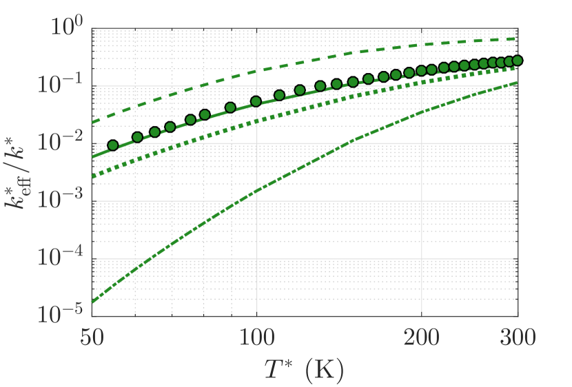
(c) $D^{*}=115$ nm.

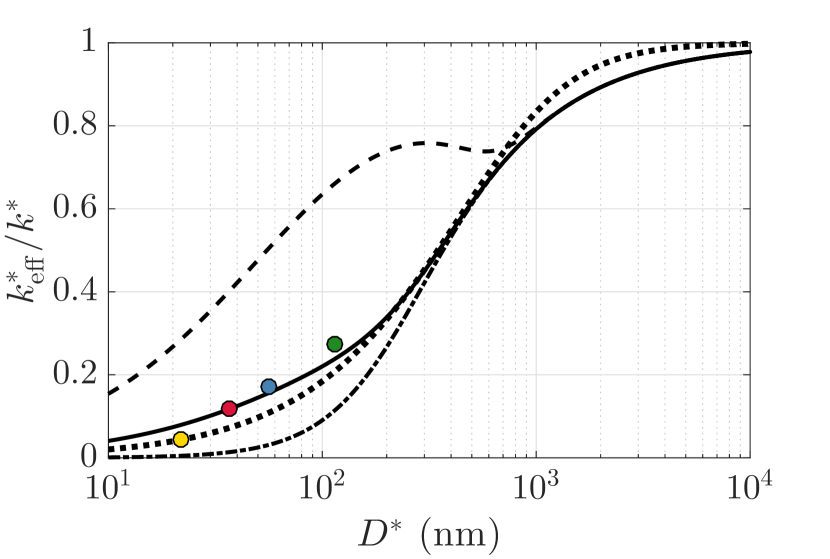
(d) $T^{*}=300$ K.

Figure 4: Comparison of theoretical predictions and experimental data for $k_{\text{eff}}^{*}$ in Si NWs of varying radii and temperature. Solid lines correspond to Eqn. (16); dashed, dotted and dashed-dotted lines represent the model predictions given by Refs. [17, 18, 35], respectively; and circles denote experimental data [14].

The dashed, dotted, and dashed-dotted lines in Fig. 4 represent theoretical predictions of the ETC computed from existing models found in Refs. [17, 18, 35], respectively. It is clear that that the model proposed here consistently yields predictions that are more representative of the experimental data. The models of Ma [17] and Dong et al. [35], both of which are based on the G-K equation, are unable to quantitatively capture the experimental data associated with all three NW diameters. These inaccuracies can be attributed to the different boundary conditions that are used in their models. Dong et al. [35] employ a no-slip boundary condition, equivalent to $C=0$ in our model. Imposing this boundary condition leads to particularly large errors at low temperatures (or large Knudsen numbers). Moreover, the calculated ETC becomes quadratically dependent on the NW radius, i.e., $k_{\text{eff}}^{*}/k^{*}\propto R^{*2}$, which contradicts the experimentally measured linear dependence between these two quantities. Ma [17] instead considers a prescribed flux on the boundary, which leads to substantial inaccuracies across the whole temperature range. The expression for the ETC presented by Alvarez and Jou [18] gives the most accurate prediction of the three existing models, although it generally underestimates the experimentally measured values. A distinguishing feature of Alvarez and Jou’s expression is that it is derived from the linearised Boltzmann equation rather than the G-K equation. This derivation does not explicitly account for the cylindrical geometry of the nanowire and thus no boundary conditions can be imposed along the outer edge, which may contribute to the errors seen in Fig. 4. In comparison to the models derived from the G-K equation, the model of Alvarez and Jou predicts that the ETC converges more rapidly to the macroscopic value with increasing NW diameter; see Fig. 4 (d). However, the lack of experimental data for microscale NW diameters prevents the models from being validated in this regime.

5 Conclusion

We have proposed a new phenomenological slip model that can be coupled with the Guyer–Krumhansl equation in order to obtain an analytical expression for the size-dependent ETC in thin nanowires. A key advantage of the proposed model is that it only requires knowledge of the bulk thermal conductivity and MFP and does not involve any fitting parameters. The prediction of the ETC of Si nanowires is found to be in excellent agreement with experimental measurements, which is particularly remarkable given the simple nature of the underlying model. When compared against existing models for the ETC, we observed that the proposed model yielded the most accurate predictions in all cases.

Crucial to the success of our model is the condition imposed on axial flux $w$ at the outer boundary of the nanowire. Similar models, but with different boundary conditions, were shown to be in poor agreement with much of the experimental data. It is surprising that the present choice, based purely on an analogy with viscous fluid flow, works so well without resorting to any parameter fitting. Consequently, in our future work, we intend to further investigate the precise form of the boundary condition and, ideally, produce an expression based on a detailed physical model.

Finally, although we focused on circular nanowires, the model could, in principle, be applied to arbitrary geometries. Analytical solutions could be sought in the case of simple geometries such as rectangular nanofilms. In the case of complex geometry, the model could be straightforwardly implemented in finite element software, enabling a broad range of scenarios to be explored.

References

- Salata [2004] OV Salata. Applications of nanoparticles in biology and medicine. Journal of nanobiotechnology, 2(1):3, 2004.
- Ahmad et al. [2012] F Ahmad, AK Pandey, AB Herzog, JB Rose, CP Gerba, and SA Hashsham. Environmental applications and potential health implications of quantum dots. Journal of Nanoparticle Research, 14(8):1038, 2012.
- Cregan and Myers [2015] V Cregan and TG Myers. Modelling the efficiency of a nanofluid direct absorption solar collector. International Journal of Heat and Mass Transfer, 90:505–514, 2015.
- Garnett et al. [2011] EC Garnett, ML Brongersma, Y Cui, and MD McGehee. Nanowire solar cells. Annual Review of Materials Research, 41:269–295, 2011.
- Liu et al. [2015] Z Liu, J Xu, D Chen, and G Shen. Flexible electronics based on inorganic nanowires. Chemical Society Reviews, 44(1):161–192, 2015.
- Ge et al. [2012] M Ge, J Rong, X Fang, and C Zhou. Porous doped silicon nanowires for lithium ion battery anode with long cycle life. Nano letters, 12(5):2318–2323, 2012.
- Chinen et al. [2015] AB Chinen, CM Guan, JR Ferrer, SN Barnaby, TJ Merkel, and CA Mirkin. Nanoparticle probes for the detection of cancer biomarkers, cells, and tissues by fluorescence. Chemical reviews, 115(19):10530–10574, 2015.
- Cahill et al. [2014] DG Cahill, PV Braun, G Chen, DR Clarke, S Fan, KE Goodson, P Keblinski, WP King, GD Mahan, A Majumdar, HJ Maris, SR Phillpot, E Pop, and L Shi. Nanoscale thermal transport. II. 2003–2012. Applied Physics Reviews, 1(1):011305, 2014.
- Buffat and Borel [1976] P Buffat and JP Borel. Size effect on the melting temperature of gold particles. Physical Review A, 13(6):2287, 1976.
- Sun and Simon [2007] J Sun and SL Simon. The melting behavior of aluminum nanoparticles. Thermochimica Acta, 463(1):32–40, 2007.
- Tolman [1949] RC Tolman. The effect of droplet size on surface tension. The Journal of Chemical Physics, 17(3):333–337, 1949.
- Xiong et al. [2011] S Xiong, W Qi, Y Cheng, B Huang, M Wang, and Y Li. Universal relation for size dependent thermodynamic properties of metallic nanoparticles. Physical Chemistry Chemical Physics, 13(22):10652–10660, 2011.
- Lai et al. [1996] SL Lai, JY Guo, V Petrova, G Ramanath, and LH Allen. Size-dependent melting properties of small tin particles: nanocalorimetric measurements. Physical Review Letters, 77(1):99, 1996.
- Li et al. [2003] D Li, Y Wu, P Kim, L Shi, P Yang, and A Majumdar. Thermal conductivity of individual silicon nanowires. Applied Physics Letters, 83(14):2934–2936, 2003.
- Wronski [1967] CRM Wronski. The size dependence of the melting point of small particles of tin. British Journal of Applied Physics, 18(12):1731, 1967.
- Shin and Deinert [2014] J-H Shin and MR Deinert. A model for the latent heat of melting in free standing metal nanoparticles. Journal of Chemical Physics, 140:164707, 2014.
- Ma [2012] Y Ma. Size-dependent thermal conductivity in nanosystems based on non-Fourier heat transfer. Applied Physics Letters, 101:211905, 2012.
- Alvarez and Jou [2008] FX Alvarez and D Jou. Size and frequency dependence of effective thermal conductivity. Journal of Applied Physics, 103(9):094321, 2008.
- Tzou [2011] DY Tzou. Nonlocal behaviour in phonon transport. International Journal of Heat and Mass Transfer, 54(1):475–481, 2011.
- Alvarez et al. [2009] FX Alvarez, D Jou, and A Sellito. Phonon hyrodynamics and phonon-boundary scattering in nanosystems. Journal of Applied Physics, 105(1):014317, 2009.
- Chang et al. [2008] C-W Chang, D Okawa, H Garcia, A Majumdar, and A Zettl. Breakdown of Fourier’s law in nanotube thermal conductors. Physical Review Letters, 101(7):075903, 2008.
- Chen et al. [2005] Y Chen, D Li, JR Lukes, and A Majumdar. Monte carlo simulation of silicon nanowire thermal conductivity. Journal of Heat Transfer, 127(10):1129–1137, 2005.
- Majumdar [1993] A Majumdar. Microscale heat conduction in dielectric films. Journal of Heat Transfer, 115(1):7–16, 1993.
- McGaughey et al. [2011] AJH McGaughey, ES Landry, DP Sellan, and CH Amon. Size-dependent model for thin film and nanowire thermal conductivity. Applied Physics Letters, 99(13):083109, 2011.
- Alvarez and Jou [2007] FX Alvarez and D Jou. Memory and nonlocal effects in heat transport: From diffusive to ballistic regimes. Applied Physics Letters, 90(8):083109, 2007.
- Callaway [1959] J Callaway. Model for lattice thermal conductivity at low temperatures. Physical Review, 113(4):1046, 1959.
- Holland [1963] MG Holland. Analysis of lattice thermal conductivity. Physical Review, 132(6):2461, 1963.
- Mingo et al. [2003] N Mingo, L Yang, D Li, and A Majumdar. Predicting the thermal conductivity of si and ge nanowires. Nanoletters, 3(12):1713–1716, 2003.
- Wang et al. [2010] M Wang, B-Y Cao, and Z-Y Guo. General heat conduction equations based on the thermomass theory. Frontiers in Heat and Mass Transfer, 1(1):1–8, 2010.
- Wang [2014] H-D Wang. Theoretical and Experimental Studies on Non-Fourier Heat Conduction Based on Thermomass Theory. Springer Theses. Springer, 2014.
- Guyer and Krumhansl [1966a] RA Guyer and JA Krumhansl. Solution of the linearized phonon boltzmann equation. Physical Review, 148(2):766, 1966a.
- Guyer and Krumhansl [1966b] RA Guyer and JA Krumhansl. Thermal conductivity, second sound, and phonon hydrodynamic phenomena in nonmetallic crystals. Physical Review, 148(2):778, 1966b.
- Jou et al. [1996] D Jou, J Casas-Vazquez, and G Lebon. Extended Irreversible Thermodynamics. Springer, 2nd edition, 1996.
- Sellito et al. [2012] A Sellito, FX Alvarez, and D Jou. Geometrical dependence of thermal conductivity in elliptical and rectangular nanowires. International Journal of Heat and Mass Transfer, 55(11):3114–3120, 2012.
- Dong et al. [2014] Y Dong, B-Y Cao, and Z-Y Guo. Size dependent thermal conductivity of si nanosystems based on phonon gas dynamics. Physica E: Low-dimensional Systems and Nanostructures, 56:256–262, 2014.
- Torres et al. [2016] P Torres, A Torello, J Bafaluy, J Camacho, X Cartoixà, and FX Alvarez. First principles kinetic-collective thermal conductivity of semiconductors. Phys. Rev. B, 95(4):165407, 2016. ISSN 2469-9950. doi: 10.1103/PhysRevB.95.165407.
- Zhu et al. [2017] C-Y Zhu, W You, and Z-Y Li. Nonlocal effects and slip heat flow in nanolayers. Scientific Reports, 7:9568, 2017.
- Sellitto et al. [2010] A Sellitto, FX Alvarez, and D Jou. Temperature dependence of boundary conditions in phonon hydrodynamics of smooth and rough nanowires. Journal of Applied Physics, 107(11):114312, 2010.
- Ockendon and Ockendon [1995] H Ockendon and JR Ockendon. Viscous flow. Cambridge University Press, 1995.
- Segura [2011] J Segura. Bounds for ratios of modified Bessel functions and associated Turán-type inequalities. Journal of Mathematical Analysis and Applications, 374(2):516–528, 2011.
- Torres [2017 (accessed August 20, 2017] P Torres. Kinetic Collective Model: BTE-based hydrodynamic model for thermal transport, 2017 (accessed August 20, 2017). URL https://physta.github.io/.