Atomic data and spectral modeling constraints from high-resolution X-ray observations of the Perseus cluster with Hitomi

Abstract

The Hitomi SXS spectrum of the Perseus cluster, with $\sim$5 eV resolution in the 2–9 keV band, offers an unprecedented benchmark of the atomic modeling and database for hot collisional plasmas. It reveals both successes and challenges of the current atomic codes. The latest versions of AtomDB/APEC (3.0.8), SPEX (3.03.00), and CHIANTI (8.0) all provide reasonable fits to the broad-band spectrum, and are in close agreement on best-fit temperature, emission measure, and abundances of a few elements such as Ni. For the Fe abundance, the APEC and SPEX measurements differ by 16%, which is 17 times higher than the statistical uncertainty. This is mostly attributed to the differences in adopted collisional excitation and dielectronic recombination rates of the strongest emission lines. We further investigate and compare the sensitivity of the derived physical parameters to the astrophysical source modeling and instrumental effects. The Hitomi results show that an accurate atomic code is as important as the astrophysical modeling and instrumental calibration aspects. Substantial updates of atomic databases and targeted laboratory measurements are needed to get the current codes ready for the data from the next Hitomi-level mission.

1 Introduction

Many major achievements in X-ray studies of clusters of galaxies were made possible by the advent of new X-ray spectroscopic instruments. The proportional counters on the Ariel V mission (spectral resolving power $R\equiv E/\Delta E\sim$ 6) revealed the highly ionized Fe line emission near 7 keV in the Perseus cluster (Mitchell et al., 1976), establishing the thermal origin of cluster X-rays. The CCDs ($R=$ 10–60) onboard the ASCA satellite further identified line emission from O, Ne, Mg, Si, S, Ar, Ca, and Ni in the hot intracluster medium (ICM: Fukazawa et al., 1994; Mushotzky et al., 1996). The Reflection Grating Spectrometer (RGS: $R=$ 50–100 for spatially extended sources) onboard XMM-Newton (Peterson et al., 2001; Tamura et al., 2001; Kaastra et al., 2001) discovered the lack of strong cooling flows in cool-core clusters. Most recently, the Soft X-ray Spectrometer (SXS: Kelley et al., 2016) onboard the Hitomi satellite (Takahashi et al., 2016) disclosed the low energy density of turbulent motions in the central region of the Perseus cluster with the resolving power of $R\sim$ 1250 (Hitomi Collaboration et al., 2016). Each iteration of higher resolution spectroscopy enhances our understanding of clusters and other cosmic objects.

As more high-resolution X-ray spectra become available, the X-ray community — including observers, theoreticians, and laboratory scientists — urgently needs accurate and complete atomic data and plasma models. As a first step in achieving this, we will compare the current data and models (collectively called “codes” hereafter). The most used plasma codes in X-ray astronomy are AtomDB/APEC (Smith et al., 2001; Foster et al., 2012), SPEX (Kaastra et al., 1996), and CHIANTI (Dere et al., 1997; Del Zanna et al., 2015). The AtomDB code descends from the original work of Raymond & Smith (1977), SPEX started with Mewe (1972), and CHIANTI started with Landini & Monsignori Fossi (1970). All these codes have evolved significantly since their initial beginnings, often stimulated by the challenges imposed by new generations of instruments. It is clear that the code comparison is strongly needed to verify the scientific output and to understand systematic uncertainties in the results originating from the codes and atomic databases. However, few code comparisons have been done (e.g., Audard et al., 2003), and in particular, so far there is no comparison based on high-resolution X-ray spectra of galaxy clusters.

The Hitomi X-ray observatory was launched on February 17, 2016. Among the main scientific instruments, the SXS has an unprecedented resolving power of $R\sim$1250 at 6 keV over a 6$\times$6 pixel array (3’$\times$3’). It has a near-Gaussian energy response with FWHM$=$4–6 eV over the 0.3–12 keV band (Leutenegger et al., in prep.). The X-ray mirror has an angular resolution with a half-power diameter of 1.2’ (Maeda et al., accepted.). A gate valve was in place for early observations to minimize the risk of contamination from out-gassing of the spacecraft (Tsujimoto et al., 2016), which includes a Be window that absorbs most X-rays below $\sim$2 keV. As the SXS is a non-dispersive instrument (unlike gratings) it can be used to observe extended objects without a loss of spectral resolution. This makes the SXS the best instrument for high-resolution spectroscopic studies of galaxy clusters. The Perseus cluster was observed as the first-light target of the SXS, and the first paper showing its spectroscopic capabilities focused on the turbulence in the Perseus cluster (Hitomi Collaboration et al., 2016).

With these data, we can also measure abundances (Hitomi Collaboration et al. 2017b: hereafter Z paper), temperature structure (Hitomi Collaboration et al. in prep.: T paper), and resonance scattering (Hitomi Collaboration et al. accepted.a: RS paper). These quantities are essential to understand the origin and evolution of galaxy clusters (see review by Böhringer & Werner 2010). Metal abundances trace products of billions of supernovae explosions integrated over cosmic time and the measurements are crucial for understanding chemical evolution of ICM as well as the evolutions and explosions of progenitor stars (Werner et al., 2008). Temperature structure or anisothermality gives an insight into thermodynamics in ICM and thus important for understanding of the heating mechanism against effective radiative cooling in a dense core region (Peterson & Fabian, 2006). Resonance scattering is another, indirect tool to assess turbulence, one of the candidate mechanisms of the ICM heating. Required precisions to these quantities depend on astrophysical objectives — for the cosmic star-formation history the Ni-to-Fe abundance ratio needs to be measured to $\approx$10% and for detection of resonance scattering with the Fe He$\alpha$ complex the forbidden-to-resonance (z-to-w) line ratio to a few percent, for instance (see individual topical papers for details).

In this paper we focus on the atomic physics and modeling aspects of the Perseus spectrum with the Hitomi SXS. We show that this high-resolution spectrum offers a sensitive probe of several important aspects of cluster physics including turbulence, elemental abundance measurements, and structures in temperature and velocity (section 3). We investigate the sensitivity of the related derived physical parameters to various aspects of the spectroscopic codes (section 4) and their underlying atomic data (section 5), spectral (section 6) and astrophysical (sections 7 and 8) modelings, as well as fitting techniques (section 9). By consolidating these systematic factors and by comparing them to statistical uncertainties as well as the systematic factors due to instrumental calibration effects (appendix C), we can evaluate with what precisions the important quantities can be determined. This allows us to be optimally prepared for future high-resolution X-ray missions. We highlight the relative changes to each parameter by using different atomic modelings and so on, rather than the changes in fitting statistics, since the former is more fundamental for understanding the systematic uncertainties in the scientific results. The astrophysical interpretation of our derived parameters is not discussed in this paper, but will be in a series of separate papers focusing in greater detail on the relevant astrophysics, e.g., abundances (Z paper), temperature structure (T paper), resonance scattering (RS paper), velocity structure (Hitomi Collaboration et al. accepted.b: V paper), and the central active galactic nucleus (AGN) of the Perseus cluster (Hitomi Collaboration et al. accepted.c: AGN paper). Also, we do not examine combined effects of different types of systematic factors (e.g., plasma-code dependence in the detailed astrophysical modeling like multi-temperature models), which will be separately discussed in the individual topical papers.

2 Data reduction

In this paper, the cleaned event data in the pipeline products version 03.01.005.005 are analyzed with the Hitomi software version 005a and the calibration database (CALDB) version 005 (Angelini et al., 2016). There are four Hitomi observations of the Perseus cluster (name: sequence number $=$ “Obs 1”: 100040010, “Obs 2”: 100040020, “Obs 3”: 100040030–100040050, and “Obs 4”: 100040060). The instrument had nearly reached thermal equilibrium by Obs 4 (Fujimoto et al., 2016), and the calibrations of Obs 2 and Obs 3 can be checked against Obs 4 because of their overlapping fields of view (FOVs), but the FOV of Obs 1 does not overlap the others and the instrument was the most out of equilibrium during that pointing. Hence only the Obs 2, 3, and 4 are used in this work.

Events registered during low-Earth elevation angles below two degrees and passages of the South Atlantic Anomaly were already excluded by the pipeline processing which created the cleaned events file. Events coincident with the particle veto had also already been rejected. Data were further screened by criteria described as “recommended screening” in the Hitomi data reduction guide to remove those with distorted pulse shapes or coincident events in any two pixels, which further reduces the background, though the difference is negligible given the surface brightness of the Perseus cluster. For all the three observations (Obs 2–4), only high-resolution primary events (an event with no pulse in the interval 69.2 ms before or after it) were extracted and used. This choice is fine because relative ratios are the same between different event types (Seta et al., 2012; Ishisaki et al., 2016).

The line broadening due to the spatial velocity gradient in the ICM is removed, since it is not relevant to the atomic study. To do this, we apply an additional energy scale correction (also used in Hitomi Collaboration et al., 2016, 2017a), forcing the strong Fe-K lines to appear at the same energy in each pixel, aligned to the same redshift as the central AGN ($z=$0.01756 or $cz=$5264 km s^-1: Ferruit et al., 1997). This also removes residual gain errors in the Fe-K band. The effect of the spatial velocity correction on the baseline-model fitting (section 3) is discussed in appendix C. A recent measurement of NGC 1275 indicates an alternative redshift of 0.017284$\pm$0.00005 (V paper). In this paper, we do not refer to the new value, since its impact on the other fitting parameters would be washed out by the non-linear energy-scale correction applied later (appendix A) or by the redshift component included in the baseline model (section 3).

The large-size redistribution matrix files (RMFs) for high-primary events created by sxsmkrmf are used to take into account the main Gaussian component, the low-energy exponential tail, and escape peaks of the line spread function (Leutenegger et al., in prep.). We have also tested two different types of RMFs; one is the small-size RMFs which includes only the Gaussian core, and the other is the extra-large–size RMFs with all components in the large-size RMFs plus electron-loss continuum. The effect of changing the RMF type is discussed in appendix C. The ancillary response files (ARFs) are generated separately for the diffuse emission and the point-source component. To enhance the precision of the diffuse ARFs, a background-subtracted Chandra image of the Perseus cluster in the 1.8–9.0 keV band whose AGN core is replaced with the average value of the surrounding regions is used to provide the spatial distribution of seed photons. Since the effective area is estimated based on the input image with a radius of 12’, which is larger than the detector FOV (3’$\times$3’), the measured spectral normalization reported in this paper is larger than the actual value. We do not correct this effect since this paper is focused on the relative uncertainties instead of the absolute values. We have further tested to use the point-source ARF for the both components, and show the effects in appendix C.

The non X-ray background (NXB) of the SXS is much lower than those of the X-ray CCDs thanks to the anti-coincidence screening, which reduces the NXB rate by a factor of $\approx$10 (Kilbourne et al., accepted.). We extract the NXB spectrum from Earth occultation data with sxsnxbgen, and screened with the standard NXB criteria and the same additional screening as the source events. The NXB spectrum is taken into account as a SPEX file model in the baseline analysis (section 3). Other background components, which include the cosmic X-ray background and Galactic foreground emission, are negligible for the Perseus data. The relative changes of the baseline parameters for a fitting in absence of the NXB is shown in appendix C.

The main remaining issue in the data analysis is that the planned calibration procedures were not fully available for these early observations. In particular, the contemporaneous calibration of the energy scale (or gain) for the detector array was not yet carried out. The previous Hitomi papers (Hitomi Collaboration et al., 2016, 2017a) focused on a relatively narrow energy range; in this work we study a wide energy band of 1.9–9.5 keV. This forces us to apply two additional corrections to the energy scale and effective area as described in appendix A.

3 Baseline model

The result of a spectral model fit is a list of parameters representing the source. These parameters depend on several factors, like the statistical quality of the data, the instrument calibration, background subtraction method, fitting techniques, spectral model components, physical processes included in the spectral model, and atomic parameters. All of these factors contribute to the final set of source parameters that is derived. Apart from the statistical uncertainties, all other factors act like a kind of systematic uncertainty, and by carefully analyzing each individual contribution we can assess its contribution to the final uncertainty.

We proceed as follows. Below we define our baseline best-fit model and explain why we incorporate each component in the model. We then list the best-fit parameters with their statistical uncertainties. The effects of the different systematic factors are in general not excessively large, and therefore we list their impact by showing by how much the best-fit parameters are increased or decreased due to these factors. Usually the statistical uncertainties on the best-fit parameters are very similar for all investigated cases, so we only list the statistical uncertainties of the baseline model.

We use the SPEX package (Kaastra et al., 1996) to define the baseline model because it allows us to test the system in a straightforward way. The version of SPEX that is being used here is 3.03.00. It calculates all relevant rates, ion concentrations, level populations, and line emissivities on the fly (see section 4.1 for more details).

We use optimally binned spectra (using the SPEX obin command structure; see appendix A.3) with C-statistics (Cash, 1979). This choice will be elaborated later (section 9).

All abundances are relative to the Lodders & Palme (2009) proto-solar abundances with free values relative to those abundances for the relevant elements.

The dominant spectral component is a collisionally ionized plasma, with a temperature of about 4 keV (Hitomi Collaboration et al., 2016), modeled with the SPEX cie model. For the ionization balance we choose the Urdampilleta et al. (2017) ionization balance (for more detail see section 5.4). The electron temperature, abundances of Si, S, Ar, Ca, Cr, Mn, Fe, and Ni are free parameters; the abundances of all other metals (usually with no or very weak lines in the bandpass of the Hitomi SXS) are tied to the Fe abundance. In addition, we leave the turbulent velocity free; the value of this turbulent velocity has been discussed in detail in Hitomi Collaboration et al. (2016). Although in SPEX the magnitude of turbulence is parameterized by a two-dimensional root-mean-square velocity $v_{\rm mic}$ assuming isotropic velocity distribution, we convert it into one-dimensional line-of-sight (LOS) velocity dispersion $\sigma_{v}$ ($=v_{\rm mic}/\sqrt{2}$) and use it throughout this paper to enable direct comparisons to the previous studies (Hitomi Collaboration et al., 2016, 2017a).

The Hitomi SXS spectrum of the Perseus cluster shows clear signatures of resonance scattering (RS paper); in addition, we may expect absorption of He-like line emission by Li-like ions (Mehdipour et al., 2015). To account for both effects, we include the absorption from a CIE plasma as modeled by the SPEX hot model to our model. The hot model calculates the continuum and line absorption from a plasma with the temperature, chemical composition, turbulent velocity and outflow velocity as free parameters. This absorption is applied to all emission components from the cluster. Because the FOV of the Hitomi SXS is relatively small compared to the size of the Perseus cluster, the effects of resonance scattering to lowest order imply the removal of photons from the line of sight towards the cluster core; we do not observe the re-emitted photons further away from the nucleus. A more sophisticated resonance scattering model is discussed by RS paper. In order not to over-constrain the model, we leave only the column density of the hot absorbing gas $N_{\rm H,hot}$ free, and tie the other parameters (electron temperature, abundances, turbulent and outflow velocities) to the values of the main 4-keV emission component (but see section 7).

Our spectrum also contains a contribution from the central AGN of NGC 1275. This is modeled by a powerlaw (SPEX component pow) plus two Gaussians (gaus) for the neutral Fe K$\alpha$ lines. We use the powerlaw model which has a 2–10-keV luminosity of 2.4$\times$10³⁶ W or a flux of 3.5$\times$10^-14 W m^-2, almost one fifth of the total 2–10-keV luminosity of the observed field, and a photon index of 1.91. The Gaussian lines have rest-frame energies of 6.391 keV and 6.404 keV, an intrinsic FWHM of 25 eV and a total luminosity of 5.6$\times$10³³ W or a total flux of 8.0$\times$10^-17 W m^-2. We have kept the parameters of the central AGN frozen in our fits to the above values. The above model and parameter values are from the initial evaluation for AGN paper, which have been updated later. Updating the AGN spectrum modeling results in slightly different best-fit values of the baseline model (section 8.3), but the changes are so small that relative differences in the ICM parameters due to other systematic factors are unchanged. Thus we use the original AGN model and parameters throughout this paper except in section 8.3.

We apply further the cosmological redshift (SPEX reds component) to the model, but leave it as a free parameter for the baseline model to account for any residual systematic energy scale corrections (either of instrumental or astrophysical origin; this is not important for the present study).

The last spectral component applied to all spectra is another hot component to account for the interstellar absorption from our Galaxy; we have frozen the temperature to 0.5 eV (essentially a neutral plasma), with a column density of 1.38$\times$10²¹ cm^-2, following the argumentation in Hitomi Collaboration et al. (2017a). The abundances are frozen to the proto-solar abundances (Lodders & Palme, 2009).

The model contains further a component of pure neutral Be and a correction factor for the effective area (see appendix A.2); these serve purely as instrumental effective area corrections and are kept frozen for our modeling.

To summarize, the baseline model starts with a thermal ICM and AGN components, self-absorbed, redshifted, absorbed again by the foreground, and corrected for instrumental effects. The free parameters of our model are then the emission measure $Y$ and temperature $kT$ of the hot gas, the turbulent velocity $\sigma_{v}$ of the hot gas, the abundances of Si, S, Ar, Ca, Cr, Mn, Fe, and Ni, the effective absorption column of the hot cluster gas $N_{\rm H,hot}$, and the overall redshift of the system $z$. This baseline model achieves a C-statistic value ($C_{\rm stat}$) of 4926 for an expected value of 4876$\pm$99.

Table 1: Parameters of the reference model and sensitivity to model assumptions. The first two lines give the best-fit values with their 1$\sigma$ statistical uncertainty. The next lines show the parameter differences of the tested models relative to the baseline model. Differences larger than 3$\sigma$ statistical uncertainty are emphasized in boldfaces.

Model	$C_{\rm stat}$	$Y$	$kT$	$\sigma_{v}$	Abundance (solar)								$N_{\rm H,hot}$	$cz$
		(1073 m-3)	(keV)	(km s-1)	Si	S	Ar	Ca	Cr	Mn	Fe	Ni	($10^{24}$ m-2)	(km s-1)
Baseline	4926.03	3.73	3.969	156	0.91	0.94	0.83	0.88	0.70	0.74	0.827	0.76	18.8	5264
Stat. error	–	0.01	0.017	3	0.05	0.03	0.04	0.04	0.10	0.15	0.008	0.05	1.3	2
Plasma codes (section 4):
Old versions of SPEX
$\ldots$ v2	1125.06	0.03	0.031	14	$-$0.13	$-$0.14	$-$0.05	$-$0.08	–	–	$-$0.026	0.11	$-$0.8	$-$6
$\ldots$ v3.00	2372.33	$-$0.08	0.263	12	0.03	0.09	0.10	0.06	$-$0.11	$-$0.12	$-$0.243	$-$0.28	$-$18.8	$-$2
APEC/AtomDB
$\ldots$ v3.0.2	670.06	0.07	$-$0.039	$-$13	$-$0.24	$-$0.21	$-$0.15	$-$0.13	$-$0.24	$-$0.39	$-$0.047	$-$0.17	$-$2.7	1
$\ldots$ v3.0.8	22.27	0.03	0.071	$-$16	$-$0.10	$-$0.07	$-$0.05	$-$0.07	0.01	$-$0.05	$-$0.134	$-$0.05	$-$7.6	$-$6
CHIANTI v8.0	327.44	0.01	0.002	4	$-$0.17	$-$0.12	0.14	$-$0.08	–	–	0.011	$-$0.04	$-$1.8	8
Cloudy v13.04	21416.07	0.74	$-$0.370	$-$7	$-$0.54	$-$0.52	$-$0.53	$-$0.46	$-$0.43	$-$0.15	$-$0.399	0.14	$-$18.8	$-$8
Atomic data (section 5):
FeXXV triplet	$-$10.68	0.00	0.003	1	0.00	0.00	0.00	0.00	0.00	0.00	$-$0.007	0.00	$-$0.4	0
ionization balance
$\ldots$ AR85	104.80	0.13	0.017	$-$3	$-$0.02	$-$0.02	$-$0.03	$-$0.02	–	–	0.017	$-$0.02	2.4	1
$\ldots$ AR92	94.65	0.09	0.021	$-$4	$-$0.02	$-$0.02	$-$0.03	$-$0.02	–	–	0.021	$-$0.03	2.0	0
$\ldots$ B09	$-$18.62	$-$0.13	0.003	$-$2	0.00	0.01	0.00	0.00	$-$0.01	$-$0.01	0.029	0.01	1.1	0
Plasma modeling (section 6):
Voigt profile	$-$8.28	0.01	$-$0.003	$-$4	$-$0.01	$-$0.01	0.00	0.00	0.01	0.00	$-$0.003	0.01	$-$1.2	1
$g_{\rm acc}$	$-$0.54	$-$0.01	$-$0.005	0	0.00	0.00	0.00	0.00	0.00	0.00	0.006	0.00	$-$0.1	0
$n_{\rm max}$	61.46	$-$0.01	0.006	$-$1	0.02	0.04	0.02	0.01	$-$0.01	$-$0.03	0.023	0.00	1.0	0
Astrophysical modeling (section 7):
$T_{\rm ion}$ free	$-$0.02	0.00	0.000	$-$1	0.00	0.00	0.00	0.00	0.00	$-$0.01	0.000	0.00	$-$0.1	0
NEI effects
$\ldots$ $RT$ free	$-$3.26	$-$0.01	0.026	$-$1	$-$0.02	$-$0.02	$-$0.01	$-$0.01	$-$0.01	$-$0.02	0.001	$-$0.01	0.7	0
$\ldots$ Ionizing	$-$5.46	$-$0.02	0.025	0	0.01	$-$0.01	$-$0.06	$-$0.06	$-$0.02	$-$0.04	0.000	$-$0.01	0.8	0
$\ldots$ Recombining	$-$9.19	0.02	$-$0.036	2	$-$0.02	$-$0.02	$-$0.01	0.00	0.03	0.02	0.000	0.01	$-$1.5	0
$\sigma_{T}$ free	$-$60.90	0.13	$-$0.139	2	$-$0.10	$-$0.10	$-$0.04	0.01	0.08	0.10	0.024	0.03	$-$2.3	0
He abund.	$-$0.07	$-$0.08	$-$0.001	0	0.02	0.03	0.02	0.02	0.02	0.01	0.025	0.02	$-$0.6	0
Spectral components (section 8):
No RS	341.02	0.05	$-$0.015	13	$-$0.05	$-$0.04	$-$0.03	$-$0.02	0.04	0.01	$-$0.094	0.01	$\equiv$0	4
Hot comp. free	$-$1.40	0.00	0.000	2	0.00	0.00	0.00	0.00	0.00	0.00	0.003	0.00	1.3	0
CX	$-$13.34	0.00	0.018	$-$3	$-$0.02	$-$0.01	0.00	$-$0.01	$-$0.01	$-$0.02	$-$0.042	0.00	$-$1.4	$-$1
AGN
$\ldots$ No AGN	624.54	0.68	0.523	4	$-$0.01	$-$0.05	$-$0.09	$-$0.14	$-$0.15	$-$0.12	$-$0.206	$-$0.16	12.8	3
$\ldots$ New AGN	8.42	0.18	0.028	0	$-$0.03	$-$0.03	$-$0.03	$-$0.04	$-$0.04	$-$0.04	$-$0.041	$-$0.03	1.3	0
Fitting techniques (section 9):
$\chi^{2}$	54.69	$-$0.01	$-$0.045	$-$1	$-$0.03	$-$0.01	0.00	$-$0.01	0.03	0.01	0.007	0.02	$-$0.6	0
$\chi^{2}$, no binning	—	$-$0.01	$-$0.206	$-$1	$-$0.12	$-$0.07	$-$0.03	$-$0.01	0.09	0.14	0.027	0.02	$-$3.1	0
Instrumental effects (appendix C):
No vel. cor.	61.70	0.00	0	13	0.00	0.00	0.00	0.00	$-$0.02	$-$0.02	0.001	0.01	1.0	$-$23
Small RMF	$-$4.42	0.01	$-$0.023	0	$-$0.01	$-$0.02	$-$0.01	$-$0.01	$-$0.01	$-$0.02	$-$0.003	0.00	$-$0.2	0
XL RMF	12.36	$-$0.02	0.035	0	0.00	0.03	0.02	0.02	0.02	0.01	0.010	0.00	0.1	0
No NXB	8.78	0.00	0.017	0	0.00	0.00	0.00	0.00	$-$0.01	$-$0.01	$-$0.003	$-$0.01	0.3	0
ARF
$\ldots$ PS	29.54	0.02	$-$0.052	0	$-$0.04	$-$0.02	0.00	0.00	0.01	0.04	0.003	0.00	$-$0.7	0
$\ldots$ No cor.	38.48	0.05	$-$0.076	1	$-$0.03	$-$0.03	$-$0.03	$-$0.03	0.02	0.05	$-$0.006	$-$0.03	$-$0.6	2
$\ldots$ Ground cor.	190.52	$-$0.16	$-$0.123	0	0.03	0.00	0.02	0.06	$-$0.04	0.02	0.017	0.04	$-$1.8	$-$1
$\ldots$ Crab cor.	13.36	$-$0.11	0.066	1	0.02	0.01	0.00	0.02	0.05	0.08	0.031	0.03	0.0	0
$\ldots$ New arfgen	$-$1.55	0.78	0.004	0	0.00	0.00	0.00	0.00	0.00	0.00	0.000	0.00	0.1	0
No gain cor.	626.73	0.01	0.003	4	$-$0.13	$-$0.06	$-$0.02	$-$0.01	$-$0.01	$-$0.01	$-$0.008	0.00	$-$0.5	14
Improved model (section 10):
	$-$146.77	–	–	–	$-$14	$-$11	$-$1	5	8	6	–	5	$-$8.3	0

Emission measure $Y$, temperature $kT$, LOS velocity dispersion $\sigma_{v}$, column density of hot-gas absorption $N_{\rm H,hot}$, and redshift $cz$.
Elemental abundance relative to the proto-solar values of Lodders & Palme (2009).
Expected value for the baseline model is 4876.

The best-fit parameters of our model are given in table 1. It is beyond the scope of this paper to discuss the astrophysical interpretation of the temperature, abundances, and resonance scattering; these are discussed in much greater detail by T, Z, and RS papers, respectively.

In the following sections, that form the core of our paper, we investigate in more detail the systematic effects that affect the best-fit parameters of this baseline model. We do so by showing in table 1 the difference in best-fit C-statistic and the best-fit model parameters, for different assumptions in our modeling. In several cases we also show the relative difference in the predicted model spectra.

We consider the following systematic effects: the plasma code that is used (section 4), the atomic database in the background (section 5), different choices for details of the plasma modeling (section 6), astrophysical modeling effects (section 7), the role of other spectral components apart from the main hot plasma (section 8), and spectral fitting techniques (section 9). Those due to instrumental calibration aspects are separately examined in appendix C.

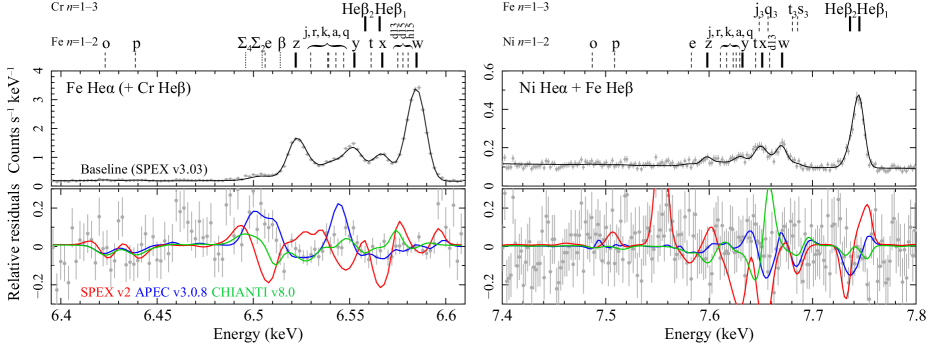
Figure 1: The Hitomi SXS spectrum in the Fe (left) and Ni (right) He$\alpha$ bands with the best-fit baseline model in the upper panels, and the residuals in the lower panels. Also shown in the lower panels are the relative difference between the baseline model and the best-fit models with various other plasma codes (SPEX v2 in red, APEC v3.0.8 in blue, and CHIANTHI v8.0 in green). Solid bars above the upper panels show energies of the main He$\alpha$ and He$\beta$ lines, while dashed and dotted ones are respectively of the Li-like and Be-like satellite lines. For the full-band results and line notations see appendices D and E, respectively.

4 Systematic factors affecting the derived source parameters: plasma code

We consider in this paper apart from SPEX version 3.03 (the baseline plasma model) also the old SPEX version 2/Mekal plasma model, the latest SPEX version before the launch of Hitomi (hereafter, the pre-launch version: SPEX version 3.00), as well as the pre-launch and the latest APEC/AtomDB versions 3.0.2 and 3.0.8 (Smith et al., 2001; Foster et al., 2012), respectively, CHIANTI version 8.0 (Dere et al., 1997; Del Zanna et al., 2015), and Cloudy version 13.04 (Ferland et al., 2013) plasma models. The best-fit models with these codes highlighting the Fe and Ni He$\alpha$ bands are compared in figure 1. The full-band results as well as the relevant atomic data are compared between these codes in appendices D and E (see also section 4.2).

4.1 SPEX versions 3.00 and 3.03

Version 3.00 of SPEX was released on January 29, 2016 as the pre-launch version for Hitomi data analysis. In SPEX version 2, line powers were calculated using the method of Mewe et al. (1985), i.e., using a temperature-dependent parameterization of the line fluxes with empirical density corrections. This version 3.00 contains fully updated atomic data for the most highly ionized ions, solving directly the balance equations for the ion energy level populations incorporating effects like density and radiation field, and uses these level populations to calculate the line power.

Triggered by the early work on the Hitomi SXS data of the Perseus cluster (Hitomi Collaboration et al., 2016), and the follow-up work as presented in this paper, several updates to version 3.00 were made leading to SPEX version 3.03, released in November 2016, that is used for the present analysis. Below we list the most important updates for the present work relative to version 3.00.

1. For Li-like ions, inner-shell transitions were extended from maximum principal quantum number $n=6$ to $n=15$ using FAC calculations.

2. A numerical issue with Be-like ions related to metastable levels was resolved allowing the full use of the new line calculations for these ions.

3. Inner-shell energy levels, Auger rates, and radiative transitions for O-like FeXIX to Be-like FeXXIII were added using Palmeri et al. (2003a).

4. A bug in the calculation of trielectronic recombination for Li-like ions was also removed; in the dielectronic capture from the He-like 1s2s level to Li-like 2s2p² levels the relative population of the 1s2s level was ignored leading to a too high population of these Li-like levels and subsequently to too strong stabilizing radiative transitions from these levels, and not in agreement with the Hitomi SXS data.

5. The proper branching ratios for excitation and inner-shell ionization to excited levels that can auto-ionize are now taken into account, leading to improvements for some satellite lines.

To demonstrate the post-launch updates, we present the results of the Hitomi SXS spectral fitting with both versions 3.00 and 3.03 in table 1. The best-fit C-statistic value increases by 2372 from version 3.03 to 3.00, and the latter gives a 7% higher temperature, 8% higher turbulent velocity, and 30% lower Fe abundance than the former one. The other abundances also have 3% to 37% deviations. The effective column density of resonance scattering $N_{\rm H,hot}$ becomes zero with version 3.00.

4.2 Using SPEX version 2 (the Mekal code)

The old Mekal code, or SPEX version 2 (Mewe et al., 1995), contained significantly fewer lines and chemical elements than the present version of SPEX. In addition, the atomic data (e.g., line energies) have been improved in the present SPEX version compared to the old Mekal model. This is evident from table 1, showing that the best-fit C-statistic value increases by 1125 if we replace the new code by the old code. A detailed comparison (figures 23–25 in appendix D) shows that there are many differences. For instance, contrary to the old model, the new model includes Cr and Mn lines (in the 5–6 keV range). Also, updates in the line energies are visible as a sharp negative residual close to a sharp positive residual.

The old code yields almost the same temperature as the new code, but there are significant changes in the derived turbulent velocity and the abundances. Small wavelength errors can be compensated for by adjusting the line broadening. Abundances are off by 2–4$\sigma$ or up to 5–15% of the values obtained from the baseline model.

This is only one example of a comparison between different models. In appendix D (figures 23–25), we show the full Hitomi SXS spectrum in 1.9–9.5 keV with our best-fit baseline model in the upper panels, and the residuals in the lower panels. In these lower panels we also show the relative difference between the baseline model and the best-fit models obtained with various other plasma codes.

The differences between these models can be divided into two classes: wavelength differences (leading to a positive residual next to a negative residual e.g., the CaXIX He$\beta$ line near 4.51 keV has a different wavelength in the Mekal code compared to the baseline model), or flux differences (leading to a strict positive or negative residual in the relative residuals e.g., the SXV forbidden line near 2.38 keV is stronger in the Mekal model compared to the baseline model).

In appendix E (tables E and 10), we list the line energies of the strongest lines in the spectrum. For comparison, the energies in SPEX are shown together with those in the APEC version 3.0.8 and CHIANTI version 8.0 codes. All the Lyman- and Helium-series transitions with model line emissivities $\geq$10^-26 photon m³ s^-1 are listed, and for satellite lines of He-like, Li-like, and Be-like ions, the threshold is set to 10^-25 photon m³ s^-1. In addition we show the Einstein coefficients and emissivities used in the three atomic codes.

4.3 APEC

APEC runs were conducted for both the pre-launch version, AtomDB version 3.0.2, and the latest version, AtomDB version 3.0.8. Since the launch of Hitomi, several updates have been made to the database to reflect the needs of the Hitomi data. These updates were not made to “fit” the Hitomi SXS data, but instead to reflect the priorities that analysis revealed. These changes were:

1. The ionization and recombination rate calculation was switched from an interpolatable grid to a fit function, which has a few percent effect on several ion populations depending on the temperatures/ion involved.

2. Wavelengths for higher $n$ transitions of the H- and He-like ions were changed to match Ritz values from the NIST Atomic Spectra Database.

3. Wavelengths for valence shell transitions of Li-like ions were changed to match Ritz values from NIST.

4. Fluorescence yields and wavelengths of inner shell lines were updated to the data of Palmeri et al. (2003a, b, 2008, 2010, 2012); Mendoza et al. (2004).

5. Collisional excitation rates for He-like Fe were changed from an unpublished data set to that of Whiteford et al. (2001).

6. Collisional excitation rates for H-like ions from Al to Ni were changed from FAC calculations to those of Li et al. (2015).

The spectral calculation is done with the BVVAPEC model in Xspec version 12.9.1 (Arnaud, 1996), while the rebinning and fitting are carried out with SPEX version 3.03.00. The abundance standard (Lodders & Palme, 2009) is applied to the APEC calculations. This allows a direct comparison between APEC and SPEX. The ionization balance calculation in APEC, on the other hand, is based on Bryans et al. (2009), while Urdampilleta et al. (2017) is used in SPEX. This difference is separately discussed in section 5.4.

The run with the pre-launch APEC version 3.0.2 gives a best-fit C-statistic which is larger than the baseline value by 670.

As shown in figure 1 and appendix D (figures 23–25), the relative difference between SPEX and APEC is usually within 10%, except for a few lines, including CrXXIII He$\alpha$, MnXXIV He$\alpha$, FeXXIV satellite lines at 6.42 keV, 6.44 keV, 8.03 keV, and 8.04 keV, NiXXVII He$\alpha$ blended with NiXXVI and FeXXIV satellite lines, and FeXXV He$\beta$ to He$\eta$ lines. Many differences might be related to the rates used in level population calculation, e.g., collisional excitation and spontaneous emission rates (see section 5 for details). The line energy data in APEC version 3.0.8 are in general good agreement with SPEX version 3.03 (see table E in appendix E for details).

As listed in table 1, the APEC code gives a similar best-fit temperature as the SPEX baseline model. The metal abundances obtained with APEC are lower by 5–10% for Si, S, Ar, Ca, and Ni than the best-fit baseline values, while the Cr abundances obtained with the two codes agree within error bars. The largest difference is with the Fe abundance, which is 16% lower in the latest APEC/AtomDB (version 3.0.8) than SPEX. The best-fit turbulent velocity in $\sigma_{v}$ (LOS dispersion) derived with the latest APEC code is 16 km s^-1 lower than the SPEX result.

4.4 CHIANTI

Another atomic code/database widely used in the UV and X-ray spectroscopy for optically thin, collisionally dominated plasma is the CHIANTI code. Compared to the APEC and SPEX codes, CHIANTI is more focused on modeling the spectra from relatively cooler plasma in the solar and stellar atmosphere, while in this work, we are testing it in the conditions of hot ICM emission. The latest version 8.0 (Dere et al., 1997; Del Zanna et al., 2015) is used. The current CHIANTI database includes all the relevant H-like and He-like ions except for Cr and Mn, which means that these abundances cannot be estimated. We calculate the collisional ionization equilibrium spectrum using an IDL-version isothermal model, setting the ionization balance to Bryans et al. (2009), and change the solar abundance table to Lodders & Palme (2009) proto-solar values. To perform the fit to the data, the IDL calculation is implemented as an input to the user model in SPEX, and the fitting engine of SPEX repeatedly triggers the IDL run until a best-fit is reached. Since the CHIANTI code does not provide line broadening information, we apply a multiplicative SPEX Gaussian broadening model vgau to the CHIANTI model. This is only a first-order approximation, since the thermal broadening should vary with the atomic number. A detailed comparison on the best-fit spectra shown in appendix D (figures 23–25) reveals several differences in emission features from the baseline model, at levels ranging from a few % up to about 20%. Most of these differences are traced back to the different input atomic data, which can be found in appendix E (tables E–10).

The C-statistic value increases by 327 when fitting with the CHIANTI code. The best-fit temperature, emission measure, turbulent velocity, and the Fe abundance are roughly consistent with the baseline results, while the remaining abundances differ by 3–19%. The required column density for resonance scattering is reduced by 10% with the CHIANTI model.

4.5 Cloudy

The Cloudy code has been developed as a tool to calculate photoionized plasmas and it is principally used for this application. It does, however, have a module for calculating CIE plasma spectra, so we have therefore fitted the Perseus spectrum with the coronal equilibrium model of Cloudy version 13.04. The abundance standard is set to Lodders & Palme (2009). Since the Cloudy code does not provide the thermal and turbulent broadening, we again apply a multiplicative SPEX Gaussian broadening model vgau to the Cloudy calculations. As shown in table 1, the fit with Cloudy yields a large C-statistic. The most significant residuals appear at the FeXXV He-series and FeXXVI Ly$\alpha$ lines. The best-fit temperature agrees with the results of the other codes, but the abundance values differ strongly from those derived from the other codes. We again note that modeling of collisional plasmas is not Cloudy’s main purpose.

5 Systematic factors affecting the derived source parameters: atomic data

As shown in table 1, the atomic code uncertainty contributes the main uncertainty of many parameters, such as the Si, S, Ar, Ca, Mn, Fe, and Ni abundances, the hot absorption, and the turbulent velocity. The code uncertainty mainly comes from the input atomic data, for instance, the ionization balance, collision excitation/de-excitation rates, recombination rates, and transition probabilities. In this section, we explore and describe the discrepancies between the current atomic data used in each code, and estimate the propagated errors on the fitted parameters.

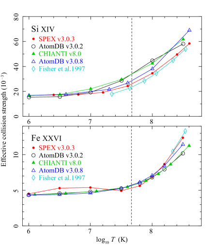
Figure 2: Comparisons of effective collision strength as a function of balance temperature. The Ly$\alpha$1 and Ly$\alpha$2 transitions are combined. The vertical dashed lines mark a temperature of 4 keV.

Table 2: Electron effective collision strengths ($10^{-3}$) of the Ly$\alpha$ transitions for a CIE plasma at 4-keV temperature.

Ion Ly$\alpha_{1}$ transition: 1s (²S_1/2) – 2p (²P_3/2) Diff. SPEX v3.03 AtomDB v3.0.8 AtomDB v3.0.2 CHIANTI v8.0 FAC SiXIV 17.11 18.97 22.12 22.14 18.80 23% SXVI 12.31 13.30 15.32 15.39 13.10 20% ArXVIII 9.29 9.74 11.07 8.08 9.59 27% CaXX 7.25 7.40 8.25 8.08 7.27 14% CrXXIV 4.61 4.68 5.00 — 4.56 11% MnXXV 4.17 4.24 4.47 — 4.12 10% FeXXVI 3.51 3.85 3.76 3.71 3.74 9% NiXXVIII 3.18 3.21 3.27 3.28 3.12 7% Ion Ly$\alpha_{2}$ transition: 1s (²S_1/2) – 2p (²P_1/2) Diff. SPEX v3.03 AtomDB v3.0.8 AtomDB v3.0.2 CHIANTI v8.0 FAC SiXIV 8.55 9.54 11.15 11.05 9.48 23% SXVI 6.15 6.68 7.75 7.68 6.63 21% ArXVIII 4.64 4.92 5.62 4.57 4.86 19% CaXX 3.62 3.74 4.20 4.03 3.71 16% CrXXIV 2.30 2.38 2.57 — 2.34 13% MnXXV 2.09 2.16 2.31 — 2.13 13% FeXXVI 1.66 1.97 1.90 1.89 1.93 16% NiXXVIII 1.59 1.65 1.70 1.64 1.62 10%

Relative differences between the codes defined as (maximum$-$minimum)$/$maximum.

5.1 Collisional excitation

5.1.1 H-like ions

In this section, we address the systematic uncertainties on the collisional excitation rates for H-like ions from the ground to the 2p levels. The radiative relaxation from the 2p levels back to the ground produces the Ly$\alpha$ lines. As shown in table 2, the effective collision strengths of SiXIV and FeXXVI for a 4-keV plasma often differ by 10–30% among atomic codes, which contributes an important uncertainty in the abundance measurement (table 1). The collision rates used in AtomDB version 3.0.2 and CHIANTI version 8.0 are systematically larger than those in SPEX version 3.03 and AtomDB version 3.0.8, while the latter two are roughly consistent with the calculations by the Flexible Atomic Code (FAC, Gu, 2008), version 1.1.1. FAC can calculate both atomic structure and scattering data, and the relativistic effects are fully taken into account by the Dirac-Coulomb Hamiltonian. By solving the configuration-interaction wave functions in the Dirac-Fock-Slater central-field potential, it evaluates the radiative transitions and auto-ionization rates for the input atomic levels, and computes the effective collisional strengths using a distorted-wave approximation. The FAC values shown are based on calculations with a default grid that contains 6 grid points. As check a calculation with a grid of 11 points has also been carried out. The values of the 11 point grid are about 5% lower than the values of the default grid calculation. The consistency between FAC and AtomDB version 3.0.8 is expected, since the AtomDB values are essentially taken from a FAC calculation by Li et al. (2015).

The differences in the effective collision strengths depend on the electron temperature. In figure 2, we compare five sets of calculations for SiXIV and FeXXVI Ly$\alpha$ transitions. For SiXIV, SPEX uses a R-matrix calculation by Aggarwal & Kingston (1992), which is roughly consistent with the AtomDB and CHIANTI values within 8% at 10⁶ K, but becomes lower by 30% at 10^7.7 K than the CHIANTI data. This means that even for the simplest H-like ions, the atomic data for the collision process are not sufficiently converged to match the accuracy of the current observations. Since the Si abundance is mostly determined by the SiXIV Ly$\alpha$ for the Hitomi SXS data, the 30% uncertainty in the collision strength calculation indicates a roughly similar error in the abundance measurement.

For FeXXVI, we compare two representative calculations using a R-matrix method, Ballance et al. (2002) (implemented in CHIANTI version 8.0 and AtomDB version 3.0.2) and Kisielius et al. (1996) (used in SPEX version 3.03), and the FAC calculation in AtomDB version 3.0.8. The three results roughly agree with each other at 10⁶ K, while the calculations of Kisielius et al. (1996) is higher than the other two up to 10⁷ K, and decreases rapidly beyond this temperature, relative to the others. At the high temperature end (3$\times$10⁸ K), the difference between the Ballance et al. (2002) and Kisielius et al. (1996) values is about 30% for the 1s (²S_1/2) – 2p (²P_3/2) Ly$\alpha_{1}$ transition. According to Ballance et al. (2002), the differences at low and high energies are mainly caused by the treatment of radiation damping and the high-energy approximation, respectively. This would contribute a minor part of the uncertainty on the Fe abundance measured with the Hitomi SXS data; the main uncertainty comes from the He$\alpha$ transitions (section 5.1.2).

5.1.2 He-like ions

We now turn to the He-like Fe-K multiplet as a test case to assess the flux errors on model lines by the input atomic data. First we define the range of related atomic levels and data in figure 3 and table 3. The most dominant populating process for the upper levels of the resonance and intercombination transitions is electron-impact excitation from the ground state, and the main loss process is radiative transition back to the ground state. The upper level of the x line (2p ³P₂) has a 18% chance to form a two-step decay via an intermediate level.

Meanwhile, for a 4-keV plasma, the upper level of the FeXXV forbidden transition (z) is populated almost equally by: excitation from the ground state; cascades from the 2p (³P₀), 2p (³P₂), and 3p (³P₂) levels; and radiative recombination from the continuum state. In addition, inner-shell ionization of FeXXIV drives 8%, and radiative transitions from the 3p (³P₁) and 4p (³P₂) levels both provide 4% of the population. The metastable level can decay to the ground only via radiative transitions.

Table 3: FeXXV He$\alpha$ multiplet formation for a CIE plasma at 4-keV temperature.

Transition	Rel. contrib.	Electron effective collision strength (10-3)					Diff.
		SPEX v3.03	AtomDB v3.0.8	AtomDB v3.0.2	CHIANTI v8.0	Open-ADAS
1 $\rightarrow$ 2	19%	0.268	0.295	0.410	0.425	0.246	42%
1 $\rightarrow$ 3	69%	0.138	0.143	0.144	0.146	0.135	8%
1 $\rightarrow$ 4	77%	0.715	0.721	0.728	0.721	0.868	18%
1 $\rightarrow$ 5	67%	0.692	0.703	0.714	0.740	0.695	6%
1 $\rightarrow$ 6	91%	4.047	4.026	4.051	4.004	4.316	7%
1 $\rightarrow$ 7	71%	0.161	0.163	0.162	0.162	0.166	3%
1 $\rightarrow$ 8	63%	0.173	0.178	0.180	0.182	0.165	9%
1 $\rightarrow$ 9	62%	0.071	0.069	0.071	0.072	0.073	5%
Transition	Rel. contrib.	Transition probability (s-1)					Diff.
		SPEX v3.03	AtomDB v3.0.8	AtomDB v3.0.2	CHIANTI v8.0	FAC
2 $\rightarrow$ 1 (z)	100%	2.080$\times 10^{8}$	1.930$\times 10^{8}$	left	2.080$\times 10^{8}$	1.997$\times 10^{8}$	7%
4 $\rightarrow$ 1 (y)	100%	4.260$\times 10^{13}$	3.720$\times 10^{13}$	left	4.350$\times 10^{13}$	4.196$\times 10^{13}$	14%
5 $\rightarrow$ 1 (x)	82%	6.550$\times 10^{9}$	6.578$\times 10^{9}$	6.519$\times 10^{9}$	6.480$\times 10^{9}$	6.568$\times 10^{9}$	1%
6 $\rightarrow$ 1 (w)	100%	4.565$\times 10^{14}$	4.670$\times 10^{14}$	left	4.610$\times 10^{14}$	4.679$\times 10^{14}$	2%
7 $\rightarrow$ 1	63%	1.524$\times 10^{13}$	1.060$\times 10^{13}$	left	1.126$\times 10^{13}$	1.248$\times 10^{13}$	30%
3 $\rightarrow$ 2	100%	3.820$\times 10^{8}$	2.770$\times 10^{8}$	left	3.740$\times 10^{8}$	3.743$\times 10^{8}$	27%
5 $\rightarrow$ 2	18%	1.470$\times 10^{9}$	1.420$\times 10^{9}$	left	1.420$\times 10^{9}$	1.466$\times 10^{9}$	3%
7 $\rightarrow$ 2	34%	8.078$\times 10^{12}$	7.990$\times 10^{12}$	left	7.861$\times 10^{12}$	8.057$\times 10^{12}$	3%
8 $\rightarrow$ 2	100%	8.932$\times 10^{12}$	8.550$\times 10^{12}$	left	8.682$\times 10^{12}$	8.660$\times 10^{12}$	4%
9 $\rightarrow$ 2	74%	3.957$\times 10^{12}$	3.550$\times 10^{12}$	left	3.642$\times 10^{12}$	3.769$\times 10^{12}$	10%

Energy-level IDs correspond to the energy levels as denoted in figure 3.
Relative contributions to the total gain or loss term of the level derived with SPEX v3.03.
Relative differences between the codes defined as (maximum$-$minimum)$/$maximum.

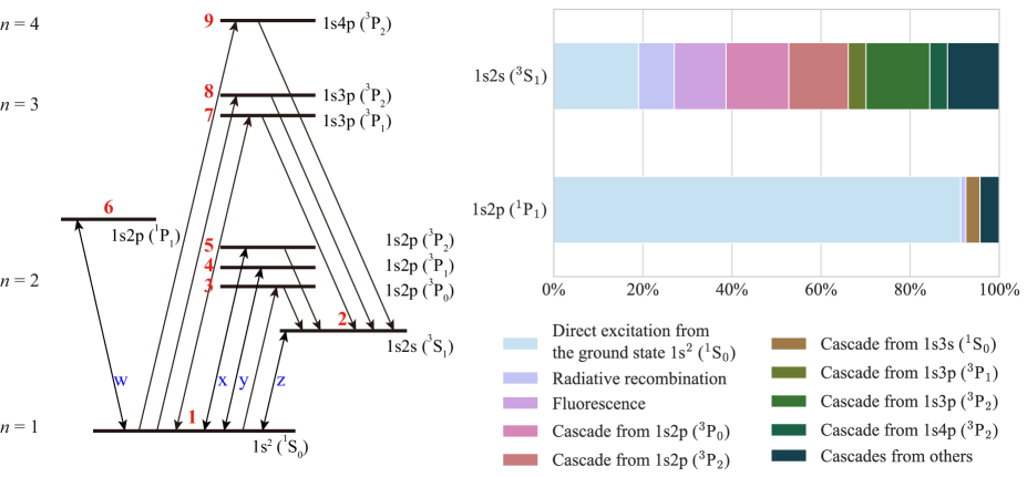
Figure 3: (left) Grotrian diagram of the dominant FeXXV levels to the triplet formation. Red numbers are used in table 3. Blue labels show transitions corresponding to the individual lines of the triplet. The 1s2s (¹S₀) level is not shown here, as it does not contribute to line production but to continuum emission via the two-photon decay (e.g., Nussbaumer & Schmutz, 1984). (right) Relative contributions to the formations of 1s2s (³S₁) and 1s2p (¹P₁) levels (upper levels of z and w, respectively).

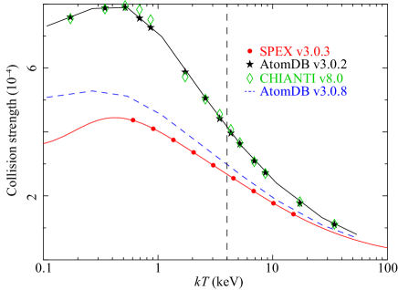
Figure 4: Comparison of the effective collision strength from the ground to 1s.2s (³S₁) state. The vertical line shows a temperature of 4 keV.

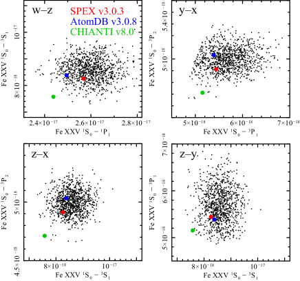
Figure 5: Monte-Carlo simulations on the four FeXXV He$\alpha$ lines. The SPEX, AtomDB, and CHIANTI values are shown in red, blue, and green, respectively. The line intensities are given in the unit of photon cm³ s^-1.

We compare the atomic data extracted from the SPEX, AtomDB, and CHIANTI databases, as well as the collision data from the Open-ADAS database, and the radiative transition data from the FAC calculation. The effective collision strengths used in SPEX, AtomDB version 3.0.2 and CHIANTI version 8.0, and AtomDB version 3.0.8 are taken from the published data in Zhang & Sampson (1987, distorted wave), Whiteford (2005, R-matrix), and Whiteford et al. (2001, R-matrix), respectively. The data from Open-ADAS is calculated with the distorted-wave approximation. We do not show the FAC results on the collisional excitation, since it does not provide explicitly the contributions from resonance excitation channels, which are incorporated in the other calculations.

As shown in table 3, the collision data converge relatively well ($<$18%) on the ground to ¹P and ³P level transitions, but differ by up to 42% on the ground to ³S transition. As shown in figure 4, the effective collision strengths used in CHIANTI version 8.0 / AtomdB version 3.0.2 are systematically larger than that in the SPEX version 3.03, by a factor of two at 1 keV, and about 40% at 10 keV. The values in AtomDB version 3.0.8 lie in the middle, about 10% higher than the SPEX values at 4 keV. It appears that the R-matrix calculations (AtomDB and CHIANTI) are systematically higher, by 10–40%, than the distorted-wave calculations (SPEX and Open-ADAS). Since the forbidden transition from ³S to the ground gives a line intensity only second to the resonance line for a 4-keV plasma, while the latter is subject to resonance scattering (section 8.1), the uncertainty of the ³S excitation should contribute a significant portion of the total error of the Fe abundance. The radiative transition data used in different codes agree within a 15% level for the He-like triplet lines. The transition rates from higher levels (e.g., $n=$3 and 4) to the ground can have a larger uncertainties up to 30%, which will be discussed in more detail in section 5.2.

Assuming that the deviations between different data gives a rough measure of the atomic process uncertainties, we carry out a Monte-Carlo simulation to quantify the atomic uncertainties on the He-like triplet line ratios. We generate 1000 sets of collisional excitation rates by randomizing based on the five sets of collision data in table 3. The same is done for the transition probability. Then we run the SPEX calculation repeatedly, each time with one set of randomized collision and radiative data, to determine the flux error on each individual line. There are two potential caveats: first, the Monte-Carlo method assumes that all the rate errors are independent, which is not always true for the atomic calculations; second, the differences between SPEX and other codes on the atomic data of the recombination processes and the fluorescent yields, as well as on the atomic structure such as the maximum principal quantum number, are not taken into account in the simulation. Therefore the error obtained in the simulation should be regarded as a lower limit.

The results of the 1000 simulations are shown in figure 5. The simulation predicts that the resonance (w), intercombination (x and y), and the forbidden (z) lines have uncertainties of $\sim$4%, 2% and 8%, and 6%, respectively. The y and z lines have the larger atomic uncertainties than the other two, probably caused by the relatively large errors of the collision strengths and the complex formation of the ³P and ³S levels. The actual AtomDB version 3.0.8 and SPEX version 3.03 line intensities indicate similar uncertainties. The CHIANTI version 8.0 triplet line fluxes are systematically lower than the simulation results and the other two codes. This could be caused by the fact that CHIANTI has the lowest maximum principal quantum number, and hence possibly a lowest radiative decay contribution to the $n=$2 levels, among the three atomic codes. When multiplying the CHIANTI fluxes by a factor of 1.05, they become well in line with the simulation results.

5.1.3 Best fit with adjusted line ratios for the x and y lines

We have tested the sensitivity of our results on the He-like Fe lines further as follows. We made the intensity of the x and y lines relative to the forbidden line a free parameter. Technically, this was achieved by applying two line components to the x and y line. This model produces the transmission $T(E)$ for in our case an absorption or emission line as $T(E)=\exp{[-\tau_{0}\phi(E)]}$ with $\phi(E)$ the Gaussian optical depth profile. We have frozen the line energy of this absorption line to the energies of the x and y lines, respectively, and the width to the width of the emission line (using the best-fit thermal and turbulent broadening from the baseline model). Thus, the only two additional free parameters are the nominal optical depths $\tau_{0}$ of both lines, positive values indicating lower flux, negative values higher flux. The best-fit parameters are $\tau_{0}=$0.035$\pm$0.028 for x and $\tau_{0}=-$0.068$\pm$0.025 for y. From this we derive that for the best-fit model the flux of the x-line should be lower by 3$\pm$3% and that of y should be higher by 8$\pm$3% compared to our SPEX plasma model in order to give the best agreement with the observed spectrum (table 1).

The atomic uncertainties on the x, y, and z lines are calculated using a Monte-Carlo simulation in section 5.1.2. Based on the simulated data, we further estimate that the errors on the x and y relative to the forbidden line ratios are 6.2% and 9.2%, respectively. Hence the best-fit modifications to the x and y lines are well in line with the expected atomic errors.

5.2 Transition probability

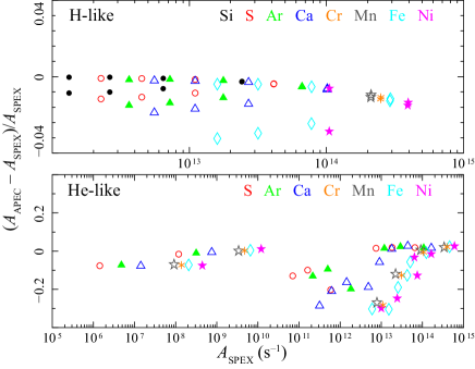
Figure 6: The differences of Einstein $A$ values of the strongest transitions (table E) in SPEX v3.03 and AtomDB v3.0.8 for the H-like (upper) and He-like (lower) ions. The upper states are in the range of $n=$2–5 for H-like and 2–4 for He-like ions.

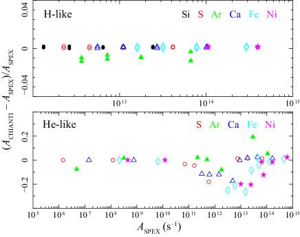
Figure 7: Same as figure 6, but for comparison between SPEX v3.03 and CHIANTI v8.0.

Besides the radiative transition data for the He-like triplet shown above, here we make a more systematic comparison of the transition probabilities among the atomic codes. The radiative data for selected strong lines are shown in appendix E (table E). In figures 6 and 7, we demonstrate that the Einstein $A$ values for H-like ions are consistent within a few percent among the codes, while for He-like ions, especially for transitions from $n=$3 or more to the ground, the $A$ values have larger uncertainties up to 30%. The SPEX $A$ values are systematically higher than those in AtomDB and CHIANTI. Partly owing to the difference in the transition data, the He$\beta$, He$\gamma$, and He$\delta$ line intensities calculated by SPEX are higher than the AtomDB and CHIANTI lines (see details in table E). These lines contribute a minor role in the abundance measurements.

5.3 Satellite line emission

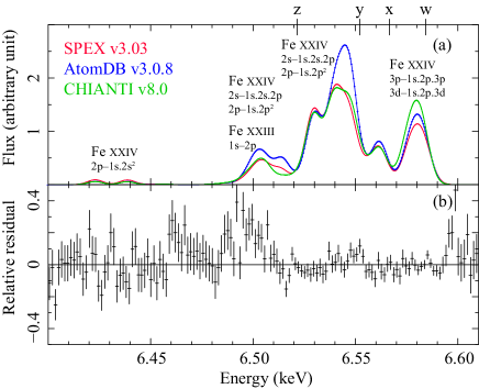
Figure 8: (a) Li-like FeXXIV and Be-like FeXXIII lines of a 4-keV CIE plasma in the 6.4–6.61 keV band. The observed line broadening is taken into account. (b) Residual of the Hitomi SXS spectrum to the baseline fit in the same band.

Table 4: Energies, Auger transition rates, and branching ratios of FeXXIV.

Level Energy Auger transition rate (s^-1) Branching ratio for radiative transition (keV) SPEX v3.03 AtomDB v3.0.8 SPEX v3.03 AtomDB v3.0.8 1s.2s^{2 2}S_1/2 6.60040 1.46$\times$10¹⁴ 1.43$\times$10¹⁴ 0.12 0.12 1s.2s.(³S).2p ⁴P_1/2 6.61369 7.79$\times$10¹⁰ 1.33$\times$10¹⁰ 0.98 1.00 1s.2s.(³S).2p ⁴P_3/2 6.61666 7.23$\times$10¹¹ 3.91$\times$10¹¹ 0.96 0.98 1s.2s.(³S).2p ⁴P_5/2 6.62781 3.53$\times$10⁴ 1.97$\times$10⁹ 1.00 0.76 1s.2s.(¹S).2p ²P_1/2 6.65348 3.89$\times$10¹³ 4.24$\times$10¹³ 0.89 0.88 1s.2s.(³S).2p ²P_3/2 6.66194 5.70$\times$10⁸ 1.41$\times$10¹¹ 1.00 1.00 1s.2p^{2 4}P_1/2 6.67097 2.41$\times$10¹¹ 3.37$\times$10¹¹ 0.99 0.99 1s.2s.(³S).2p ²P_1/2 6.67644 8.18$\times$10¹³ 6.77$\times$10¹³ 0.69 0.73 1s.2s.(¹S).2p ²P_3/2 6.67915 1.10$\times$10¹⁴ 1.07$\times$10¹⁴ 0.01 0.04 1s.2p^{2 4}P_3/2 6.67928 8.46$\times$10¹¹ 9.66$\times$10¹¹ 0.92 0.92 1s.2p^{2 4}P_5/2 6.68498 2.27$\times$10¹³ 2.61$\times$10¹³ 0.60 0.58 1s.2p^{2 2}D_3/2 6.70268 1.29$\times$10¹⁴ 1.25$\times$10¹⁴ 0.74 0.74 1s.2p^{2 2}P_1/2 6.70458 9.93$\times$10¹¹ 9.39$\times$10¹¹ 1.00 1.00 1s.2p^{2 2}D_5/2 6.70902 1.39$\times$10¹⁴ 1.37$\times$10¹⁴ 0.60 0.6 1s.2p^{2 2}D_3/2 6.72236 3.48$\times$10¹³ 3.28$\times$10¹³ 0.95 0.95 1s.2p^{2 2}S_1/2 6.74147 2.53$\times$10¹³ 2.92$\times$10¹³ 0.91 0.9

Energy levels above the ground state in SPEX v3.03.

The line energies, radiative transitions, and emissions of the satellite lines for a 4-keV CIE plasma are compared in table 10 in appendix E. The atomic level-dependent Auger transition rates and radiative-to-total branching ratios are shown in table 4, and the resulting line spectra for Fe are plotted in figure 8. The most noticeable issue is that APEC version 3.0.8 gives higher FeXXIV fluxes at $\sim$6.5 keV and 6.545 keV than the other two codes, which is driven by a recent update of APEC by incorporating the dielectronic recombination (DR) rates and branching ratios calculated in Palmeri et al. (2003a). This could partially explain the different Fe abundances with SPEX and APEC as shown in table 1.

5.4 Ionization equilibrium concentrations

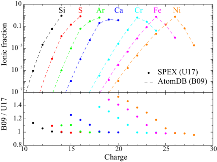
Figure 9: (upper) Ionic fraction of a 4-keV CIE plasma in SPEX v3.03 (U17: dots) and APEC v3.0.8 (B09: curves). (lower) Ratios between the two.

Figure 9 shows relative ionic fractions of a 4-keV CIE plasma based on the SPEX and APEC calculations. In SPEX the ionization balance mode was set to Urdampilleta et al. (2017) which allows to include inner-shell ionization contributions to the spectrum, while in APEC the balance from Bryans et al. (2009) was assumed. For He-like, H-like, and bare ions of Si–Cu, these two calculations agree with each other within 5%. For Li-like ions, they agree within 10%. For higher sequences, however, larger differences are seen as the APEC values are systematically larger, by up to 57%, than the SPEX values.

Here we assess the uncertainties on ionization concentration by replacing the baseline Urdampilleta et al. (2017, hereafter U17) balance with historical ones, namely Arnaud & Rothenflug (1985, AR85), Arnaud & Raymond (1992, AR92), and Bryans et al. (2009, B09). It should be noted that the AR85 and AR92 balances do not include trace elements, such as Cr and Mn. As shown in table 1, the baseline model with the AR85 and AR92 ionization balances becomes much worse by $\delta C_{\rm stat}$ of about 100, and the best-fit temperature and abundances changes by 1–3%. The B09 balance provides an equally good fit as the U17 one, yielding almost the same parameters except for the Fe abundance, which increases by 4%. The $N_{\rm H}$ of the self-absorption component changes by 6–13% for different balances. By comparing the values from the mostly used B09 and U17 balances, the systematic uncertainty on abundances from ionization concentration is 1–4%.

Figure 10: (upper) He-like to H-like ion ratio as a function of nuclear charge $Z$ for a 4-keV plasma. The solid line shows a polynomial fit in logarithm space. (lower) Relative residuals of a polynomial fit.

A related issue is the uncertainty on the He-like to H-like ion ratios. As shown in appendix D (figures 23–25), the He- and Ly-series are the dominant line feature of the Perseus spectrum, and their ratios largely determine the temperature measurement. Here we examine the He-like to H-like ion ratios as a function of nuclear charge $Z$, which is expected in theory to be a perfectly smooth function. The calculation is based on SPEX version 3.03. As shown in figure 10, the He-like to H-like ion ratio indeed appears as a nearly linear function in logarithmic space, and the scatter is within 0.5%.

6 Systematic factors affecting the derived source parameters: plasma modeling

Although it is in principle straightforward to calculate a spectrum from the atomic data, practically these calculations are based on a range of approximations, and usually include only limited physical processes — treatment of specific physical processes is limited or missing entirely. This section explores these technical issues in the plasma modeling and discusses their impacts on the fitted parameters.

6.1 Voigt profiles

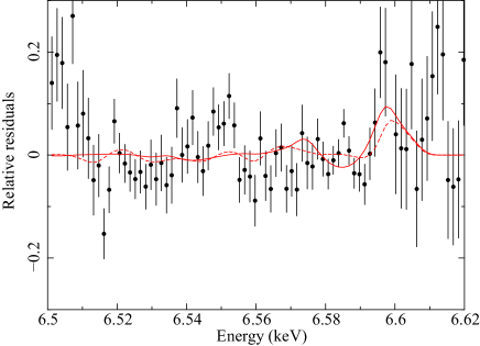
Figure 11: Residuals of the baseline model near the He-like 1s-2p transitions. The dotted curve shows the predicted model change when instead of Doppler profiles Voigt profiles are chosen, but without altering the parameters of the baseline model. The solid curve shows the same but after refitting the spectrum.

In our baseline model we have approximated the line profiles using Doppler profiles (Gaussians). This gives a significant increase in speed in obtaining our spectral fits. However, the true profiles are Voigt profiles. We have tested the sensitivity of our results to these intrinsic line profile assumptions. The Lorentzian widths of the Voigt profiles are fixed to the natural widths in SPEX version 3.03. Figure 11 shows our results. The changes are substantial (5–10%) near the FeXXV resonance line observed at 6.60 keV. In all other parts of the spectrum the changes are smaller, due to the fact that the lines are weaker.

6.2 Continuum contributions from heavy elements

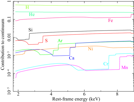
Figure 12: Relative contribution of the different elements to the continuum emission of the main thermal component in the Perseus cluster.

Not only abundant elements like H, He, O, and Fe contribute significantly to the continuum emission, but also the contributions of less abundant elements like Cr or Mn are detectable. We discovered this by accident when we tested our baseline model with the old version of SPEX (version 2). In that old version only the 15 most abundant elements with nuclear charge less than 30 were taken into account in the line emission, yet the model could produce some very crude constraints on the Cr and Mn abundance, while the line emission of both elements was not accounted for by the model.

What is the explanation for this? In figure 12 we show the relative contribution of each element to the continuum emission (including here also the AGN continuum). About 90% of the emission is due to H and He, about 10% is due to Fe, and all other elements contribute less than a few percent at most. In particular for the elements between Si and Mn clearly the smooth two-photon emission bumps and the free-bound edges are visible.

The present spectrum has 487621 counts with a nominal uncertainty of 698 counts. Cr and Mn contribute 78 and 104 counts to the continuum, respectively. Therefore their contribution is small but if the abundances would have been off by a factor of 10, their continuum contribution with their specific structure as shown in figure 12 would have allowed to constrain their abundances.

In SPEX all contributions to the radiative recombination (free-bound) continuum smaller than a threshold are omitted for computational efficiency (the free-bound continuum calculation takes most of the computing time for high-resolution spectra because of the large number of energy bins and atomic shells that need to be calculated). The threshold is controlled by the parameter ”gacc” that can be set by the user. Its default value is 10^-3, but for figure 12 we have put it to 10^-7.

This same value is used in the entry $g_{\rm{acc}}$ listed in table 1. It can be seen that changing this parameter has only a very minor effect on the fit (improvement of C-statistic only 0.41), but the additional computational burden is heavy.

6.3 Maximum principal quantum number $n$ in the calculations

Collisional excitation by thermal electrons mostly populates the inner shells of the atomic structure. Although the emission lines from outer shells are usually rather weak, some of them become visible in the Hitomi SXS spectrum (appendix E; table E). Here we test the impact on the obtained spectral parameters by limiting the maximum principal quantum number $n$ in the calculation. As shown in table 1, when excluding the outer shells with $n>5$, the fitting with the baseline model gets poorer by $\delta C_{\rm stat}\approx$61, and the best-fit metal abundances become slightly larger by a few percent. This is because the outer shell population will also contribute to the inner shell (e.g., Ly$\alpha$, Ly$\beta$) transitions by radiative cascading. As shown in table E, the Hitomi SXS data require the plasma code to calculate to at least $n=10$ for the FeXXV lines.

6.4 Hyperfine mediated transitions

The isotopic composition of Fe contains approximately 2% of ⁵⁷Fe, which has non-zero nuclear spin and thus might be expected to exhibit a hyperfine-mediated transition from 1s2p ³P₀ to ground, resulting in a weak third intercombination line. The transition rate has been calculated by Johnson et al. (1997), who find that it is about 6% of the transition rate to the 1s2s ³S₁ state, so that the strength of the 1s2p ³P₀ transition to ground is negligible for Fe. The low branching ratio to ground can be attributed to the relatively weak magnetic moment of ⁵⁷Fe. We caution that all odd $Z$ elements have non-zero nuclear magnetic moments, and for most of those ions in the Fe group, the hyperfine mediated decay channel to ground is actually dominant.

7 Systematic factors affecting the derived source parameters: astrophysical model

The atomic data and plasma code are eventually integrated into the spectral models. To verify the spectral modeling with the Hitomi SXS data, it is important to test it in a proper astrophysical context. In this session, we will incorporate several astrophysical effects, such as non-equilibrium and multi-temperature, examine their spectral features with the data, and calculate the related uncertainties on the fitted parameters. The physical implication of these effects will be discussed in other Hitomi Collaboration papers.

7.1 Ion temperature versus turbulence

The basic assumption made in our earlier paper on turbulence (Hitomi Collaboration et al., 2016) is that the ion temperature of the cluster gas equals the electron temperature. Given the relatively high density in the core of the Perseus cluster ($\sim$0.05 cm^-3: Zhuravleva et al., 2014) compared to the outskirts ($\sim$10^-4 cm^-3: Urban et al., 2014), this assumption may be justified, but in other circumstances it may be different.

In order to test this, we have decoupled the ion temperature from the electron temperature in our model and refitted the spectrum. We get an insignificant improvement of our fit ($\delta C_{\rm stat}=$ $-$0.02) with the best-fit values of the ion temperature of $kT_{\rm ion}=$ 4.1 ($-$2.3, $+$3.2) keV and turbulent velocity $\sigma_{v}=$ 156 ($-$21, $+$13) km s^-1. However, there is a strong anti-correlation between both parameters. Without constraints on the ion temperature, $\sigma_{v}$ can be anywhere between 134 and 168 km s^-1. The best-fit values of these parameters depend on details of the spectral analysis method, although the differences are smaller than the statistical errors. Such systematic effects are separately discussed in V paper. Note that for a fixed ion temperature, the uncertainty on the turbulent velocity is much smaller, i.e., only 3 km s^-1. We show the (minor) effects of a free ion temperature on the other parameters in table 1.

7.2 Deviations from collisional ionization equilibrium

The core of the Perseus cluster is a very dynamical environment, with a relatively high density and an active galactic nucleus at its center. Therefore, in principle one might expect non-equilibrium ionization effects to play a role. We have tested this as follows.

The most simple test is to decouple the temperature used for the ionization balance calculations, $T_{\rm bal}$, from the (electron) temperature $T_{\rm spec}$ used for the evaluation of the emitted spectrum for the set of ionic abundances obtained using $T_{\rm bal}$. This can be achieved within the SPEX package by making the parameter $RT\equiv T_{\rm bal}/T_{\rm spec}$ a free parameter. We obtain a best fit for $RT=$0.980$\pm$0.011, i.e., close to unity, with only a modest improvement in C-statistic of 3.26.

Alternatively, we can replace the basic CIE model by a genuine non-equilibrium ionization (NEI) model in SPEX. This model can mimic a plasma that suddenly changes its electron temperature from a value $T_{1}$ to a value $T_{2}$. The spectrum is then evaluated after a time $t$, related to the measured relaxation timescale $U$ by $U=\int n_{\rm e}{\rm d}t$, the electron density integrated over time from the instant that the temperature suddenly changes.

The first case we consider is an ionizing plasma $T_{1}<T_{2}$ (labeled “Ionizing” in table 1), which has $T_{1}=$1.5$\pm$0.4 keV, $T_{2}=$3.994$\pm$0.021 keV, and $U=($1.4$\pm$0.3$)\times$10¹⁸ m^-3 s. The ionizing plasma model improves the C-statistic by 5.46.

Further, we tested a recombining model by inverting the role of $T_{1}$ and $T_{2}$ (model labeled “Recombining”). Leaving $T_{1}$ free it appears that it gets to a very high value. Therefore we choose to fix $T_{1}$ to a high value (100 keV) so we start essentially with a fully ionized plasma. We obtain $T_{2}=$3.933$\pm$0.020 keV, $U=($2.5$\pm$0.2$)\times$10¹⁸ m^-3 s, and an improvement in C-statistic of 9.19.

The above may suggest that there are some significant although minor non-equilibrium effects. However, we cannot claim such effects here. First, nominally our fits are very close to equilibrium ($RT\approx 1$ or $U\approx$10¹⁹ m^-3 s). The best-fit value for $RT$ may differ from unity at the 1.9-$\sigma$ confidence level, but the absolute difference is only 2.0%. It is likely true that the systematic uncertainties on the ionization and recombination rates are large enough to account for such a small deviation from equilibrium. For example, when we increase all ionization rates for iron ions arbitrarily by 5%, the peak concentration of FeXXV for the baseline model would increase from 0.747 to 0.750; a lowering of the temperature by 1% would have the same effect on the FeXXV concentration.

Another issue is that introducing multi-temperature structure (section 7.4) gives much larger improvements to the fit. Clearly, the Perseus core region contains multiple-temperature components, and at such a level that weak non-equilibrium effects cannot be separated from it.

7.3 Effects of the spatial structure of the Perseus cluster

Up to now, we have treated the Perseus spectrum with relatively simple spectral models. In reality, Perseus shows temperature and abundance gradients. How do they affect our analysis? We investigate this through simulation. Our goal here is to estimate the systematic uncertainties on the derived parameters resulting from neglecting the spatial structure of Perseus.

We proceed as follows. We have taken the radial temperature and density profile derived from deprojected Chandra spectra as given by Zhuravleva et al. (2014, extended data figure 1). For the radial abundance profile we have adopted the average profile for a large sample of clusters based on XMM-Newton data (Mernier et al., 2016). We have not chosen their profile derived from the Perseus data alone, because that is noisier than the average profile for the full set of clusters. Mernier et al. (2016) show that in general the radial abundance profiles of individual clusters agree well with this average profile.

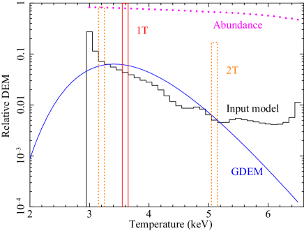
Figure 13: The predicted DEM profile of the Perseus cluster within the FOV of the Hitomi SXS (black histogram) and the corresponding average abundance profile (relative to the proto-solar values of Lodders & Palme 2009; magenta dots). The best-fit isothermal (1T) and two-temperature (2T) models to this DEM are shown with the red and orange histograms, respectively, and the best-fit GDEM model with the blue curve.

We have then integrated these 3D profiles over the line of sight through the projected FOV of the Hitomi SXS for our present observations. We accounted for the different pointing position for Obs 2$+$3 compared to Obs 4 by weighing with the relative exposure times. This way we have obtained the differential emission measure distribution (DEM) within the FOV of the Hitomi SXS. We have binned it in 0.1-keV wide temperature bins. The total emission measure is 1.003$\times$10⁷³ m^-3. Figure 13 shows this distribution (normalized to integral unity) as well as the average abundance for each temperature bin.

We see that the DEM is strongly peaked towards 3 keV, and decreases rapidly towards higher temperatures. This peak corresponds to the coldest gas in the center of the cluster using the Zhuravleva et al. (2014) parameterization (we have assumed that the temperature remains constant for radii smaller than 10 kpc). The DEM then flattens near 5 keV and turns up again above 6.4 keV. This corresponds to the peak in the radial temperature distribution around 250 kpc. The abundance drops almost continuously from 0.82 in the center (at 3 keV) to 0.47 at 6.5 keV.

Thus, we are faced with an extremely skewed DEM distribution over a range of only a factor of two difference in temperature, combined with a monotonous declining abundance pattern that also differs by a factor of two from low to high temperatures. How does this affect our modeling?

We have taken our baseline model, and replaced the main $\sim$4-keV emission component with the 36 temperature components shown in figure 13. The abundances for the different temperature components are the ones shown in figure 13. For simplicity we assume that all elements have the same abundance. All other spectral components (absorption, AGN contribution, etc.) are taken to be exactly the same as in our best-fit baseline model. We then simulated this spectrum with the same exposure time as the observed Hitomi SXS spectrum, and fitted this simulated spectrum the same way as our baseline model.

In order to avoid the overhead of having to simulate many different cases, we have turned the random noise in our simulations off. In this way we get with a single simulation the best-fit parameters (and their uncertainties where needed). A perfect fit would then yield a formal C-statistic of 0.

Table 5: Best-fit parameters of the simulated Perseus spectrum.

Parameter 1T GDEM 2T input $C_{\rm stat}$ 36.37 3.27 2.64 0 $Y_{1}$ ($10^{72}$ m^-3) 9.89 10.11 8.36 10.03 $kT_{1}$ (keV) 3.622 3.529 3.292 3.624 $\sigma_{T}$ — 0.112 — — $Y_{2}$ ($10^{72}$ m^-3) — — 1.69 — $kT_{2}$ (keV) — — 5.12 — Si 0.853 0.787 0.803 0.778 S 0.845 0.787 0.797 0.778 Ar 0.810 0.786 0.784 0.778 Ca 0.778 0.784 0.778 0.778 Cr 0.716 0.763 0.768 0.778 Mn 0.697 0.751 0.777 0.778 Fe 0.725 0.747 0.758 0.778 Ni 0.747 0.763 0.769 0.778

A logarithmic temperature scale $\sigma_{T}$ of the GDEM model.

We first fit this simulated spectrum with our baseline model, where the thermal emission is modeled as a single-temperature component (labeled as 1T). The best-fit reaches a C-statistic value of 36.37, i.e., the isothermal approximation is poorer by 36.37 compared with the true underlying spectrum. This fit (table 5) shows some clear biases. First, the abundance of Si and S, with lines at the low-energy end of the spectrum, are too high by about 10% compared to the input model (the input model does not have a single abundance, but we list the emission-measure weighted abundance for the input model in table 5). On the other hand, the Fe and Ni abundances are too low by 4%. As a result, the Si/Fe ratio is even off by 15%. This bias can be understood from the different temperature dependence of the Si/S lines compared to the Fe/Ni lines. Our model forces these lines to be formed at the same temperature, and the only way to get the line fluxes more or less right is to adjust the abundances.

Interestingly, the Cr and Mn abundances are even lower, by 8–10%. This is due to the fact that the 1T model in the simulation under-predicts the true continuum near the dominant Cr and Mn lines by about 0.3%. As a result, the total simulated flux near these lines can be recovered only by reducing the abundances.

The temperature for this simulated 1T model (3.62 keV) is slightly lower than the temperature for the baseline model (4.05 keV). There may be various reasons for this. First, our spherically symmetric model for the Perseus cluster that we used may be too simplistic. For example, the Chandra intensity map of the Perseus cluster (Zhuravleva et al., 2014, figure 1) shows non-azimuthal fluctuations up to about 50% due to various structures within the Perseus core. Also, there are calibration uncertainties; for instance, for 4-keV plasmas, Schellenberger et al. (2015) shows differences between temperatures derived from Chandra and XMM-Newton that can easily reach 10%. It is not unfeasible that similar differences would exist between the Hitomi SXS temperature scale and that of Chandra. Finally, even with fully deprojected spectra, at the same distance from the cluster center multiple temperature components may co-exist due to different cooling or heating histories of different plasma elements (e.g. Kaastra et al., 2004).

We then fit the simulated spectrum with the Gaussian DEM (GDEM) model, where the DEM is log-normally distributed (the blue curve in figure 13). This model gives a much better description of the simulated spectrum (table 5), with a C-statistic of only 3.27. The corresponding DEM is quite different from the DEM of our input model (the black histogram in figure 13) but because it has the same total emission measure, average temperature and variance as the input DEM distribution, the corresponding spectra are very similar. Note that while the model parameter for the temperature of the GDEM model is 3.53 keV, its emission-measure weighted temperature is 3.59 keV, which is very close to the emission-measure weighted temperature of the input model (3.62 keV) or the 1T fit (3.62 keV). There is still a small bias in the derived abundances, but it is less than 4% for all elements.

The last model we fit to this simulated spectrum is a two-temperature component model (2T) with the abundances of both components tied together. This provides the best-fit (table 5) with a C-statistic value of only 2.64 and and abundance bias smaller than 3%.

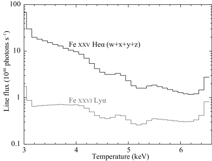
Figure 14: The predicted distribution of the line flux of the main $n=$1–2 transitions of FeXXV and FeXXVI within the Hitomi SXS FOV.

Finally, we have investigated the properties of the strongest lines in the spectrum. Defining line fluxes can be done in two ways: either taking the “pure” line flux, or also including other weak lines that are blended with the line of interest at the spectral resolution of the instrument. We have chosen the latter approach, and included the flux from all lines within $\pm 2$ eV from the line of interest. Figure 14 shows the combined line flux of the four He$\alpha$ transitions w, x, y, and z of FeXXV and the sum of both Ly$\alpha$ lines of FeXXVI. No resonance scattering has been taken into account in these calculations. It is seen that the FeXXV emission is more concentrated towards lower temperatures (the emission-weighted temperature for this ion is 3.69 keV), while FeXXVI has a much flatter distribution (average temperature for this ion is 4.39 keV). Also, the ratio of the sum of the x, y, and z line fluxes to the w line flux changes significantly over this temperature range: from 0.79 at 3 keV to 0.63 at 6.5 keV.

7.4 Multi-temperature fitting of the Hitomi SXS data

Table 6: Parameters of the multi-temperature fits.

Model $C_{\rm stat}$ $Y$ $kT$ $\sigma_{v}$ Abundance (solar) $N_{\rm H,hot}$ ($10^{73}$ m${}^{-3})$ (keV) (km s^-1) Si S Ar Ca Cr Mn Fe Ni ($10^{24}$ m²) Baseline 4926.03 3.73 3.969 156 0.91 0.94 0.83 0.88 0.70 0.74 0.827 0.76 18.8 GDEM 4865.13 3.85 3.830, 0.130 158 0.81 0.84 0.79 0.89 0.78 0.84 0.851 0.79 16.5 2CIE_A 4867.31 2.62, 1.22 3.360, 5.140 157 0.82 0.85 0.78 0.88 0.78 0.84 0.851 0.79 15.6 2CIE_B 4800.50 2.22, 1.53 3.142, 5.166 106, 215 0.81 0.85 0.80 0.90 0.80 0.84 1.041, 0.708 0.80 9.9 3CIE 4790.72 2.22, 1.26 3.578, 5.118 112, 234 0.78 0.84 0.82 0.92 0.78 0.81 0.916, 0.705 0.79 11.9

Expected values for the baseline and multi-temperature models are 4876.
The best-fit parameters of the baseline model adopted from table 1 for comparison.
$\sigma_{T}$ of the GDEM model. It is a common logarithmic temperature scale.
Parameters of the cool and hot ICM components of the 2CIE modeling.
The third component has a temperature of 1.9 keV and best-fit $Y=0.33\times$ $10^{73}$ m^-3. The values of $\sigma_{v}$ and Fe abundance are tied to those of the $\sim$3.5-keV component.

As shown in section 7.3, the central region of the Perseus cluster contains multiple temperature components. To evaluate the impact of the multi-temperature structure on the ICM parameters (e.g., turbulent velocity and abundances) for the real data, we carry out a multi-temperature fit to the Hitomi SXS spectrum. It is known that there is often more than one solution to fit a multi-temperature structure, since models with different combinations of temperatures and abundances might essentially yield a similar spectrum. Exploring these solutions is the focus of T paper. In this paper, we present three basic approximations for the temperature structure, and test them using the Hitomi SXS data.

First we assume that the temperature distribution follows a GDEM form. As shown in section 7.3, the GDEM model provides a proper approximation to the radial temperature profile of the Perseus cluster as derived from Chandra data. In the fit, we adopt the peak temperature, Gaussian width of the DEM, abundances, and turbulent velocity as free parameters, and the remaining components (AGN and resonance scattering) are modeled in the same way as in the baseline model (section 3). The effective-area correction factor (appendix A.2) is also left free, as the continuum of the GDEM model is slightly different from the single-temperature baseline model. The results of the GDEM fits are shown in table 6. The C-statistic improves by 61 compared to the baseline fit. The best-fit central temperature $T$ is 3.83$\pm$0.05 keV, and the Gaussian width $\sigma_{T}=$ 0.13$\pm$0.01, which indicates a significant deviation from isothermality. Note that $\sigma_{T}$ is defined in units of $\log_{10}\,(T)$, hence the value of $\sigma_{T}$ corresponds roughly to 35% of $T$ or 1.3 keV. The GDEM fitting gives lower Si, S, and Ar abundances, a similar Ca abundance, and slightly higher Cr, Mn, Fe, and Ni abundances than the single-temperature run. The abundance changes agree well with the prediction in table 5, indicating that the GDEM results are more close to the real values than the baseline results. The turbulent velocity remains intact in the new fit.

As a second approach, we apply a model with two discrete temperatures. First we assume that the two temperature components have the same set of abundances and turbulent velocity, as well as the same foreground absorption with a column density of 1.38$\times$10²¹ cm^-2. This setting is called 2CIE_A. The other spectral components are inserted in the same way as the baseline model, and the effective area fudge factor is left free in the fitting. As shown in table 6, the C-statistic improves by 59 compared to the baseline fit. The best-fit two temperatures are 3.36$\pm$0.29 keV and 5.14$\pm$0.30 keV, and the abundances and turbulent velocity agree well with those with the GDEM model. The two-temperature fit can be further improved by allowing the Fe abundances and turbulence of the two components to vary freely. This setting is then called 2CIE_B. This fitting improves the C statistic by 126 from the baseline fit.

The fitting result (figure 24 in appendix D) shows positive residuals, about 10–20% of the continuum level, at $\sim$6.47 keV and 6.50 keV in the baseline fit. These residuals remain intact in the fittings with the GDEM or the two-temperature models. Assuming that these features are emitted at the rest-frame of the Perseus cluster, they coincide with the FeXXII and FeXXIII DR lines, at 6.58 keV and 6.61 keV, respectively. As shown in figure 15, these FeXXII and FeXXIII lines are important in low temperature (1–2 keV) plasma. Indeed such a component was recently reported to be associated with the H$\alpha$-bright filaments in the Perseus cluster (Walker et al., 2015). Hence we extend the 2CIE_B model by adding a third CIE component. It becomes the 3CIE model shown in table 6. Since the third component cannot be determined well with the Hitomi SXS spectrum, we tie all of its parameters, except for the temperature and emission measure, to those of the $\sim$3.5-keV component. The best-fit temperature and emission measure are 1.9 keV and 0.33$\times$ 10⁷³ m^-3. The 3CIE model improves the C-statistic by 135 from the baseline fit, although the improvement from the 2CIE_B model is not significant ($\delta C_{\rm stat}=$10). As shown in figure 16, compared to the two-temperature fits, the 3CIE fit provides a better description to the FeXXII and FeXXIII complex at 6.47–6.50 keV.

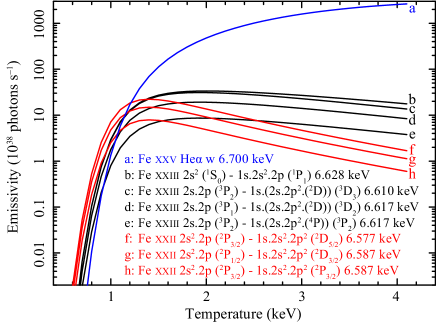
Figure 15: Emissivities of B-like FeXXII and Be-like FeXXIII lines at around rest-frame energies of 6.58 and 6.61 keV, respectively, as a function of temperature. The FeXXV He$\alpha$ w line is plotted as a reference.

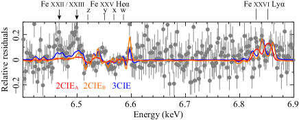
Figure 16: Residuals of the baseline fitting in the Fe band. The red, orange, and blue curves show the changes by the 2CIE_A, 2CIE_B, and 3CIE models, respectively. The black arrows indicate the redshifted energies of FeXXII and FeXXIII DR line complex.

7.5 Helium abundance

Helium is an interesting element. It does not have line transitions in the X-ray band, yet its continuum contribution relative to hydrogen varies by $\sim$5% over the Hitomi SXS band, and therefore our results are affected by the adopted He abundance. It has been discussed that the He abundance in cluster cores may be enhanced by a factor of two or more due to sedimentation (Fabian & Pringle, 1977; Gilfanov & Syunyaev, 1984; Qin & Wu, 2000; Chuzhoy & Nusser, 2003; Ettori & Fabian, 2006; Medvedev et al., 2014; Berlok & Pessah, 2016). However, the magnitude of the effect is hard to predict due to the role of the magnetic topology, plasma instabilities, gas mixing by mergers and turbulence, and the formation of a cool core.

We have tested the effects of an enhanced He abundance on our baseline model by enhancing the He abundance to 1.1 times its original value. The effects are shown in table 1. The main effect is an enhancement of the abundances of all metals by 0.02–0.03.

8 Systematic factors affecting the derived source parameters: spectral components

Besides the (near-)thermal emission from the ICM, the Hitomi SXS spectrum might contain additional spectral components, such as the resonance scattering and the charge exchange between hot and cold matter. Are these components properly modeled in the current atomic codes? We investigate the additional spectral components and calculate the induced uncertainties on the derived properties of the main thermal component.

8.1 Self-absorption by hot gas

Table 7: Strongest absorption lines in the Perseus spectrum.

Line $E$ $\tau_{0}$ $f$ $A$ (keV) ($10^{12}$ s^-1) OVIII Ly$\alpha_{2}$ 0.6535 0.017 0.139 2.6 OVIII Ly$\alpha_{1}$ 0.6537 0.033 0.277 2.6 NeX Ly$\alpha_{2}$ 1.0215 0.010 0.139 6.3 NeX Ly$\alpha_{1}$ 1.0220 0.020 0.277 6.3 MgXII Ly$\alpha_{2}$ 1.4717 0.008 0.139 13 MgXII Ly$\alpha_{1}$ 1.4726 0.016 0.277 13 FeXXIII L$\beta$ 1.1251 0.007 0.256 4.7 FeXXIII L$\beta$ 1.1290 0.011 0.410 7.6 FeXXIV L$\beta$ 1.1627 0.036 0.126 7.4 FeXXIV L$\beta$ 1.1674 0.070 0.243 7.2 FeXXIV L$\gamma$ 1.5505 0.007 0.032 3.3 FeXXIV L$\gamma$ 1.5525 0.013 0.062 3.2 FeXXIV L$\delta$ 1.7304 0.005 0.026 1.7 SiXIV Ly$\alpha_{2}$ 2.0043 0.018 0.139 24 SiXIV Ly$\alpha_{1}$ 2.0061 0.037 0.277 24 SiXIV Ly$\beta_{1}$ 2.3766 0.006 0.053 6.5 SXV He$\alpha$ w 2.4606 0.008 0.767 67 SXVI Ly$\alpha_{2}$ 2.6197 0.016 0.139 41 SXVI Ly$\alpha_{1}$ 2.6227 0.031 0.277 41 ArXVII He$\alpha$ w 3.1398 0.005 0.775 111 ArXVIII Ly$\alpha_{1}$ 3.3230 0.010 0.277 66 CaXIX He$\alpha$ w 3.9023 0.011 0.782 172 CaXX Ly$\alpha_{1}$ 4.1075 0.008 0.277 101 FeXXIV r 6.6533 0.008 0.157 343 FeXXIV q 6.6619 0.025 0.489 471 FeXXV He$\alpha$ w 6.7004 0.338 0.798 518 FeXXV He$\beta_{1}$ 7.8810 0.056 0.156 140 FeXXV He$\delta_{1}$ 8.2955 0.020 0.058 58 FeXXV He$\gamma_{1}$ 8.4874 0.009 0.028 29 FeXXVI Ly$\alpha_{2}$ 6.9517 0.011 0.139 291 FeXXVI Ly$\alpha_{1}$ 6.9732 0.021 0.277 292 NiXXVII He$\alpha$ w 7.8051 0.013 0.683 602

Data based on SPEX v3.03: the rest-frame energy $E$, optical depth $\tau_{0}$ at line center with the best-fit parameters of the baseline model, oscillator strength $f$, and transition probability $A$.
DR satellite transitions of 2s – 1s.2s.2p. See table 10.

As indicated in section 3, we have included a simple model to account for the absorption of photons through the cluster gas itself. In table $*$ ‣ 7 we show the transitions with strong line absorptions in the Hitomi SXS band, including the band that would have been observed if the gate valve would have been opened. The optical depth $\tau_{0}$ at line center is derived by assuming the best-fit baseline parameters of the column density of the hot gas $N_{\rm H,hot}$, abundances, and velocity dispersion $\sigma_{v}$ (table 1). The transitions with optical depths larger than 0.005 are listed. We also list the oscillator strength $f$ and the total transition probability $A$ from the upper level of the line that is used in these calculations (Voigt absorption profiles are being used).

Clearly, the FeXXV resonance line (He$\alpha$ w) has the highest optical depth, but we see significant contributions from the other lines of the same Rydberg series, as well as for other ions of Fe and other elements. Also the optical depth of the FeXXIV lines that block a part of the He-like intercombination line (Mehdipour et al., 2015) is up to 2%, a level that is detectable (for the intercombination line, the statistical uncertainty of the spectrum over one instrumental FWHM of 5 eV is about 3%).

In our baseline model, we have coupled the turbulent velocity, the Doppler velocity and the temperature to the corresponding parameters of the dominant thermal emission component. We have also tested a model where we have decoupled these quantities. We obtain an insignificant improvement of our model (see table 1) with a temperature of 3.8$\pm$0.6 keV for the absorbing gas, a velocity relative to the hot gas of 10$\pm$30 km s^-1, a LOS turbulent velocity dispersion of 191$\pm$35 km s^-1 and a column density of (20.1$\pm$2.2)$\times$10²⁴ m^-2. All these parameters are fully consistent with the parameters of the emission component within the uncertainties of those emission parameters, but obviously we cannot exclude that the properties of the absorbing gas are — on average — within the range indicated by the above uncertainties.

Our model substitutes a simple absorption model for resonance scattering effects. It assumes a common hydrogen-equivalent column density for all the transitions listed in $*$ ‣ 7, ignoring the spatial structure of the ICM. The model also ignores the re-emission process after absorption, which possibly results in lower estimation of optical depths. A more accurate characterization of resonance scattering requires radiative simulations, which will be separately presented in RS paper.

8.2 Charge exchange contributions

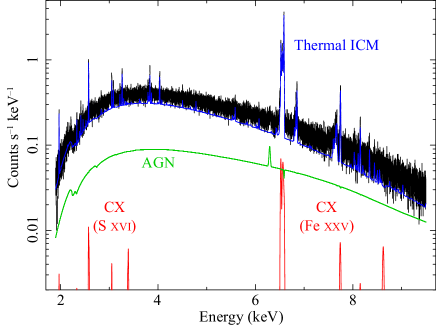
Figure 17: The best-fit result with the CX emission. Each X-ray emission component is shown: thermal ICM in blue, AGN in green, and CX in red.

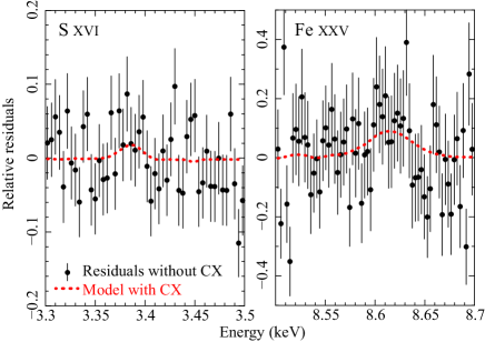
Figure 18: Residuals of the baseline fitting in the SXVI 3.2–3.6 keV (left) and FeXXV 8.3–8.8 keV (right) bands. The red curve in each panel shows the model change by including the CX component.

Charge exchange (CX) happens when a neutral atom collides with a sufficiently charged ion, which recombines with the electron(s) captured from the atom. The product ion often has a highly excited state with large principal quantum number $n$, and thereafter, the decay of the excited electron(s) will fill the inner-shell vacancies through line emission. Therefore, the most characteristic features of the CX emission in X-rays are the transitions from high-$n$ shells to the ground, which are much stronger than those in the CIE case. The CX spectrum also exhibits higher Ly$\beta$-to-Ly$\alpha$ and forbidden-to-resonance (z-to-w) ratios, although these features can be achieved by other atomic processes (Gu et al., 2016b).

In this section we examine the CX contributions to the ICM emission of the Perseus cluster with the Hitomi SXS spectrum. The CX component adopted here is described in Gu et al. (2016a). It uses velocity-dependent, $nlS$- (He-like) or $n$- (H-like) resolved reaction cross sections, based primarily on the multi-channel Landau-Zener calculations (Mullen et al., 2016). The low-energy weight function (equation 4 of Gu et al., 2016a) is applied to the H-like data in which the $l$-distribution cannot be obtained by the Landau-Zener calculations. For the Li-like and Be-like sequences, it includes velocity- and $nl$-resolved cross sections which are derived from an empirical scaling relation presented in Gu et al. (2016a). In this model, only the atomic component of the cold gas is considered, although in reality the molecular gas also contributes. The collision velocity is set to 200 km s^-1 (Conselice et al., 2001), and the ionization temperature and abundances of the CX ions are fixed to the best-fit values of the ICM thermal component. As shown in table 1, a new baseline run including the CX component results in a minor C-statistic improvement ($\delta C_{\rm stat}=$13).

The fitting prefers that the CX lines are more broadened than the CIE lines, with a turbulent velocity $v_{\rm mic}\gtrsim$600 km s^-1 (or $\sigma_{v}\gtrsim$400 km s^-1). Since the actual line profile cannot be determined by the current data, we fix the turbulent velocity of the CX component at $v_{\rm mic}=$ 800 km s^-1, corresponding to $\sigma_{v}$ of 566 km s^-1 which is the upper limit of the neutral atomic line width of the molecular cloud near NGC 1275 as reported in, e.g., Salomé et al. (2011). The large line width might be caused by a combined effect: it can be partially contributed by the kinematics of the neutral cloud and the ICM, and partially from the atomic uncertainty of the capture state (Gu et al., 2016a), as the CX lines from $n\geq$10 levels are often blended. Changing the turbulent velocity to a larger value (e.g, 1000 km s^-1) has a negligible effect on the fitting.

As shown in figures 17 and 18, the CX model predicts that the most promising high-$n$ transitions are seen in the SXVI band, which has been reported by Hitomi Collaboration et al. (2017a), as well as the FeXXV band. The CX lines contribute to $\sim$1% of the continuum for SXVI at $\sim$3.4 keV, and $\sim$3% for FeXXV at $\sim$8.6 keV. To measure the statistical uncertainties, we replace the CX model with two Gaussian lines at the energies of the SXVI and FeXXV high-$n$ transitions. The Gaussian FWHM is set free for each line. The SXVI and FeXXV CX lines have 1.6-$\sigma$ and 2.4-$\sigma$ significances, respectively. However, it is premature to claim the detection of CX with the current data, since the uncertainty from the effective area/gain calibration is large and energy dependent, as discussed by Hitomi Collaboration et al. (2017a). For the remaining ions, the high-$n$ transitions are negligible, either due to the low abundances, or blending with strong thermal lines.

As shown in table 1, inclusion of the CX component has minor effects on the ICM temperature, emission measure, and turbulent velocity. The Fe and Si abundances are reduced by $\approx$ 5% and 2%, respectively, and the S, Cr, Mn, and Ni are affected by 1–3%. Since the CX emission has a larger forbidden-to-resonance (z-to-w) ratio than the thermal emission, the equivalent $N_{\rm H,hot}$ for the possible resonance scattering is reduced by about 7%. The effect on the resonance scattering study will be further discussed in RS paper.

8.3 AGN contribution

To assess the uncertainty from the AGN flux, here we first consider an extreme condition: the central AGN is quite dim and its power-law emission is negligible. As shown in table 1, the non-AGN run gives a much worse fit ($\delta C_{\rm stat}=$ 625) than the original baseline fit, and the best-fit temperature shifts by 0.5 keV. The abundances are systematically lower by 0.01–0.21 solar.

Next we examine a more realistic case for possible systematic uncertainty related to the detailed AGN modeling. The AGN spectrum in the baseline model was established in the early study for AGN paper with the PSF photometry. The technique is essentially unchanged in the final analysis but the energy band is extended up to 20 keV with the sxsextend tool. The broader-band spectrum requires a slightly flatter photon index and a $\approx$20% lower flux in 2–10 keV (see AGN paper for details). Another notable update is the RMF type, which has been changed from the large size (also used in our baseline model) to the extra-large size to include electron-loss continuum. As we examine the effect of using different types of RMF separately (section C.2), we use the new AGN model derived in the same method as in AGN paper but with the large-size RMF for a straightforward comparison to the baseline model. Therefore, slightly different parameter values from AGN paper are adopted in our test: the photon index of 1.85 and the 2–10-keV flux of 2.9$\times$10^-14 W m^-2 (private communication with H. Noda and Y. Fukazawa, 2017).

The new AGN model run gives a slightly poorer fit ($\delta C_{\rm stat}=$ 11) than the original baseline model. The lower AGN flux requires a significant rise of the ICM continuum by 6%, which results in 3–4% lower abundances. The change in the ICM gas temperature becomes insignificant, unlike the no-AGN case.

9 Systematic factors affecting the derived source parameters: fitting techniques

In this section we discuss the effects of applying different fitting techniques on the derived parameters of the baseline model.

9.1 Comparison of $\chi^{2}$-statistics versus the default C-statistics

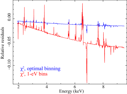
Figure 19: Relative differences between a $\chi^{2}$ fit and a C-statistic fit (blue curve) for the baseline model. The red curve shows the same but with 1 eV bins instead of optimal binning.

It is well known that the use of $\chi^{2}$-statistics in spectral fitting can give bias in the estimated parameters (e.g. Nousek & Shue, 1989; Mighell, 1999). The proper way to resolve this is to use C-statistics (Cash, 1979), and we have used that for our baseline model. We use the modification of C-statistic as proposed by Castor (see the Xspec manual, Arnaud 1996). This modification is the standard in the Xspec and SPEX packages. Our present Hitomi SXS spectrum offers an excellent opportunity to demonstrate the bias that one gets when using $\chi^{2}$-statistics. We have taken the baseline model and replaced the C-statistic with the $\chi^{2}$ statistic in the spectral fit. The best-fit model has $\chi^{2}=$6192 for 5790 degrees of freedom. The value of the C-statistic that corresponds to this $\chi^{2}$-optimized fit is 88 higher than for the baseline model. We show the relative difference between both models in figure 19.

It is seen that the continuum for the $\chi^{2}$ fits is about 1% lower than for the baseline model, while some of the stronger emission lines have similar fluxes for both cases. This 1% bias is caused by the well-known effect that $\chi^{2}$ fits tend to give lower fluxes by giving relatively more weight to the data points that by chance have a flux below the expected value than to the data points that have a flux above it. Our present spectrum has typically 100 counts in most continuum bins, and according to Mighell (1999) this would give a bias of about 1 count, in remarkable good agreement with our findings here. Note that for typically 100 counts per bin, the Poissonian error bars are about 10 counts, hence much larger than the differences between the models. This shows that biased fits are easily overlooked if plotted at full resolution. Only rebinning the best-fit drastically (with a factor of at least a hundred or so) would show the bias.

The bias becomes even stronger if in addition to using $\chi^{2}$-statistics we drop the optimal binning and use 1-eV bins (see the red curve in figure 19). In addition to a lower flux, there is now also a significant bias in the temperature, leading to a different overall slope of the spectrum. The bias is even 6% at the highest energies.

9.2 Optimal binning versus other binning

We have also tested how our results depend on the adopted bin size. When we use C-statistics, we find no difference at all for the parameters shown in table 1 when comparing our optimal binning with a uniform binning of 1 eV. This is easily understood by noting that our optimal binning already gives a bin size of 1–2 eV for all bins (see appendix A.3), and that it is more the order of magnitude of the bins rather than the precise bin size that matters for the sensitivity of statistical tests (Kaastra & Bleeker, 2016, see figure C3).

Note that when $\chi^{2}$ is being used, binning is important, but as we demonstrate in section 9.1, the use of $\chi^{2}$-statistics should be avoided.

9.3 Local versus global fit

Astrophysical spectroscopic analysis in the radio through ultraviolet bands often relies upon precise measurements of selected, strong emission lines (e.g., HI 21 cm, FeII 1.257 $\mu$m, and [OIII] 5007 Å) whose atomic and diagnostic properties are well-understood. This can also be done with X-ray spectroscopy (Hitomi Collaboration et al., 2016), but both the physics of X-ray–emitting plasmas and the availability of high-resolution spectrometers create significant challenges.

The Hitomi SXS spectrum of Perseus presents a clear combination of emission lines with a continuum, implying it can be completely understood via fits with the sum of a simple continuum plus a series of Gaussian emission lines, with astrophysical parameters derived from positions, widths, and flux ratios of the Gaussian parameters. An advantage of this approach is that it requires a relatively small amount of reliable atomic data, enabling the use of experimentally-verified and theoretically-understood features. For example, the ratio of the line intensity of the Ly$\alpha$ line to its resolved DR satellites depends critically on the electron temperature; advanced line diagnostics using multiple DR satellite lines even test whether the underlying plasma is in thermal equilibrium (Gabriel & Phillips, 1979; Kaastra et al., 2009).

Although elegant, and without doubt useful to obtain an approximate description, this approach will miss details resulting from a self-consistent fit of the full spectrum. Three key problems occur with X-ray spectral analysis via purely local line fits:

1. Unlike other spectral bands, the line and continuum emission arise from the same plasma. Therefore, simplifying the continuum to a spline fit or even bremsstrahlung emission independent of the line components ensures the resulting analysis will miss features. The X-ray continuum, even in strict collisional ionization equilibrium, contains significant contributions from radiative recombination continua and two photon emission (see e.g., figure 8 in Kaastra et al., 2008). While these components can be included in the fit, e.g., the APEC No-Line model used in Plucinsky et al. (2017), separating line from continuum emission makes finding a self-consistent model all but impossible.

2. X-ray spectrometers, even the SXS, have only limited resolution, while the X-ray bandpass has a plethora of strong lines, making line blending an ongoing problem. Table E in appendix E shows several instances of lines from different elements separated by less than the instrumental resolution. Worse, the narrow bandpasses of oft-used diagnostic lines such as the He${\alpha}$ complex includes a multitude of DR satellite lines together with the strong “triplet” (actually a quartet) lines. Many of the lines have multiple excitation channels all of which must be known in order to fit the complex reliably. This is especially true of the forbidden line (z), as discussed earlier. For the SXS spectrum, Gaussian lines were used to determine the turbulent motion (Hitomi Collaboration et al., 2016), but a local form of the global fit is required to extract the maximum amount of information even from a relatively small bandwidth. At a minimum, when applying line ratio diagnostics it must be clear both in the model and the data whether these contaminants have been taken into account.

3. Few, if any, sources in the Universe will be in perfect equilibrium, either collisional or photo-ionized. The present spectrum of the Perseus cluster is a good example of such complexities. While dominated by a 4-keV temperature component, the possibility of multi-temperature cannot be eliminated based on the data (section 7.4), and is certainly expected theoretically. Depending upon their excitation mechanism, each emission line will be affected differently by these effects, rendering the use of just one or two diagnostic ratios precise but quite inaccurate. Using many lines, including upper limits to non-detections, will avoid this problem, but at some point the distinction between a many-line vs a global fit will become blurred.

Despite the above issues, line ratios may be preferred over global fits when the source spectrum is either too complex to be fully understood, or when calibration uncertainties dominate the broad-band spectra. Of course, the accuracy of the physical parameters derived from global fits also relies upon complete and accurate atomic databases. In the case of completeness, global models contain potentially millions of atomic transitions, most of which have not been experimentally verified. While “spot” checks do exist, in most cases the accuracy of the data is not well known, i.e., estimates of uncertainties are determined by comparing results from different theoretical calculations, or by using uncertainties from portions where experimental results do exist.

In our case, we have shown that the calibration and completeness of the spectral models is not perfect but good enough to yield a very good description of the Perseus spectrum. Ultimately, local and global fits must be used in a complementary way. The broad bandwidth coupled with the high spectral resolution of the SXS makes it possible to take advantage of the strengths of both methods, improving the reliability of the derived physical parameters of the source.

10 An improved model

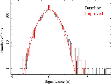
Figure 20: Diagrams showing the significance of an additional line model, on the top of the best-fit baseline model (black) and improved model (red), with the central energy moving across the entire band. The red curve shows a $\sigma=$1 Gaussian function that fits the diagram of the improved model.

To fit the Perseus spectrum, we introduced a baseline model (section 3) which mainly consists of a $\sim$4-keV CIE plasma and an AGN component. Obviously the baseline model is merely a simple approximation (section 7.4), even though it already achieves a satisfactory fit based on the current Hitomi SXS data. Throughout the paper, we have tested a variety of plasma codes, atomic data calculations, plasma and astrophysical modelings, additional spectral components, and instrumental effects, and compared them with the original baseline fit. By properly incorporating some of the atomic and astrophysical effects into the baseline model, we are able to achieve a more advanced physical model of the Perseus spectrum.

We construct an improved model as follows. Following the baseline model, SPEX version 3.03 is used, the abundance standard are the Lodders & Palme (2009) proto-solar values, and the ionization balance is set to Urdampilleta et al. (2017). The thermal emission is modeled now by the sum of three CIE components, with temperatures of about 2 keV, 3.5 keV and 5 keV (section 7.4). The three-temperature model is chosen since it gives the best fit of all multi-temperature modelings (table 6). The three components have the same Si, S, Ar, Ca, Cr, Mn, and Ni abundances, while the Fe abundance and turbulent velocity are left free for the 3.5-keV and 5-keV components. For the 2-keV component, the Fe abundance and turbulent velocity are tied to those of the 3.5-keV component (section 7.4). The AGN contribution, resonance scattering, and the Galactic absorption components are added in the same way as for the baseline model. The possible CX component (section 8.2) is included in the improved model. Following section 6.1, the Voigt function is used to describe the line profiles. We re-fit the effective area correction factor in the same way as described in appendix A.2, and show the best-fit model in figure 22 (a).

The improved model achieves a so-far best C-statistics, 4779 for an expected value of 4876$\pm$99, which is significantly better than the baseline fit (C-statistics $=$ 4926). The best-fit model is plotted in appendix D (figures 23–25), and the stacked residual diagram is shown in figure 20. The residual diagram is calculated by adding a line component, with the central energy moving from 1.9 keV to 9.5 keV with a step of 3 eV, on the best-fit baseline and improved models. Compared to the baseline run, the residuals at $>$2$\sigma$ are greatly suppressed by the improved fit, and the diagram follows well the expected Gaussian distribution. As shown in table 1, the new model essentially reproduces the best-fit results of the three-temperature model (section 7.4). The best-fit temperatures are 1.92$\pm$0.21 keV, 3.61$\pm$0.33 keV, and 5.43$\pm$0.38 keV for the three components. Note that the values are sensitive to the details of the spectral modeling as well as the calibration of the instrumental response (see T paper for further details). All the Si, S, Ar, Cr, Mn, and Ni abundances become roughly 0.8 solar, which are much more uniform than the baseline results. The Ca abundance remains to be about 0.9 solar. The best-fit Fe abundances are 0.91$\pm$0.05 solar and 0.64$\pm$0.05 solar for the 3.5-keV and 5-keV components, respectively. The turbulent velocities become $\sigma_{v}=$ 117$\pm$11 km s^-1 for the 3.5-keV component and $\sigma_{v}=$ 223$\pm$27 km s^-1 for the 5-keV component. This may suggest that the cooler ICM tends to have a lower level of turbulence than the hotter one, but the results depend on the assumed temperature structure and are sensitive to the continuum modeling including the effective area calibration. The further details are discussed in V paper. Moreover, the improved model gives a self-absorption column density of $($1.05$\pm$0.15$)\times$10²⁵ m^-2. The column density of FeXXV is thus $($2.18$\pm$0.23$)\times$10²⁰ m^-2, in good agreement with the value that we derive from the simulated spectra in section 7.3 (4.02$\times$10²⁰ m^-2 for the semi-column of a line through the core; 2.64$\times$10²⁰ m^-2 for the semi-column averaged over the Hitomi SXS FOV). Details on the derived resonance scattering are discussed in RS paper.

11 Discussion

11.1 Important factors

We have shown in this paper the dependencies of several astrophysically interesting parameters, mainly focusing on the plasma modeling, i.e., plasma codes and atomic databases. We have also investigated the dependencies on astrophysical modeling as well as spectral fitting techniques. For a proper astrophysical modeling of the present Perseus cluster spectra, as presented here but in greater detail discussed in a set of other papers (Hitomi Collaboration et al. 2016, 2017a, Z, T, RS, V, and AGN papers), it is crucial to understand the possible systematic biases on the derived parameters. Table 1 provides a comprehensive list of the estimated biases, which enables us to inter-compare various aspects of systematic uncertainty. The effects of some of the plasma modeling factors are comparable to or even larger than the statistical or instrumental uncertainty (appendix C). Because this is the only high-quality high-resolution X-ray spectrum of a spatially extended thermal X-ray source up to now, it is also important for the preparation of future X-ray missions, in the sense that priorities in calibration, astrophysical modeling, or data analysis can be set.

11.1.1 Emission measure

The emission measure $Y$ of the cluster ICM is a good representative of the absolute flux of the hot cluster gas. First, it is clear that we need to use the latest aharfgen to obtain an accurate emission measure. Although the emission measures are uniformly underestimated by 20% for the other cases with the older software, hereafter we ignore the difference and compare the relative values to find out which parameter affects $Y$.

The main contributor to the systematic uncertainty on $Y$ is the adopted flux of the central AGN. Ignoring the AGN completely would give a 20% higher emission measure as well as 12% higher temperature for the hot gas. In fact, the AGN contribution affects almost all parameters of the hot cluster gas. Because we are not completely ignorant about the AGN flux, the true uncertainties are smaller than described above. One example of more realistic estimation is the difference due to updating the AGN model with the broader-band spectroscopy, which gives a 6% higher emission measure.

Other important factors for $Y$ are the effective area correction (up to 4%), the ionization balance (3%), and the assumption of isothermality ($\sigma_{T}$ free, 3%). The differences between the plasma codes, for which we consider here SPEX version 3.03 and AtomDB version 3.0.8 (SPEX and AtomDB briefly hereafter) to be the most sophisticated, are not very important for the emission measure: differences are less than 1%.

11.1.2 Temperature

Ignoring from now on the AGN contribution uncertainty, the most important factor affecting the temperature of the dominant 4-keV component is the fitting techniques. Using unbinned spectra and $\chi^{2}$ statistics biases the temperature by 5%. Forcing isothermality (i.e., putting $\sigma_{T}$ to be zero) gives 3.5% bias. Using the official effective area correction based on the on-ground calibration instead of the additional effective area correction using a thinner Be-filter and knak gives 3% bias. Both plasma codes (SPEX and AtomDB) agree relatively well in their derived temperature (better than 2%).

11.1.3 Turbulent velocity

While the temperature agreement between the plasma codes is good, they result in a 10% difference in the derived amount of turbulence in the plasma. This uncertainty is almost as large as the uncertainty introduced by ignoring completely the resonance scattering or ignoring the position-dependent bulk velocity field (both 9%).

11.1.4 Cluster velocity

This bulk velocity field obviously also affects the derived velocity centroid of the cluster (23 km s^-1). Obviously the gain correction is also important (14 km s^-1). Finally, the use of SPEX or AtomDB also results in a difference of 6 km s^-1.

11.1.5 Resonance scattering

The plasma codes result in an even bigger difference of 40% in the derived column density of the resonantly scattering plasma, six times larger than the statistical uncertainty on this quantity. This relatively large difference is likely associated to the systematic uncertainties in the line emissivities, because in the comparison we use the same resonance scattering model (the SPEX hot model). However, also precise modeling of the temperature structure (see our improved model) is important: this can also produce a difference of 35%.

11.1.6 Abundances

Finally, we discuss here the uncertainties on the abundances. Most striking is the difference in the Fe abundance associated to the plasma code: AtomDB gives a 16% lower abundance than SPEX. This is 17 times higher than the small statistical uncertainty on the Fe abundance. The differences can be attributed mostly to differences in the adopted collisional excitation and DR rates of the strongest spectral lines (sections 5.1 and 5.3). Other factors affecting the Fe abundance are the inclusion of resonance scattering (11%) and CX (5%). On the other hand, the Ni abundance is almost bias-free between the latest SPEX and APEC/AtomDB (at least within its 7% statistical uncertainty; however the bias between SPEX versions 2 and 3 is still significant. See also Z paper). This is not the case for other elements. The Si and S abundance can be biased by 6–14% depending on each of the following four factors: the plasma code, the isothermality assumption, the gain correction and the fitting method ($\chi^{2}$ fitting on unbinned data). For Ar and Ca the main systematic uncertainties are associated to the plasma model (6–8%). Finally, for Cr and Mn both the isothermality assumption and the fitting method are the main sources of systematic uncertainty.

11.1.7 Implications to other observations

So far we have reviewed the state-of-the-art knowledge, mostly on the K-shell transitions, for modeling the hot (several keV) tenuous plasma in collisional ionization equilibrium. We caution that the atomic uncertainties derived from the Perseus data cannot simply be copied to observations of other sources, as the accuracy of atomic data depends strongly on the types of transitions (tables 2 and 3), as well as on the plasma conditions, such as electron temperature (figures 2 and 4) and ion charge states (figures 6 and 7). For instance, X-ray emission from a stellar corona (or an elliptical galaxy) is dominated by transitions in the Fe-L complex, which are known to be computationally more intricate than those in the Fe-K (e.g., Bernitt et al. 2012), and hence less accurate (e.g., de Plaa et al. 2012).

A more important issue is to discuss the atomic uncertainties by the science cases. The doppler measurement of line-of-sight velocities would be subject to the reference-wavelength accuracy of the dominant transitions except for the cases with large bulk velocities for example in young supernova remnants (SNRs). The precise characterization of turbulence velocity structures, i.e., search for non-Gaussianity, would primarily be limited by the accuracy of atomic and astrophysical modeling of the RS effect. This could be avoided by making use of local fittings of optically thin emission lines, and in this case relative line energies and emissivities of satellite lines as well as the calibration of the line spread function are the dominant source of uncertainty. The detection of a small departure from CIE (e.g., for merger clusters; Inoue et al. 2016) would mainly be limited by the uncertainties in the charge-state distribution calculation and thus ionization and recombination rates adopted therein (section 7.2). Revealing detailed time evolution of NEI plasma by measuring the charge-state distribution (e.g., for recombining plasma in SNRs; Sawada & Koyama 2012) would require an even higher level of accuracy for these transition rates including multiple ionization due to inner-shell processes followed by Auger ejections. The elemental abundance measurement is affected mostly by the errors of the line excitations and branching ratios for individual transitions including those for the satellite lines, although only the error of the total emissivity of a line complex (e.g., He$\alpha$) would matter for a system with a large intrinsic line broadening ($\sim$100 eV) like young SNRs where the ion temperature is considerably high ($\sim$MeV).

The atomic uncertainty for each science case can be evaluated by the Monte-Carlo approach introduced in section 5.1.2. Ultimately, the atomic error calculation should be implemented as a standard analysis procedure in the spectral modeling packages. This would require substantial work in the code development by assessing the accuracy of detailed atomic data.

11.2 Atomic data needs

As shown throughout this paper, the reliability of a spectral modeling package lies not only in the accuracy and completeness of its atomic data, but also in its ability to properly synthesize the atomic data as a function of physical parameters, i.e., the plasma conditions, such as temperature and density. Synthesizing the data is tedious and computationally taxing owing to the fact that the databases employed are large, containing millions of data points, including transition energies, excitation and ionization cross sections, resonant (multi-electronic) and non-resonant (radiative) recombination cross sections, and non-thermal processes, such as CX recombination. Different models use atomic databases of varying levels of completeness and accuracy as well as different synthesis methods in their calculations. Estimates of a model’s accuracy is often given by comparison to other models. However, a true measure of a model’s accuracy can only be determined by comparing to laboratory benchmark measurements.

Benchmark measurements, generally, come in two forms: as isolated experiments where a single ionic species or atomic process is studied, or as integrated experiments, where emission or absorption is measured from several simultaneous ions and atomic processes as a function of temperature or density. Isolated experiments include those conducted at electron beam ion traps, advanced light sources, or storage rings. Integrated experiments include experiments using, for example, tokamaks or laser-produced plasmas. Isolated experiments generally test portions of atomic databases, and integrated experiments test synthesis models. Examples of isolated experiments include measurements of absolute electron-impact excitation cross sections as a function of electron energy, transition energies, natural line widths, and oscillator strengths (Beiersdorfer et al., 1992; Brown et al., 2006; Rudolph et al., 2013). Examples of integrated experiments include the spectral signature of the He$\alpha$ complex as a function of electron temperature (Bitter et al., 2008; Gu et al., 2012; Rosen et al., 2014; Rice et al., 2015), or full Fe-K and Fe-L shell spectral signatures as a function of temperature and density.

Providing laboratory benchmarks for the atomic database in all physical regimes for all astrophysically relevant ions is not tractable. Hence, models are tested by comparing to measurements where available. Typically, models agree with measurements at the 10–20% level in the cases of excitation and ionization processes. Transition energies, however, are of much higher accuracy. In the case of H- and He-like ions, measurement of the transition energies have tested theory at the level of a few to a few tens of parts per million (Johnson & Soff, 1985; Beiersdorfer, 2009; Beiersdorfer & Brown, 2015). In the case of ions with more bound electrons, i.e., L-shell ions, the accuracy of the models is not as well known, as experimental benchmarks are more sparse and agreement with theory varies.

The inability of the standard X-ray astrophysics models to accurately fit a significant fraction of the lines in the SXS Perseus spectrum (Hitomi Collaboration et al., 2016) not only uncovered some of the limits of SPEX and APEC, it also showed the limits of the high-accuracy laboratory measurements. For example, laboratory measurements of relative line intensities in the Fe He$\alpha$ complex, in particular the strength of the forbidden line (z), still introduce a limit to our ability to take full advantage of the line complex’s diagnostic power. The high-quality SXS Perseus spectrum provides the impetus for more complete and higher accuracy calculations and systematic measurements of all the processes involved in exciting, not only the forbidden line (z), but all of the lines found in the He$\alpha$ complex, and not only for He-like Fe XXV, but also for other astrophysically relevant He-like ions. Measurements such as these will be paramount to interpreting high-resolution spectra to be returned by the future high-resolution X-ray spectroscopy missions (see section 11.3). Largely driven by their large bandwidths, high energy resolution, and large collecting areas, high accuracy measurements of a plethora of atomic parameters will be required.

While providing a complete list of required measurements is beyond the scope of this paper, a few necessary measurements, in addition to the studies of He$\alpha$, should be mentioned. For example, a more complete study of the excitation cross sections and spectral signatures of CX recombination should be completed. Many CX studies have been completed, however, at present, theory has not matured to a point of consistently predicting experimental results, and hence, the diagnostic capability of CX emission is limited. Absolute cross-section measurements for electron-impact excitation followed by cascades, especially in the case of high-$n$ transitions, with accuracies on the order of 5–10%, should also be a high priority as they determine the line strengths, and in turn, relative ion abundances (ionic fractions) and elemental abundances from a variety of celestial sources. High-accuracy measurements of DR-resonance strengths and of ionization cross sections should also be pursued. Similar laboratory measurements of photo-excitation and ionization processes should also be conducted, as these are the basis for determining column densities and scattering effects (RS paper).

One of the most sought after and challenging integrated laboratory experiments is an accurate measurement of the ion charge balance as a function of electron temperature and density. This is a universal goal throughout plasma physics, spanning nearly all temperature and density regimes. Integrated experiments such as these are challenging because it is hard to know to high accuracy what the systematics are of the source plasma, i.e., it is often hard to quantify or experimentally discount gradient and non-uniformity effects. Regardless of these challenges, integrated experiments where the plasma parameters have been independently well diagnosed have been successfully conducted (Rosen et al., 2014).

11.3 Prospects for XARM, Athena and other missions

The Hitomi SXS observation of Perseus, with its high-resolution spectrum in the 1.9–9.5 keV band, showed both the strengths and weaknesses of existing plasma codes. Pre-launch versions of both the SPEX and AtomDB codes provided generally plausible fits to the observation, matching the continuum and many of the strong lines well. While neither fit was formally statistically acceptable (see table 1), the two codes agreed (to within $\pm$0.3 keV) on the best-fit temperature, and to within $\pm$0.2 on elemental abundances. At CCD resolution, these discrepancies could easily be understood as calibration issues or inadequacies of the collisional isothermal model; only at the resolution of the SXS were the clear problems with both codes apparent. As described above, many of these disagreements could be addressed by updating wavelengths and cross sections for a few weaker lines and by fixing minor code bugs. As a result, both SPEX and AtomDB are in close agreement about the emission from a 4-keV collisional plasma in 1.9–9.5 keV.

That an SXS observation was required to discover and address these problems may seem odd, as gratings on both Chandra and XMM-Newton have provided high-resolution X-ray spectra of point sources since 1999. Unfortunately, most X-ray point sources have intrinsically complex and variable spectra; stellar coronae include plasmas with a broad range of temperatures, while any model of the absorbed photo-ionized spectra of X-ray binaries and AGN must include a range of different geometries and source spectra. The only truly simple point-source spectra are isolated neutron stars or white dwarfs, which have no features in the X-ray band and are therefore used as calibration sources. As a result, few grating observations could be used to test details of the plasma models beyond the strong lines, since any differences in weaker features could reasonably be due to issues in the source model and not the code.

Substantial work remains, therefore, to ensure that current plasma codes will be ready to face the challenges of data from the X-ray Astronomy Recovery Mission (XARM), ESA’s Athena mission, and proposed missions such as the Arcus grating spectrometer or the Lynx observatory. These missions will have resolutions similar to or better than the Hitomi SXS, and will observe a large range of sources, including collisional plasmas with temperatures between 10⁴–10⁹ K and photo-ionized plasmas with a similarly broad range of source flux, either in ionization equilibrium or non-equilibrium. These missions will cover a bandpass of $\approx$0.1–10 keV, a range that includes strong lines from Fe L-shell ions (FeXVII–FeXXIV) as well as M-shell lines from many abundant elements.

The Hitomi SXS data have shown that accurate atomic models are just as important as calibration. Preparing for these missions will require a multifaceted approach of plasma-code testing, theoretical calculations, and laboratory measurements. The process will begin with systematic testing of existing atomic models against (1) each other to determine where discrepancies exist, (2) laboratory measurements from electron beam ion traps and synchrotrons, and (3) deep targeted observations with existing observatories. When areas of unresolvable disagreement are identified, new theoretical calculations may be required or targeted laboratory measurements made. The plasma-code community has already begun this work, starting with a set of agreed-upon standard tests developed at a meeting at the Lorentz Center. However, a consistent and continuous effort will be required to ensure that the community is ready for this next generation of high-resolution X-ray spectra.

Author contributions

M. Sawada, L. Gu, and J. Kaastra led this study and wrote the final manuscript along with R. K. Smith, A. R. Foster, G. V. Brown, H. Odaka, H. Akamatsu, and T. Hayashi. L. Gu, J. Kaastra, and M. Sawada performed the final SXS data reduction and spectral analysis. A. R. Foster and R. K. Smith, A. J. J. Raassen, and G. V. Brown provided inputs on APEC/AtomDB, FAC calculations, and discussion on the atomic data needs, respectively. L. Gu performed the Monte-Carlo simulations for the evaluations of the systematics of the atomic data. C. A. Kilbourne contributed to the estimation of the SXS energy-scale uncertainty. R. K. Smith contributed to the discussion on the future prospects. N. Ota and M. A. Leutenegger respectively contributed to the estimations of the atomic data and plasma modeling systematics. H. Akamatsu and S. Nakashima contributed to the systematics on astrophysical models. K. Sato, H. Noda, and Y. Fukazawa contributed to the estimations of non-ICM components. S. Nakashima and M. Tsujimoto provided the data for the evaluations of the effective-area systematics. T. Hayashi confirmed the in-orbit calibration and performance of the X-ray mirrors of the SXS. N. Hell, M. Tsujimoto, and R. F. Mushotzky contributed valuable comments on the manuscript.

The science goals of Hitomi were discussed and developed over more than 10 years by the ASTRO-H Science Working Group, all members of which are authors of this manuscript. All the instruments were prepared by joint efforts of the team. The manuscript was subject to an internal collaboration-wide review process. All authors reviewed and approved the final version of the manuscript.

We acknowledge reviewer Paul Bryans for the constructive comments and advices. We thank the support from the JSPS Core-to-Core Program. We acknowledge all the JAXA members who have contributed to the ASTRO-H (Hitomi) project. All U.S. members gratefully acknowledge support through the NASA Science Mission Directorate. Stanford and SLAC members acknowledge support via DoE contract to SLAC National Accelerator Laboratory DE-AC3-76SF00515. Part of this work was performed under the auspices of the U.S. DoE by LLNL under Contract DE-AC52-07NA27344. Support from the European Space Agency is gratefully acknowledged. French members acknowledge support from CNES, the Centre National d’Études Spatiales. SRON is supported by NWO, the Netherlands Organization for Scientific Research. Swiss team acknowledges support of the Swiss Secretariat for Education, Research and Innovation (SERI). The Canadian Space Agency is acknowledged for the support of Canadian members. We acknowledge support from JSPS/MEXT KAKENHI grant numbers JP15H00773, JP15H00785, JP15H02070, JP15H02090, JP15H03639, JP15H03641, JP15H03642, JP15H05438, JP15H06896, JP15J02737, JP15K05107, JP15K17610, JP15K17657, JP16H00949, JP16H03983, JP16H06342, JP16J00548, JP16J02333, JP16K05295, JP16K05296, JP16K05296, JP16K05296, JP16K05300, JP16K05309, JP16K13787, JP16K17667, JP16K17672, JP16K17673, JP21659292, JP23340055, JP23340071, JP23540280, JP24105007, JP24244014, JP24540232, JP25105516, JP25109004, JP25247028, JP25287042, JP25400236, JP25800119, JP26109506, JP26220703, JP26400228, JP26610047, and JP26800102. The following NASA grants are acknowledged: NNX15AC76G, NNX15AE16G, NNX15AK71G, NNX15AU54G, NNX15AW94G, and NNG15PP48P to Eureka Scientific. H. Akamatsu acknowledges support of NWO via Veni grant. C. Done acknowledges STFC funding under grant ST/L00075X/1. A. Fabian and C. Pinto acknowledge ERC Advanced Grant 340442. P. Gandhi acknowledges JAXA International Top Young Fellowship and UK Science and Technology Funding Council (STFC) grant ST/J003697/2. Y. Ichinohe, K. Nobukawa, and H. Seta are supported by the Research Fellow of JSPS for Young Scientists. N. Kawai is supported by the Grant-in-Aid for Scientific Research on Innovative Areas “New Developments in Astrophysics Through Multi-Messenger Observations of Gravitational Wave Sources”. S. Kitamoto is partially supported by the MEXT Supported Program for the Strategic Research Foundation at Private Universities, 2014-2018. B. McNamara and S. Safi-Harb acknowledge support from NSERC. T. Dotani, T. Takahashi, T. Tamagawa, M. Tsujimoto and Y. Uchiyama acknowledge support from the Grant-in-Aid for Scientific Research on Innovative Areas “Nuclear Matter in Neutron Stars Investigated by Experiments and Astronomical Observations”. N. Werner is supported by the Lendület LP2016-11 grant from the Hungarian Academy of Sciences. D. Wilkins is supported by NASA through Einstein Fellowship grant number PF6-170160, awarded by the Chandra X-ray Center, operated by the Smithsonian Astrophysical Observatory for NASA under contract NAS8-03060.

We thank contributions by many companies, including in particular, NEC, Mitsubishi Heavy Industries, Sumitomo Heavy Industries, and Japan Aviation Electronics Industry. Finally, we acknowledge strong support from the following engineers. JAXA/ISAS: Chris Baluta, Nobutaka Bando, Atsushi Harayama, Kazuyuki Hirose, Kosei Ishimura, Naoko Iwata, Taro Kawano, Shigeo Kawasaki, Kenji Minesugi, Chikara Natsukari, Hiroyuki Ogawa, Mina Ogawa, Masayuki Ohta, Tsuyoshi Okazaki, Shin-ichiro Sakai, Yasuko Shibano, Maki Shida, Takanobu Shimada, Atsushi Wada, Takahiro Yamada; JAXA/TKSC: Atsushi Okamoto, Yoichi Sato, Keisuke Shinozaki, Hiroyuki Sugita; Chubu U: Yoshiharu Namba; Ehime U: Keiji Ogi; Kochi U of Technology: Tatsuro Kosaka; Miyazaki U: Yusuke Nishioka; Nagoya U: Housei Nagano; NASA/GSFC: Thomas Bialas, Kevin Boyce, Edgar Canavan, Michael DiPirro, Mark Kimball, Candace Masters, Daniel Mcguinness, Joseph Miko, Theodore Muench, James Pontius, Peter Shirron, Cynthia Simmons, Gary Sneiderman, Tomomi Watanabe; ADNET Systems: Michael Witthoeft, Kristin Rutkowski, Robert S. Hill, Joseph Eggen; Wyle Information Systems: Andrew Sargent, Michael Dutka; Noqsi Aerospace Ltd: John Doty; Stanford U/KIPAC: Makoto Asai, Kirk Gilmore; ESA (Netherlands): Chris Jewell; SRON: Daniel Haas, Martin Frericks, Philippe Laubert, Paul Lowes; U of Geneva: Philipp Azzarello; CSA: Alex Koujelev, Franco Moroso.

Appendix A Empirical corrections in energy scale and effective area and data binning

A.1 Energy-scale correction

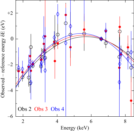
Figure 21: The differences between measured and reference energies of the brightest lines (see table 8 for details). The curves show the best-fit parabolic functions of the three observations.

Table 8: Emission lines used for energy-scale correction.

Ion Principal line Reference energy (eV) Observed shift $\delta E$ (eV) Ref. Name Transition Rest frame Observer frame Obs 2 Obs 3 Obs 4 Instrumental SiI K$\alpha_{1}$ 2p^-1 (²P_3/2) – 1s^-1 (²S_1/2) 1739.99 1739.99 $-$2.41 $-$2.49 $-$2.22 1 Astronomical SiXIV Ly$\alpha_{1}$ 1s (²S_1/2) – 2p (²P_3/2) 2006.08 1971.44 $-$2.96 $-$2.57 $-$2.32 2 SiXIV Ly$\beta_{1}$ 1s (²S_1/2) – 3p (²P_3/2) 2376.62 2335.58 $-$2.99 $-$2.17 $-$2.13 2 SXV He$\alpha$ w 1s² (¹S₀) – 1s.2p (¹P₁) 2460.63 2418.14 $-$3.44 $-$1.32 $-$1.74 3 SiXIV Ly$\gamma_{1}$ 1s (²S_1/2) – 4p (²P_3/2) 2506.37 2463.09 $-$0.63 $-$2.46 $-$3.37 2 SXVI Ly$\alpha_{1}$ 1s (²S_1/2) – 2p (²P_3/2) 2622.69 2577.40 $-$2.07 $-$1.95 $-$1.94 2 SXVI Ly$\beta_{1}$ 1s (²S_1/2) – 3p (²P_3/2) 3106.74 3053.10 $-$2.13 $-$1.62 $-$2.02 2 ArXVII He$\alpha$ w 1s² (¹S₀) – 1s.2p (¹P₁) 3139.77 3085.56 $-$1.38 $-$1.60 $-$1.85 4 SXVI Ly$\gamma_{1}$ 1s (²S_1/2) – 4p (²P_3/2) 3276.26 3219.69 $-$0.89 $-$0.38 $+$0.14 2 ArXVIII Ly$\alpha_{1}$ 1s (²S_1/2) – 2p (²P_3/2) 3322.98 3265.60 $-$0.97 $-$0.88 $-$1.51 2 SXVI Ly$\delta_{1}$ 1s (²S_1/2) – 5p (²P_3/2) 3354.73 3296.81 $-$1.46 $+$0.20 $-$2.44 2 CaXIX He$\alpha$ w 1s² (¹S₀) – 1s.2p (¹P₁) 3902.26 3834.88 $-$0.48 $-$0.24 $+$0.11 5 ArXVIII Ly$\beta_{1}$ 1s (²S_1/2) – 3p (²P_3/2) 3935.71 3867.75 $-$0.22 $-$1.71 — 2 CaXX Ly$\alpha_{1}$ 1s (²S_1/2) – 2p (²P_3/2) 4107.48 4036.56 $+$0.34 $-$0.34 $+$1.92 2 CaXIX He$\beta_{1}$ 1s² (¹S₀) – 1s.3p (¹P₁) 4582.81 4503.68 $+$1.22 $+$1.86 $-$0.31 5 CaXX Ly$\beta_{1}$ 1s (²S_1/2) – 3p (²P_3/2) 4864.08 4780.09 $+$0.33 $-$0.64 $+$0.99 2 CrXXIII He$\alpha$ w 1s² (¹S₀) – 1s.2p (¹P₁) 5682.05 5583.94 $+$0.42 $+$0.73 $+$3.53 6 FeXXV He$\alpha$ w 1s² (¹S₀) – 1s.2p (¹P₁) 6700.42 6584.73 0 6 FeXXVI Ly$\alpha_{1}$ 1s (²S_1/2) – 2p (²P_3/2) 6973.07 6852.67 $-$0.32 $+$0.60 $+$0.64 2 FeXXIV j₃ 2p (²P_3/2) – 1s.2p(³P).3p (²D_5/2) 7782.52 7648.14 $-$1.39 $-$2.23 $-$3.34 7 NiXXVII He$\alpha$ w 1s² (¹S₀) – 1s.2p (¹P₁) 7805.14 7670.37 $+$0.58 $+$0.94 $-$1.93 5 FeXXV He$\beta_{1}$ 1s² (¹S₀) – 1s.3p (¹P₁) 7881.12 7745.04 $-$0.94 $-$1.18 $-$1.21 5 FeXXV He$\gamma_{1}$ 1s² (¹S₀) – 1s.4p (¹P₁) 8295.39 8152.16 $-$1.09 $-$0.65 $-$1.54 5 FeXXV He$\delta_{1}$ 1s² (¹S₀) – 1s.5p (¹P₁) 8487.22 8340.67 $-$2.22 $-$4.77 $-$1.03 5

References: (1) Bearden (1967); (2) Erickson (1977); (3) Kaufman & Martin (1993); (4) Kelly (1987); (5) Sugar & Corliss (1985); (6) Shirai et al. (2000); (7) Calculations with the Flexible Atomic Code (Gu, 2008), A.J.J. Raassen, private comminication (2017).
A vacancy is denoted as a negative index of the electron configurations.
Poor fit. Ignored in derivation of the correction curve.
The energy shift at FeXXV He$\alpha$ is assumed to be zero as it is already adjusted by the removal of the spatial velocity gradient.
The 1s–3p analogous to the 1s–2p dielectronic satellite line, j: 2p (²P_3/2) – 1s.2p² (²D_5/2), labeled by Phillips (2008).

To obtain the energy-dependent residual energy-scale errors, we fit the strongest emission lines in the 1.9–9.5 keV band. For each line, we define an adjacent band with a width of 0.1–0.2 keV, and perform a local fit of the Hitomi SXS spectrum. Table 8 lists the principal lines for the individual bands. A collisional ionization equilibrium (CIE) model affected by redshift is used to fit the astronomical lines, whereas a redshifted double-Gaussian model is used for the instrumental Si K$\alpha$ lines. For the CIE model, the temperature is fixed to 4 keV, while the abundance, turbulent velocity, and redshift are left free. The redshift which is obtained from the fit is then compared with the known Perseus redshift ($z=$0.01756 or $cz=$5264 km s^-1: Ferruit et al., 1997) to obtain the best-fit energy shifts. The rest-frame reference energies implemented in the CIE model in SPEX version 3.03 are calculated values except for ArXVII He$\alpha$, each retrieved from the references shown in table 8. Some are not the most commonly used calculations or measurements for calibration, but the differences are usually much smaller than the statistical uncertainties in the present analysis and thus do not affect the correction results. Detailed comparisons of the reference energies are given in appendix B (table 9). For the instrumental Si lines, the relative normalization of the double Gaussians is fixed at the known value (Scofield, 1974), and the obtained redshift is directly converted to the energy shift. As shown in figure 21 and table 8, these shifts appear to be $-$(1–3) eV below 4 keV and above 7 keV, and $+$(0–2) eV in 4–7 keV. These differences cannot be justified by an astrophysical model — the $\sim$2 eV differences between the Si Ly$\alpha$ and Fe He$\alpha$ lines correspond to 300 km s^-1, while they are partially formed at similar temperatures. More importantly, at the high-energy side, there is a several eV difference in the Rydberg series of FeXXV, which is even harder to explain with a realistic astrophysical model. Furthermore, the energy-scale shifts at the instrumental Si K$\alpha$ lines are in good agreement with the parabolic trend of the astrophysical lines, providing further support for a non-astrophysical explanation.

The behavior of these deviations is consistent with calibration issues (Eckart et al., in prep.). As shown in figure 21, we perform an empirical fit using a parabolic function to the observed deviations ($\delta E$). The correction to the original energy $E$ (keV) is given as

$$c_{1}\cdot(E-E_{0})+c_{2}\cdot(E-E_{0})^{2}\mbox{~{}~{}eV}.$$ (1)

$E_{0}$ is the original energy at the Fe He$\alpha$ line, where the shift is fixed at zero as it has already been corrected by removal of the spacial velocity gradient. The best-fit values of the coefficients are ($c_{1}$, $c_{2}$) = (0.4062, 0.2281), (0.4882, 0.2360), and (0.6525, 0.2793) for Obs 2, 3, and 4, respectively. Similar corrections have been applied in other Hitomi Collaboration papers (Z, T, AGN, and RS papers).

We caution that this empirical correction is not to be used outside of the range of the fit or trusted at the extremes of that range. Because there is no mechanism for an offset in the energy scale, the error must eventually tend to 0 at the lowest energies.

A.2 Effective-area correction factor

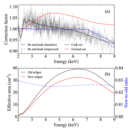
Figure 22: (a) A comparison of effective area correction factors: the original correction (blue) for each of the baseline and improved models respectively in solid and dashed curves, the on-ground calibration correction (red), and the Crab correction (black) derived by smoothing the SXS-to-canonical ratio (grey crosses: private communication with M. Tsujimoto, 2017). For the Crab analysis, the high-primary as well as mid-primary grade events are used. (b) Effective area with the old and the new aharfgen in black and red, respectively, as well as the ratio of the two calculations with the dashed blue curve.

To identify and remove any possible residual calibration errors on the effective area, which affects mostly the continuum spectrum, we incorporate two correction functions in the broad-band spectral analysis. One represents uncertainty in the thickness of the Be window of the gate valve, another the uncertainty in the effective area of the X-ray mirrors of the SXS. To estimate the size of these factors, the Hitomi SXS spectrum is rebinned into 100-eV bins to enhance the continuum features. We then fit it with the baseline model described later in section 3 incorporating a knak component which determines the correction function using piece-wise power-laws in energy-correction factor space, together with a neutral-Be absorption model.

By making several iterations between a fit with 100-eV wide bins and a fit with the optimal binning (see appendix A.3), the best-fit corrections and Be model are determined as shown with the solid curve in figure 22 (a). The fit prefers a negative absorption column of the Be model, which indicates that the actual thickness of the Be window might be slightly lower than the value (262 $\mu$m) used in the current calibration. The correction, however, approaches to unity with a more realistic spectral modeling of the ICM (an improved model; see section 10), as shown with the dashed curve in figure 22 (a). Therefore the thinner Be window preferred with the baseline model is most likely due to incomplete modeling of the ICM emission.

The best-fit effective-area correction function is consistent with unity at $\leq$7 keV, and decreases to 0.9 at $\sim$9 keV. This means that the current calibration might be underestimated by $\leq$10% at the high-energy end of the standard SXS bandpass. This correction above 7 keV is more significant with an improved model. We discuss the effective-area corrections in more detail in section C.4. Note that the sharp change at 7 keV is caused by the model grids; changing the grids has a negligible effect on the fitted parameters.

A.3 Binning of the data

For the binning of our X-ray data, we have followed the approach of Kaastra & Bleeker (2016) for optimal binning. The optimal bin size depends on the spectral resolution, number of resolution bins and local intensity of the spectrum and is different for each energy. It is achieved by issuing the obin command in SPEX. Since we started with spectrum with 0.5-eV resolution bin, our optimal bin size is a multiple of 0.5 eV. In practice, for most energies below 8.2 keV we use a bin size of 1.5 eV, and for higher energies 2 eV. The exceptions are near the SXV He$\alpha$ complex where we use 1 eV, and near the high-$n$ transition lines of FeXXV, including He$\gamma$, He$\delta$, and He$\varepsilon$ lines where we also use 1.5-eV data bins.

Appendix B Reference line energies for the energy-scale correction

Table 9 compares the reference energies of emission lines in SPEX used in the SXS energy-scale correction (appendix A.1) to the NIST Atomic Spectra Database version 5.3 (Kramida et al., 2016) and other available measurements and calculations.

In the case of hydrogenic ions, we use the calculations of Erickson (1977). This is in contrast to Hitomi Collaboration et al. (2016), where for H-like FeXXVI the calculations of Johnson & Soff (1985) were used. The up-to-date calculations of Yerokhin & Shabaev (2015) agree well with Johnson & Soff (1985). Although Johnson & Soff (1985) are the accepted standard for $n=$2 to 1 transitions in H-like ions (Ly$\alpha$) and have been well tested (Beiersdorfer, 2009), they do not include transitions from higher Rydberg states with $n\geq$3. The calculations are in good agreement between Erickson (1977) and Johnson & Soff (1985) within 0.02 eV for $Z\leq$20. For Ly$\alpha_{1}$ of FeXXVI, Erickson (1977) is 0.11 eV less. For consistency, we use the values from Erickson (1977).

For $n=$2 to 1 transitions in He-like ions (He$\alpha$) of Cr and Fe, Ca and Ni, and S, we respectively use the calculated values of Shirai et al. (2000), Sugar & Corliss (1985), and Kaufman & Martin (1993). For Ar He$\alpha$, we use the measurement of Kelly (1987). These values are in good agreements within 0.2 eV with the calculations of Artemyev et al. (2005) as well as Cheng et al. (1994). An exception is found in the Ni He$\alpha$ line, whose deviation is $+$0.47 eV. Recent update by Natarajan & Kadrekar (2013) gives a better agreement for Ni He$\alpha$ with the SPEX value. These calculations have also been compared to many measured values (Beiersdorfer & Brown, 2015), and good agreement is found. We also note the work of Drake (1988) which has been used often as a calibration standard.

For the 1s–3p transitions of FeXXV (He$\beta_{1}$) and FeXXIV (j₃ satellite in Phillips, 2008), we respectively use the calculation of Sugar & Corliss (1985) and a FAC calculation (private communication with A. J. J. Raassen, 2017). Smith et al. (1993) performed both calculations and measurements of these 1s–3p lines of Fe ions. The calculated values are in good agreements with those used in SPEX within 0.1 eV. On the other hand, the measured values have relatively large deviations ($-$0.45 and $-$0.9 eV, respectively) from the calculations, which may be due to the limited wavelength calibration of the crystal spectrometer, as noted in Smith et al. (1993).

For the other high-$n$ Rydberg series (CaXIX He$\beta$ and FeXXV He$\beta$–$\delta$), we use the calculated values from Sugar & Corliss (1985). The measurements of the high-$n$ lines of He-like FeXXV have been conducted by Indelicato et al. (1986) and Beiersdorfer et al. (1989), respectively. These agree well with the SPEX values within the measurement errors ($\pm$0.15 eV for He$\gamma_{1}$ and $\pm$0.22 eV for He$\delta_{1}$).

Appendix C Systematic factors due to instrumental effects

In this section we discuss the effects of several aspects of the instrumental calibrations on the derived parameters.

C.1 Velocity-gradient correction

The line broadening due to spatial bulk velocity of the ICM is removed by applying an energy-scale correction to each pixel (section 2). Without this correction, the C-statistic obtained with the baseline model increases by $\delta C_{\rm stat}=$62, and the LOS turbulent velocity dispersion becomes larger by 13 km s^-1 (“No vel. cor.” in table 1). The best-fit line center shifts towards shorter wavelength by 23 km s^-1.

C.2 Response matrices

We also test how much the fit changes by using a small RMF with only the Gaussian core component, as well as by using an extra-large RMF with the electron-loss continuum. As shown in table 1, a small RMF improves the baseline fit by $\delta C_{\rm stat}=$4, while an extra-large RMF (listed as “XL RMF”) gives instead a poorer fit with $\delta C_{\rm stat}=$12. The changes on the best-fit temperature and abundances by the RMF-type selection are 1–2%.

C.3 Non-X-ray background

The NXB rate depends on the orbital history of the satellite. Although this effect is already taken into account in sxsnxbgen, the systematic uncertainty could be large if the orbital history is biased. For the case of the Perseus observations (Obs 2–4), this systematic is expected to be small as the on-source time ($\approx$290 ks) is much longer than the satellite orbital period. Indeed, the estimated NXB rate is 3.0$\times$10^-2 counts s^-1 cm^-2 in 1.0–10 keV, consistent with the orbit-averaged value (Kilbourne et al., accepted.). This converts to 0.4% of the total count rate of the source events in 1.9–9.5 keV. Here, we consider an extreme case where we completely ignore the NXB contribution. As shown in table 1, the baseline run without the NXB component gives a larger C-statistic value ($\delta C_{\rm stat}=$9) than the original run, and the impact on the fitted parameters is minor, $\leq$1% on temperature and abundances.

C.4 Effective area

C.4.1 Point-source ARFs

The spatial extent of the target has an impact on the instrumental response. As shown in table 1 (labeled as “PS ARF”), the use of the point-source ARFs not only on the AGN component but also on the ICM component of the Perseus cluster gives a larger C-statistic value ($\delta C_{\rm stat}=$30) than the original baseline fit. The improper ARF would lead to a 1% bias on temperature and up to 5% biases on abundances.

C.4.2 No effective-area correction factor

The correction factor (appendix A.2) is included to remove potential calibration uncertainties on the effective area. As shown in table 1 (labeled as “No cor.”), ignoring the correction factor yields a poorer fit ($\delta C_{\rm stat}=$38). The temperature shifts by 0.08 keV from the original value, and several abundances are underestimated by 0.03 times solar. The emission measure changes by 1.3%, larger than the statistical error by a factor of 5. This indicates that the correction factor, despite being small, is still needed for the current calibration.

C.4.3 Correction factor based on on-ground calibration

The baseline effective area correction is done with the SPEX model knak. Alternatively, the correction can be achieved by setting auxtransfile=CALDB in the aharfgen run, which applies an additional empirical transmission on the original ARFs. With this correction, the discrepancy in the mirror effective area between on-ground calibration measurements and ray-tracing simulations are removed. We hence re-run the baseline fit by including the new correction factor while turning off the knak and Be-filter fine-tuning (appendix A.2). The original and new correction factors are respectively shown with the blue and red curves in figure 22 (a). A poorer fit ($\delta C_{\rm stat}=$191; “Ground cor.” in table 1) is obtained with the new correction, and the best-fit CIE emission measure changes by 4%. The temperature decreases by 0.12 keV and the abundances changes by $\leq$0.06 solar from the original values.

C.4.4 Correction using the Crab observation

The third method to evaluate and correct systematic uncertainty in effective area is to use standard candles. The Crab is one of the broadly used reference sources for effective area calibration. Using a 9.7-ks observation, Tsujimoto et al. (accepted.) found that the SXS spectrum of the Crab showed a systematic deviation from the canonical model. The deviation, defined as the SXS-to-canonical ratio, behaves differently depending on the energy bands, but in the 3–9 keV band it shows a monotonically decreasing trend on energy within $\pm$5%. This is reminiscent of our effective area correction with knak as shown in figure 22 (a). Therefore, we re-run the baseline fit with the Crab ratio as an effective-area correction instead of the original factor in appendix A.2.

As shown table 1 (“Crab cor.”), the Crab correction does improve the fit from the no-correction case (“No cor.”) by $\delta C_{\rm stat}=$25. This accounts for two-third of the improvement by using the original correction factor ($\delta C_{\rm stat}=$38). The slightly worse fit than the baseline model might be attributable to the different observation configurations between Perseus and Crab: different pixel contributions and event-grade selections due to different spatial extents of the sources and incoming photon rates.

C.4.5 ARF with the latest aharfgen

There has been released a newer version (006) of the Hitomi software including an updated ray-tracing ARF generator aharfgen, in which a bug in the coordinates calculation for an input image is corrected. A comparison of effective areas between the old and new tools, as well as the new-to-old area ratio are shown in figure 22 (b). The ratio curve has an almost constant, smooth structure over the fitting range without any line- or edge-like features. The notable difference is rather in the total effective area. The $\sim$20% lower area results in a comparable amount of increase in the ICM emission measure (“New arfgen” in table 1). Although the new ARF marginally improves the fit, any changes in the best-fit values of the other parameters are less than 0.1%, justifying the use of the old ARF in the baseline model for the current purpose.

C.5 Effects of the gain correction factor

The correction on energy scale is crucial for fitting the emission lines. Once it is removed, the fitting with the baseline model becomes worse by $\delta C_{\rm stat}=627$, and the Si, S, and Fe abundances are affected up to 15%. The temperature and line broadening are not affected by the energy-scale correction.

Appendix D Hitomi SXS spectral fits with different codes

Figures 23–25 show the full-band (1.9–9.5 keV) Hitomi SXS spectrum with the best-fit baseline model using SPEX version 3.03 and the relative differences of the best-fit models obtained with various other plasma models. See section 4 for details.

Appendix E List of emission lines

Tables E and 10 respectively compare the line energies $E$ of the strongest lines and satellite lines in the observed spectrum between different plasma codes. Einstein coefficient values $A$ and emissivities $\varepsilon$ are also compared. The emissivity thresholds are 10^-26 photons m³ s^-1 and 10^-25 photons m³ s^-1, respectively. See section 4 for details.

Table 9: Comparison of energies of emission lines used in the energy-scale correction.

Ion Principal line Rest-frame energy (eV) Deviation from SPEX (eV) $\sigma_{\rm SXS}$ Ref. Name Transition SPEX NIST v5 Others NIST v5 Others (eV) NIST v5 Others v3.03 Meas. Calc. Meas. Calc. Meas. Calc. Meas. Calc. M, C M, C SiXIV Ly$\alpha_{1}$ 1s (²S_1/2) – 2p (²P_3/2) 2006.08 — — — 2006.08 — — — 0.00 0.44 —, — —, (1) SiXIV Ly$\beta_{1}$ 1s (²S_1/2) – 3p (²P_3/2) 2376.62 — — — — — — — — 0.79 —, — —, — SXV He$\alpha$ w 1s² (¹S₀) – 1s.2p (¹P₁) 2460.63 2460.66 2460.62 2460.63 2460.629 0.03 $-$0.01 0.00 0.00 0.76 (2), (3) (4), (5) SiXIV Ly$\gamma_{1}$ 1s (²S_1/2) – 4p (²P_3/2) 2506.37 — — — — — — — — 1.15 —, — —, — SXVI Ly$\alpha_{1}$ 1s (²S_1/2) – 2p (²P_3/2) 2622.69 2622.6 2622.7 2622.704 2622.7 $-$0.1 0.0 0.01 0.0 0.22 (2), (6) (4), (1) SXVI Ly$\beta_{1}$ 1s (²S_1/2) – 3p (²P_3/2) 3106.74 — 3106.75 — — — 0.01 — — 0.47 —, (7) —, — ArXVII He$\alpha$ w 1s² (¹S₀) – 1s.2p (¹P₁) 3139.77 3139.585 3139.583 3139.58 3139.582 $-$0.19 $-$0.19 $-$0.19 $-$0.19 0.63 (8), (9) (4), (5) SXVI Ly$\gamma_{1}$ 1s (²S_1/2) – 4p (²P_3/2) 3276.26 — 3276.27 — — — 0.01 — — 1.12 —, (7) —, — ArXVIII Ly$\alpha_{1}$ 1s (²S_1/2) – 2p (²P_3/2) 3322.98 3322.990 3322.993 3322.993 3322.9932 0.01 0.01 0.01 0.01 0.44 (10), (1) (4), (11) SXVI Ly$\delta_{1}$ 1s (²S_1/2) – 5p (²P_3/2) 3354.73 — 3354.736 — — — 0.01 — — 2.42 —, (7) —, — CaXIX He$\alpha$ w 1s² (¹S₀) – 1s.2p (¹P₁) 3902.26 — — 3902.2 3902.378 — — 0.1 0.12 0.37 —, — (12), (5) ArXVIII Ly$\beta_{1}$ 1s (²S_1/2) – 3p (²P_3/2) 3935.71 — 3935.722 — — — 0.01 — — 1.74 —, (13) —, — CaXX Ly$\alpha_{1}$ 1s (²S_1/2) – 2p (²P_3/2) 4107.48 — — 4107.5 4107.5 — — 0.0 0.0 0.70 —, — (12), (1) CaXIX He$\beta_{1}$ 1s² (¹S₀) – 1s.3p (¹P₁) 4582.81 — — — — — — — — 3.44 —, — —, — CaXX Ly$\beta_{1}$ 1s (²S_1/2) – 3p (²P_3/2) 4864.08 — — — — — — — — 1.79 —, — —, — CrXXIII He$\alpha$ w 1s² (¹S₀) – 1s.2p (¹P₁) 5682.05 — 5681.9 5682.32 5682.068 — $-$0.2 0.27 0.02 1.61 —, (9) (14), (5) FeXXV He$\alpha$ w 1s² (¹S₀) – 1s.2p (¹P₁) 6700.42 — 6700.0 6700.55 6700.435 — $-$0.4 0.13 0.02 0.09 —, (9) (15), (5) FeXXVI Ly$\alpha_{1}$ 1s (²S_1/2) – 2p (²P_3/2) 6973.07 — 6973.179 6972.7348 6973.18 — 0.11 $-$0.34 0.11 0.44 —, (16) (17), (1) FeXXIV j₃ 2p (²P_3/2) – 1s.2p(³P).3p (²D_5/2) 7782.52 — — 7781.6 7782.6 — — $-$0.9 0.1 2.18 —, — (18), (18) NiXXVII He$\alpha$ w 1s² (¹S₀) – 1s.2p (¹P₁) 7805.14 — 7805.1 7804.6 7805.1 — 0.0 $-$0.5 0.0 1.31 —, (9) (19), (20) FeXXV He$\beta_{1}$ 1s² (¹S₀) – 1s.3p (¹P₁) 7881.12 — 7881.17 7880.67 7881.0 — 0.05 $-$0.45 $-$0.1 0.42 —, (16) (18), (18) FeXXV He$\gamma_{1}$ 1s² (¹S₀) – 1s.4p (¹P₁) 8295.39 — 8295.48 8295.64 — — 0.09 0.25 — 0.81 —, (16) (21), — FeXXV He$\delta_{1}$ 1s² (¹S₀) – 1s.5p (¹P₁) 8487.22 — 8487.3 8487.36 — — 0.1 0.14 — 1.67 —, (16) (14), —

Line energies in SPEX v3.03 and measured and calculated values in the NIST Atomic Spectra Database v5.3 (NIST v5: Kramida et al., 2016) and those in other calibration standards.
Statistical errors in line energy shift measurements with the Hitomi SXS. Those of the three observations (Obs 2, 3, and 4) are averaged by taking root mean squares.
References for the measured (M) and calculated (C) values in NIST v5 and those in other results: (1) Johnson & Soff (1985); (2) Schleinkofer et al. (1982); (3) Aglitsky et al. (1988); (4) Kubiček et al. (2014); (5) Artemyev et al. (2005); (6) Aglitskii et al. (1974); (7) Kaufman & Martin (1993); (8) Bruhns et al. (2007); (9) Kramida et al. (2016); (10) Beyer et al. (1985); (11) Yerokhin & Shabaev (2015); (12) Rice et al. (2014); (13) Erickson (1977); (14) Beiersdorfer et al. (1989); (15) Rudolph et al. (2013); (16) Shirai et al. (2000); (17) Chantler et al. (2007); (18) Smith et al. (1993); (19) Bombarda et al. (1988); (20) Natarajan & Kadrekar (2013); (21) Indelicato et al. (1986).
For the references for the line energies in SPEX version 3.03, see table 8.
The 1s–3p analogous to the 1s–2p DR satellite line, j: 2p (²P_3/2) – 1s.2p² (²D_5/2), labeled by Phillips (2008).

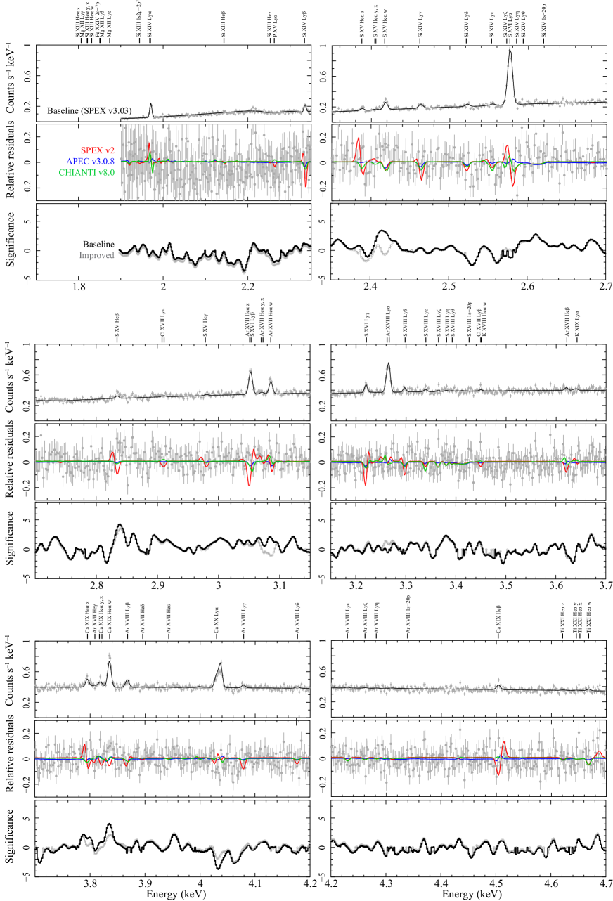
Figure 23: The SXS spectrum of the Perseus cluster in 1.9–4.7 keV fitted with different models. Panels in each subfigure show (upper) fit to the data with the baseline model, (middle) relative difference between the baseline model and the best-fit models with APEC v3.0.8 in blue, SPEX v2 in red, and CHIANTI v8.0 in green, and (lower) significances in $\sigma$ of an additional line model at each energy on top of the baseline model in black and improved model in grey.

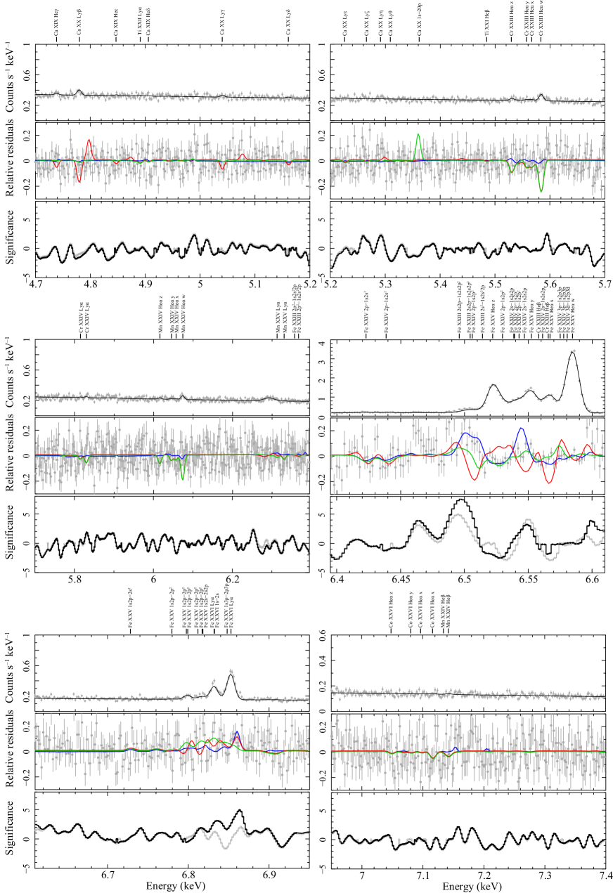
Figure 24: The same as figure 23, but in 4.7–7.4 keV.

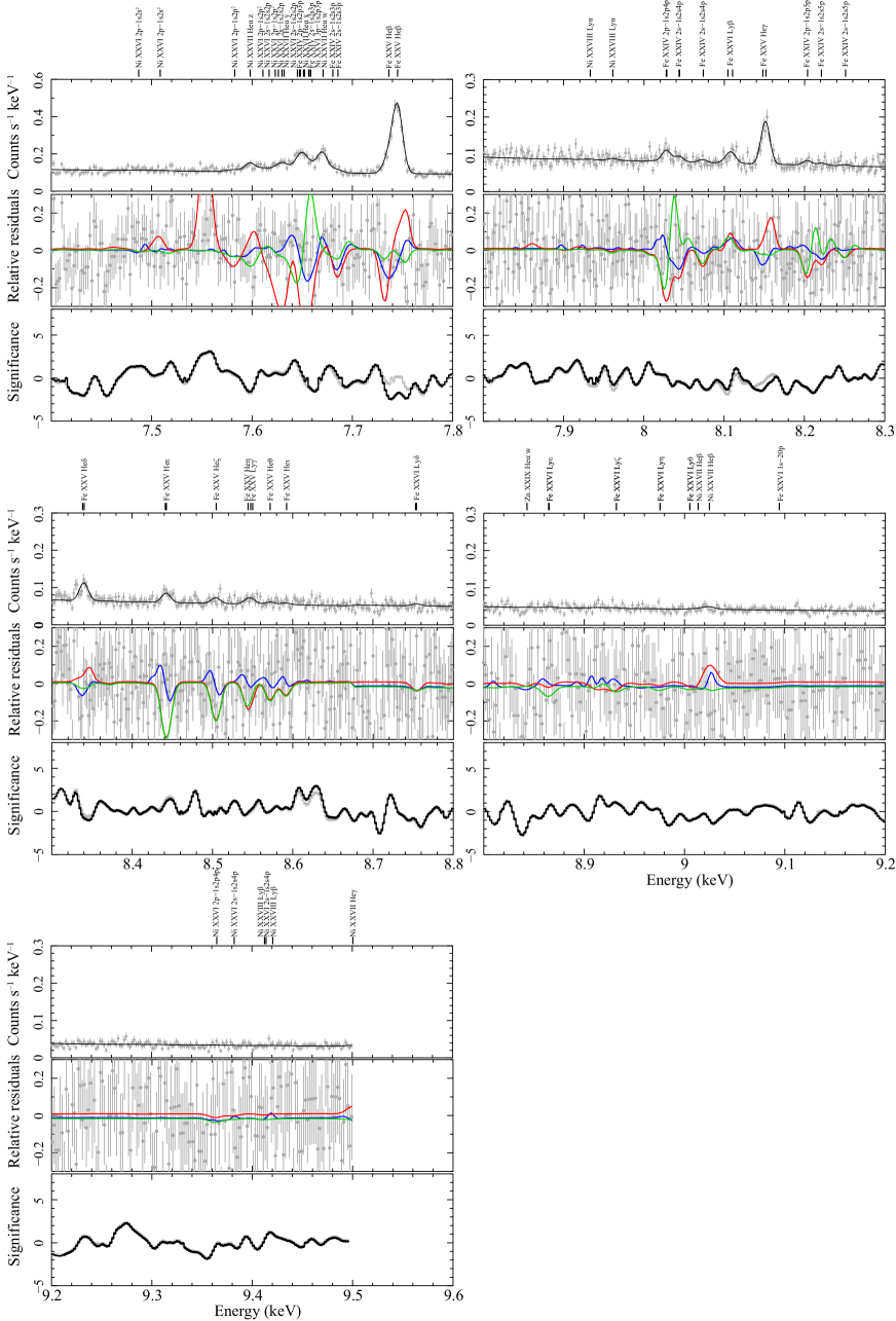
Figure 25: The same as figure 23, but in 7.4–9.5 keV.

@lccccccccccccc Comparisons of energies, transition probabilities, and emissivities of Lyman- and Helium-series lines for flux calculation. Name $E$ (keV) $f_{E}$ $\log_{10}A$ (s^-1) $f_{A}$ $\varepsilon$ (10^-23 m³ s^-1) $f_{\varepsilon}$
S3 A S2 C (%) S3 A C (%) S3 A C (%)
Name $E$ (keV) $f_{E}$ $\log_{10}A$ (s^-1) $f_{A}$ $\varepsilon$ (10^-23 m³ s^-1) $f_{\varepsilon}$
S3 A S2 C (%) S3 A C (%) S3 A C (%)
Energies $E$, Einstein $A$ values, and emissivities $\varepsilon$ in SPEX v3.03 (S3), AtomDB/APEC v3.0.8 (A), SPEX v2 (S2), and CHIANTI v8.0 (C).
Coefficient of variation (standard deviation divided by the mean) on energies $E$, $A$ values, and emissivities $\varepsilon$.
SiXIV Ly$\alpha_{2}$ 2.00432 2.00432 2.00395 2.00434 0.008 13.3827 13.3811 13.3831 0.2 0.905 0.856 1.140 12.8
SiXIV Ly$\alpha_{1}$ 2.00608 2.00608 2.00589 2.00609 0.004 13.3836 13.3822 13.3845 0.2 1.808 1.706 2.270 12.7
SiXIV Ly$\beta_{2}$ 2.37610 2.37610 2.37518 2.37609 0.017 12.8096 12.8061 12.8098 0.4 0.147 0.132 0.150 5.5
SiXIV Ly$\beta_{1}$ 2.37662 2.37662 (2.37518) 2.37663 0.026 12.8099 12.8094 12.8106 0.1 0.294 0.264 0.300 5.5
SiXIV Ly$\gamma_{2}$ 2.50615 2.50615 2.50473 2.50615 0.025 12.4201 12.4156 12.4201 0.5 0.054 0.044 0.048 8.4
SiXIV Ly$\gamma_{1}$ 2.50637 2.50637 (2.50473) 2.50635 0.028 12.4200 12.4198 12.4209 0.1 0.108 0.089 0.095 8.1
SiXIV Ly$\delta_{2}$ 2.56632 2.56632 2.56696 2.56632 0.011 12.1225 12.1176 12.1229 0.6 0.026 0.020 0.021 11.8
SiXIV Ly$\delta_{1}$ 2.56643 2.56643 (2.56696) 2.56643 0.009 12.1225 12.1222 12.1235 0.1 0.052 0.041 0.043 10.6
SiXIV Ly$\varepsilon_{2}$ 2.59899 2.59899 2.59925 — 0.005 11.8815 11.8764 — 0.6 0.013 0.011 — 8.3
SiXIV Ly$\varepsilon_{1}$ 2.59905 2.59906 (2.59925) — 0.004 11.8815 11.8812 — 0.0 0.026 0.022 — 8.3
SiXIV Ly$\zeta_{2}$ 2.61868 2.61869 — — 0.000 11.6759 11.6732 — 0.3 0.008 0.007 — 6.7
SiXIV Ly$\zeta_{1}$ 2.61872 2.61873 — — 0.000 11.6760 11.6781 — 0.2 0.016 0.013 — 10.3
PXV Ly$\alpha_{2}$ 2.30165 2.30165 — 2.30163 0.000 13.5030 13.4991 13.5032 0.4 0.009 0.009 0.011 9.8
PXV Ly$\alpha_{1}$ 2.30396 2.30396 — 2.30394 0.000 13.5039 13.5005 13.5047 0.4 0.019 0.018 0.022 8.6
SXVI Ly$\alpha_{2}$ 2.61969 2.61969 2.61957 2.61968 0.002 13.6153 13.6110 13.6157 0.5 0.580 0.524 0.684 11.1
SXVI Ly$\alpha_{1}$ 2.62269 2.62269 2.62179 2.62267 0.015 13.6165 13.6125 13.6173 0.5 1.160 1.044 1.370 11.3
SXVI Ly$\beta_{2}$ 3.10585 3.10585 3.10737 3.10582 0.021 13.0422 13.3365 13.0426 34.5 0.091 0.079 0.089 6.1
SXVI Ly$\beta_{1}$ 3.10674 3.10674 (3.10737) 3.10675 0.009 13.0426 13.3387 13.0434 34.7 0.183 0.158 0.179 6.3
SXVI Ly$\gamma_{2}$ 3.27589 3.27589 3.28001 3.27584 0.055 12.6527 12.6376 12.6528 1.6 0.032 0.026 0.028 8.7
SXVI Ly$\gamma_{1}$ 3.27626 3.27626 (3.28001) 3.27628 0.049 12.6527 12.6377 12.6536 1.7 0.065 0.053 0.057 8.6
SXVI Ly$\delta_{2}$ 3.35454 3.35454 3.35093 3.35455 0.047 12.3553 12.6419 12.3555 33.6 0.016 0.012 0.013 12.4
SXVI Ly$\delta_{1}$ 3.35473 3.35473 (3.35093) 3.35473 0.049 12.3553 12.3328 12.3562 2.5 0.032 0.024 0.025 13.2
SXVI Ly$\varepsilon_{2}$ 3.39724 3.39731 3.39683 — 0.006 12.1143 12.0824 — 3.7 0.008 0.006 — 14.3
SXVI Ly$\varepsilon_{1}$ 3.39724 3.39742 (3.39683) — 0.007 12.1143 12.0824 — 3.7 0.016 0.013 — 10.3
SXVI Ly$\zeta_{2}$ 3.42298 3.42305 — — 0.001 11.9076 11.8666 — 4.7 0.005 0.004 — 11.1
SXVI Ly$\zeta_{1}$ 3.42298 3.42312 — — 0.002 11.9077 11.8666 — 4.7 0.010 0.008 — 11.1
ClXVII Ly$\alpha_{2}$ 2.95851 2.95853 — 2.95849 0.001 13.7210 13.7159 13.7214 0.6 0.008 0.014 0.009 25.4
ClXVII Ly$\alpha_{1}$ 2.96234 2.96235 — 2.96230 0.001 13.7223 13.7177 13.7231 0.6 0.016 0.027 0.018 23.5
ClXVII Ly$\beta_{2}$ 3.50770 3.50771 — 3.50773 0.000 13.1480 13.4411 13.1483 34.4 0.001 0.002 0.001 35.4
ClXVII Ly$\beta_{1}$ 3.50884 3.50884 — 3.50882 0.000 13.1483 13.4437 13.1489 34.6 0.003 0.004 0.002 27.2
ArXVIII Ly$\alpha_{2}$ 3.31816 3.31816 3.31775 3.31775 0.006 13.8207 13.8149 13.8191 0.6 0.160 0.148 0.150 3.4
ArXVIII Ly$\alpha_{1}$ 3.32298 3.32298 3.32308 3.32308 0.002 13.8221 13.8168 13.8165 0.6 0.320 0.294 0.270 6.9
ArXVIII Ly$\beta_{2}$ 3.93428 3.93428 3.93601 3.93426 0.019 13.2475 13.5397 13.2435 34.5 0.024 0.022 0.018 11.7
ArXVIII Ly$\beta_{1}$ 3.93571 3.93571 (3.93601) 3.93576 0.003 13.2480 13.5427 13.2438 34.8 0.049 0.044 0.036 12.5
ArXVIII Ly$\gamma_{2}$ 4.14973 4.14973 — 4.14968 0.001 12.8581 12.8387 12.8532 1.9 0.008 0.007 0.006 11.7
ArXVIII Ly$\gamma_{1}$ 4.15033 4.15033 — 4.15038 0.001 12.8581 12.8388 12.8550 1.9 0.017 0.015 0.011 17.4
ArXVIII Ly$\delta_{2}$ 4.24936 4.24936 — 4.24938 0.000 12.5606 12.5319 12.5547 2.8 0.004 0.003 0.003 14.1
ArXVIII Ly$\delta_{1}$ 4.24967 4.24967 — 4.24967 0.000 12.5607 12.5319 12.5565 2.9 0.008 0.007 0.005 18.7
KXIX Ly$\alpha_{2}$ 3.69868 3.69869 — 3.69870 0.000 13.9150 13.9084 13.9152 0.7 0.006 0.006 0.007 7.4
KXIX Ly$\alpha_{1}$ 3.70466 3.70468 — 3.70467 0.000 13.9165 13.9105 13.9173 0.7 0.013 0.012 0.014 6.3
CaXX Ly$\alpha_{2}$ 4.10012 4.10012 4.10069 4.10014 0.006 14.0043 13.9971 14.0048 0.8 0.095 0.089 0.103 6.0
CaXX Ly$\alpha_{1}$ 4.10748 4.10748 4.10748 4.10748 0.000 14.0060 13.9994 14.0069 0.8 0.190 0.177 0.206 6.2
CaXX Ly$\beta_{2}$ 4.86190 4.86190 4.88127 4.86193 0.172 13.4315 13.7214 13.4317 34.0 0.014 0.013 0.013 3.5
CaXX Ly$\beta_{1}$ 4.86408 4.86408 (4.88127) 4.86403 0.153 13.4320 13.7250 13.4328 34.3 0.028 0.026 0.027 3.0
CaXX Ly$\gamma_{2}$ 5.12822 5.12822 5.16601 5.12819 0.319 13.0418 13.0179 13.0422 2.6 0.005 0.004 0.004 10.9
CaXX Ly$\gamma_{1}$ 5.12914 5.12914 (5.16601) 5.12925 0.310 13.0422 13.0179 13.0430 2.7 0.009 0.008 0.008 5.7
CaXX Ly$\delta_{2}$ 5.25136 5.25136 5.39062 5.25134 1.141 12.7445 12.7087 12.7447 3.8 0.002 0.002 0.002 0.0
CaXX Ly$\delta_{1}$ 5.25183 5.25183 (5.39062) 5.25179 1.137 12.7446 12.7088 12.7455 3.9 0.005 0.004 0.004 10.9
TiXXII Ly$\alpha_{2}$ 4.96605 4.96609 — — 0.000 14.1708 14.1617 — 1.1 0.002 0.002 — 0.0
TiXXII Ly$\alpha_{1}$ 4.97685 4.97689 — — 0.000 14.1729 14.1647 — 0.9 0.005 0.004 — 11.1
CrXXIV Ly$\alpha_{2}$ 5.91644 5.91650 — — 0.001 14.3230 14.3120 — 1.3 0.005 0.005 — 0.0
CrXXIV Ly$\alpha_{1}$ 5.93178 5.93185 — — 0.001 14.3253 14.3153 — 1.1 0.011 0.009 — 10.0
MnXXV Ly$\alpha_{2}$ 6.42349 6.42356 — — 0.001 14.3945 14.3824 — 1.4 0.002 0.001 — 33.3
MnXXV Ly$\alpha_{1}$ 6.44159 6.44166 — — 0.001 14.3971 14.3860 — 1.3 0.004 0.003 — 14.3
FeXXVI Ly$\alpha_{2}$ 6.95186 6.95186 6.95186 6.95212 0.002 14.4630 14.4499 14.4634 1.4 0.100 0.099 0.114 6.6
FeXXVI Ly$\alpha_{1}$ 6.97307 6.97307 6.97307 6.97324 0.001 14.4658 14.4538 14.4667 1.4 0.209 0.194 0.212 3.8
FeXXVI Ly$\beta_{2}$ 8.24629 8.24629 8.25051 8.24637 0.022 13.8904 14.1720 13.8906 33.0 0.012 0.013 0.015 9.4
FeXXVI Ly$\beta_{1}$ 8.25258 8.25258 (8.25051) 8.25241 0.011 13.8911 14.1781 13.8919 33.6 0.023 0.025 0.027 6.5
FeXXVI Ly$\gamma_{2}$ 8.69847 8.69847 8.70004 8.69881 0.007 13.5009 13.4589 13.5011 4.5 0.004 0.004 0.004 0.0
FeXXVI Ly$\gamma_{1}$ 8.70112 8.70113 (8.70004) 8.70126 0.006 13.5011 13.4592 13.5020 4.5 0.008 0.008 0.008 0.0
FeXXVI Ly$\delta_{2}$ 8.90740 8.90740 8.90831 8.90755 0.004 13.2036 13.4651 13.2036 30.5 0.002 0.002 0.002 0.0
FeXXVI Ly$\delta_{1}$ 8.90876 8.90876 (8.90831) 8.90883 0.002 13.2036 13.1411 13.2044 6.7 0.005 0.004 0.004 10.9
FeXXVI Ly$\varepsilon_{2}$ 9.02074 9.02104 9.02076 — 0.002 12.9624 12.8740 — 10.1 0.001 0.001 — 0.0
FeXXVI Ly$\varepsilon_{1}$ 9.02076 9.02182 (9.02076) — 0.006 12.9624 12.8739 — 10.2 0.002 0.002 — 0.0
FeXXVI Ly$\zeta_{2}$ 9.08901 9.08931 — — 0.002 12.7490 12.6348 — 13.1 0.001 0.001 — 0.0
FeXXVI Ly$\zeta_{1}$ 9.08902 9.08980 — — 0.004 12.7490 12.6347 — 13.1 0.001 0.001 — 0.0
NiXXVIII Ly$\alpha_{2}$ 8.07296 8.07420 8.07296 8.07294 0.007 14.5930 14.5775 14.5933 1.7 0.002 0.002 0.002 0.0
NiXXVIII Ly$\alpha_{1}$ 8.10160 8.10160 8.10160 8.10195 0.002 14.5962 14.5821 14.5970 1.6 0.004 0.003 0.004 12.9
NiXXVIII Ly$\beta_{2}$ 9.57743 9.57743 9.58359 9.57777 0.027 14.0204 14.2986 14.0208 32.6 0.0002 0.0002 0.0002 0.0
NiXXVIII Ly$\beta_{1}$ 9.58592 9.58592 (9.58359) 9.58591 0.011 14.0212 13.9916 14.0220 3.2 0.0005 0.0004 0.0005 10.1

SXV He$\alpha$ z 2.43035 2.43035 2.42631 2.43035 0.072 6.1553 6.1206 6.1553 3.7 0.084 0.083 0.061 14.0
SXV He$\alpha$ y 2.44714 2.44714 2.44704 2.44714 0.002 11.7686 11.6702 11.6826 10.4 0.026 0.026 0.021 9.7
SXV He$\alpha$ x 2.44876 2.44876 — 2.44878 0.000 8.0755 8.0682 8.0755 0.8 0.012 0.012 0.010 8.3
SXV He$\alpha$ w 2.46063 2.46063 2.46054 2.46064 0.002 13.8180 13.8261 13.8242 0.8 0.294 0.255 0.269 5.9
SXV He$\beta_{2}$ 2.88022 2.88022 2.87667 2.88021 0.053 11.2098 11.1644 11.1898 4.3 0.0010 0.0010 0.0006 21.8
SXV He$\beta_{1}$ 2.88392 2.88403 (2.87667) 2.88396 0.110 13.2591 13.2672 13.2651 0.8 0.047 0.044 0.043 3.8
SXV He$\gamma_{2}$ 3.03099 3.03099 3.02401 3.03095 0.100 10.8455 10.7853 10.8307 5.8 0.0002 0.0002 0.0002 0.0
SXV He$\gamma_{1}$ 3.03251 3.03266 (3.02401) 3.03251 0.122 12.8721 12.8785 12.8779 0.7 0.017 0.016 0.015 5.1
ArXVII He$\alpha$ z 3.10435 3.10414 3.107374 3.10426 0.044 6.6812 6.6484 6.6473 3.7 0.051 0.050 0.041 9.5
ArXVII He$\alpha$ y 3.12374 3.12353 3.12303 3.12374 0.009 12.2601 12.1644 12.2235 9.0 0.019 0.018 0.016 7.1
ArXVII He$\alpha$ x 3.12647 3.12628 — 3.12673 0.006 8.4997 8.4940 8.5068 1.2 0.013 0.013 0.011 7.6
ArXVII He$\alpha$ w 3.13977 3.13958 3.13884 3.13940 0.011 14.0302 14.0374 14.0527 2.2 0.178 0.161 0.166 4.2
ArXVII He$\beta_{2}$ 3.67961 3.67943 3.70102 3.67938 0.253 11.6984 11.6551 11.7005 4.7 0.0010 0.0010 0.0007 15.7
ArXVII He$\beta_{1}$ 3.68404 3.68452 (3.70102) 3.68233 0.205 13.4642 13.4742 13.5406 8.0 0.027 0.026 0.025 3.1
ArXVII He$\gamma_{2}$ 3.87301 3.87301 — 3.87305 0.000 11.3328 11.2718 11.3422 7.0 0.0003 0.0002 0.0002 20.2
ArXVII He$\gamma_{1}$ 3.87504 3.87451 — 3.87487 0.006 13.0730 13.0792 13.2443 19.3 0.010 0.009 0.008 9.1
KXVIII He$\alpha$ z 3.47218 3.47229 — 3.47217 0.002 6.9229 6.8899 6.9188 3.3 0.003 0.004 0.002 27.2
KXVIII He$\alpha$ y 3.49297 3.49302 — 3.49301 0.001 12.4800 12.3874 12.4806 9.7 0.0010 0.0010 0.0008 10.1
KXVIII He$\alpha$ x 3.49646 3.49654 — 3.49645 0.001 8.6940 8.6890 8.6923 0.5 0.0010 0.0010 0.0006 21.8
KXVIII He$\alpha$ w 3.51036 3.51051 — 3.51031 0.002 14.1258 14.1335 14.1294 0.7 0.011 0.010 0.010 4.6
CaXIX He$\alpha$ z 3.86114 3.86120 3.85871 3.86111 0.027 7.1523 7.1173 7.1523 3.7 0.066 0.069 0.058 7.2
CaXIX He$\alpha$ y 3.88332 3.88331 3.88118 3.88336 0.024 12.6848 12.5944 12.6022 9.7 0.028 0.038 0.037 13.1
CaXIX He$\alpha$ x 3.88770 3.88775 3.88544 3.88775 0.026 8.8779 8.8736 8.8779 0.5 0.024 0.027 0.025 4.9
CaXIX He$\alpha$ w 3.90226 3.90237 3.90219 3.90243 0.002 14.2156 14.2227 14.2214 0.7 0.226 0.236 0.241 2.7
CaXIX He$\beta_{2}$ 4.57753 4.57753 4.59201 4.57760 0.137 12.1565 12.0792 12.1014 7.6 0.002 0.002 0.002 0.0
CaXIX He$\beta_{1}$ 4.58281 4.58352 (4.59201) 4.58284 0.085 13.6437 13.6551 13.6542 1.2 0.033 0.038 0.038 6.5
CaXIX He$\gamma_{2}$ 4.81941 4.81941 4.76863 4.81941 0.457 11.7916 11.6893 11.7362 9.7 0.0010 0.0010 0.0005 28.3
CaXIX He$\gamma_{1}$ 4.82158 4.82241 (4.76863) 4.82166 0.480 13.2529 13.2577 13.2608 0.8 0.011 0.012 0.012 4.0
CaXIX He$\delta_{2}$ 4.93107 4.93107 4.95937 4.93116 0.248 11.4986 11.3522 11.4456 13.6 0.0003 0.0002 0.0002 20.2
CaXIX He$\delta_{1}$ 4.93217 4.93175 (4.95937) 4.93214 0.240 12.9553 12.9294 12.9549 2.8 0.005 0.005 0.005 0.0
TiXXI He$\alpha$ z 4.70196 4.70196 — — 0.000 7.5755 7.5428 — 3.8 0.003 0.003 — 0.0
TiXXI He$\alpha$ y 4.72693 4.72693 — — 0.000 13.0326 12.9657 — 7.7 0.002 0.002 — 0.0
TiXXI He$\alpha$ x 4.73379 4.73379 — — 0.000 9.2193 9.2159 — 0.4 0.002 0.001 — 33.3
TiXXI He$\alpha$ w 4.74963 4.74963 — — 0.000 14.3798 14.3874 — 0.9 0.012 0.010 — 9.1
CrXXIII He$\alpha$ z 5.62691 5.62691 — — 0.000 7.9622 7.9304 — 3.7 0.017 0.019 — 5.6
CrXXIII He$\alpha$ y 5.65484 5.65484 — — 0.000 13.3458 13.2900 — 6.4 0.010 0.009 — 5.3
CrXXIII He$\alpha$ x 5.66506 5.66506 — — 0.000 9.5306 9.5278 — 0.3 0.009 0.009 — 0.0
CrXXIII He$\alpha$ w 5.68205 5.68205 — — 0.000 14.5271 14.5353 — 0.9 0.056 0.049 — 6.7
CrXXIII He$\beta_{2}$ 6.67313 6.67313 — — 0.000 12.8927 12.7559 — 15.6 0.001 0.001 — 0.0
CrXXIII He$\beta_{1}$ 6.68077 6.68077 — — 0.000 13.9577 13.9600 — 0.3 0.008 0.007 — 6.7
MnXXIV He$\alpha$ z 6.12105 6.12113 — — 0.001 8.1436 8.1106 — 3.8 0.011 0.008 — 15.8
MnXXIV He$\alpha$ y 6.15071 6.15057 — — 0.001 13.4933 13.4346 — 6.8 0.007 0.004 — 27.3
MnXXIV He$\alpha$ x 6.16284 6.16290 — — 0.000 9.6765 9.6739 — 0.3 0.006 0.004 — 20.0
MnXXIV He$\alpha$ w 6.18019 6.18044 — — 0.002 14.5949 14.6042 — 1.1 0.034 0.022 — 21.4
MnXXIV He$\beta_{2}$ 7.25981 7.25983 — — 0.000 13.0406 12.8965 — 16.4 0.001 0.000 — 17.6
MnXXIV He$\beta_{1}$ 7.26822 7.26826 — — 0.000 14.0278 14.0253 — 0.3 0.004 0.003 — 14.3
FeXXV He$\alpha$ z 6.63660 6.63658 6.63652 6.63656 0.000 8.3181 8.2856 8.3181 3.5 0.826 0.737 0.758 4.9
FeXXV He$\alpha$ y 6.66757 6.66755 6.66777 6.66761 0.001 13.6294 13.5705 13.6385 6.8 0.544 0.474 0.516 5.6
FeXXV He$\alpha$ x 6.68233 6.68230 6.68220 6.68234 0.001 9.8162 9.8142 9.8116 0.4 0.491 0.442 0.472 4.3
FeXXV He$\alpha$ w 6.70042 6.70040 6.70011 6.70076 0.003 14.6594 14.6693 14.6637 0.9 2.568 2.197 2.440 6.4
FeXXV He$\beta_{2}$ 7.87185 7.87202 7.88112 7.87201 0.050 13.1830 13.0253 13.0515 16.6 0.062 0.047 0.051 11.9
FeXXV He$\beta_{1}$ 7.88112 7.88152 (7.88112) 7.88102 0.002 14.0934 14.0899 14.0885 0.5 0.328 0.293 0.316 4.6
FeXXV He$\gamma_{2}$ 8.29154 8.29160 8.29539 8.29159 0.020 12.7757 12.6191 12.6732 15.3 0.019 0.014 0.015 13.5
FeXXV He$\gamma_{1}$ 8.29539 8.29548 (8.29539) 8.29548 0.001 13.7029 13.6776 13.6845 2.5 0.102 0.092 0.099 4.3
FeXXV He$\delta_{2}$ 8.48526 8.48510 8.48722 8.48509 0.011 12.4947 12.2430 12.3698 23.4 0.008 0.006 0.006 14.1
FeXXV He$\delta_{1}$ 8.48722 8.48742 (8.48722) 8.48742 0.001 13.4052 13.3139 13.3662 8.5 0.045 0.041 0.043 3.8
FeXXV He$\varepsilon_{2}$ 8.59032 8.58733 — — 0.017 12.2492 12.1199 — 14.8 0.004 0.004 — 0.0
FeXXV He$\varepsilon_{1}$ 8.59145 8.58848 — — 0.017 13.2188 13.1086 — 12.6 0.024 0.024 — 0.0
FeXXV He$\zeta_{2}$ 8.65361 8.65058 — — 0.018 12.0558 11.8927 — 18.6 0.003 0.002 — 20.0
FeXXV He$\zeta_{1}$ 8.65433 8.65130 — — 0.018 13.0166 12.8733 — 16.4 0.015 0.014 — 3.4
FeXXV He$\eta_{2}$ 8.69451 8.69158 — — 0.017 11.8935 11.6734 — 24.8 0.002 0.001 — 33.3
FeXXV He$\eta_{1}$ 8.69499 8.69206 — — 0.017 12.8416 12.6465 — 22.1 0.010 0.009 — 5.3
FeXXV He$\theta_{2}$ 8.72260 8.71967 — — 0.017 11.7612 11.4252 — 36.9 0.001 0.001 — 0.0
FeXXV He$\theta_{1}$ 8.72294 8.72001 — — 0.017 12.6870 12.3902 — 32.9 0.006 0.006 — 0.0
FeXXV He$\iota_{2}$ 8.74267 8.73975 — — 0.017 11.6770 10.9255 — 69.9 0.001 0.001 — 0.0
FeXXV He$\iota_{1}$ 8.74292 8.73999 — — 0.017 12.5488 11.8781 — 64.8 0.004 0.004 — 0.0
CoXXVI He$\alpha$ z 7.17332 7.18465 — — 0.079 8.4864 8.4533 — 3.8 0.002 — — —
CoXXVI He$\alpha$ y 7.20619 7.21658 — — 0.072 13.7560 13.6972 — 6.8 0.001 — — —
CoXXVI He$\alpha$ x 7.22341 7.23461 — — 0.077 9.9498 9.9490 — 0.1 0.001 — — —
CoXXVI He$\alpha$ w 7.24173 7.25408 — — 0.085 14.7208 14.7308 — 1.1 0.006 — — —
NiXXVII He$\alpha$ z 7.73153 7.73161 7.73162 7.73162 0.000 8.6484 8.6138 8.6484 3.7 0.031 0.032 0.029 4.1
NiXXVII He$\alpha$ y 7.76605 7.76567 7.77867 7.76600 0.071 13.8745 13.8149 13.8171 6.5 0.022 0.021 0.022 2.2
NiXXVII He$\alpha$ x 7.78637 7.78642 — 7.78649 0.001 10.0792 10.0788 10.0792 0.0 0.020 0.019 0.020 2.4
NiXXVII He$\alpha$ w 7.80514 7.80556 7.80511 7.80511 0.002 14.7795 14.7903 14.7893 1.1 0.091 0.081 0.088 4.8

NiXXVII He$\beta_{2}$ 9.17227 9.17043 9.18358 9.17246 0.057 13.3863 13.2625 13.2869 12.7 0.003 0.002 0.002 20.2
NiXXVII He$\beta_{1}$ 9.18359 9.18402 (9.18358) 9.18333 0.003 14.2135 14.2068 14.2057 0.8 0.011 0.010 0.011 4.4
NiXXVII He$\gamma_{2}$ 9.66241 9.66362 9.66712 9.66211 0.021 12.9997 12.8451 12.9032 14.9 0.0008 0.0006 0.0006 14.1
NiXXVII He$\gamma_{1}$ 9.66711 9.66362 (9.66712) 9.66738 0.016 13.8048 13.7903 13.7979 1.4 0.003 0.003 0.003 0.0

Table 10: The same as table E, but for satellite lines.

Line $E$ (keV) $f_{E}$ $\log_{10}A$ (s^-1) $f_{A}$ $\varepsilon$ (10^-23 m³ s^-1) $f_{\varepsilon}$ Transition Key S3 A S2 C (%) S3 A C (%) S3 A C (%) L-shell lines He-like FeXXV 1s.2s ³S₁ – 1s.5p ³P₂ 1.84960 1.84966 — 1.84971 0.002 12.2967 12.1875 12.2487 10.2 0.014 0.011 0.011 11.8 Li-like FeXXIV 2p ²P_3/2 – 7s ²S_1/2 1.81905 1.81893 — 1.81990 0.024 11.1216 11.1216 10.8681 24.4 0.012 0.009 — 14.3 2p ²P_3/2 – 7d ²D_5/2 1.82117 1.82679 — 1.82107 0.147 12.0434 12.0430 12.0043 4.2 0.028 0.030 0.006 51.0 2s ²S_1/2 – 6p ²P_1/2 1.82640 1.82634 1.82625 1.82641 0.003 11.9879 11.9993 11.9330 6.5 0.039 0.033 0.006 55.2 2s ²S_1/2 – 6p ²P_3/2 1.82698 1.82116 1.82706 1.82700 0.139 11.9882 11.9952 11.9335 6.2 0.078 0.066 0.013 54.0 2p ²P_1/2 – 7d ²D_3/2 1.83703 1.83626 — 1.83716 0.022 11.9721 11.9721 11.9360 3.9 0.016 0.016 0.003 52.5 2s ²S_1/2 – 7p ²P_1/2 1.88463 1.88470 — 1.88540 0.018 11.7868 11.8027 11.6875 11.2 0.021 0.018 — 7.7 2s ²S_1/2 – 7p ²P_3/2 1.88500 1.88506 — 1.88580 0.019 11.7871 11.7991 11.6875 11.0 0.042 0.036 — 7.7 Li-like NiXXVI 2s ²S_1/2 – 4p ²P_1/2 1.81758 1.81758 — 1.81760 0.001 12.6517 12.6222 12.6312 2.9 0.019 0.018 0.019 2.5 2s ²S_1/2 – 4p ²P_3/2 1.82033 1.82033 1.82062 1.82035 0.007 12.6537 12.6232 12.6334 2.9 0.037 0.037 0.038 1.3 2s ²S_1/2 – 5p ²P_3/2 2.02916 2.02916 2.02589 2.02920 0.070 12.3649 12.2765 12.3292 8.3 0.012 0.012 0.012 0.0 K-shell lines He-like SXV 1s.2p ¹P₁ – 2p^{2 1}D₂ J 2.59113 2.59121 2.59148 — 0.006 13.8773 13.8876 — 1.2 0.013 0.013 — 0.0 He-like FeXXV 1s.2p ¹P₁ – 2p^{2 1}D₂ J 6.91876 6.91876 6.91992 — 0.008 14.6230 14.6365 — 1.5 0.024 0.026 — 4.0 1s.2s ¹S₀ – 2s.2p ¹P₁ T 6.93763 6.93735 6.94162 — 0.028 14.4293 14.4456 — 1.9 0.011 0.013 — 8.3 Li-like FeXXIV 2p ²P_3/2 – 1s.2s^{2 2}S_1/2 o 6.53583 6.53615 6.53305 6.53624 0.020 12.9854 12.9576 12.9576 3.1 0.018 0.013 0.011 21.0 2p ²P_1/2 – 1s.2s^{2 2}S_1/2 p 6.55180 6.55169 6.54892 6.55179 0.019 12.9702 12.9420 12.9420 3.1 0.017 0.012 0.011 19.7 2s ²S_1/2 – 1s.2s.(³S).2p ⁴P_1/2 v 6.61369 6.61355 6.61320 6.61329 0.003 12.6901 12.9974 12.6920 36.0 0.012 0.023 0.012 33.1 2s ²S_1/2 – 1s.2s.(³S).2p ⁴P_3/2 u 6.61666 6.61673 6.61708 6.61682 0.002 13.1965 13.4914 13.2014 34.3 0.029 0.050 0.026 30.5 2p ²P_3/2 – 1s.2p^{2 4}P_5/2 e 6.62041 6.62061 6.61708 6.62071 0.023 13.5223 13.5453 13.5453 2.5 0.044 0.045 0.046 1.8 2s ²S_1/2 – 1s.2s.(³S).2p ⁴P_5/2 — 6.62781 6.62805 — — 0.002 9.7959 10.0906 — 32.7 0.034 0.049 — 18.1 2p ²P_3/2 – 1s.2p^{2 2}D_3/2 l 6.63812 6.63940 6.63656 6.63950 0.018 13.5829 13.5798 13.5911 1.1 0.021 0.019 0.019 4.8 2p ²P_3/2 – 1s.2p^{2 2}D_5/2 j 6.64445 6.64474 6.64225 6.64484 0.016 14.3226 14.3304 14.3345 1.1 0.259 0.242 0.241 3.3 2s ²S_1/2 – 1s.2s.(³S).2p ²P_1/2 r 6.65348 6.65330 6.65045 6.65339 0.019 14.4953 14.5038 14.5038 0.9 0.100 0.127 0.101 11.4 2p ²P_1/2 – 1s.2p^{2 2}D_3/2 k 6.65409 6.65509 6.65223 6.65518 0.018 14.5028 14.5145 14.5145 1.3 0.171 0.171 0.162 2.5 2p ²P_3/2 – 1s.2p^{2 2}P_3/2 a 6.65780 6.65794 6.65544 6.65804 0.016 14.7858 14.7931 14.7931 0.8 0.067 0.073 0.060 8.0 2s ²S_1/2 – 1s.2s.(³S).2p ²P_3/2 q 6.66194 6.66188 6.65973 6.66233 0.015 14.6800 14.9741 14.6875 34.0 0.203 0.353 0.200 28.3 3s ²S_1/2 – 1s.2p.(³P).3s ²P_1/2 a4 6.67078 6.67048 6.66941 6.67058 0.008 13.9225 13.9222 13.9222 0.0 0.020 0.018 0.021 6.3 2s ²S_1/2 – 1s.2s.(¹S).2p ²P_1/2 t 6.67644 6.67623 6.67479 6.67632 0.010 14.2499 14.2529 14.2529 0.3 0.089 0.109 0.078 13.9 2p ²P_3/2 – 1s.2p^{2 2}S_1/2 m 6.67690 6.67803 6.67587 6.67812 0.014 14.3786 14.3856 14.3856 0.8 0.024 0.023 0.024 2.0 2s ²S_1/2 – 1s.2s.(¹S).2p ²P_3/2 s 6.67915 6.67911 6.67767 6.67920 0.010 11.9783 11.8910 11.8910 9.8 0.017 0.004 0.008 56.2 3p ²P_3/2 – 1s.2p.(¹P).3p ²D_5/2 d13 6.69054 6.69028 6.68920 6.69037 0.008 14.6241 14.6474 14.6474 2.5 0.060 0.062 0.071 7.4 3p ²P_1/2 – 1s.2p.(¹P).3p ²D_3/2 d15 6.69327 6.69281 6.69208 6.69290 0.006 14.5955 14.6201 14.6201 2.6 0.045 0.049 0.056 9.1 3p ²P_3/2 – 1s.2p.(¹P).3p ²P_3/2 d5 6.69432 6.69353 6.69281 6.69362 0.008 14.5986 14.6253 14.6253 2.9 0.023 0.021 0.025 7.1 3d ²D_5/2 – 1s.2p.(¹P).3d ²F_7/2 h15 6.69597 6.69570 6.69534 6.69579 0.003 14.5762 14.6053 14.6053 3.1 0.036 0.046 0.053 15.5 4p ²P_3/2 – 1s.2p.(¹P).4p ²D_5/2 m13 6.69643 6.69642 6.69534 6.69652 0.007 14.6560 14.6758 14.6758 2.1 0.014 0.015 0.017 8.1 4p ²P_1/2 – 1s.2p.(¹P).4p ²D_3/2 — 6.69705 6.69678 6.69642 6.69688 0.003 14.6468 14.6656 14.6656 2.0 0.016 0.017 0.019 7.2 4d ²D_5/2 – 1s.2p.(¹P).4d ²F_7/2 r15 6.69824 6.69787 6.69715 6.69796 0.006 14.6573 14.6767 14.6767 2.1 0.016 0.019 0.022 12.9 3d ²D_5/2 – 1s.2p.(¹P).3d ²F_5/2 h16 6.69939 6.69932 6.69823 6.69869 0.007 14.2204 14.6776 14.2765 50.9 0.011 0.009 0.017 27.6 3d ²D_3/2 – 1s.2p.(¹P).3d ²F_5/2 h17 6.70106 6.70004 6.69968 6.70013 0.008 14.2982 14.3096 14.3096 1.2 0.013 0.016 0.018 13.1 2p ²P_3/2 – 1s.2p.(³P).3p ²D_5/2 j₃ 7.78252 7.78111 — 7.78122 0.008 14.0043 14.0128 14.0128 0.9 0.042 0.045 0.051 8.1 2s ²S_1/2 – 1s.2s.(³S).3p ²P_3/2 q₃ 7.79082 7.78991 — 7.79002 0.005 13.7424 13.7275 13.7275 1.6 0.011 0.023 0.012 35.5 2s ²S_1/2 – 1s.2s.(¹S).3p ²P_3/2 s₃ 7.82046 7.81988 — 7.81999 0.003 13.6441 13.6571 13.6571 1.4 0.012 0.004 0.011 39.5 2p ²P_3/2 – 1s.2p.(³P).4p ²D_5/2 j₄ 8.16933 8.16814 — 8.16826 0.007 13.4852 13.4997 13.4997 1.6 0.018 0.018 0.021 7.4 Li-like NiXXVI 2p ²P_3/2 – 1s.2p^{2 2}D_5/2 j 7.74435 7.74465 7.73451 7.74477 0.056 14.4252 14.4378 14.4378 1.4 0.013 0.013 0.014 3.5 2s ²S_1/2 – 1s.2s.(³S).2p ²P_3/2 q 7.76352 7.76552 7.74418 7.76368 0.112 14.8067 14.8202 14.8169 1.3 0.012 0.010 0.012 8.3 Be-like FeXXIII 2s.2p ³P₂ – 1s.(2s.2p².(2D)) ³D₃ $\Sigma_{4}$ 6.61012 6.60932 6.60756 6.61047 0.017 14.3508 14.3690 14.3483 2.1 0.014 0.001 0.019 66.9 2s^{2 1}S₀ – 1s.2s².2p ¹P₁ $\beta$ 6.62844 6.62876 6.62663 6.62920 0.015 14.6438 14.9415 14.6405 35.2 0.018 0.040 0.024 34.0

Energies $E$, $A$ values, and emissivities $\varepsilon$ in SPEX v3.03 (S3), AtomDB/APEC v3.0.8 (A), SPEX v2 (S2), and CHIANTI v8.0 (C).
Coefficient of variation (standard deviation divided by the mean) on energies $E$, $A$ values, and emissivities $\varepsilon$.
Key letters for K-shell lines. For 1s–2p and 1s–2s Li-like satellite lines (1s${}^{2}.nl$–1s.2p.$nl$ and 1s${}^{2}.nl$–1s.2s.$nl$), notations are by Gabriel (1972), Bely-Dubau et al. (1979), and Bely-Dubau et al. (1982) for $n=$2 (a–v), 3 (a1–i11), and 4 (j1–u30), respectively. Those for Li-like satellite lines but with $\Delta n\geq$2 transitions are by Phillips (2008) (a–v with the upper $n$ subscripted). Key letters for He-like (upper cases) and Be-like (Greeks) satellites respectively follow Safronova’s notation and Doschek et al. (1981).

References

- Aggarwal & Kingston (1992) Aggarwal, K. M. & Kingston, A. E. 1992, Phys. Scr, 46, 193
- Aglitskii et al. (1974) Aglitskii, E. V., Boiko, V. A., Zakharov, S. M., Pikuz, S. A., & Faenov, A. I. 1974, Soviet Journal of Quantum Electronics, 4, 908
- Aglitsky et al. (1988) Aglitsky, E. V., Antsiferov, P. S., Mandelstam, S. L., et al. 1988, Phys. Scr, 38, 136
- Angelini et al. (2016) Angelini, L., Terada, Y., Loewenstein, M., et al. 2016, in Proc. SPIE, Vol. 9905, Society of Photo-Optical Instrumentation Engineers (SPIE) Conference Series, 990514
- Arnaud (1996) Arnaud, K. A. 1996, in ASP Conf. Series, Vol. 101, Astronomical Data Analysis Software and Systems V, ed. G. H. Jacoby & J. Barnes, 17
- Arnaud & Raymond (1992) Arnaud, M. & Raymond, J. 1992, ApJ, 398, 394
- Arnaud & Rothenflug (1985) Arnaud, M. & Rothenflug, R. 1985, A&AS, 60, 425
- Artemyev et al. (2005) Artemyev, A. N., Shabaev, V. M., Yerokhin, V. A., Plunien, G., & Soff, G. 2005, Phys. Rev. A, 71, 062104
- Audard et al. (2003) Audard, M., Güdel, M., Sres, A., Raassen, A. J. J., & Mewe, R. 2003, A&A, 398, 1137
- Ballance et al. (2002) Ballance, C. P., Badnell, N. R., & Berrington, K. A. 2002, Journal of Physics B Atomic Molecular Physics, 35, 1095
- Bearden (1967) Bearden, J. A. 1967, Reviews of Modern Physics, 39, 78
- Beiersdorfer (2009) Beiersdorfer, P. 2009, Canadian Journal of Physics, 87, 9
- Beiersdorfer et al. (1989) Beiersdorfer, P., Bitter, M., von Goeler, S., & Hill, K. W. 1989, Phys. Rev. A, 40, 150
- Beiersdorfer & Brown (2015) Beiersdorfer, P. & Brown, G. V. 2015, Phys. Rev. A, 91, 032514
- Beiersdorfer et al. (1992) Beiersdorfer, P., Phillips, T. W., Wong, K. L., Marrs, R. E., & Vogel, D. A. 1992, Phys. Rev. A, 46, 3812
- Bely-Dubau et al. (1982) Bely-Dubau, F., Faucher, P., Steenman-Clark, L., et al. 1982, Phys. Rev. A, 26, 3459
- Bely-Dubau et al. (1979) Bely-Dubau, F., Gabriel, A. H., & Volonte, S. 1979, MNRAS, 186, 405
- Berlok & Pessah (2016) Berlok, T. & Pessah, M. E. 2016, ApJ, 833, 164
- Bernitt et al. (2012) Bernitt, S., Brown, G. V., Rudolph, J. K., et al. 2012, Nature, 492, 225
- Beyer et al. (1985) Beyer, H. F., Deslattes, R. D., Folkmann, F., & La Villa, R. E. 1985, Journal of Physics B Atomic Molecular Physics, 18, 207
- Bitter et al. (2008) Bitter, M., Hill, K. W., Goeler, S. V., et al. 2008, Canadian Journal of Physics, 86, 291
- Böhringer & Werner (2010) Böhringer, H. & Werner, N. 2010, A&A Rev., 18, 127
- Bombarda et al. (1988) Bombarda, F., Giannella, R., Kallne, E., Tallents, G. J., & Bely-Dubau, F. 1988, Phys. Rev. A, 37, 504
- Brown et al. (2006) Brown, G. V., Beiersdorfer, P., Boyce, K. R., et al. 2006, Physical Review Letters, 96, 253201
- Bruhns et al. (2007) Bruhns, H., Braun, J., Kubiček, K., Crespo López-Urrutia, J. R., & Ullrich, J. 2007, Physical Review Letters, 99, 113001
- Bryans et al. (2009) Bryans, P., Landi, E., & Savin, D. W. 2009, ApJ, 691, 1540
- Cash (1979) Cash, W. 1979, ApJ, 228, 939
- Chantler et al. (2007) Chantler, C. T., Laming, J. M., Dietrich, D. D., et al. 2007, Phys. Rev. A, 76, 042116
- Cheng et al. (1994) Cheng, K. T., Chen, M. H., Johnson, W. R., & Sapirstein, J. 1994, Phys. Rev. A, 50, 247
- Chuzhoy & Nusser (2003) Chuzhoy, L. & Nusser, A. 2003, MNRAS, 342, L5
- Conselice et al. (2001) Conselice, C. J., Gallagher, III, J. S., & Wyse, R. F. G. 2001, AJ, 122, 2281
- de Plaa et al. (2012) de Plaa, J., Zhuravleva, I., Werner, N., et al. 2012, A&A, 539, A34
- Del Zanna et al. (2015) Del Zanna, G., Dere, K. P., Young, P. R., Landi, E., & Mason, H. E. 2015, A&A, 582, A56
- Dere et al. (1997) Dere, K. P., Landi, E., Mason, H. E., Monsignori Fossi, B. C., & Young, P. R. 1997, A&AS, 125
- Doschek et al. (1981) Doschek, G. A., Feldman, U., & Cowan, R. D. 1981, ApJ, 245, 315
- Drake (1988) Drake, G. 1988, Canadian Journal of Physics, 66, 586
- Eckart et al. (in prep.) Eckart, M., Porter, F. S., Fujimoto, R., & et al. in prep., PASJ
- Erickson (1977) Erickson, G. W. 1977, Journal of Physical and Chemical Reference Data, 6, 831
- Ettori & Fabian (2006) Ettori, S. & Fabian, A. C. 2006, MNRAS, 369, L42
- Fabian & Pringle (1977) Fabian, A. C. & Pringle, J. E. 1977, MNRAS, 181, 5P
- Ferland et al. (2013) Ferland, G. J., Porter, R. L., van Hoof, P. A. M., et al. 2013, Rev. Mexicana Astron. Astrofis., 49, 137
- Ferruit et al. (1997) Ferruit, P., Adam, G., Binette, L., & Pécontal, E. 1997, New Astronomy, 2, 345
- Foster et al. (2012) Foster, A. R., Ji, L., Smith, R. K., & Brickhouse, N. S. 2012, ApJ, 756, 128
- Fujimoto et al. (2016) Fujimoto, R., Takei, Y., Mitsuda, K., et al. 2016, in Proc. SPIE, Vol. 9905, Society of Photo-Optical Instrumentation Engineers (SPIE) Conference Series, 99053S
- Fukazawa et al. (1994) Fukazawa, Y., Ohashi, T., Fabian, A. C., et al. 1994, PASJ, 46, L55
- Gabriel (1972) Gabriel, A. H. 1972, MNRAS, 160, 99
- Gabriel & Phillips (1979) Gabriel, A. H. & Phillips, K. J. H. 1979, MNRAS, 189, 319
- Gilfanov & Syunyaev (1984) Gilfanov, M. R. & Syunyaev, R. A. 1984, Soviet Astronomy Letters, 10, 137
- Gu et al. (2016a) Gu, L., Kaastra, J., & Raassen, A. J. J. 2016a, A&A, 588, A52
- Gu et al. (2016b) Gu, L., Mao, J., Costantini, E., & Kaastra, J. 2016b, A&A, 594, A78
- Gu et al. (2012) Gu, M., Beiersdorfer, P., Brown, G., et al. 2012, Canadian Journal of Physics, 90, 351
- Gu (2008) Gu, M. F. 2008, Canadian Journal of Physics, 86, 675
- Hitomi Collaboration et al. (2017a) Hitomi Collaboration, Aharonian, A., Akamatsu, H., et al. 2017a, ApJ, 837, L15
- Hitomi Collaboration et al. (2017b) Hitomi Collaboration, Aharonian, F., Akamatsu, H., et al. 2017b, Nature, 551, 478
- Hitomi Collaboration et al. (in prep.) Hitomi Collaboration, Aharonian, F., Akamatsu, H., et al. in prep., PASJ
- Hitomi Collaboration et al. (accepted.a) Hitomi Collaboration, Aharonian, F., Akamatsu, H., et al. accepted.a, PASJ
- Hitomi Collaboration et al. (accepted.b) Hitomi Collaboration, Aharonian, F., Akamatsu, H., et al. accepted.b, PASJ
- Hitomi Collaboration et al. (accepted.c) Hitomi Collaboration, Aharonian, F., Akamatsu, H., et al. accepted.c, PASJ
- Hitomi Collaboration et al. (2016) Hitomi Collaboration, Aharonian, F., Akamatsu, H., et al. 2016, Nature, 535, 117
- Indelicato et al. (1986) Indelicato, P., Gorceix, O., Tavernier, M., et al. 1986, Zeitschrift fur Physik D Atoms Molecules Clusters, 2, 149
- Inoue et al. (2016) Inoue, S., Hayashida, K., Ueda, S., et al. 2016, PASJ, 68, S23
- Ishisaki et al. (2016) Ishisaki, Y., Yamada, S., Seta, H., et al. 2016, in Proc. SPIE, Vol. 9905, Society of Photo-Optical Instrumentation Engineers (SPIE) Conference Series, 99053T
- Johnson & Soff (1985) Johnson, W. & Soff, G. 1985, Atomic Data and Nuclear Data Tables, 33, 405
- Johnson et al. (1997) Johnson, W. R., Cheng, K. T., & Plante, D. R. 1997, Phys. Rev. A, 55, 2728
- Johnson & Soff (1985) Johnson, W. R. & Soff, G. 1985, Atomic Data and Nuclear Data tables, 33, 405
- Kaastra & Bleeker (2016) Kaastra, J. S. & Bleeker, J. A. M. 2016, A&A, 587, A151
- Kaastra et al. (2009) Kaastra, J. S., Bykov, A. M., & Werner, N. 2009, A&A, 503, 373
- Kaastra et al. (2001) Kaastra, J. S., Ferrigno, C., Tamura, T., et al. 2001, A&A, 365, L99
- Kaastra et al. (1996) Kaastra, J. S., Mewe, R., & Nieuwenhuijzen, H. 1996, in UV and X-ray Spectroscopy of Astrophysical and Laboratory Plasmas, ed. K. Yamashita & T. Watanabe, 411–414
- Kaastra et al. (2008) Kaastra, J. S., Paerels, F. B. S., Durret, F., Schindler, S., & Richter, P. 2008, Space Sci. Rev., 134, 155
- Kaastra et al. (2004) Kaastra, J. S., Tamura, T., Peterson, J. R., et al. 2004, A&A, 413, 415
- Kaufman & Martin (1993) Kaufman, V. & Martin, W. C. 1993, Journal of Physical and Chemical Reference Data, 22, 279
- Kelley et al. (2016) Kelley, R. L., Akamatsu, H., Azzarello, P., et al. 2016, in Proc. SPIE, Vol. 9905, Society of Photo-Optical Instrumentation Engineers (SPIE) Conference Series, 99050V
- Kelly (1987) Kelly, R. L. 1987, Journal of Physical and Chemical Reference Data, 16
- Kilbourne et al. (accepted.) Kilbourne, C. A., Sawada, M., Tsujimoto, M., et al. accepted., PASJ
- Kisielius et al. (1996) Kisielius, R., Berrington, K. A., & Norrington, P. H. 1996, A&AS, 118, 157
- Kramida et al. (2016) Kramida, A., Ralchenko, Y., Reader, J., & NIST ASD Team. 2016, NIST Atomic Spectra Database (version 5.4), http://physics.nist.gov/asd
- Kubiček et al. (2014) Kubiček, K., Mokler, P. H., Mäckel, V., Ullrich, J., & López-Urrutia, J. R. C. 2014, Phys. Rev. A, 90, 032508
- Landini & Monsignori Fossi (1970) Landini, M. & Monsignori Fossi, B. C. 1970, A&A, 6, 468
- Leutenegger et al. (in prep.) Leutenegger, A. M., Sato, K., & et al. in prep., PASJ
- Li et al. (2015) Li, S., Yan, J., Li, C. Y., et al. 2015, A&A, 583, A82
- Lodders & Palme (2009) Lodders, K. & Palme, H. 2009, Meteoritics and Planetary Science Supplement, 72, 5154
- Maeda et al. (accepted.) Maeda, Y., Sato, T., Hayashi, T., et al. accepted., PASJ
- Medvedev et al. (2014) Medvedev, P., Gilfanov, M., Sazonov, S., & Shtykovskiy, P. 2014, MNRAS, 440, 2464
- Mehdipour et al. (2015) Mehdipour, M., Kaastra, J. S., & Raassen, A. J. J. 2015, A&A, 579, A87
- Mendoza et al. (2004) Mendoza, C., Kallman, T. R., Bautista, M. A., & Palmeri, P. 2004, Astronomy and Astrophysics, 414, 377
- Mernier et al. (2016) Mernier, F., de Plaa, J., Kaastra, J. S., & Zhang, Y. Y. 2016, A&A, submitted
- Mewe (1972) Mewe, R. 1972, Sol. Phys., 22, 459
- Mewe et al. (1985) Mewe, R., Gronenschild, E. H. B. M., & van den Oord, G. H. J. 1985, A&AS, 62, 197
- Mewe et al. (1995) Mewe, R., Kaastra, J. S., & Liedahl, D. A. 1995, Legacy, 6, 16
- Mighell (1999) Mighell, K. J. 1999, ApJ, 518, 380
- Mitchell et al. (1976) Mitchell, R. J., Culhane, J. L., Davison, P. J. N., & Ives, J. C. 1976, MNRAS, 175, 29P
- Mullen et al. (2016) Mullen, P. D., Cumbee, R. S., Lyons, D., & Stancil, P. C. 2016, ApJS, 224, 31
- Mushotzky et al. (1996) Mushotzky, R., Loewenstein, M., Arnaud, K. A., et al. 1996, ApJ, 466, 686
- Natarajan & Kadrekar (2013) Natarajan, L. & Kadrekar, R. 2013, Phys. Rev. A, 88, 012501
- Nousek & Shue (1989) Nousek, J. A. & Shue, D. R. 1989, ApJ, 342, 1207
- Nussbaumer & Schmutz (1984) Nussbaumer, H. & Schmutz, W. 1984, A&A, 138, 495
- Palmeri et al. (2003a) Palmeri, P., Mendoza, C., Kallman, T. R., & Bautista, M. A. 2003a, A&A, 403, 1175
- Palmeri et al. (2003b) Palmeri, P., Mendoza, C., Kallman, T. R., Bautista, M. A., & Meléndez, M. 2003b, Astronomy and Astrophysics, 410, 359
- Palmeri et al. (2008) Palmeri, P., Quinet, P., Mendoza, C., et al. 2008, The Astrophysical Journal Supplement Series, 177, 408
- Palmeri et al. (2010) Palmeri, P., Quinet, P., Mendoza, C., et al. 2010, Astronomy & Astrophysics, 525, A59
- Palmeri et al. (2012) Palmeri, P., Quinet, P., Mendoza, C., et al. 2012, Astronomy & Astrophysics, 543, A44
- Peterson & Fabian (2006) Peterson, J. R. & Fabian, A. C. 2006, Phys. Rep., 427, 1
- Peterson et al. (2001) Peterson, J. R., Paerels, F. B. S., Kaastra, J. S., et al. 2001, A&A, 365, L104
- Phillips (2008) Phillips, K. J. H. 2008, A&A, 490, 823
- Plucinsky et al. (2017) Plucinsky, P. P., Beardmore, A. P., Foster, A., et al. 2017, A&A, 597, A35
- Qin & Wu (2000) Qin, B. & Wu, X.-P. 2000, ApJ, 529, L1
- Raymond & Smith (1977) Raymond, J. C. & Smith, B. W. 1977, ApJS, 35, 419
- Rice et al. (2015) Rice, J. E., Reinke, M. L., Ashbourn, J. M. A., et al. 2015, Journal of Physics B Atomic Molecular Physics, 48, 144013
- Rice et al. (2014) Rice, J. E., Reinke, M. L., Ashbourn, J. M. A., et al. 2014, Journal of Physics B Atomic Molecular Physics, 47, 075701
- Rosen et al. (2014) Rosen, A. S., Reinke, M. L., Rice, J. E., Hubbard, A. E., & Hughes, J. W. 2014, Journal of Physics B Atomic Molecular Physics, 47, 105701
- Rudolph et al. (2013) Rudolph, J. K., Bernitt, S., Epp, S. W., et al. 2013, Physical Review Letters, 111, 103002
- Salomé et al. (2011) Salomé, P., Combes, F., Revaz, Y., et al. 2011, A&A, 531, A85
- Sawada & Koyama (2012) Sawada, M. & Koyama, K. 2012, PASJ, 64, 81
- Schellenberger et al. (2015) Schellenberger, G., Reiprich, T. H., Lovisari, L., Nevalainen, J., & David, L. 2015, A&A, 575, A30
- Schleinkofer et al. (1982) Schleinkofer, L., Bell, F., Betz, H.-D., Trollmann, G., & Rothermel, J. 1982, Phys. Scr, 25, 917
- Scofield (1974) Scofield, J. H. 1974, Atomic Data and Nuclear Data Tables, 14, 121
- Seta et al. (2012) Seta, H., Tashiro, M. S., Ishisaki, Y., et al. 2012, in Proc. SPIE, Vol. 8443, Space Telescopes and Instrumentation 2012: Ultraviolet to Gamma Ray, 84435D
- Shirai et al. (2000) Shirai, T., Sugar, J., Musgrove, A., & Wiese, W. L. 2000, Spectral Data for Highly Ionized Atoms: Ti, V, Cr, Mn, Fe, Co, Ni, Cu, Kr, and Mo (American Institute of Physics)
- Smith et al. (1993) Smith, A. J., Bitter, M., Hsuan, H., et al. 1993, Phys. Rev. A, 47, 3073
- Smith et al. (2001) Smith, R. K., Brickhouse, N. S., Liedahl, D. A., & Raymond, J. C. 2001, ApJ, 556, L91
- Sugar & Corliss (1985) Sugar, J. & Corliss, C. 1985, J. Phys. Chem. Ref. Data, 14, Suppl. No. 2
- Takahashi et al. (2016) Takahashi, T., Kokubun, M., Mitsuda, K., & et al. 2016, in Proc. SPIE, Vol. 9905, Society of Photo-Optical Instrumentation Engineers (SPIE) Conference Series, 99050U
- Tamura et al. (2001) Tamura, T., Kaastra, J. S., Peterson, J. R., et al. 2001, A&A, 365, L87
- Tsujimoto et al. (2016) Tsujimoto, M., Mitsuda, K., Kelley, R. L., et al. 2016, in Proc. SPIE, Vol. 9905, Society of Photo-Optical Instrumentation Engineers (SPIE) Conference Series, 99050Y
- Tsujimoto et al. (accepted.) Tsujimoto, M., Okajima, T., Kilbourne, C. A., et al. accepted., PASJ
- Urban et al. (2014) Urban, O., Simionescu, A., Werner, N., et al. 2014, MNRAS, 437, 3939
- Urdampilleta et al. (2017) Urdampilleta, I., Kaastra, J. S., & Mehdipour, M. 2017, A&A, 601, A85
- Walker et al. (2015) Walker, S. A., Kosec, P., Fabian, A. C., & Sanders, J. S. 2015, MNRAS, 453, 2480
- Werner et al. (2008) Werner, N., Durret, F., Ohashi, T., Schindler, S., & Wiersma, R. P. C. 2008, Space Sci. Rev., 134, 337
- Whiteford (2005) Whiteford, A. D. 2005, Open-ADAS, ADF04
- Whiteford et al. (2001) Whiteford, A. D., Badnell, N. R., Ballance, C. P., et al. 2001, Journal of Physics B Atomic Molecular Physics, 34, 3179
- Yerokhin & Shabaev (2015) Yerokhin, V. A. & Shabaev, V. M. 2015, Journal of Physical and Chemical Reference Data, 44, 033103
- Zhang & Sampson (1987) Zhang, H. & Sampson, D. H. 1987, ApJS, 63, 487
- Zhuravleva et al. (2014) Zhuravleva, I., Churazov, E., Schekochihin, A. A., et al. 2014, Nature, 515, 85