Spatial correlations of hydrodynamic fluctuations in simple fluids under shear flow: A mesoscale simulation study

Abstract

Hydrodynamic fluctuations in simple fluids under shear flow are demonstrated to be spatially correlated, in contrast to the fluctuations at equilibrium, using mesoscopic hydrodynamic simulations. The simulation results for the equal-time hydrodynamic correlations in a multiparticle collision dynamics (MPC) fluid in shear flow are compared with the explicit expressions obtained from fluctuating hydrodynamic calculations. For large wave vectors $k$, the nonequlibrium contributions to transverse and longitudinal velocity correlations decay as $k^{-4}$ for wave vectors along the flow direction, and as $k^{-2}$ for the off-flow directions. For small wave vectors, a cross-over to a slower decay occurs, indicating long-range correlations in real space. The coupling between the transverse velocity components, which vanishes at equilibrium, also exhibits a $k^{-2}$ dependence on the wave vector. In addition, we observe a quadratic dependency on the shear rate of the non-equilibrium contribution to pressure.

I Introduction

Fluctuations are an integral part of static and dynamic properties of a fluid. At equilibrium, characteristic properties such as viscosity, compressibility, thermal diffusivity etc. are often calculated from correlations in the hydrodynamic fluctuations Boon and Yip (1980). The hydrodynamic fluctuations in simple fluids at equilibrium are well known to be spatially short-ranged Hansen and McDonald (1990). However, in non-equilibrium steady-states they are in general long-ranged De Zarate and Sengers (2006). This long-range correlations are present even in the absence of phase transitions and hydrodynamic instabilities. The long-range nature of hydrodynamic fluctuations in nonequilibrium steady states was first observed by mode-coupling theories as the enhancement of the Rayleigh component of the structure factor under temperature gradients Kirkpatrick et al. (1980). This observation was complemented by fluctuating hydrodynamic calculations Ronis and Procaccia (1982), and was also confirmed in light scattering experiments Law et al. (1988); Segrè et al. (1992).

Hydrodynamic fluctuations in shear flow, similar to those in temperature gradients, are distinctively different from the fluctuations at equilibrium Lutsko and Dufty (1985); Wada and Sasa (2003); de Zárate and Sengers (2008, 2009); Otsuki and Hayakawa (2009a, b). In Ref. Lutsko and Dufty (1985), using fluctuating hydrodynamics calculations, the correlations in hydrodynamic fluctuations in a sheared fluid were evaluated for small wave vectors and arbitrary shear rates. It was shown that the temporal decay of the velocity and density fluctuations in shear flow are anisotropic and shear-rate dependent, which we recently verified using mesoscopic hydrodynamic simulations Varghese et al. (2015). More importantly, the equal-time correlations were predicted to be spatially long-ranged and follow an algebraic decay for unbounded systems. The algebraic decay of the correlations in shear flow shares some similarities with that in temperature gradients, albeit the origin of the long-range character is apparently different de Zárate and Sengers (2004). The long-range nature of the correlations may also manifest as non-intensivity of the nonequilibrium contribution to pressure Wada and Sasa (2003). Moreover, the spatial correlations imply that the long-wavelength components of the fluctuations are strongly affected by the presence of confining walls de Zárate and Sengers (2008, 2009, 2011, 2013).

The nonequilibrium contribution to the hydrodynamic fluctuations in shear flow under normal experimental conditions is much weaker than that in temperature gradients Lutsko and Dufty (1985); Wada and Sasa (2003); de Zárate and Sengers (2008). As a result, very little is known about the long-range nature of hydrodynamic correlations from shear flow experiments. However, computer simulations provide alternative testing grounds for hydrodynamic theories. In this paper, we show by multiparticle collision dynamics (MPC) simulations, a mesoscopic hydrodynamic simulation method Kapral (2008); Gompper et al. (2009), that hydrodynamic fluctuations in shear flow are indeed spatially correlated. In particular, the wave-vector dependence of the nonequilibrium contribution to velocity and density fluctuations are elucidated. To this end, we derive the explicit analytical expressions for the equal-time correlation functions in an isothermal MPC fluid under shear flow, and confirm the theoretical predictions by simulations. Our calculations are based on that in Ref. Lutsko and Dufty (1985), extending them to isothermal fluids with an asymmetric stress tensor.

This paper is organized as follows. In Sec. II.1, the linearized Landau-Lifshitz Navier-Stokes equations for an MPC fluid under shear flow are derived. In Sec. II.2, the equal-time hydrodynamic correlation functions are defined and explicit expressions for the non-equilibrium contributions are obtained. The details of the MPC simulations are given in Sec. III.1. The comparison between theoretical and simulation results for the velocity and density correlations are given in Secs. III.2.1 and III.2.2. The simulation results for the non-equilibrium contribution to the pressure are given in Sec. III.2.3. Conclusions and discussions are given in Sec. IV

II Theory

II.1 Linearized Landau-Lifshitz Navier-Stokes equation of MPC fluid

We consider the non-angular-momentum conserving variant of a MPC fluid, which is characterized by the asymmetric stress tensor Pooley and Yeomans (2005); Gompper et al. (2009); Winkler and Huang (2009)

$$\sigma_{\alpha\beta}=\eta^{k}\left[\frac{\partial u_{\alpha}}{\partial r_{\beta}}+\frac{\partial u_{\beta}}{\partial r_{\alpha}}-\frac{2}{3}\delta_{\alpha\beta}\frac{\partial u_{\delta}}{\partial r_{\delta}}\right]+\eta^{c}\frac{\partial u_{\alpha}}{\partial r_{\beta}}~{},$$ (1)

where $\eta^{k}$ and $\eta^{c}$ are the kinetic and collisional part of the viscosity. Here, the Greek indices denote the Cartesian coordinates, and the Einstein summation convention is applied. We consider isothermal fluid, where the temperature fluctuations decay at a shorter time scale compared to density and velocity fluctuations, so that the dynamics of the two sets are decoupled and the temperature can be taken as constant Híjar and Sutmann (2011); Huang et al. (2015). The evolution of the density $\rho$ and velocity $\mathbf{u}$ of the fluid are then given by the Landau-Lifshitz Navier-Stokes equations

$$\frac{\partial\rho}{\partial t} =-\nabla\cdot(\rho\bf u)~{},$$ (2)

$$\rho\left[\frac{\partial}{\partial t}+\mathbf{u}\cdot\nabla\right]\mathbf{u} =-\nabla p+\eta\nabla^{2}\mathbf{u}+\frac{\eta^{k}}{3}\nabla\left(\nabla\cdot\mathbf{u}\right)+\mathbf{f}^{R},$$ (3)

with the viscosity $\eta=\eta^{k}+\eta^{c}$, the random force $\mathbf{f}^{R}=\nabla\cdot\bm{\sigma}^{R}$, and the fluctuating part $\bm{\sigma}^{R}$ of the stress tensor. The fluctuations $\bm{\sigma}^{R}$ obey the fluctuation-dissipation relation Landau and Lifshitz (1987)

$$\langle\sigma^{R}_{\alpha\beta}(\mathbf{r},t)\sigma^{R}_{\gamma\delta}(\mathbf{r}^{\prime},t^{\prime})\rangle=2k_{B}T\eta_{\alpha\beta\gamma\delta}\delta(\mathbf{r}-\mathbf{r}^{\prime})\delta(t-t^{\prime}).$$ (4)

The viscosity coefficients $\eta_{\alpha\beta\gamma\delta}$ are related to the stress tensor through the constitutive relation $\sigma_{\alpha\beta}=\eta_{\alpha\beta\gamma\delta}\frac{\partial u_{\gamma}}{\partial r_{\delta}}$ Landau and Lifshitz (1987). Using the explicit form of $\sigma_{\alpha\beta}$ from Eq. (1), we get

$$\eta_{\alpha\beta\gamma\delta}=\eta\delta_{\alpha\gamma}\delta_{\beta\delta}+\eta^{k}\delta_{\alpha\delta}\delta_{\beta\gamma}-\frac{2}{3}\eta^{k}\delta_{\alpha\beta}\delta_{\gamma\delta}~{}.$$ (5)

Equations (2) and (3) are linearized by setting $\rho=\rho_{0}+\delta\rho$, $p=p_{0}+\delta p$, and $\mathbf{u}=\mathbf{u}_{0}+\delta\mathbf{u}$, where the mean flow velocity is $u_{0\alpha}=\dot{\gamma}_{\alpha\beta}r_{\beta}$ with the shear rate tensor $\dot{\gamma}_{\alpha\beta}$. We choose $\hat{\mathbf{x}}$ as the flow direction and $\hat{\mathbf{y}}$ as the gradient direction (the circumflex indicates unit vectors), such that $\dot{\gamma}_{\alpha\beta}=\dot{\gamma}\delta_{\alpha x}\delta_{\beta y}$, where $\dot{\gamma}$ is the shear rate. The MPC fluid is characterized by the ideal-gas equation of state Huang et al. (2015); Kapral (2008); Gompper et al. (2009), and therefore the pressure fluctuations at constant temperature are given by $\delta p=c_{T}^{2}\delta\rho$, where $c_{T}$ is the isothermal speed of sound. On linearizing, equations (2) and (3) can then be written in the Fourier space as  Lutsko and Dufty (1985); Varghese et al. (2015)

$$\frac{\partial\tilde{\mathbf{z}}}{\partial t}+\left[-\dot{\gamma}k_{x}\frac{\partial}{\partial k_{y}}+\mathcal{L}(\mathbf{k},\dot{\gamma})\right]\tilde{\mathbf{z}}=\tilde{\mathbf{R}}~{},$$ (6)

where $\tilde{\mathbf{z}}=(\delta\tilde{\rho},\delta\tilde{u}^{\left(1\right)},\delta\tilde{u}^{\left(2\right)},\delta\tilde{u}^{\left(3\right)})$, with $\tilde{u}^{\left(\alpha\right)}=\delta\tilde{\mathbf{u}}(\mathbf{k})\cdot\mathbf{e}^{\left(\alpha\right)}(\mathbf{k})$, $\tilde{R}_{\alpha+1}=\tilde{\mathbf{f}}\cdot\mathbf{e}^{\left(\alpha\right)}$, and $\tilde{R}_{1}=0$. Here, $\{\mathbf{e}^{(\alpha)}\}$ is a set of orthogonal unit vectors with $\mathbf{e}^{(1)}$ pointing along the wave vector. Thereby, $\delta\tilde{u}^{(1)}$ is the longitudinal, and $\delta\tilde{u}^{(2)}$ and $\delta\tilde{u}^{(3)}$ are the transverse components of the velocity fluctuations. Here, functions with a tilde indicate the Fourier components of the hydrodynamic fields and random forces. As in Ref. Lutsko and Dufty (1985), we choose the unit vectors as

$$\mathbf{e}^{\left(1\right)} = \hat{\mathbf{k}},$$

$${\mathbf{e}}^{\left(2\right)} = \frac{1}{\hat{k}_{\perp}}\left[\hat{\mathbf{y}}-{\mathbf{e}}^{\left(1\right)}e^{\left(1\right)}_{y}\right],$$ (7)

$${\mathbf{e}}^{\left(3\right)} = {\mathbf{e}}^{\left(1\right)}\times{\mathbf{e}}^{\left(2\right)}$$

for which the matrix $\mathcal{L}(\mathbf{k},\dot{\gamma})$ takes a simple form. Here, $\hat{k}_{\perp}=(k_{x}^{2}+k_{z}^{2})^{1/2}/k$ and $k=|\mathbf{k}|$. The explicit form of $\mathcal{L}(\mathbf{k},\dot{\gamma})$ for an isothermal MPC fluid is presented in Ref. Varghese et al. (2015). The solution of Eq. (6) can then be written as Varghese et al. (2015); Otsuki and Hayakawa (2009b)

$$\tilde{z}_{i}(\mathbf{k},t)= ~{}\sum_{j=1}^{4}G_{ij}(\mathbf{k},t)\tilde{z}_{j}(\mathbf{k}(-t),0)$$

$$+\sum_{j=1}^{4}\int_{0}^{t}dt^{\prime}G_{ij}(\mathbf{k},t^{\prime})\tilde{R}_{j}(\mathbf{k}(-t^{\prime}),t-t^{\prime}),$$ (8)

where $i\in\{1,2,3,4\}$ and the propagator $G_{ij}(\mathbf{k},t)$ is given by

$$G_{ij}(\mathbf{k},t)=\sum_{l=1}^{4}\xi^{\left(l\right)}_{i}(\mathbf{k})\eta^{\left(l\right)}_{j}(\mathbf{k}(-t))e^{-\int_{0}^{t}d\tau\lambda_{l}(\mathbf{k}(-\tau))}~{}.$$ (9)

Here, the time-dependent wave vector is defined as $\mathbf{k}(t)=(k_{x},k_{y}-\dot{\gamma}tk_{x},k_{z})$, and $\bm{\xi}^{\left(l\right)}$ and $\bm{\eta}^{\left(l\right)}$ are the right and left eigenvectors of the operator $-\dot{\gamma}k_{x}\partial/\partial k_{y}+\mathcal{L}$, corresponding to eigenvalue $\lambda_{l}$. In addition, $\sum_{l=1}^{4}\xi^{\left(l\right)}_{i}\eta^{\left(l\right)}_{j}=\delta_{ij}$, so that $\{\bm{\xi},\bm{\eta}\}$ forms a biorthogonal basis. The eigenvectors and eigenvalues can be obtained perturbatively as expansions in the wave vector Lutsko and Dufty (1985). The explicit expressions are given in Ref. Varghese et al. (2015).

II.2 Correlation functions

The steady state equal-time correlation functions $C_{ij}(\mathbf{k},\dot{\gamma})$ of the hydrodynamic variables are defined by

$$\lim_{t\to\infty}\langle\tilde{z}_{i}(\mathbf{k},t)\tilde{z}_{j}(\mathbf{k}^{\prime},t)\rangle=\left(2\pi\right)^{3}\delta(\mathbf{k}+\mathbf{k}^{\prime})C_{ij}(\mathbf{k},\dot{\gamma})~{}.$$ (10)

From Eqs. (8) and (9), and using the condition $G_{ij}(\mathbf{k},t)=0$ for $t\rightarrow\infty$, we obtain

$$C_{ij}(\mathbf{k},\dot{\gamma})=\sum_{l,m=1}^{4}\int_{0}^{\infty}dt~{}\xi^{\left(l\right)}_{i}(\mathbf{k},t)\xi^{(m)}_{j}(-\mathbf{k},t)F^{\left(lm\right)}(\mathbf{k}(-t)),$$ (11)

where we have used the definitions

$$\xi^{\left(l\right)}_{i}(\mathbf{k},t) =\xi^{\left(l\right)}_{i}(\mathbf{k})e^{-\int_{0}^{t}d\tau\lambda_{l}(\mathbf{k}(-\tau))},$$ (12)

$$\langle\tilde{R}_{i}(\mathbf{k},t)\tilde{R}_{j}(\mathbf{k}^{\prime},t^{\prime})\rangle =(2\pi)^{3}\delta(\mathbf{k}+\mathbf{k}^{\prime})\delta(t-t^{\prime})\tilde{R}_{ij}(\mathbf{k}),$$ (13)

$$F^{\left(lm\right)}(\mathbf{k}) =\sum_{i,j=1}^{4}\eta_{i}^{\left(l\right)}(\mathbf{k})\eta^{\left(m\right)}_{j}(-\mathbf{k})\tilde{R}_{ij}(\mathbf{k}).$$ (14)

The matrix elements $\tilde{R}_{ij}(\mathbf{k})$ and therefore $F^{\left(ij\right)}(\mathbf{k})$ for the MPC fluid can be calculated using Eqs. (4) and (5). The expressions for $F^{\left(ij\right)}(\mathbf{k})$, and thereby the relevant correlation functions $C_{ij}(\mathbf{k},\dot{\gamma})$, are identical to those presented in Ref. Lutsko and Dufty (1985), with the isentropic coefficients replaced by isothermal counterparts, even though the stress tensor of the MPC fluid is asymmetric. With the explicit form of $F^{\left(ij\right)}(\mathbf{k})$, $\bm{\eta}(\mathbf{k})$, and $\bm{\xi}(\mathbf{k},t)$, the density and velocity correlations and the coupling between the transverse velocity components can be written as Lutsko and Dufty (1985)

$$C_{ii}(\mathbf{k},\dot{\gamma})=C_{ii}(\mathbf{k},0)\left[1+\Delta_{ii}\left(\mathbf{k},\dot{\gamma}\right)\right]~{},$$ (15)

and

$$C_{34}(\mathbf{k},\dot{\gamma})=\frac{k_{B}T}{\rho_{0}}\Delta_{34}\left(\mathbf{k},\dot{\gamma}\right)~{},$$ (16)

where the equilibrium correlations are $C_{11}(\mathbf{k},0)=\rho_{0}k_{B}T/c_{T}^{2}$, with $c_{T}$ the isothermal speed of sound, and $C_{ii}(\mathbf{k},0)=k_{B}T/\rho_{0}$ for $i=2,3,4$, and $C_{ij}(\mathbf{k},0)=0$ for $i\neq j$ Varghese et al. (2015); Huang et al. (2012). The nonequilibrium contributions $\Delta_{ij}(\mathbf{k},\dot{\gamma})$ are given by

$$\Delta_{11} =\Delta_{22}=-\dot{\gamma}\int_{0}^{\infty}dt~{}\frac{kk_{x}k_{y}(-t)}{k^{3}(-t)}e^{-\tilde{\nu}\chi(\mathbf{k},t)},$$ (17)

$$\Delta_{33} =2\dot{\gamma}\int_{0}^{\infty}dt~{}\frac{k_{x}k_{y}(-t)}{k^{2}}e^{-2\nu\chi(\mathbf{k},t)},$$ (18)

$$\Delta_{34} =\dot{\gamma}\int_{0}^{\infty}dt~{}\left[\frac{2k_{x}k_{y}(-t)}{kk(-t)}F(\mathbf{k},t)-\frac{k_{z}}{k}\right]e^{-2\nu\chi(\mathbf{k},t)},$$ (19)

with the kinematic viscosity $\nu=\eta/\rho_{0}$, the sound attenuation factor $\tilde{\nu}=(\eta+\eta^{k}/3)/\rho_{0}$, and

$$\chi(\mathbf{k},t) =k^{2}t+\dot{\gamma}k_{x}k_{y}t^{2}+\frac{1}{3}\dot{\gamma}^{2}k_{x}^{2}t^{3}~{},$$ (20)

$$F(\mathbf{k},t) =M\left(\mathbf{k}\left(-t\right)\right)-\frac{k\left(-t\right)}{k}M(\mathbf{k})~{}.$$ (21)

Here,

$$M(\mathbf{k}) =-\frac{kk_{z}}{k_{x}k_{\perp}}\arctan\left(\frac{k_{y}}{k_{\perp}}\right)$$ (22)

and $k_{\perp}^{2}=k_{x}^{2}+k_{z}^{2}$. We do not provide the expression for $\Delta_{44}$, which corresponds to the transverse velocity correlations in the direction perpendicular to the gradient direction, as the corresponding simulation data suffer from large statistical errors. We note that for an incompressible fluid $\Delta_{11}$ and $\Delta_{22}$ vanish, while $\Delta_{33}$ retains the form as in Eq. (18) Wada (2004); de Zárate and Sengers (2009). The simulation results for the transverse velocity component, as will be discussed in the following section, will therefore also hold for incompressible fluids.

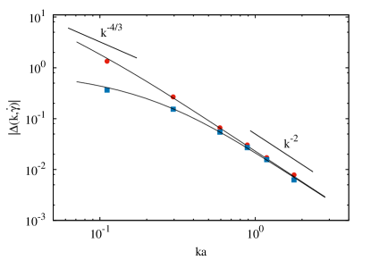
Figure 1: The nonequilibrium contribution to the transverse ($\Delta_{33}$, top) and longitudinal ($\Delta_{22}$, bottom) velocity correlations for $k_{x}=k_{y}$ and $k_{z}=0$. The lines correspond to the theoretical predictions given by Eqs. (17) and (18), and the symbols indicate simulation results. Parameters: $\dot{\gamma}=0.04\tau^{-1}$ and $h=0.1\tau$.

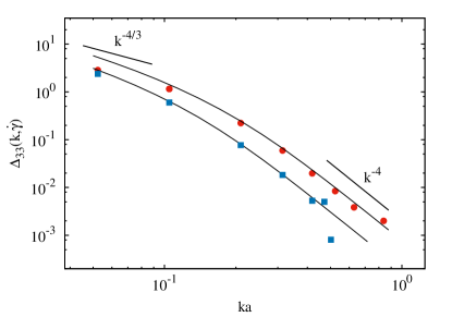
Figure 2: The nonequilibrium contribution to the transverse velocity ($\mathbf{e}^{(2)}$ direction) correlations for $k_{y}=k_{z}=0$. The line corresponds to the theoretical prediction as given in Eq. (18) and points represent the simulation data. Parameters: $h=0.2\tau$ and $\dot{\gamma}=0.02\tau^{-1}$ (top) and $\dot{\gamma}=0.01\tau^{-1}$ (bottom)

.

III Simulation approach

III.1 MPC simulations

In MPC simulations, the fluid is represented by point particles and their positions and velocities evolve in alternating discrete steps – streaming and collision. In the streaming, the particles moves ballistically, i.e., the positions are updated as

$$\mathbf{r}_{i}(t+h)=\mathbf{r}_{i}(t)+h\mathbf{v}_{i}(t),$$ (23)

where $h$ is the time step. In the collision, the particles are grouped into cubic cells of length $a$, and a stochastic rotation of the relative velocities, with respect to the center-of-mass velocity, of the particles is performed in each cell, i.e.,

$$\mathbf{v}_{i}(t+h)=\bm{v}_{cm}(t)+\mathcal{R}\left(\alpha\right)\left(\mathbf{v}_{i}(t)-\bm{v}_{cm}(t)\right)~{},$$ (24)

where

$$\bm{v}_{cm}=\frac{1}{N_{c}}\sum_{i\in\text{cell}}\mathbf{v}_{i}~{}.$$ (25)

Here, $N_{c}$ is the number of particles in the cell which contains particle $i$. $\mathcal{R}\left(\alpha\right)$ is the rotation matrix around a randomly oriented axis and $\alpha$ is the rotation angle Kapral (2008); Gompper et al. (2009). The shear flow is implemented by Lees-Edwards boundary conditions, in which the flow is generated by moving periodic simulation boxes by a velocity proportional to the boxes’ vertical position compared to the primary box Lees and Edwards (1972); Allen and Tildesley (1989). This boundary conditions is well suited for studying bulk properties of sheared fluids, as it eliminates finite size effects due to solid boundary walls. In order to maintain an isothermal state under shear, we employ a cell-level Maxwell-Boltzmann rescaling of the relative velocities of the particles Huang et al. (2010). This rescaling method for MPC fluid has been shown to reproduce the isothermal states consistent with the fluctuating Navier-Stokes equations in equilibrium and under shear flow Huang et al. (2012); Varghese et al. (2015).

Length- and time-scales in our simulations are given in terms of the length $a$ of a cubic cell and $\tau=\sqrt{ma^{2}/k_{B}T}$, where $m$ is the mass of a MPC fluid particle. The rotation angle $\alpha$ is chosen as $130^{\circ}$, the average number of fluid particles per cell as $\langle N_{c}\rangle=10$, and the time steps $h=0.1\tau$ and $0.2\tau$ are used. The length of the simulation box ranges from $L=20a$ to $120a$. The values of the transport coefficients for a given set of simulation parameters can be evaluated from theoretical expressions Tüzel et al. (2006); Gompper et al. (2009); Winkler and Huang (2009) and are given by $\nu=0.870a^{2}/\tau$ and $\tilde{\nu}=0.886a^{2}/\tau$ for $h=0.1\tau$, and $\nu=0.508a^{2}/\tau$ and $\tilde{\nu}=0.540a^{2}/\tau$ for $h=0.2\tau$.

III.2 Simulation results and discussion

In order to calculate the correlations in the simulations, the velocity field of the fluid in Fourier space is defined as

$$\delta\tilde{\mathbf{u}}(\mathbf{k})=\frac{m}{\rho_{0}}\sum_{i=1}^{N}[\mathbf{v}_{i}-\dot{\gamma}y_{i}\hat{\mathbf{x}}]e^{-i\mathbf{k}\cdot\mathbf{r}_{i}},$$ (26)

where $\rho_{0}=mN/V$ is the mean mass density and $V=L^{3}$. The mean flow is subtracted from the particle velocity, hence $\delta\tilde{\mathbf{u}}$ represents the thermally fluctuating part. The velocity correlation functions are then evaluated as

$$C_{ij}(\mathbf{k},\dot{\gamma})=V^{-1}\langle\delta\tilde{u}^{(i-1)}(\mathbf{k})\delta\tilde{u}^{(j-1)}(-\mathbf{k})\rangle~{},$$ (27)

where $i,j\in\{2,3,4\}$. $C_{22}$ corresponds to the longitudinal, and $C_{33}$ and $C_{44}$ to the transverse components. At equilibrium, i.e., $\dot{\gamma}=0$, the velocity correlation functions with velocity fields defined as in Eq. (26) are given by $C_{ii}=k_{B}T/\rho_{0}$ and $C_{ij}=0$ for $i\neq j$. In order to avoid $\mathcal{O}(N^{2})$ computational time in evaluating correlation functions in shear flow implemented by Lees-Edwards boundary conditions Lange (2009), the sampling is carried out at every $1/\dot{\gamma}$ time steps, at which the usual periodic boundary conditions apply ($\mathcal{O}(N)$ computational time).

III.2.1 Velocity fluctuations

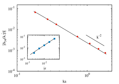
Figure 3: The coupling between the transverse velocity components for $k_{x}=k_{y}=k_{z}>0$. The inset shows the variation of the coupling with the shear rate for $k_{z}=2\pi/60$. The lines represent the theoretical predictions by Eq. (19) and the simulation data are represented by points. Parameters: $h=0.1\tau$ and $\dot{\gamma}=0.04\tau^{-1}$ for the main plot.

As is well known, the velocity fluctuations in a fluid at equilibrium are isotropic and spatially delta-correlated. Thus, in the Fourier-space representation, the correlations are independent of the wave vector $\mathbf{k}$. However, as is evident from Eqs. (17) and (18), the nonequilibrium contribution $\Delta_{ij}$ to the correlations in shear flow depends on the magnitude as well as the direction of the wave vector, thereby rendering the fluctuations spatially correlated and anisotropic. Figure 1 displays the nonequilibrium contributions of the longitudinal ($\mathbf{e}^{(1)}$ direction) and transverse ($\mathbf{e}^{(2)}$ direction) velocity correlations for a wave vector in the flow-gradient plane pointing at an angle $45^{\circ}$ to the flow direction. The correlations decay as $k^{-2}$ for large wave vectors. This power-law dependence for the transverse velocity correlations has been derived previously de Zárate and Sengers (2008).

Figure 2 displays the nonequilibrium enhancement of transverse velocity correlations for the wave vector pointing along the flow direction, i.e., $k_{y}=k_{z}=0$. As predicted by the theory, the correlations decay as $k^{-4}$ for large wave vectors. Since the $k^{-4}$ dependence corresponds to diverging correlations in real space, a slower decay is expected for smaller wave vectors. From the asymptotic analysis of the correlation functions, it was shown that the velocity correlations decay as $k^{-4/3}$ for small $k$ Wada and Sasa (2003); Wada (2004); de Zárate and Sengers (2008). This power-law dependence corresponds to a $r^{-5/3}$ decay in real space and is independent of the direction of the wave vector de Zárate and Sengers (2008). Unfortunately, we are not able to probe this small wave vector decay due to limitations in system size and shear rate in our simulations. However, it is clear from our simulation results that the velocity correlations indeed show a cross over from $k^{-4}$ (Fig. 2) and also $k^{-2}$ (Fig. 1) decay to a slower decay for small wave vectors. The agreement between the simulation results and the theoretical expressions for the wave vectors accessible for finite-system sizes strongly suggest that the correlations for infinite systems would indeed be long-ranged. It is noteworthy that rigid boundaries, which are absent in our simulations, is expected to modify the $k^{-4/3}$ small wave vector decay of the velocity correlations to a $k^{2}$ dependence de Zárate and Sengers (2008, 2009, 2006) .

The transverse components of the fluid-velocity field at equilibrium are well known to be identical and decoupled. Under shear, the degeneracy is lifted and the components become coupled Lutsko and Dufty (1985); Varghese et al. (2015). The strength of the coupling is given by Eq. (19). Figure 3 shows the variation of the coupling for the wave vector pointing out of the shear-gradient plane. The coupling decays as $k^{-2}$, corresponding to $r^{-1}$ decay, for the entire range of wave vectors in our simulations. In agreement with the theory, the coupling increases linearly with shear rate (cf. inset of Fig. 3). As is evident from Eq. (22), the coupling vanishes for wave vectors in the shear-gradient plane ($k_{z}=0$).

For large shear rates and small wave vectors, we observe deviations for the velocity correlations obtained by simulations and predicted theoretically (Fig. 2 top curve). We notice that a similar unexpected behavior was found for the large-length-scale decay of real-space correlations in sheared granular fluids Otsuki and Hayakawa (2009a). This effect may be attributed to a density dependence of the viscosity of the fluid. For fluids with density-dependent viscosity, the density fluctuations will be coupled to the mean flow velocity through an additional term in the linearized Navier-Stokes equation. This coupling is non-negligible for high shear rates and modify the eigenvalues and eigenvectors and thereby the hydrodynamic fluctuations. We hope to address this issue in detail in the future.

III.2.2 Density correlations

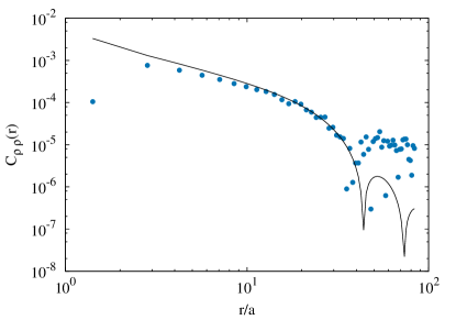
Figure 4: Spatial correlations in density fluctuations in shear flow. The line represents Eq. (29) and symbols simulation results. The correlations are measured in the shear-gradient plane and in the direction $45^{\circ}$ to the flow. Parameters: $h=0.2\tau$, $\dot{\gamma}=0.01\tau^{-1}$ and $L=120a$.

The density fluctuations, similar to the velocity fluctuations, become spatially correlated in shear flow. The correlation in the density fluctuations is defined as

$$C_{\rho\rho}(\mathbf{r})=\langle\delta\rho(\mathbf{r})\delta\rho(\mathbf{0})\rangle~{},$$ (28)

where $\delta\rho(\mathbf{r})=\rho(\mathbf{r})-\rho_{0}$. In simulations, the correlation is measured as $m^{2}\langle\delta n(\mathbf{r}_{0})\delta n(\mathbf{r}_{0}+\mathbf{r})\rangle$, where $n(\mathbf{r})$ is number of MPC particle in a given cell, with $\mathbf{r}_{0}$ and $\mathbf{r}$ taken as the centers of the cells. The theoretical expressions for $C_{\rho\rho}(\mathbf{r})$ can be obtained by inverting $C_{11}(\mathbf{k},\dot{\gamma})$ (see Eq. (15) and subsequent discussion), and is given by

$$C_{\rho\rho}(\mathbf{r})=\frac{m\rho_{0}}{V}\sum_{\mathbf{k}}\left[1+\Delta_{11}(\mathbf{k},\dot{\gamma})\right]\cos(\mathbf{k}\cdot\mathbf{r})~{},$$ (29)

where $\Delta_{11}(\mathbf{k},\dot{\gamma})$ is given by Eq. (17).

Figure 4 shows a comparison of the MPC simulation results for the density correlations and the numerically evaluated theoretical expression  (29). The agreement between the two results is good for moderate length scales. The deviation of the simulation results for small length scales is firstly due to the fact that the theoretical expression for the nonequilibrium contribution $\Delta_{11}(\mathbf{k},\dot{\gamma})$ is a good approximation for small wave vectors only. Secondly, the validity of Navier-Stokes equations for a MPC fluid breaks down at small length scales $r\lesssim\pi\sqrt{\nu h}$ Huang et al. (2012). One the other hand, for large length scales, the simulation data suffer from large statistical errors. However, for intermediate length scales, the correlations are well reproduced.

III.2.3 Pressure fluctuations

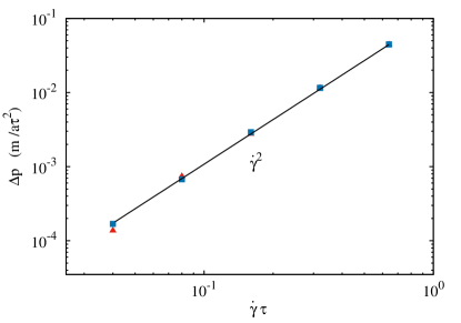
Figure 5: The nonequilibrium contribution to the pressure tensor (Eq. (30)), for the gradient (triangles) and vorticity (squares) components. Parameters: $L=60a$, $h=0.1\tau$.

The nonequilibrium contribution to the velocity correlations is also manifested in a shear-rate dependence of the pressure of the fluid Wada and Sasa (2003). The pressure in our simulations was measured as time average of the diagonal components of the instantaneous pressure tensor Winkler and Huang (2009)

$$p_{\alpha\beta}=\frac{m}{V}\sum_{i=1}^{N}\left[v_{i\alpha}v_{i\beta}+\frac{1}{h}\Delta v_{i\alpha}r_{i\beta}^{\prime}+\delta_{\alpha x}\delta_{\beta y}\frac{\dot{\gamma}h}{2}v_{iy}^{2}\right]$$ (30)

where ${\bm{v}}_{i}=\mathbf{v}_{i}-\dot{\gamma}y_{i}\hat{\mathbf{x}}$ is the thermal velocity after streaming, $\Delta\bm{v}_{i}$ is the change in the velocity in the collision step, and $\mathbf{r}_{i}^{\prime}$ is the position of the particle in the grid-shifted frame in the collision step. The pressure tensor for a MPC fluid at equilibrium is given by the ideal gas equation of state $p_{\alpha\beta}=\delta_{\alpha\beta}n_{0}k_{B}T$, where $n_{0}$ is the mean number density.

Figure 5 displays the deviation of the diagonal components of the pressure tensor from the equilibrium value. We observe that for high shear rates, the deviations vary as $\dot{\gamma}^{\zeta}$, with $\zeta=2$. The exponent $\zeta$ associated with the change in pressure has been controversial. Mode coupling theory Kawasaki and Gunton (1973) predicts $\zeta=3/2$, which has been confirmed in simulations of Lenard-Jones fluids at the triple point Evans (1981). However, in atom-scale simulations using two- and three-body potentials, the exponent was observed to be $\zeta\approx 2.0$ away from the triple point Marcelli et al. (2001a). The deviation was ascribed to two-body interactions Marcelli et al. (2001b); Ge et al. (2001). Further systematic studies using the Lenard-Jones potential found the exponent in the range $\zeta=1.2-2.0$ as a function of density and temperature Ge et al. (2003), thereby rendering $\zeta=3/2$ only a special case. Fluctuating hydrodynamic calculations of incompressible fluids on the other hand predict two limiting regimes of the variation of pressure, depending on the value of the dimensionless parameter $\lambda=\dot{\gamma}L^{2}/\nu$ Wada and Sasa (2003). The exponent is expected to be $\zeta=2$ for $\lambda\ll 1$ and $\zeta=3/2$ for $\lambda\gg 1$. However, our simulations yield $\zeta=2$ even for $\lambda\gg 1$, which is not a contradiction, as MPC fluid is highly compressible. It therefore remains for further theoretical and simulation studies to establish a unified picture of the exponent associated with the hydrostatic pressure under shear.

IV Conclusions

Using MPC simulations, we have unambiguously demonstrated that the hydrodynamic fluctuations in simple fluids under shear flow, in contrast to the fluctuations at equilibrium, are spatially correlated. The correlations in velocity and density fluctuations are shown to be anisotropic and spatially correlated over the entire volume of the system. For large wave vectors, the decay of the velocity correlations exhibits a power-law dependence in the wave vector. We observe a $k^{-4}$ decay for wave vector pointing along the flow direction and a $k^{-2}$ dominated decay along off-flow directions. For small wave vectors, we observe a cross-over to slower decay, indicating algebraic decay of real-space correlations at large distances. In contrast to the case at equilibrium, the transverse velocity components are coupled under shear, with a $k^{-2}$ dependence for the entire range of wave vectors accessible in our system, corresponding to $r^{-1}$ real space correlations. We find good agreement between the simulation results and the predictions of fluctuating hydrodynamics without any fitting parameters.

Although we have shown that the hydrodynamic fluctuations under shear are spatially correlated, it remains for further simulation studies to show they are truly long-ranged, i.e., for instance, that the transverse velocity fluctuations decay as $k^{-4/3}$ for small wave vectors. This demands either higher shear-rates or large system sizes than those accessible in our current study. Since MPC fluid is compressible with a density-dependent viscosity, large density fluctuations – although they are physical – arise under such conditions. Other hydrodynamic simulation methods for incompressible fluids, which incorporate thermal fluctuations, may therefore alternatively prove adequate.

We also find in our simulations that the nonequilibrium contribution to the hydrostatic pressure follows a $\dot{\gamma}^{2}$ dependency on shear rate, in contrast to the $\dot{\gamma}^{3/2}$ dependency predicted by mode-coupling theory. Our mesoscale simulation result is in agreement with the findings of previous atom-scale simulations studies using a range of interaction potentials, where deviation from the $\dot{\gamma}^{3/2}$ dependency was observed. A fundamental understanding of the hydrostatic pressure under shear is still lacking. The effect of confining walls on pressure and spatial correlations in hydrodynamic fluctuations are also yet to be addressed in simulations.

References

- Boon and Yip (1980) J. P. Boon and S. Yip, Molecular hydrodynamics (Courier Corporation, 1980).
- Hansen and McDonald (1990) J.-P. Hansen and I. R. McDonald, Theory of simple liquids (Elsevier, 1990).
- De Zarate and Sengers (2006) J. M. O. De Zarate and J. V. Sengers, Hydrodynamic fluctuations in fluids and fluid mixtures (Elsevier, 2006).
- Kirkpatrick et al. (1980) T. Kirkpatrick, E. G. D. Cohen, and J. R. Dorfman, Phys. Rev. Lett. 44, 472 (1980).
- Ronis and Procaccia (1982) D. Ronis and I. Procaccia, Phys. Rev. A 26, 1812 (1982).
- Law et al. (1988) B. M. Law, R. W. Gammon, and J. V. Sengers, Phys. Rev. Lett. 60, 1554 (1988).
- Segrè et al. (1992) P. N. Segrè, R. W. Gammon, J. V. Sengers, and B. M. Law, Phys. Rev. A 45, 714 (1992).
- Lutsko and Dufty (1985) J. Lutsko and J. W. Dufty, Phys. Rev. A 32, 3040 (1985).
- Wada and Sasa (2003) H. Wada and S.-I. Sasa, Phys. Rev. E 67, 065302 (2003).
- de Zárate and Sengers (2008) J. M. O. de Zárate and J. V. Sengers, Phys. Rev. E 77, 026306 (2008).
- de Zárate and Sengers (2009) J. M. O. de Zárate and J. V. Sengers, Phys. Rev. E 79, 046308 (2009).
- Otsuki and Hayakawa (2009a) M. Otsuki and H. Hayakawa, Phys. Rev. E 79, 021502 (2009a).
- Otsuki and Hayakawa (2009b) M. Otsuki and H. Hayakawa, Eur. Phys. J. Special Topics 179, 179 (2009b).
- Varghese et al. (2015) A. Varghese, C.-C. Huang, R. G. Winkler, and G. Gompper, Phys. Rev. E 92, 053002 (2015).
- de Zárate and Sengers (2004) J. M. O. de Zárate and J. V. Sengers, J. Stat. Phys. 115, 1341 (2004).
- de Zárate and Sengers (2011) J. M. O. de Zárate and J. V. Sengers, J. Stat. Phys. 144, 774 (2011).
- de Zárate and Sengers (2013) J. M. O. de Zárate and J. V. Sengers, J. Stat. Phys. 150, 540 (2013).
- Kapral (2008) R. Kapral, Adv. Chem. Phys. 140, 89 (2008).
- Gompper et al. (2009) G. Gompper, T. Ihle, D. M. Kroll, and R. G. Winkler, Adv. Polym. Sci. 221, 1 (2009).
- Pooley and Yeomans (2005) C. M. Pooley and J. M. Yeomans, J. Phys. Chem. B 109, 6505 (2005).
- Winkler and Huang (2009) R. G. Winkler and C.-C. Huang, J. Chem. Phys. 130, 074907 (2009).
- Híjar and Sutmann (2011) H. Híjar and G. Sutmann, Phys. Rev. E 83, 046708 (2011).
- Huang et al. (2015) C.-C. Huang, A. Varghese, G. Gompper, and R. G. Winkler, Phys. Rev. E 91, 013310 (2015).
- Landau and Lifshitz (1987) L. D. Landau and E. M. Lifshitz, Fluid mechanics, Vol. 6 (Elsevier, 1987).
- Huang et al. (2012) C.-C. Huang, G. Gompper, and R. G. Winkler, Phys. Rev. E 86, 056711 (2012).
- Wada (2004) H. Wada, Phys. Rev. E 69, 031202 (2004).
- Lees and Edwards (1972) A. W. Lees and S. F. Edwards, J. Phys. C 5, 1921 (1972).
- Allen and Tildesley (1989) M. P. Allen and D. J. Tildesley, Computer simulation of liquids (Oxford, 1989).
- Huang et al. (2010) C.-C. Huang, A. Chatterji, G. Sutmann, G. Gompper, and R. G. Winkler, J. Comp. Phys. 229, 168 (2010).
- Tüzel et al. (2006) E. Tüzel, T. Ihle, and D. M. Kroll, Phys. Rev. E 74, 056702 (2006).
- Lange (2009) E. Lange, Brownian dynamics analysis of dense dispersions under shear, Ph.D. thesis, Konstanz, Univ. (2009).
- de Zárate and Sengers (2006) J. M. O. de Zárate and J. V. Sengers, Phys. Rev. E 73, 013201 (2006).
- Kawasaki and Gunton (1973) K. Kawasaki and J. D. Gunton, Phys. Rev. A 8, 2048 (1973).
- Evans (1981) D. J. Evans, Phys. Rev. A 23, 1988 (1981).
- Marcelli et al. (2001a) G. Marcelli, B. D. Todd, and R. J. Sadus, Phys. Rev. E 63, 021204 (2001a).
- Marcelli et al. (2001b) G. Marcelli, B. D. Todd, and R. J. Sadus, Fluid Phase Equilib. 183, 371 (2001b).
- Ge et al. (2001) J. Ge, G. Marcelli, B. D. Todd, and R. J. Sadus, Phys. Rev. E 64, 021201 (2001).
- Ge et al. (2003) J. Ge, B. D. Todd, G. Wu, and R. J. Sadus, Phys. Rev. E 67, 061201 (2003).