Static spherically symmetric wormholes in generalized $f(R,\phi)$ gravity

Abstract

In this paper, we examine static spherically symmetric wormhole solutions in generalized $f(R,\phi)$ gravity. To do this, we consider three different kinds of fluids: anisotropic, barotropic and isotropic. We explore different $f(R,\phi)$ models and inspect the energy conditions for all of those three fluids. It is found that under some models in this theory, it is possible to obtain wormhole solutions without requiring exotic matter. The discussion about the conditions where the standard energy conditions (WEC and NEC) are valid for the fluids is discussed in details. From our results and for our cases, we conclude that for anisotropic and isotropic fluids, realistic wormhole geometries satisfying the energy conditions can be constructed.

1 Introduction

From theoretical and observational reasons, it is believed that General Relativity (GR) might be an incomplete theory. During the last few decades, considerable efforts have been made to formulate alternative theories of gravity. In this perspective, scalar-tensor gravity theory appeared as one of the most popular candidates. In 1955, Jordan proposed a complete gravitational theory based on the idea that $G$ (the gravitational constant in GR) plays the role of a gravitational scalar field in accordance with Dirac’s argument in such a way that the gravitational constant should be time-dependent 5 ; 1* . In 1961, Brans and Dicke presented a scalar-tensor gravity theory as an effort to incorporate the Mach’s proposal in the Einstein-Hilbert gravitational framework, the so-called Brans-Dicke (BD) theory 6 . This theory has been generalized in different ways, for example by introducing some arbitrary potential functions for the scalar field 2* , or considering a field$-$dependent BD parameter 3* or introducing inverse curvature correction in BD action 4* or considering a non-minimal coupling between the scalar field and matter systems (chameleonic BD gravity) 5* .

Quintessence scalar-tensor theory is one of the minimally coupled theories whose Lagrangian is the sum of Einstein-Hilbert Lagrangian plus a contribution from the scalar field. Non-minimal couplings (NMC) between the scalar field and the scalar curvature $R$ introduce an additional term of the form $f(\phi)R$ (where $f(\phi)$ is a function of the scalar field $\phi$) in the Lagrangian of quintessence models 6* . NMC models have been employed to discuss various cosmological issues such as: scaling attractor solutions which can provide accelerated cosmic expansion at the present time 7* , oscillating universe 8* , reconcile cosmic strings production with inflation 9* , discuss the phase space analysis 10* , model a modified Newtonian dynamics able to model flat rotation curves in galaxies 11* , discuss some cosmological constraints on weak gravitational lensing in such theories 12* and others. In 13* , authors discussed cosmological perturbations and reconstruction method in a generalized scalar-tensor theory, which is an extended form of $Rf(\phi)$ gravity, with the following Lagrangian

$$\mathcal{L}=\frac{1}{\kappa^{2}}\left(f(R,\phi)+\omega(\phi)\,\phi_{;\alpha}\,\phi^{;\alpha}\right)+V(\phi)\,,$$

where now $f(R,\phi)$ depends on both $R$ and the scalar field $\phi$, $V(\phi)$ is the energy potential and $w(\phi)$ is the Brans-Dicke function which in general depends on $\phi$. Here, semicolon represents covariant differentiation, so that $\phi_{;\alpha}=\nabla_{\alpha}\phi$. From this Lagrangian (sometimes called extended quintessence), many different scalar-tensor theories can be recovered as special cases. In this extended quintessence theory, various aspects have been discussed, for example: search of a vacuum energy that can be a possible explanation of the data from high-redshift type-Ia supernovae 14* , cosmological evolution in the presence of exponential couplings 15* , study of structure formation based on NMC models 16* , cosmological perturbations of such models in the metric and Palatini formalisms 17* , non-linear structure formation in cosmological models using the method of spherical collapse 18* , among other studies.

Wormholes are hypothetical topological objects that provide a shortcut connecting two distant regions in a space-time or bridging two distinct universes. The study of such geometrical objects started in 1916 by Flamm 7 and then followed by the work of Einstein and Rosen in 1935 8 . In the latter work, they found a space-time solution whose geometry consists in two mouths and a throat known as an Einstein-Rosen bridge. Misner and Wheeler introduced the word “wormhole” for such objects in 1957 9 . They also showed that wormholes cannot be traversable for standard matter due to its instability. The current interest in wormholes started after the important works done by Morris and Thorne and Yurtsever 10 . They formally presented a metric, the so-called Morris-Thorne metric, and give some conditions in order to have a traversable wormhole. They showed that wormholes can be traversable provided that they are supported by exotic matter, which involves a stress energy tensor that violates the null energy condition (NEC). There already exists an important number of works exploring the possible existence of wormhole geometries in different physical situations. In the literature, some attempts have been made to reduce the impact of exotic matter and minimize the violation of energy conditions 11 . One interesting approach is the one made by alternatives theories of gravity. The main idea of this approach lies on assuming that the matter which supports the wormhole does not violate the energy conditions but all the new terms coming from the theory produces this violation 22* ; 23* ; 24* . The procedure is the following. In all of those modified theories, it is possible to rewrite the field equations using effective fluids defined as the sum of the standard fluid plus a new fluid which represents all the new terms coming from the modified theory. Then, one can impose that the standard matter fluid satisfies the energy conditions (NEC and WEC) but the effective fluids do not. Hence, one can say that those new terms coming from modified gravity are the responsible of the violation of the standard energy needed to support a traversable wormhole. Wormhole solutions have been constructed in various modified theories such as $f(R)$ gravity 22* , $f(T)$ gravity 23* , $f(R,\mathcal{T})$ gravity (where $\mathcal{T}$ is the trace of the energy-momentum tensor) 24* , BD theory 25* -28* , metric-Palatini hybrid $f(R)$ 29* , scalar-tensor teleparallel gravity 30* , in Einstein-Gauss-Bonnet gravity 31* and in others.

In 25* , Agnese and Camera found static spherically symmetric solutions in BD theory which can describe wormhole solutions depending on the choice of post Newtonian parameter $\gamma>1$. BD theory could admit traversable wormhole solutions for both positive and negative values of BD parameter ($\omega<-2$ and $\omega<\infty$). In this study, the scalar field plays the role of the exotic matter 26* ; 27* . Ebrahimi and Riazi 28* used a traceless energy momentum to find two classes of Lorentizan wormhole solutions in BD theory. The first one was obtained in a open universe whereas the second wormhole solution was obtained for both open and closed universes. However, the WEC is violated for these solutions. The existence of Euclidean wormhole solutions has also been explored in BD theory and Induced Gravity 32* .

In this paper, we are interested to explore the existence of traversable wormhole geometries in the extended quintessence scalar-tensor theory given by the Lagrangian (1). We will study the conditions where the energy conditions are satisfied for three different types of fluids: anisotropic, isotropic and barotropic fluids. In the case of the anisotropic fluid, we will specify the shape function to then find the appropriate regions where the wormhole solutions exist. In the other cases (isotropic and barotropic fluids), the shape function will be analytically and numerically found from the field equations. This paper is organised as follows: Sec. 2 is devoted to present the field equations for the Morris-Thorne metric in our extended quintessence scalar-tensor theory. Additionally, in this section we will find the general energy conditions for the modified equations under this geometry. In Sec. 3, we study in detail the validity of the energy conditions for anisotropic fluid by assuming an specific shape function. Secs. 4 and 5 are devoted to find and study analytical wormholes solutions for the isotropic and barotropic fluid respectively. Finally, in Sec. 6 we summarize our main results.

2 Wormhole Geometries in extended $f(R,\phi)$ Gravity

In this section we will present the field equations for the extended $f(R,\phi)$ gravity in the Morris-Thorne geometry and then study its generic properties to find out the general energy conditions. The extended $f(R,\phi)$ theory is constructed with the Lagrangian (1) in such a way that its action takes the following form 19* ,

$$S=\int d^{4}x\sqrt{-g}\left[\frac{1}{\kappa^{2}}\left(f\left(R,\phi\right)+\omega(\phi)\,\phi_{;\alpha}\,\phi^{;\alpha}\right)+V(\phi)\right]+S_{m}\,,$$ (2.1)

where $\kappa^{2}=8\pi G$ and $S_{m}$ represents the action of the matter. By varying the above action with respect to the metric, we find the following field equations,

$$f_{R}\,R_{\mu\nu}-\frac{1}{2}\left(f+\omega(\phi)\,\phi_{;\alpha}\,\phi^{;\alpha}\right)\,g_{\mu\nu}-f_{R;\mu\nu}+g_{\mu\nu}\,\Box f_{R}+\omega(\phi)\,\phi_{;\mu}\,\phi_{;\nu}+g_{\mu\nu}V(\phi)=\kappa^{2}\,T_{\mu\nu}\,,$$ (2.2)

where $\Box=g^{\mu\nu}\nabla_{\mu}\nabla_{\nu}$, $f_{R}=\partial f/\partial R$ and $T_{\mu\nu}=\delta S_{m}/\delta g^{\mu\nu}$ is the energy-momentum tensor. Additionally, by taking variations in (2.1) with respect to the scalar field we find the modified Klein-Gordon equation,

$$2\,\omega(\phi)\,\Box\phi+\omega_{\phi}(\phi)\,\phi_{;\alpha}\,\phi^{;\alpha}-f_{\phi}+V_{\phi}(\phi)=0\,.$$ (2.3)

We can rewrite the field equation (2.2) in an effective form,

$$G_{\mu\nu}=R_{\mu\nu}-\frac{1}{2}Rg_{\mu\nu}=T_{\mu\nu}^{\rm eff}\,,$$ (2.4)

where $T_{\mu\nu}^{\rm eff}$ is the effective energy-momentum tensor defined as

$$T_{\mu\nu}^{\rm eff}=\frac{1}{f_{R}}\bigg{[}\kappa^{2}T_{\mu\nu}+\frac{1}{2}\left(f+\omega(\phi)\phi_{;\alpha}\phi^{;\alpha}-Rf_{R}\right)g_{\mu\nu}+f_{R;\mu\nu}-g_{\mu\nu}\Box f_{R}-\omega(\phi)\phi_{;\mu}\phi_{;\nu}-g_{\mu\nu}V(\phi)~{}\bigg{]}\,.$$ (2.5)

The metric which could describes static spherically symmetric wormholes is the Morris-Thorne metric which can be written as 10

$$ds^{2}=e^{a(r)}dt^{2}-e^{b(r)}dr^{2}-r^{2}(d\theta^{2}+\sin^{2}\theta d\phi^{2})\,,$$ (2.6)

where $a(r)$ represents the redshift function which depends on the radial coordinate $r$ and $b(r)$ is a function which related to the shape function $\beta(r)$ via

$$e^{-b(r)}=1-\frac{\beta(r)}{r}\,.$$ (2.7)

The shape function must satisfy the condition that at the throat $r_{0}$ is equal to $\beta(r=r_{0})=r_{0}$ and then it must increases from $r_{0}$ to $\infty$. For the existence of standard wormholes, the shape function must also satisfy the flaring-out condition which reads

$$\frac{\beta(r)-\beta^{\prime}(r)r}{\beta(r)^{2}}>0\,,\ \ \ \textrm{at}\ \ r=r_{0}\,.$$ (2.8)

The above condition can be also written in a short way, namely $\beta^{\prime}(r=r_{0})<1$. In addition, to do not change the signature of the metric, the shape function must also satisfy the condition $1-\beta(r)/r>0$.
Since we are interested on studying wormhole geometries for anisotropic, isotropic and barotropic fluids, we will first derive the equation for the most general of those fluids, i.e., the anisotropic fluid. Then, when it is necessary, the other particular cases (barotropic and isotropic) can be easily recovered. For an anisotropic fluid, the energy-momentum tensor is defined as follows

$$T_{\mu\nu}=(\rho+p_{t})V_{\mu}V_{\nu}-p_{t}g_{\mu\nu}+(p_{r}-p_{t})X_{\mu}X_{\nu}\,,$$ (2.9)

where $\rho$, $p_{r}$ and $p_{t}$ are the energy density, radial pressure and lateral pressure of the fluid respectively measured in the orthogonal direction of the unit space-like vector in the radial vector $X_{\mu}=e^{-b}\delta^{\mu}_{1}$. Additionally, $V_{\mu}=e^{-a}\delta^{\mu}_{0}$ is the 4-velocity which satisfies the conditions $V^{\mu}V_{\mu}=1$, $X^{\mu}X_{\mu}=-1$ and also $X^{\mu}V_{\mu}=0$.
If we consider the above energy-momentum tensor and the Morris-Thorne metric (2.6), the generalized $f(R,\phi)$ field equations given by (2.2) become

$$\kappa^{2}\rho = -e^{-b}f_{R}^{\prime\prime}+\frac{1}{2r}e^{-b}\left(rb^{\prime}+4\right)f_{R}^{\prime}+\frac{1}{4r}e^{-b}\left(2ra^{\prime\prime}+r{a^{\prime}}^{2}-ra^{\prime}b^{\prime}+4a^{\prime}\right)f_{R}$$ (2.10)

$$+\frac{1}{2}\omega(\phi)e^{-b}{\phi^{\prime}}^{2}-\frac{1}{2}f+V(\phi)\,,$$

$$\kappa^{2}p_{r} = \frac{1}{2r}e^{-b}\left(ra^{\prime}+4\right)f_{R}^{\prime}-\frac{1}{4r}e^{-b}\left(2ra^{\prime\prime}+r{a^{\prime}}^{2}-ra^{\prime}b^{\prime}-4b^{\prime}\right)f_{R}$$ (2.11)

$$-\frac{1}{2}e^{-b}\omega(\phi){\phi^{\prime}}^{2}+\frac{1}{2}f-V(\phi)\,,$$

$$\kappa^{2}p_{t} = e^{-b}f_{R}^{\prime\prime}+\frac{1}{2r}e^{-b}\left(ra^{\prime}-rb^{\prime}+2\right)f_{R}^{\prime}+\frac{1}{2r^{2}}e^{-b}\left(rb^{\prime}-ra^{\prime}+2e^{b}-2\right)f_{R}$$ (2.12)

$$-\frac{1}{2}e^{-b}\omega(\phi){\phi^{\prime}}^{2}+\frac{1}{2}f-V(\phi)\,,$$

where primes denote differentiation with respect to the radial coordinate $r$. In GR, wormhole geometries are supported by exotic matter which requires the violation of NEC and WEC. In 20 , Harko et al. discussed wormholes in modified theories and showed that these geometries can be theoretically constructed without the presence of exotic matter. In such scenario, matter threading a wormhole satisfies the energy conditions and the additional geometric components coming from the modified theory are the responsible of the violation of the energy conditions. Hence, the violation of the NEC and WEC are described in terms of the effective energy momentum tensor, i.e.,

$$\textrm{WEC}:\ W^{\mu}W^{\nu}T_{\mu\nu}^{\rm eff}<0\,,\quad\textrm{NEC}:k^{\mu}k^{\nu}T_{\mu\nu}^{\rm eff}<0\,,$$ (2.13)

for any $W^{\mu}$ time-like vector and any $k^{\mu}$ null-like vector. By doing that, we can then impose that the matter satisfies those conditions:

$$\textrm{WEC}:W^{\mu}W^{\nu}T_{\mu\nu}>0\,,\quad\textrm{NEC}:k^{\mu}k^{\nu}T_{\mu\nu}>0\,.$$ (2.14)

Clearly, if NEC is violated then WEC will be also violated and if WEC is valid, it does not imply that the NEC is satisfied. In the literature, this approach has been discussed in different contexts including $f(R)$ gravity 22* , curvature-matter couplings 21 , braneworlds 22 , $f(T)$ theory 23* , or in hybrid metric-Palatini $f(R)$ 29* .
Applying the flaring out condition (2.8), one directly notice that NEC needs to be violated for the effective fluid. Hence, to have traversable wormhole geometries we have must impose the conditions $\rho^{\rm eff}+p_{r}^{\rm eff}<0$ and $\rho^{\rm eff}+p_{t}^{\rm eff}<0$. As we discussed above, those conditions do not imply that the standard matter violates NEC. Thus, we can then impose $\rho+p_{r}>0$ and $\rho+p_{t}>0$ to ensure that the matter satisfies the NEC, which gives us

$$\rho+p_{r} = -e^{-b}f^{\prime\prime}_{R}+\frac{1}{2r}e^{-b}\Big{(}r(a^{\prime}+b^{\prime})+8\Big{)}f^{\prime}_{R}+\frac{1}{r}e^{-b}(a^{\prime}+b^{\prime})f_{R}>0\,,$$ (2.15)

$$\rho+p_{t} = \frac{1}{2r}e^{-b}(ra^{\prime}+6)f^{\prime}_{R}+\frac{e^{-b}}{4r^{2}}\Big{[}2r^{2}a^{\prime\prime}+ra^{\prime}\left(2-rb^{\prime}\right)+r^{2}a^{\prime 2}+2rb^{\prime}+4e^{b}-4\Big{]}f_{R}>0\,.$$ (2.16)

Let us clarify that WEC will be valid if the above conditions are true and also assuming that the energy condition is always positive $\rho>0$. Thus, for the validity of WEC, we also need to impose that the right hand side in Eq. (2.10) is always positive. For the specific case where there are not tidal forces, i.e., when $a^{\prime}(r)=0$, the above conditions become

$$\rho+p_{r} = -e^{-b}f^{\prime\prime}_{R}+\frac{1}{2r}e^{-b}\Big{(}rb^{\prime}+8\Big{)}f^{\prime}_{R}+\frac{b^{\prime}}{r}e^{-b}f_{R}>0\,,$$ (2.17)

$$\rho+p_{t} = \frac{3}{r}e^{-b}f^{\prime}_{R}+\frac{e^{-b}}{4r^{2}}\Big{[}2rb^{\prime}+4e^{b}-4\Big{]}f_{R}>0\,.$$ (2.18)

Hereafter, we will consider $f(R,\phi)$ models given in a power-law way given by 20*

$$f(R,\phi)=\gamma R\phi^{n},$$ (2.19)

where $\gamma$ and $n$ are constants. Using this model, the field equations become

$$2\kappa^{2}\rho = \frac{\gamma^{2}e^{-3b}}{16r^{3}}\omega(\phi){\phi^{\prime}}^{2}\phi^{2n}\Big{(}2ra^{\prime\prime}-ra^{\prime}b^{\prime}+ra^{\prime 2}+4a^{\prime}\Big{)}\Big{(}-2r^{2}a^{\prime\prime}+r^{2}a^{\prime}b^{\prime}-r^{2}a^{\prime 2}-4ra^{\prime}+4rb^{\prime}$$ (2.20)

$$+ 4e^{b}-4\Big{)}+\frac{n\gamma e^{-b}}{r}\Big{(}rb^{\prime}+4\Big{)}\phi^{\prime}\phi^{n-1}-2n\gamma e^{-b}\phi^{\prime\prime}\phi^{n-1}-2\gamma n(n-1)e^{-b}\phi^{\prime 2}\phi^{n-2}$$

$$+ 2\kappa^{2}V(\phi)\,,$$

$$2\kappa^{2}p_{r} = \frac{n\gamma e^{-b}}{r}\left(ra^{\prime}+4\right)\phi^{\prime}\phi^{n-1}-\frac{\gamma e^{-b}}{2r^{2}}\left(-2r^{2}a^{\prime\prime}+r^{2}a^{\prime}b^{\prime}-r^{2}a^{\prime 2}-4ra^{\prime}+4rb^{\prime}+4e^{b}-4\right)\phi^{n}$$ (2.21)

$$- e^{-b}\omega(\phi)\phi^{\prime 2}-\frac{\gamma e^{-b}}{2r}\left(2ra^{\prime\prime}-ra^{\prime}b^{\prime}+ra^{\prime 2}-4b^{\prime}\right)\phi^{n}-2\kappa^{2}V(\phi)\,,$$

$$2\kappa^{2}p_{t} = \frac{\gamma e^{-b}}{r^{2}}\left(-ra^{\prime}+rb^{\prime}+2e^{b}-2\right)\phi^{n}+\frac{n\gamma e^{-b}}{r}\left(ra^{\prime}-rb^{\prime}+2\right)\phi^{\prime}\phi^{n-1}+2n\gamma e^{-b}\phi^{\prime\prime}\phi^{n-1}$$ (2.22)

$$- \frac{\gamma e^{-b}}{2r^{2}}\left(-2r^{2}a^{\prime\prime}+r^{2}a^{\prime}b^{\prime}-r^{2}a^{\prime 2}-4ra^{\prime}+4rb^{\prime}+4e^{b}-4\right)\phi^{n}+2\gamma n(n-1)e^{-b}\phi^{\prime 2}\phi^{n-2}$$

$$- e^{-b}\omega(\phi)\phi^{\prime 2}-2\kappa^{2}V(\phi)\,.$$

Now, if we replace (2.19) into (2.3) we get

$$\frac{dV}{d\phi} = -\frac{n\gamma e^{-b}}{2r^{2}}\left\{-2r^{2}a^{\prime\prime}+r^{2}a^{\prime}b^{\prime}-r^{2}a^{\prime 2}-4ra^{\prime}+4rb^{\prime}+4e^{b}-4\right\}\phi^{n-1}+e^{-b}\frac{d\omega}{d\phi}\phi^{\prime 2}+2\omega(\phi)e^{-b}$$ (2.23)

$$\times \left\{\phi^{\prime\prime}+\left(\frac{a^{\prime}-b^{\prime}}{2}+\frac{2}{r}\right)\phi^{\prime}\right\}\,.$$

Additionally, we will assume the following power-law functions for the BD function 25 and the scalar field 26

$$\omega(\phi)=\omega_{0}\phi^{m}\,,\quad\phi(r)=\phi_{0}\left(\frac{d}{r}\right)^{\sigma_{1}}\,,$$ (2.24)

where $a_{0}$, $d$ and $\omega_{0}$ are constants.

3 Anisotropic generic fluid description

This section is devoted to study wormholes supported by an anisotropic fluid characterized by $\rho$, $p_{r}$ and $p_{t}$ without specifying any equation of state. Our principal aim is to check the validity of the energy conditions (WEC and NEC) for our model. To do this, we will specify the $b(r)$ radial function as follows 23* ; 29 ; 30 ; 31 ; 32 ; 33 ; 34

$$b(r)=-\ln\left[1-\left(\frac{r_{0}}{r}\right)^{\sigma_{2}+1}\right]\,,$$ (3.1)

where $\sigma_{2}$ is a constant and $r_{0}$ is the throat of the wormhole, which gives us that the shape function is

$$\beta(r)=r_{0}\Big{(}\frac{r_{0}}{r}\Big{)}^{\sigma_{2}}\,.$$ (3.2)

This kind of shape function has been used widely in the literature and satisfies all the conditions needed to have a wormhole geometry if $\sigma_{2}>-1$ (see the flaring-out condition given by (2.8)). Table 1 shows the values that the shape function takes for different constants $\sigma_{2}$.

Table 1: Some shape functions for different values of the parameter $\sigma_{2}$

$\sigma_{2}$	$\sigma_{2}=1$	$\sigma_{2}=1/2$	$\sigma_{2}=1/5$	$\sigma_{2}=0$	$\sigma_{2}=-1/2$
Shape function $\beta(r)$	${r_{0}}^{2}/r$	$r_{0}\sqrt{r_{0}/r}$	${r_{0}}^{6/5}{r}^{-1/5}$	$r_{0}$	$\sqrt{r_{0}r}$

Additionally, for this section we will also assume that the redshift function is constant ($a^{\prime}(r)=0$), or in other words, we will assume zero tidal forces. Using power-law ansatz with model (2.19) and radial function (3.1) into (2.23) and integrating we have scalar potential of the form

$$V(\phi) = \frac{n\gamma{r_{0}}^{\sigma_{2}+1}{\sigma_{1}}(\sigma_{2}-3)\phi^{n+\frac{\sigma_{2}+3}{\sigma_{1}}}}{2d^{\sigma_{2}+3}{\phi_{0}}^{\frac{\sigma_{2}+3}{\sigma_{1}}}(n\sigma_{1}+\sigma_{2}+3)}-\frac{\omega_{0}m{\sigma_{1}}^{3}\phi^{m+2+\frac{1}{\sigma_{1}}}}{d^{2}{\phi_{0}}^{2/\sigma_{1}}(m\sigma_{1}+2\sigma_{1}+1)}+\frac{\omega_{0}m{\sigma_{1}}^{3}{r_{0}}^{\sigma_{2}+1}\phi^{m+2+\frac{\sigma_{2}+2}{\sigma_{1}}}}{d^{\sigma_{2}+3}{\phi_{0}}^{\frac{\sigma_{2}+3}{\sigma_{1}}}(m\sigma_{1}+2\sigma_{1}+\sigma_{2}+2)}$$ (3.3)

$$+ \frac{\omega_{0}{\sigma_{1}}^{2}(2\sigma_{1}-m\sigma_{1}-2)\phi^{m+2+\frac{2}{\sigma_{1}}}}{d^{2}{\phi_{0}}^{2/\sigma_{1}}(m\sigma_{1}+2\sigma_{1}+2)}+\frac{\omega_{0}{\sigma_{1}}^{2}{r_{0}}^{\sigma_{2}+1}(m\sigma_{1}-\sigma_{2}+3)\phi^{m+2+\frac{\sigma_{2}+3}{\sigma_{1}}}}{d^{\sigma_{2}+3}{\phi_{0}}^{\frac{\sigma_{2}+3}{\sigma_{1}}}(m\sigma_{1}+2\sigma_{1}+\sigma_{2}+3)}+c_{0}\,.$$

Here, $c_{0}$ is an integration constant. It should be noted that the special cases $n\sigma_{1}+\sigma_{2}+3=0,m\sigma_{1}+2\sigma_{1}+1=0,m\sigma_{1}+2\sigma_{1}+\sigma_{2}+2=0,m\sigma_{1}+2\sigma_{1}+2=0$ and $m\sigma_{1}+2\sigma_{1}+\sigma_{2}+3=0$ will be excluded from our analysis. In the following discussion, we will study the validity of WEC and NEC for the standard matter (see Eqs. (2.15) and (2.16)). Let us then study different different cases for $\sigma_{2}$ to study the validity of the energy conditions. To do this, we will fix $r_{0}=\phi_{0}=d=\omega_{0}=1$ and $\kappa^{2}=8\pi$ for simplicity. Additionally, it can be noticed from the equations that the constant $\gamma$ which appears from the model (see (2.19)) only will change the behaviour of the wormhole depending on its sign. Hence, we will study mainly two cases for this parameter, namely, when $\gamma=1$ and $\gamma=-1$. Let us also divide our study into two main theories: Brans-Dicke and Induced Gravity.

3.1 Brans-Dicke theory

To recover the case of Brans-Dicke theory we need to choose $n=1$ with $m=-1$. Now, we will discuss the validity of the energy conditions for the remaining parameters $\gamma$, $\sigma_{1}$ and $\sigma_{2}$. As we have pointed out before, only the sign of $\gamma$ changes the physical motion of the wormholes so we will set either $\gamma=1$ and $\gamma=-1$. Since we have two free parameter ($\sigma_{1}$ and $\sigma_{2}$), we will make region plots to check the validity of all the important energy conditions. For this model we have that the corresponding energy conditions are

$$\rho = \frac{(2\gamma-1)\sigma_{1}^{2}}{\gamma}+\frac{8\pi\sigma_{1}(\gamma(\sigma_{2}-3)-2\sigma_{1}(\sigma_{1}+\sigma_{2}-3))}{\gamma(\sigma_{1}+\sigma_{2}+3)}+\frac{16\pi\sigma_{1}^{3}r^{\sigma_{2}+2}}{\gamma\sigma_{1}+\gamma}+\frac{16\pi r^{\sigma_{1}+\sigma_{2}+3}}{\gamma}$$ (3.4)

$$+\frac{\sigma_{1}\left(\sigma_{1}(\sigma_{1}+16\pi(3\sigma_{1}-2)+2)-2\gamma\left(\sigma_{1}^{2}+5\sigma_{1}+6\right)\right)r^{\sigma_{2}+1}}{\gamma(\sigma_{1}+2)}-\frac{16\pi r\sigma_{1}^{3}}{\gamma(\sigma_{1}+\sigma_{2}+2)}$$

$$+\sigma_{1}\sigma_{2}+7\sigma_{1}-2\sigma_{2}\geq 0\,,$$

$$\rho+p_{r} = -2\sigma_{1}(\sigma_{1}+5)r^{\sigma_{2}+1}+2\sigma_{1}^{2}+\sigma_{1}(\sigma_{2}+11)-2(\sigma_{2}+1)\geq 0\,,$$ (3.5)

$$\rho+p_{t} = -6\sigma_{1}r^{\sigma_{2}+1}+6\sigma_{1}-\sigma_{2}+1\geq 0\,.$$ (3.6)

We can see that it is not so easy to check the validity of the energy conditions. Let us first study the case where $\sigma_{2}=1$ to visualise better the behaviour of the energy conditions. In that case, we are able to create 2D region plots for the validity of the energy conditions. Fig. 1 shows the validity of $\rho\geq 0$ (see (3.4)) for different values of $\sigma_{1}$ and $\gamma=1$ or $\gamma=-1$. Each blue(yellow) regions represent the validity of this condition for $\gamma=-1$($\gamma=1$). The green regions are the intersection regions where this condition is valid for $\gamma=1$ and $\gamma=-1$. As we can see from the figure, there is not so much difference in the valid region for positive or negative values of $\gamma$. However, one can directly see that for the region where $-2\lesssim\sigma_{1}\lesssim-1.3$, the condition $\rho>0$ will be never true. For other values, one can notice that the validity of this condition depends on the location of the observer. For an observer who is far away from the throat (located at $r_{0}=1$), the condition $\rho\geq 0$ will be always true. However, for an observer who is located near the throat, this condition will be violated for some values of $\sigma_{1}$. Figs. 2a and 2b show similar region plots for the validity of NEC-1 ($\rho+p_{r}\geq 0$) and NEC-2 ($\rho+p_{t}\geq 0$) given by the validity of the inequalities (3.5) and (3.6) respectively. For almost all $\sigma_{1}$, NEC-1 depends on the location of the observer and the sign of $\gamma$. However, there exits a region for $\gamma=-1$ given by $-1\lesssim\sigma_{1}\lesssim 2$ where NEC-1 is always valid independently of the location of the observer. For positive values of $\gamma$, it does not exist a region where NEC-1 is valid everywhere. NEC-2 is independent of the location of the observer. For $\gamma=-1$, NEC-2 is satisfied always if $\sigma_{1}\gtrsim 0$ and for $\gamma=1$, $\sigma_{1}\lesssim 0$ is required. Hence, there are not regions where NEC-1 and NEC-2 are valid for the intersections $\gamma=1$ and $\gamma=-1$ regions. In Figs. 2c  and  2d  are depicted region plots for the validity of the full NEC energy condition ($\rho+p_{r}\geq 0$ and $\rho+p_{t}\geq 0$) near the throat and also for locations that are not so close to the throat. The full NEC condition is satisfied if Eqs. (3.5) and (3.6) are true. As we can see from the figures, for $\gamma=1$, it is not possible to find a suitable $\sigma_{1}$ where the full NEC is valid at every point of the space. Moreover, at points near the throat, NEC is always invalid for $\gamma=1$. Although, for $\gamma=-1$, in the region $0\lesssim\sigma_{1}\lesssim 2$, the full NEC is valid everywhere. Finally, Figs. 3a and 3b show the validity of the full WEC ($\rho\geq 0$, $\rho+p_{r}\geq 0$ and $\rho+p_{t}\geq 0$) close and not so close to the throat respectively. From those figures, we can see that the full WEC is valid only for some very special regions for $\gamma=1$ and moreover for observers closer to the throat, it would be always invalid. This is consistent with the full NEC (see Figs. 2c and 2d) since if NEC is violated, then WEC will be also violated. On the other hand, for $\gamma=-1$, there are different ranges where WEC is valid but only for the range where $0\lesssim\sigma_{1}\lesssim 2$, WEC is valid independently of the location of the observer. As a consistency checking, Fig. 4 shows the behaviour of $\rho,\rho+p_{r}$ and $\rho+p_{t}$ for a special model where $\gamma=-1$ and $\sigma_{1}=1$. In this model, WEC is satisfied at all locations since all the important quantities are always positive.

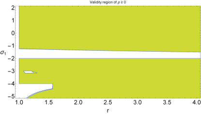
Figure 1: Validity of $\rho\geq 0$ given by (3.4) for the generic anisotropic fluid in Brans-Dicke theory when $\sigma_{2}=1$. The yellow regions represent the regions where $\gamma=1$ whereas the blue regions represent when $\gamma=-1$. Therefore, the green regions represent the regions where those two regions coincide. We have chosen the values $r_{0}=\phi_{0}=d=\omega_{0}=1$ and $\sigma_{2}=1$.

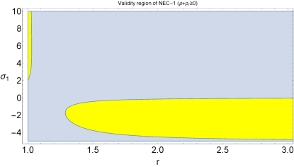
(a) NEC-1

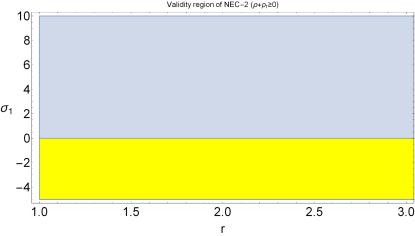
(b) NEC-2

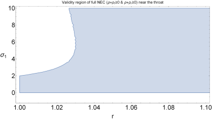
(c) NEC-near the throat

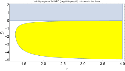
(d) NEC-not close to the throat

Figure 2: Validity of NEC-1 ($\rho+p_{r}\geq 0$) given by (3.5), NEC-2 ($\rho+p_{t}\geq 0$) given by (3.6) and the full condition for the validity of NEC ($\rho+p_{r}\geq 0$ and $\rho+p_{t}\geq 0$) for the generic anisotropic fluid in Brans-Dicke theory. The yellow regions represent the regions where $\gamma=1$ whereas the blue regions represent when $\gamma=-1$. For these plots, we have chosen the values $r_{0}=\phi_{0}=d=\omega_{0}=1$ and $\sigma_{2}=1$.

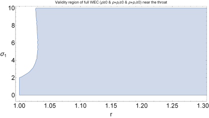
(a) WEC-near the throat

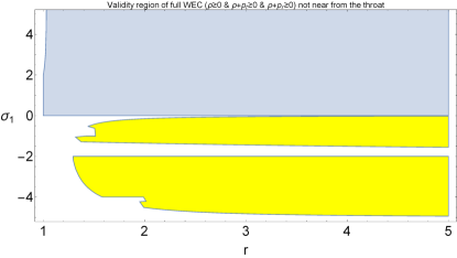
(b) WEC-not close to the throat

Figure 3: Validity of WEC ($\rho\geq 0$, $\rho+p_{r}\geq 0$ and $\rho+p_{t}\geq 0$) given by the validity of (3.4)-(3.6) for the generic anisotropic fluid in Brans-Dicke theory. The figure on the right represents the validity of WEC near the throat whereas the figure on the left shows the validity for locations that are not close to the throat. The yellow regions represent the regions where $\gamma=1$ whereas the blue regions represent when $\gamma=-1$. For these plots, we have chosen the values $r_{0}=\phi_{0}=d=\omega_{0}=1$ and $\sigma_{2}=1$.

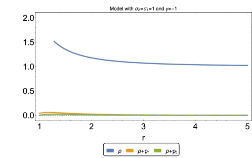
Figure 4: Energy density, sum of the radial pressure and the energy density and the sum of the lateral pressure and the energy density for the generic anisotropic fluid in Brans-Dicke theory where $\sigma_{1}=\sigma_{2}=1$ and $\gamma=-1$. We have further chosen the values $r_{0}=\phi_{0}=d=\omega_{0}=1$. For this model, the full WEC is always satisfied.

Let us now try to analyse the model for an arbitrary shape function parameter $\sigma_{2}$. In this case, we have three parameters, namely, $\gamma$ , $\sigma_{1}$ and $\sigma_{2}$. As we have said before, the sign of $\gamma$ is important but not its strength. Figs. 5 show region plots for the validity of the full NEC and WEC for positive and negatives values of $\gamma$. One can notice that it is not possible to model wormholes satisfying the full NEC everywhere for positive $\gamma$ since depending on the location of the observer, that energy condition would be valid or not. For negative values of $\gamma$, there are different models depending on $\sigma_{2}$ and $\sigma_{1}$ which ensures that the wormhole is supported by non-exotic matter at every point of the space. In those specific models, the full WEC is always satisfied.

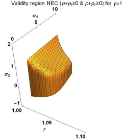
(a) NEC with $\gamma=1$

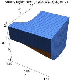
(b) NEC with $\gamma=-1$

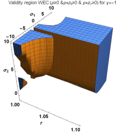
(c) WEC with $\gamma=-1$

Figure 5: Validity of NEC ($\rho+p_{r}\geq 0$ and $\rho+p_{t}\geq 0$) and WEC ($\rho\geq 0$, $\rho+p_{r}\geq 0$ and $\rho+p_{t}\geq 0$) given by the validity of (3.4)-(3.6) for the generic anisotropic fluid in Brans-Dicke theory. The figure on the left represents the validity of NEC for $\gamma=1$ whereas the figure on the centre represents the validity for $\gamma=-1$. Lastly, the figure on the right shows the validity of WEC for $\gamma=-1$. For these plots, we have chosen the values $r_{0}=\phi_{0}=d=\omega_{0}=1$.

3.2 Induced gravity

In this section, we will study the energy conditions for the Induced Gravity case. To recover this case, we must choose $n=2$ with $m>0$. Then, we have 4 free parameters, namely $m$, $\sigma_{1},\sigma_{2}$ and $\gamma$. Doing a similar approach as we did in the previous section, we can distinguish between models that do not violate the energy conditions. Without going into too much details as in the previous section, in this section we will only show the validity of the full NEC and full WEC. If WEC is valid, all the other energy conditions will be valid too. The validity of WEC will be true if all the following three inequalities hold,

$$\rho = -\frac{m\sigma_{1}^{3}r^{-(m+2)\sigma_{1}-1}}{(m+2)\sigma_{1}+1}+\frac{1}{16}\sigma_{1}^{2}r^{-(m+2)\sigma_{1}-2}\left(\frac{16m\sigma_{1}r^{-\sigma_{2}}}{(m+2)\sigma_{1}+\sigma_{2}+2}-\frac{16((m-2)\sigma_{1}+2)}{(m+2)\sigma_{1}+2}+\frac{1}{\pi}\right)$$ (3.7)

$$+\frac{\sigma_{1}^{2}(16\pi(m\sigma_{1}-\sigma_{2}+3)-(m+2)\sigma_{1}-\sigma_{2}-3)r^{-(m+2)\sigma_{1}-\sigma_{2}-3}}{16\pi((m+2)\sigma_{1}+\sigma_{2}+3)}$$

$$+\frac{\gamma\left(8\sigma_{1}^{3}+\sigma_{1}^{2}(6\sigma_{2}+26)+\sigma_{1}\left(\sigma_{2}^{2}+8\sigma_{2}+8\pi(\sigma_{2}-3)+21\right)-\sigma_{2}(\sigma_{2}+3)\right)r^{-2\sigma_{1}-\sigma_{2}-3}}{8\pi(2\sigma_{1}+\sigma_{2}+3)}$$

$$-\frac{\gamma\sigma_{1}(2\sigma_{1}+3)r^{-2\sigma_{1}-2}}{4\pi}+1\geq 0\,,$$

$$\rho+p_{r} = \frac{\gamma\left(4\sigma_{1}^{2}+\sigma_{1}(\sigma_{2}+11)-\sigma_{2}-1\right)r^{-2\sigma_{1}-\sigma_{2}-3}}{8\pi}-\frac{\gamma\sigma_{1}(2\sigma_{1}+5)r^{-2\sigma_{1}-2}}{4\pi}\geq 0\,,$$ (3.8)

$$\rho+p_{t} = \frac{\gamma(12\sigma_{1}-\sigma_{2}+1)r^{-2\sigma_{1}-\sigma_{2}-3}}{16\pi}-\frac{3\gamma\sigma_{1}r^{-2\sigma_{1}-2}}{4\pi}\geq 0\,.$$ (3.9)

Note that the validity of the last two inequalities do not depend on the parameter $m$. Hence, the validity of the full NEC will not depend on the parameter $m$. Figs. 6a and 6b show the validity of NEC for $\gamma=1$ and $\gamma=-1$ respectively. Exactly as the Brans-Dicke case, NEC cannot be true for every location when $\gamma$ is positive. Moreover, the problem comes near the throat. Hence, the full WEC will be also not true at every location for Induced Gravity when $\gamma$ is positive. On the other hand, for negative $\gamma$, it is possible to ensure the validity of NEC for some parameters $\sigma_{1}$ and $\sigma_{2}$. Fig. 6c shows the validity of WEC for $m=2$ and $\gamma=-1$. Since $\rho$ depends on $m$, the validity of WEC will depend on $m$ too. For bigger values of $m$, the validity of WEC is more constraint. However, it always exists a small range of values of $\sigma_{1}$ and $\sigma_{2}$ where WEC will be true at every location (even near the throat). From the figure one can notice that this small region is $-1\lesssim\sigma_{1}\lesssim 1$. Fig. 7 depicts the energy density and the sum of the pressures with the energy density for a model in this range, where $\sigma_{1}=0.5$. In the latter figure, we have further chosen $m=\sigma_{2}=2$ and $\gamma=-1$. One can see from the figure, that WEC is always true in this model.

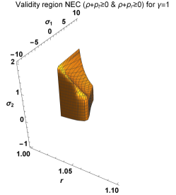
(a) NEC with $\gamma=1$

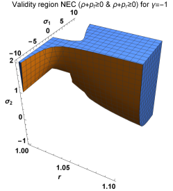
(b) NEC with $\gamma=-1$

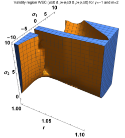
(c) WEC with $\gamma=-1$

Figure 6: Validity of NEC ($\rho+p_{r}\geq 0$ and $\rho+p_{t}\geq 0$) and WEC ($\rho\geq 0,$ $\rho+p_{r}\geq 0$ and $\rho+p_{t}\geq 0$) given by the validity of (3.7)-(3.9) for the generic anisotropic fluid in Induced Gravity. The figure on the left represents the validity of NEC for $\gamma=1$ whereas the figure on the centre represents the validity for $\gamma=-1$. Lastly, the figure on the right shows the validity of WEC for $\gamma=-1$ and $m=2$. For these plots, we have chosen the values $r_{0}=\phi_{0}=d=\omega_{0}=1$. We can notice that various model exist where the full WEC is valid for $\gamma=-1$ whereas for $\gamma=1$, it is not possible to find that NEC is valid for every location.

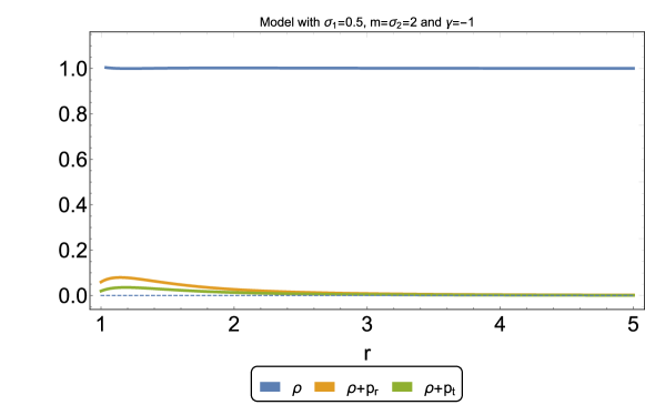
Figure 7: Energy density, sum of the radial pressure and the energy density and the sum of the lateral pressure and the energy density for the generic anisotropic fluid in Induced Gravity where $\sigma_{1}=0.5$, $\sigma_{2}=m=2$ and $\gamma=-1$. We have further chosen the values $r_{0}=\phi_{0}=d=\omega_{0}=1$. For this model, the full WEC is always satisfies.

4 Isotropic Fluid ($p_{r}=p_{t}=p$)

In this section, we will study the isotropic fluid case when $p_{r}=p_{t}=p$. By choosing this kind of fluid and substituting $e^{-b(r)}=1-\frac{\beta(r)}{r}$ in the field equations (2.20)-(2.22), we find the following differential equation for the shape function,

$$\frac{\gamma}{dr\kappa^{2}}{\phi_{0}}^{n}\left(\frac{d}{r}\right)^{n\sigma_{1}}\bigg{[}d^{2}r(n\sigma_{1}-1)\beta^{\prime}(r)+\left\{-2n{\sigma_{1}}^{3}(\sigma_{1}-1)+d^{2}\left(3-7n\sigma_{1}+2n{\sigma_{1}}^{2}-2n^{2}{\sigma_{1}}^{2}\right)\right\}\beta(r)$$

$$+2nr\sigma_{1}\left\{{\sigma_{1}}^{2}(\sigma_{1}-1)+d^{2}(3+n\sigma_{1}-\sigma_{1})\right\}\bigg{]}=0\,.$$ (4.1)

We can easily solve this equation analytically giving us the following shape function

$$\beta(r)=-\xi r+c_{1}r^{-\eta}\,,$$ (4.2)

where $c_{1}$ is an integration constant and for simplicity we have introduced the constants $A_{1}=d^{2}(n\sigma_{1}-1)$, $A_{2}=-2n{\sigma_{1}}^{3}(\sigma_{1}-1)+d^{2}\left\{3-7n\sigma_{1}+2n{\sigma_{1}}^{2}-2n^{2}{\sigma_{1}}^{2}\right\}$, $A_{3}=2n\sigma_{1}\left\{{\sigma_{1}}^{2}(\sigma_{1}-1)+d^{2}\left(3+n\sigma_{1}-\sigma_{1}\right)\right\}$, $\xi=\frac{A_{3}}{A_{1}+A_{2}}$ and $\eta=\frac{A_{2}}{A_{1}}$. At the throat $r=r_{0}$, we have the condition $\beta(r_{0})=r_{0}$. Using this relation, it is easily to get that the throat is located at $r_{0}=\left(\frac{c_{1}}{1+\xi}\right)^{\frac{1}{\eta+1}}$. Using the flaring-out condition at the throat, $\beta^{\prime}(r_{0})<1$, one notices that the condition $\eta>-1$ must be satisfied.

By replacing a power-law model described by (2.19) and the above form of the shape function into the modified Klein-Gordon equation (2.3), one can obtain the potential yielding

$$V(\phi) = \frac{2nc_{1}\eta\gamma\sigma_{1}{d}^{-\eta-3}{\phi_{0}}^{\frac{-\eta-3}{\sigma_{1}}}}{n\sigma_{1}+\eta+3}\phi^{\frac{n\sigma_{1}+\eta+3}{\sigma_{1}}}+\frac{\omega_{0}{\sigma_{1}}^{2}(1+\xi)(-2+2\sigma_{1}+m\sigma_{1})d^{-2}{\phi_{0}}^{-2/\sigma_{1}}}{m\sigma_{1}+2\sigma_{1}+2}{\phi}^{\frac{m\sigma_{1}+2\sigma_{1}+2}{\sigma_{1}}}$$

$$+ \frac{2n\gamma\xi\sigma_{1}d^{-2}{\phi_{0}}^{-2/\sigma_{1}}}{n\sigma_{1}+2}{\phi}^{\frac{n\sigma_{1}+2}{\sigma_{1}}}-\frac{\omega_{0}c_{1}{\sigma_{1}}^{2}(-1+\eta+2\sigma_{1}+m\sigma_{1})d^{-3-\eta}{\phi_{0}}^{\frac{-3-\eta}{\sigma_{1}}}}{m\sigma_{1}+2\sigma_{1}+\eta+3}\phi^{m+2+\frac{\eta+3}{\sigma_{1}}}+c_{0}\,,$$

where $c_{0}$ is an integration constant. In the latter, we will study the Brans-Dicke and Induced Gravity cases to analyse the regions when the energy conditions are valid.

4.0.1 Brans-Dicke theory

Taking $n=1$ and $m=-1$, we get $f(R,\phi)=\gamma R\phi$ which describes Brans-Dicke theory. We will discuss the behavior of $\beta(r)$, $\rho$ and $\rho+p$ by taking the special case where the parameters $d=\omega_{0}=c_{0}=\phi_{0}=1$, $\sigma_{1}=-2.4$, $r_{0}=1$ and $\gamma=-0.5$. The behavior of the shape function is shown in Fig. 9. This figure shows that $\beta(r)$ is increasing and also satisfy $\beta(r)<r$. The behavior of NEC and WEC are shown in Fig. 9. In that case, $\rho>0$ and $\rho+p>0$ are satisfied throughout the evolution. Then, all the energy conditions are satisfied for the parameter chosen. Thus, isotropic fluids satisfying the energy conditions can support wormholes in Brans-Dicke theory.

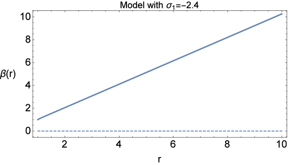
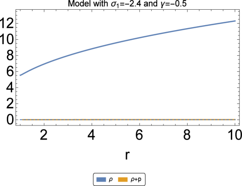
Figure 8: The behavior of $\beta(r)$ versus $r$ taking $n=1$, $m=-1$, $\sigma_{1}=-2.4$, $r_{0}=1$ in case of BD theory.

Figure 9: The behavior of $\rho$ and $\rho+p_{r}$ versus $r$ taking $n=1$, $m=-1$, $\sigma_{1}=-2.4$, $r_{0}=1$ for BD theory.

4.0.2 Induced gravity

Let us now explore Induced Gravity, where one needs to take $n=2$ and $m>0$. To analyse the properties of the wormhole in this theory, let us chose the parameters $\omega_{0}=-0.5$, $r_{0}=d=c_{0}=1$, $\phi_{0}=0.05$, $\sigma_{1}=-2.4$ and $\gamma=-0.5$. Fig. 11 shows the increasing behavior of shape function and validate the term $\beta(r)<r$. The behavior of NEC and WEC are shown in Fig. 11, which shows the validity of the energy conditions throughout the evolution. Then, exactly as in Brans-Dicke theory, in Induced gravity is possible to construct wormholes supported by an isotropic fluid satisfying the energy conditions.

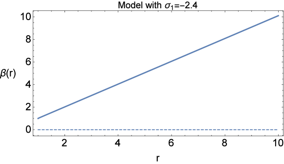
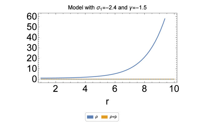
Figure 10: The behavior of $\beta(r)$ versus $r$ taking $n=2$, $m=2$, $\sigma_{1}=-2.4$, $r_{0}=1$ in the case of the Induced gravity.

Figure 11: Plot shows the evolution of $\rho$ and $\rho+p$ in case of Induced gravity for the parameters $n=2$, $m=2$, $\sigma_{1}=-2.4$, $r_{0}=1$, $\gamma=-0.5$.

5 Barotropic fluid with EoS $p_{r}=W(r)\rho$

In this section, we will choose a generic varying barotropic fluid with an EoS $p_{r}=W(r)\rho$ which involves radial pressure, energy density and a positive radial function $W(r)$. In 24a* , Rahaman et al. have used that type of EoS with a varying parameter. For this section, we will also assume a potential of the form

$$V(\phi)=\frac{V_{0}}{\phi^{\alpha}}\,.$$

Here $V_{0}$ is a constant. In the following, different forms of the function $W(r)$ will be adopted to analyse different barotropic fluids which can support wormholes.

5.1 $W(r)=W=Constant$

First we take $W(r)=W=constant$ which is a standard barotropic fluid. By replacing this form of EoS in the field equations (2.20)-(2.22), we obtain the following constraint,

$$\frac{1}{r\kappa^{2}}\left(\frac{d}{r}\right)^{-\alpha\sigma_{1}}{\phi_{0}}^{-\alpha}\bigg{[}-2\kappa^{2}r^{3}V_{0}(W+1)+2nr\gamma\sigma_{1}(-2+3W+n\sigma_{1}W){\phi_{0}}^{n+\alpha}\left(\frac{d}{r}\right)^{\sigma_{1}(n+\alpha)}$$

$$-r\omega_{0}{\sigma_{1}}^{2}(W+1){\phi_{0}}^{m+2+\alpha}\left(\frac{d}{r}\right)^{\sigma_{1}(m+2+\alpha)}+\omega_{0}{\sigma_{1}}^{2}(W+1){\phi_{0}}^{m+2+\alpha}\left(\frac{d}{r}\right)^{\sigma_{1}(m+2+\alpha)}\beta(r)$$

$$-\gamma{\phi_{0}}^{n+\alpha}\left(\frac{d}{r}\right)^{\sigma_{1}(n+\alpha)}\left\{(2-4n\sigma_{1}+7n\sigma_{1}W+2n^{2}{\sigma_{1}}^{2}W)\beta(r)+rW(2-n\sigma_{1})\beta^{\prime}(r)\right\}\bigg{]}=0\,.$$

The above equation cannot be easily solved analytically, so that we will explore some numerical interesting cases to study it.

5.1.1 Brans-Dicke theory

In case of Brans-Dicke we are using $n=1$, $m=-1$ and by varying the parameters $\omega_{0}$, $\sigma_{1}$, $\gamma$, $\alpha$, $W$, $\phi_{0}$, $V_{0}$ we will discuss the behavior of $\beta(r)$, $\beta^{\prime}(r)$, $\frac{\beta(r)}{r}$, $\beta(r)-r$, $\rho$, $\rho+p_{r}$ and $\rho+p_{t}$. In Fig. 12a, the behavior of the shape function is shown. This figure shows the increasing behavior and meet the inequality $\beta(r)<r$. It can be seen from Fig. 13a that $\beta(r)/r\rightarrow 0$ as $r\rightarrow\infty$ which means that the spacetime is asymptotically flat. Fig. 13b shows that $\beta(r)-r<0$, which fulfills the condition $1-\beta(r)/r>0$. The throat is then located at $r_{0}\approx 0.2114$ with $\beta(r_{0})=r_{0}$. The plot of $\beta^{\prime}(r)$ is shown in Fig. 12b and $\beta^{\prime}(r_{0})\approx-0.07093$ which fulfills the condition $\beta^{\prime}(r_{0})<1$. Evolution of the validity of NEC and WEC are shown in Fig. 14. Here $\rho>0$ and $\rho+p_{r}>0$ are satisfied throughout the evolution but $\rho+p_{t}>0$ is not satisfied. Then, the wormhole satisfy NEC-1 and WEC-1 but does not satisfy the full WEC.

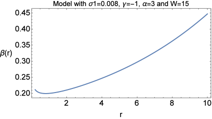
(a) Plot of $\beta(r)$

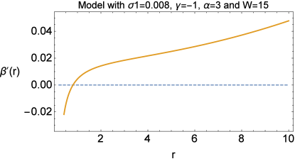
(b) Plot of $\beta^{\prime}(r)$

Figure 12: The behavior of $\beta(r)$ and $\beta^{\prime}(r)$ versus $r$ taking $\omega_{0}=-2$, $\sigma_{1}=0.008$, $\gamma=-1$, $\alpha=3$, $W=15$, $\phi_{0}=10$, $V_{0}=0.1$.

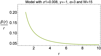
(a) Plot of $\frac{\beta(r)}{r}$

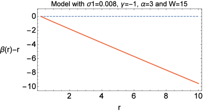
(b) Plot of $\beta(r)-r$

Figure 13: The behavior of $\frac{\beta(r)}{r}$ and $\beta(r)-r$ versus $r$ taking $\omega_{0}=-2$, $\sigma_{1}=0.008$, $\gamma=-1$, $\alpha=3$, $W=15$, $\phi_{0}=10$, $V_{0}=0.1$.

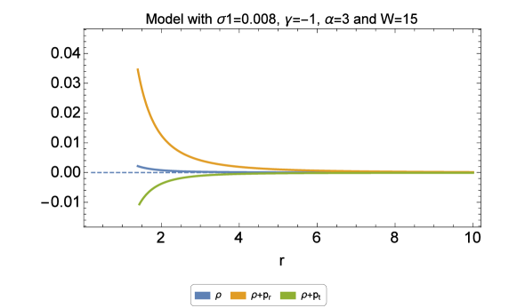
Figure 14: The behavior of $\rho$, $\rho+p_{r}$ and $\rho+p_{t}$ versus $r$ for the parameters $\omega_{0}=-2$, $\sigma_{1}=0.008$, $\gamma=-1$, $\alpha=3$, $W=15$, $\phi_{0}=10$, $V_{0}=0.1$.

5.1.2 Induced gravity

For Induced Gravity, we need to take $n=2$ and $m>0$ and then by varying the parameters $\omega_{0}$, $\sigma_{1}$, $\gamma$, $\alpha$, $W$, $\phi_{0}$, $V_{0}$, we will discuss the behavior of $\beta(r)$, $\beta^{\prime}(r)$, $\frac{\beta(r)}{r}$, $\beta(r)-r$, $\rho$, $\rho+p_{r}$ and $\rho+p_{t}$. In Fig. 15a, the behavior of the shape function $\beta(r)$ versus the radial coordinate is plotted. It can be seen that this function is increasing and then meet the inequality $\beta(r)<r$. From Fig. 16a, we can also notice that $\beta(r)/r\rightarrow 0$ as $r\rightarrow\infty$ which means that the spacetime is asymptotically flat. The plot in Fig. 16b shows that $\beta(r)-r<0$, which fulfills the condition $1-\beta(r)/r>0$. The throat is located at $r_{0}=0.2159$ with $\beta(r_{0})=r_{0}$. The plot of $\beta^{\prime}(r)$ is shown in Fig. 15b and $\beta^{\prime}(r_{0})=-0.108932$ which fulfills the flaring-out condition $\beta^{\prime}(r_{0})<1$. Evolution of NEC and WEC are then shown in Fig. 17. Here, exactly as in the Brans-Dicke case, $\rho>0$ and $\rho+p_{r}>0$ are satisfied throughout the evolution but $\rho+p_{t}>0$ is not satisfied in this case.

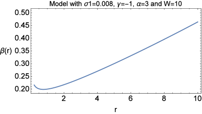
(a) Plot of $\beta(r)$

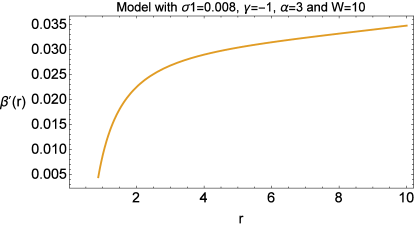
(b) Plot of $\beta^{\prime}(r)$

Figure 15: The behavior of $\beta(r)$ and $\beta^{\prime}(r)$ versus $r$ taking $\omega_{0}=-2$, $\sigma_{1}=0.008$, $\gamma=-1$, $\alpha=3$, $W=10$, $\phi_{0}=10$, $V_{0}=0.1$.

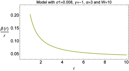
(a) Plot of $\frac{\beta(r)}{r}$

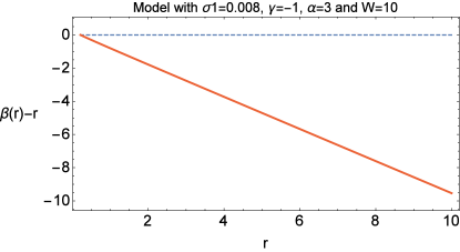
(b) Plot of $\beta(r)-r$

Figure 16: The behavior of $\frac{\beta(r)}{r}$ and $\beta(r)-r$ versus $r$ taking $\omega_{0}=-2$, $\sigma_{1}=0.008$, $\gamma=-1$, $\alpha=3$, $W=10$, $\phi_{0}=10$, $V_{0}=0.1$.

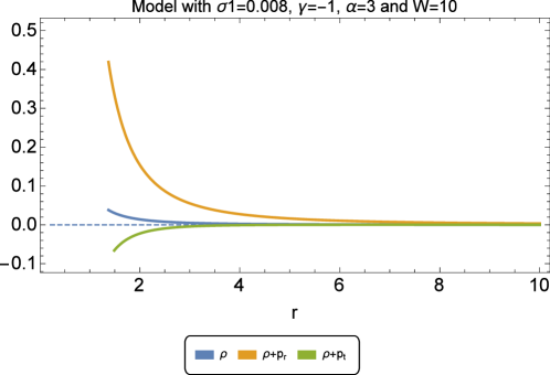
Figure 17: The behavior of $\rho$, $\rho+p_{r}$ and $\rho+p_{t}$ for the parameters $\omega_{0}=-2$, $\sigma_{1}=0.008$, $\gamma=-1$, $\alpha=3$, $W=10$, $\phi_{0}=10$, $V_{0}=0.1$.

5.2 $W(r)=Br^{l}$

Let us now explore the case where we take $W(r)=Br^{l}$ with $B$ and $l$ being positive constants. By using this EoS in the field equations (2.20)-(2.22), we get a constraint of the following form

$$\frac{1}{r\kappa^{2}}\left(\frac{d}{r}\right)^{-\alpha\sigma_{1}}{\phi_{0}}^{-\alpha}\bigg{[}-2\kappa^{2}r^{3}V_{0}(1+Br^{l})+2nr\gamma\sigma_{1}(-2+3Br^{l}+n\sigma_{1}Br^{l}){\phi_{0}}^{n+\alpha}\left(\frac{d}{r}\right)^{\sigma_{1}(n+\alpha)}$$

$$-r\omega_{0}{\sigma_{1}}^{2}(1+Br^{l}){\phi_{0}}^{m+2+\alpha}\left(\frac{d}{r}\right)^{\sigma_{1}(m+2+\alpha)}+\omega_{0}{\sigma_{1}}^{2}(1+Br^{l}){\phi_{0}}^{m+2+\alpha}\left(\frac{d}{r}\right)^{\sigma_{1}(m+2+\alpha)}\beta(r)$$

$$-\gamma{\phi_{0}}^{n+\alpha}\left(\frac{d}{r}\right)^{\sigma_{1}(n+\alpha)}\left\{(2-4n\sigma_{1}+7n\sigma_{1}Br^{l}+2n^{2}{\sigma_{1}}^{2}Br^{l})\beta(r)+rBr^{l}(2-n\sigma_{1})\beta^{\prime}(r)\right\}\bigg{]}=0\,.$$

Since this equation is very complicated to solve analytically, we will again solve this equation numerically for Brans-Dicke and Induced gravity cases. For Brans-Dicke theory we will choose the parameters $\omega_{0}=-2$, $\sigma_{1}=0.06$, $\gamma=-1$, $\alpha=5$, $B=2$, $l=5$ $\phi_{0}=10$, $V_{0}=0.1$. On the other hand, for Induced Gravity we set $n=2$, $m>0$, $\omega_{0}=-2$, $\sigma_{1}=0.008$, $\gamma=-1$, $\alpha=3$, $B=2$, $l=2.5$ $\phi_{0}=10$ and $V_{0}=0.1$. In Figs. 18a and 21a are depicted the shape function for the Brans-Dicke theory and Induced Gravity respectively. We can see that the shape functions satisfy the required condition $\beta(r)<r$ for both cases. The graphs in Figs. 19a and  22a show that $\beta(r)/r\rightarrow 0$ as $r\rightarrow\infty$, so that, again the metric is asymptotically flat in Brans-Dicke and Induced Gravity. Figs. 19b and 22b show that $\beta(r)-r<0$ for both theories, which fulfills the condition $1-\beta(r)/r>0$. The plot of $\beta^{\prime}(r)$ is shown in Fig. 18b and 21b for both theories where it can be notice that the flaring-out condition is also satisfied for both cases. Finally, Fig. 20 and 23 show the evolution of the validity of NEC and WEC for both theories. In these two theories we again have the same situation that $\rho>0$ and $\rho+p_{r}>0$ are satisfied throughout the evolution but $\rho+p_{t}>0$ is not satisfied.

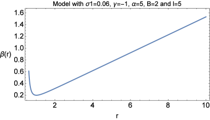
(a) Plot of $\beta(r)$

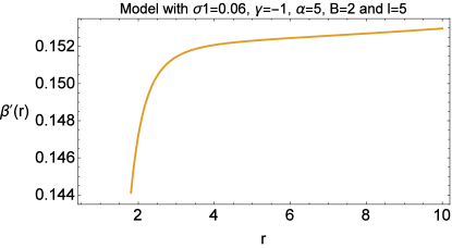
(b) Plot of $\beta^{\prime}(r)$

Figure 18: Plots of $\beta(r)$ and $\beta^{\prime}(r)$ versus $r$ for the Brans-Dicke theory taking $\omega_{0}=-2$, $\sigma_{1}=0.06$, $\gamma=-1$, $\alpha=5$, $B=2$, $l=5$ $\phi_{0}=10$, $V_{0}=0.1$. In this case we have that the throat is located at $r_{0}=0.61045$ and then $\beta^{\prime}(r_{0})=-6.11107$.

(a) Plot of $\frac{\beta(r)}{r}$

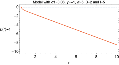
(b) Plot of $\beta(r)-r$

Figure 19: Plots of $\frac{\beta(r)}{r}$ and $\beta(r)-r$ versus $r$ for the Brans-Dicke theory for the parameters $\omega_{0}=-2$, $\sigma_{1}=0.06$, $\gamma=-1$, $\alpha=5$, $B=2$, $l=5$ $\phi_{0}=10$, $V_{0}=0.1$. In this case the throat is located at $r_{0}=0.61045$

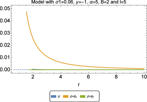
Figure 20: Plots of $\rho$, $\rho+p_{r}$ and $\rho+p_{t}$ versus $r$ for the Brans-Dicke theory for the parameters $\omega_{0}=-2$, $\sigma_{1}=0.008$, $\gamma=-1$, $\alpha=5$, $B=2$, $l=5$ $\phi_{0}=10$, $V_{0}=0.1$. In this case the throat is located at $r_{0}=0.61045$

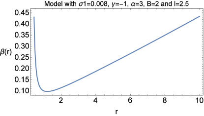
(a) Plot of $\beta(r)$

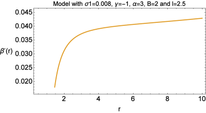
(b) Plot of $\beta^{\prime}(r)$

Figure 21: Plots of $\beta(r)$, $\beta^{\prime}(r)$ and $\frac{\beta(r)}{r}$ versus $r$ for Induced Gravity taking $\omega_{0}=-2$, $\sigma_{1}=0.008$, $\gamma=-1$, $\alpha=3$, $B=2$, $l=2.5$ $\phi_{0}=10$, $V_{0}=0.1$. Here we have that the throat is located at $r_{0}=0.43055$ and also $\beta^{\prime}(r_{0})=-4.15156$

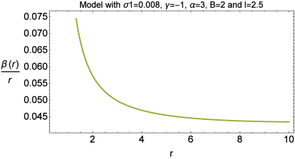
(a) Plot of $\frac{\beta(r)}{r}$

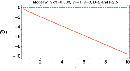
(b) Plot of $\beta(r)-r$

Figure 22: Plots of $\beta(r)$, $\beta^{\prime}(r)$ and $\frac{\beta(r)}{r}$ versus $r$ for induced gravity taking $\omega_{0}=-2$, $\sigma_{1}=0.008$, $\gamma=-1$, $\alpha=3$, $B=2$, $l=2.5$ $\phi_{0}=10$, $V_{0}=0.1$. Here we have that the throat is at $r_{0}=0.43055$

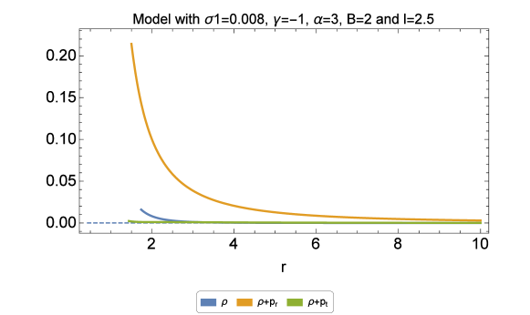
Figure 23: Plots show the evolution of $\rho$, $\rho+p_{r}$ and $\rho+p_{t}$ for for Induced Gravity for the parameters $\omega_{0}=-2$, $\sigma_{1}=0.008$, $\gamma=-1$, $\alpha=3$, $B=2$, $l=2.5$ $\phi_{0}=10$, $V_{0}=0.1$. Here we have that the throat is at $r_{0}=0.43055$

6 Summary and Conclusion

Wormhole solutions in GR do not satisfy all the standard energy conditions. Other approach is then to modify Einstein field equations in terms of an effective energy-momentum tensor that satisfy the energy bounds and the exotic part of the wormholes are supported by higher order curvature terms.

In this paper, we studied whether in $f(R,\phi)$ modified theory, the ordinary matter can support wormholes. In the last decades, it has been mentioned that in highly compacted astrophysical objects, pressures are anisotropic, which means that the tangential and radial pressures are not equal for such objects. Investigating the existence of wormholes for different kind of fluids are then an interesting question to address. To investigate this we have analyzed the behavior of NEC and WEC for three different supporting fluids: a barotropic fluid, an anisotropic fluid and an isotropic fluid. Additionally, we have constructed wormholes satisfying the flaring-out condition $\beta^{\prime}(r=r_{0})<1$ where $r_{0}$ is the throat which satisfies $\beta(r=r_{0})=r_{0}$.

To find analyse the physics of wormhole solutions, different methods have been discussed in the literature. One method is to find wormhole solutions giving a specific shape function. On the other hand, a second approach is considering the matter content and then calculate the shape function directly from the field equations.

In our manuscript, we have explored $f(R,\phi)$ gravity involving coupling between the Ricci scalar and matter field. Here the resulting equations are highly non-linear and complicated involving unknowns $p_{t}$, $p_{r}$, $\rho$, $a$, $b$, $f(R,\phi)$. Therefore, we have focused our study in a power-law case $f(R,\phi)=\gamma R\phi^{n}$, where $\gamma$ and $n$ are constants. Then, by choosing $n=1$ and $m=-1$, Brans-Dicke theory is recovered and by choosing $n=2$ and $m>0$, Induced Gravity is recovered. Then, for an anisotropic, isotropic and barotropic fluids, we have constructed wormhole solutions and then explore the energy conditions.

In the case of an anisotropic matter content, we assumed a specific form of the shape function (power-law type) to obtain a solution and then to check the existence of wormholes. Then, we investigated the validity of standard energy conditions. We have found that in both Brans-Dicke and induced gravity theories, an anisotropic generic fluid verifying all the energy conditions can support a wormhole geometry. However, to satisfy all the energy conditions, we must have negative values of $\gamma$. For positive values of $\gamma$, the matter given by the anisotropic fluid will violate some of the energy conditions.

In the case of an isotropic fluid $p_{r}=p_{t}=p$, it is possible to solve the field equations to get the shape function and the potential. The shape function then can be constraint to satisfy the wormhole’s conditions. This is valid for a generic power-law $f(R,\phi)$ gravity. Then, we found that isotropic fluids satisfying all the energy conditions (WEC and NEC) can support wormholes in both Brans-Dicke and induced gravity theories.

For an anisotropic matter satisfying a barotropic EoS $p_{r}=W(r)\rho$, the field equations are complicated to solve. Therefore, we studied some special cases numerically focusing on Brans-Dicke and induced gravity theories. This study was carried out by choosing some special values of the parameters. We analised the cases where the barotropic function is a constant $W(r)=W$ and also when $W(r)=Br^{l}$, where $B$ and $l$ are constants. For both cases, we have constraint the parameters in such a way that ensures the conditions to have a traversable wormhole geometry. In both cases, we have found some models where $\rho+p_{r}>0$ and also $\rho>0$ but $\rho+p_{t}$ can be negative, so that WEC is not always satisfy. Then, for our potential, barotropic fluids in Brans-Dicke and Induced Gravity do not satisfy all the energy conditions to support a wormhole geometry. Note that one can also assume a barotropic EoS $p_{t}=W(r)\rho$, when now the transverse pressure is related to the energy density. If ones carries out the same analysis mentioned above with the same potential, we also get a similar conclusion: wormholes can be constructed satisfying all the geometric required properties but the full WEC is not satisfy. For this case, one has that $\rho+p_{t}>0$ and also $\rho>0$ but $\rho+p_{r}$ can be negative.

References

• (1) P. Jordan (1955). Schwerkraft und Weltall (Friedrich Vieweg und Sohn, Braunschweig).
• (2) Faraoni, V.: Cosmology in Scalar-Tensor Gravity (Springer, 2004).
• (3) Brans, C. H. and Dicke, R. H.: Phys. Rev. 124 (1961) 925.
• (4) O. Bertolami and P.J. Martins, Phys. Rev. D 61, 064007 (2000); M.K. Mak and T. Harko, Europhys. Lett. 60, 155 (2002).
• (5) W. Chakraborty and U. Debnath, Int. J. Theor. Phys. 48, 232 (2009).
• (6) H. Motavali, S. Capozziello and M. Roshan, Phys. Lett. B 666 (2008) 10.
• (7) Y. Bisabr: Phys. Rev. D 86, 127503 (2012); M. Sharif and Saira Waheed, Int. J. Mod. Phys. D 21(2012) 1250082.
• (8) T Futamase and K Maeda, Phys Rev. D 39(1989)399, L Amendola, M Lttteno and F Occhlonero, lntem. J. Mod Phys A 5 (1990) 3861.
• (9) L. Amendola, Phys. Rev. D 60(1999)043501.
• (10) M Monkawa, Astrophys. J Left. 362 (1990) L37.
• (11) J. Yokohama, Phys. Lett. B 212 (1988) 273
• (12) O. Hrycyna and M. Szydlowski, JCAP 04(2009)026.
• (13) J. Bekenstem and M Mtlgrom, Astrophys. J. 286 (1984) 7.
• (14) C. Schimd et al., Phys. Rev. D 71, 083512 (2005).
• (15) Jai-chan Hwang and H. Noh, Phys. Rev. D 54(1996)1460-1473; Jai-chan Hwang, Class. Quantum Grav. 14 (1997) 1981 1991;S.Β Bahamonde, C.Β G.Β B hmer, F.Β S.Β N.Β Lobo and D.Β S ez-G mez, Universe 1 (2015) no.2, 186
• (16) F. Perrotta and C. Baccigalup, Phys. Rev. D 61(1996) 023507.
• (17) Pettorino, V. et al.: JCAP 01(2005)014.
• (18) Pace, F. et al.: MNRAS 437(2014)547 561.
• (19) Fan, Y., Wu, P. and Yu, H.: Phys. Lett. B 746 (2015) 230 236
• (20) Fan, Y., Wu, P. and Yu, H.: Phys. Rev. D 92(2015)083529.
• (21) Flamm, L.: Phys. Z. 17 (1916) 448.
• (22) Einstein, A. and Rosen, N.: Phys. Rev. 48 (1935) 73.
• (23) Wheeler, J. A.: Ann. Phys. (N.Y.) 2 (1957) 604.
• (24) Morris, M. S. and Thorne, K. S.: Am. J. Phys. 56 (1988)395; Morris, M. S., Thorne, K. S. and Yurtsever, U.: Phys. Rev. Lett. 61(1988)1446.
• (25) Edward Teo. Rotating traversable wormholes. Phys. Rev. D 58(1998)024014; Visser, M.: Phys. Rev. D 39(1989)3182-3184; Visser, M., Kar, S. and Dadhich, N.: Phys. Rev. Lett. 90(2003)201102; Bouhmadi-L pez, M., Lobo, F.S.N. and Mart n-Moruno, P.: J. Cosmol. Astropart. Phys. 11(2014)007.
• (26) F.S.N. Lobo, M.A. Oliveira, Phys. Rev. D 80(2009)104012; Bahamonde, S., Jamil, M., Pavlovic, P. and Sossich, M.: Phys. Rev. D 94(2016)044041.
• (27) Jamil, M., Momeni, D. and Myrzakulov, R.: Eur. Phys. J. C 73(2013)2267; Boehmer, C.G., Harko, T. and Lobo, F.S.N.: Phys. Rev. D 85 (2012) 044033.
• (28) Zubair, M., Waheed, S. and Ahmad, Y.: Eur. Phys. J. C 76 (2016) 444.
• (29) Agnese, A. G. and Camera, M. La.: Phys. Rev. D 51 (1995) 2011.
• (30) K. K. Nandi, A. Islam, and J. Evans, Phys. Rev. D 55 (1997)2497.
• (31) He, F. and Kim, S-W.: Phys. Rev. D 65(2002)084022.
• (32) E. Ebrahimi and N. Riazi.: Phys. Rev. D 81(2010)024036.
• (33) Capozziello, S. et al.: Phys. Rev. D 86(2012)127504.
• (34) Sebastian Bahamonde, Ugur Camci, Salvatore Capozziello and Mubasher Jamil, Phys. Rev. D 94(2016)084042.
• (35) Mohammad Reza Mehdizadeh, Mahdi Kord Zangeneh, and Francisco S.N. Lobo, Phys. Rev. D 91(2015)084004.
• (36) ACCETTA, F.S., CHODOS, A. and SHAO, B.: Nuclear Physics B333 (1990) 221-252.
• (37) Lambiase, G. et al.: JCAP. 07 (2015) 003.
• (38) Harko, T., Lobo, F. S. N., Mak, M.K. and Sushkov, S.V.: Phys. Rev. D 87 (2013) 067504.
• (39) Garcia, N.M. and Lobo, F.S.N.: Phys. Rev. D 82 (2010) 104018; Classical Quantum Gravity 28 (2011) 085018.
• (40) Lobo, F.S.N.: Phys. Rev. D 75 (2007) 064027.
• (41) Zubair, M. and Kousar, F.: EPJC. 76 (2016) 254.
• (42) Banerjee, N. and Pavon, D.: Phys. Lett. B 647 (2007) 477.
• (43) Tian, D. W.: arXiv:1508.02291.
• (44) Pavlovic, P. and Sossich, M.: Eur. Phys. J. C 75 (2015) 117.
• (45) Dent, J.B., Dutta, S. and Saridakis, E.N.: J. Cosmol. Astropart. Phys. 009 (2011) 1101.
• (46) Sotiriou, T.P., Li, B. and Barrow, J.D.: Phys. Rev. D 83 (2011) 104030.
• (47) Li, B., Sotiriou, T.P. and Barrow, J.D.: Phys. Rev. D 83 (2011) 104017.
• (48) Zhang, Y., et al.: J. Cosmol. Astropart. Phys. 015 (2011) 1107.
• (49) Bhattacharya, S. and Chakraborty, S.: arXiv:1506.03968v2.
• (50) Rahaman, F. et al., Acta Phys. Polon. B, 40 (2009) 25.