Lifshitz transition and thermoelectric properties of bilayer graphene

Abstract

This is a numerical study of thermoelectric properties of ballistic bilayer graphene in the presence of trigonal warping term in the effective Hamiltonian. We find, in the mesoscopic samples of the length $L>10\,\mu{}$m at sub–Kelvin temperatures, that both the Seebeck coefficient and the Lorentz number show anomalies (the additional maximum and minimum, respectively) when the electrochemical potential is close to the Lifshitz energy, which can be attributed to the presence of the van Hove singularity in a bulk density of states. At higher temperatures the anomalies vanish, but measurable quantities characterizing remaining maximum of the Seebeck coefficient still unveil the presence of massless Dirac fermions and make it possible to determine the trigonal warping strength. Behavior of the thermoelectric figure of merit ($ZT$) is also discussed.

I Introduction

It is known that thermoelectric phenomena provide a valuable insight into the details of electronic structure of graphene and other relativistic condensed-matter systems that cannot be solely determined by conductance measurements Dol15 . Such a fundamental perspective has inspired numerous studies on Seebeck and Nernst effects in mono- (MLG) and bilayer (BLG) graphenes Zue09 ; Wei09 ; Che09 ; Hwa09 ; Nam10 ; Wan10 ; Wan11 ; Wys13 as well as in other two-dimensional systems New94 ; Cao15 ; Sex16 ; Sev17 . The exceptionally high thermal conductivity of graphenes has also drawn a significant attention Pet11 ; Bal11 ; YXu14 ; Zha15 ; Cro16 ; Zha16 after a seminal work by Balandin et al. Bal08 . A separate issue concerns thermal and thermoelectric properties of tailor-made graphene systems Dol15 ; Che10 ; Hua11 ; Lia12 ; Sev13 ; Hos15 ; Ann17 , including superlattices Che10 , nanoribbons Hua11 ; Lia12 ; Sev13 ; Hos15 , or defected graphenes Hos15 ; Ann17 , for which peculiar electronic structures may result in high thermoelectric figures of merit $ZT>2$ at room temperature Sev13 ; Hos15 .

Unlike in conventional metals or semiconductors, thermoelectric power in graphenes can change a sign upon varying the gate bias Zue09 ; Wei09 ; Che09 , making it possible to design thermoelectronic devices that have no analogues in other materials Che15 . In BLG the additional bandgap tunability Mac06b ; Min07 ; Zha09 was utilized to noticeably enhance the thermoelectric power in a dual-gated setup Wan11 .

At sufficiently low temperatures, one can expect thermolectric properties of BLG to reflect most peculiar features of its electronic structure. These features include the presence (in the gapless case) of three additional Dirac points in the vicinity of each of primary Dirac points $K$ and $K^{\prime}$ Mac06a ; Orl12 ; Kat12 ; Mac13 . In turn, when varying chemical potential the system is expected to undergo the Lifshitz transition at $\mu=\pm{}E_{L}$ (the Lifshitz energy) Mac13 . What is more, electronic density of states (DOS) shows van Hove singularities at $\mu=\pm{}E_{L}$. Unlike in systems with Mexican-hat band dispersion, for which diverging DOS appears at the bottom of the conduction band and at the top of the valence band Sex16 ; Sev17 , in BLG each van Hove singularity separates populations of massless Dirac-Weyl quasiparticles ($|\mu|<E_{L}$) with approximately conical dispersion relation, and massive chiral quasiparticles ($|\mu|>E_{L}$) characterized by the effective mass $m_{\rm eff}\approx{}0.033\,m_{e}$, with $m_{e}$ being the free-electron mass. Although the value of $E_{L}$ is related to several directly-measurable quantities, such as the minimal conductivity Mog09 ; Rut14b ; Rut16 , available experimental results cover the full range of $E_{L}\sim{}0.1\!-\!1\,$meV Mac13 .

The purpose of this work is to show that thermoelectric measurements in ballistic BLG (see Fig. 1) can provide new insights into the nature of quasiparticles near the charge-neutrality point and allow one to estimate the Lifshitz energy. We consider a relatively large, rectangular sample of ballistic BLG (with the length $L=17.7\,\mu$m, and the width $W=20\,L$), and calculate its basic thermoelectric properties (including the Seebeck coefficient $S$ and the Lorentz number ${\cal L}$) within the Landauer-Büttiker formalism Pau03 ; Esf06 . Our main findings are outlined in Fig. 1, where $N_{\rm max}^{S}$ ($N_{\rm min}^{\cal L}$) – the number of maxima (minima) of $S$ (${\cal L}$) appearing for $\mu>0$ is indicated in the $E_{L}\,$–$\,T$ parameter plane. For instance, a handbook value of $E_{L}/k_{B}\approx{}10\,$K Dre81 leads to the anomalies, including additional extrema at $\mu\approx{}E_{L}$, at sub–Kelvin temperatures. We further show that even for $T\gtrsim{}1\,$K (at which $N_{\rm max}^{S}=N_{\rm min}^{\cal L}=1$) the value of $E_{L}$ determines the carrier concentration corresponding to the remaining maximum of $S$ (or the minimum of ${\cal L}$).

The paper is organized as follows: The model and theory are described in Sec. II, followed by the numerical results and discussions on the conductance, thermopower, validity of the Wiedemann-Franz law, the role of phononic thermal conductivity, and the figure of merit (Sec. III). A comparison with the linear model for transmission-energy dependence (see Appendix A) is also included. The conclusions are given in Sec. IV.

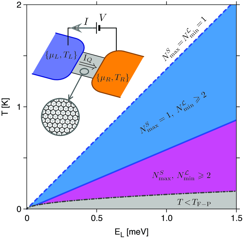
Figure 1: The system studied numerically in the paper (inset) and the thermoelectric phase diagram (main) for Bernal-stacked bilayer graphene. Thermal and electric currents ($I_{Q},I$) flow between the leads, modeled as infinitely-doped graphene regions with electrochemical potentials $\mu_{L(R)}\rightarrow\infty$ (at a fixed $\mu_{R}\!-\!\mu_{L}\equiv{}eV$, with the electron charge $-e$ and the voltage $V$), and temperatures $T_{L(R)}$, attached to the rectangular sample. Additional gate electrodes (not shown) are used to tune the chemical potential in the sample area $\mu$ at zero bias between the layers. The number of distinct maxima of the Seebeck coefficient ($N_{\rm max}^{S}$) and minima of the Lorentz factor ($N_{\rm min}^{\cal L}$), occurring for $0\!<\!\mu\!<\!\infty$, are indicated in the Lifshitz energy – temperature parameter plane. The border of the Fabry-Pérot transport regime $T\!<\!T_{\rm F-P}$ (in which $N_{\rm max}^{S},N_{\rm min}^{\cal L}\gg{}1$), corresponding to the system length $L=10^{4}\,l_{\perp}=17.7\,\mu$m, is also depicted.

II Model and Theory

II.1 The Hamiltonian

We start our analysis from the four-band effective Hamiltonian for low-energy excitations Mac13 , which can be written as

$$H=\xi\left(\begin{array}[]{cccc}0&v_{F}{}\pi&\xi\,t_{\perp}&0\\ v_{F}{}\pi^{\dagger}&0&0&v_{3}{}\pi\\ \xi\,t_{\perp}&0&0&v_{F}{}\pi^{\dagger}\\ 0&v_{3}{}\pi^{\dagger}&v_{F}{}\pi&0\end{array}\right),$$ (1)

where the valley index $\xi=1$ ($-1$) for $K$ ($K^{\prime}$) valley, $v_{F}=\sqrt{3}\,t_{0}a/(2\hbar)\simeq{}10^{6}\,$m/s is the asymptotic Fermi velocity defined via the intralayer hopping $t_{0}=3.16\,$eV and the lattice parameter $a=0.246\,$nm, $\pi=\hbar{}e^{-i\theta}(-i\partial_{x}+\partial_{y})$, $\theta$ denotes the angle between the main system axis and the armchair direction. (For the numerical calculations, we set $\hbar{}v_{F}=0.673\,$eV$\cdot$nm.) The nearest-neighbor interlayer hopping is $t_{\perp}=0.381\,$eV Kuz09 defining $l_{\perp}{}=\hbar{}v_{F}/t_{\perp}=1.77\,$nm, and $v_{3}=v_{F}{}t^{\prime}/t_{0}$ with $t^{\prime}$ being the next-nearest neighbor (or skew) interlayer hopping.

The Hamiltonian (1) leads to the bulk dispersion relation for electrons Mac06a ; Mac13

$$E_{\pm}^{(e)}(\mbox{\boldmath$k$}) =\left[\frac{1}{2}t_{\perp}^{2}+\left(v_{F}^{2}+\frac{1}{2}v_{3}^{2}\right)k^{2}\pm\sqrt{\Gamma(\mbox{\boldmath$k$})}\right]^{1/2},$$

$$\Gamma(\mbox{\boldmath$k$}) =\frac{1}{4}\left(t_{\perp}^{2}\!-\!\hbar^{2}v_{3}^{2}k^{2}\right)^{2}+\hbar^{2}v_{F}^{2}k^{2}\left(t_{\perp}^{2}\!+\!\hbar^{2}v_{3}^{2}k^{2}\right)$$ (2)

$$+2\xi{}\,t_{\perp}{}\hbar^{3}v_{3}v_{F}^{2}k^{3}\cos{}3\varphi,$$

where $\mbox{\boldmath$k$}\equiv{}(k_{x},k_{y})$ is the in-plane wavevector (with $\mbox{\boldmath$k$}=0$ referring to K or K’ point), $k=|\mbox{\boldmath$k$}|$, and the angle $0\leqslant\varphi<2\pi$ can be defined as the argument $\mbox{arg}\,z$ of a complex number

$$z=e^{-i\theta}(k_{x}+ik_{y}).$$ (3)

For holes, we have $E_{\pm}^{(h)}(\mbox{\boldmath$k$})=-E_{\pm}^{(e)}(\mbox{\boldmath$k$})$ elhofoo .

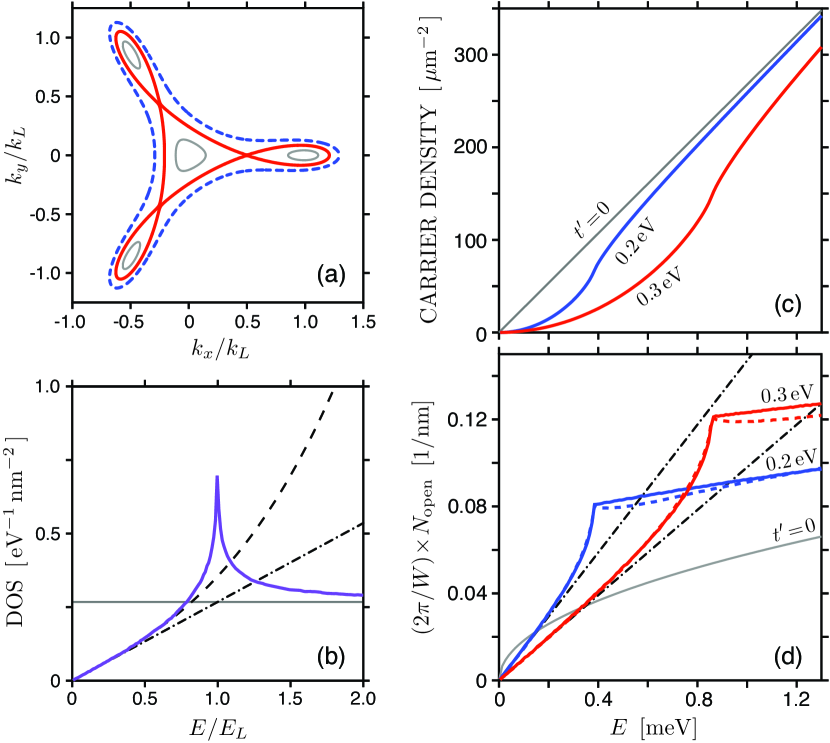
Figure 2: Physical consequences of the dispersion relation given by Eq. (2). (a) Equienergy surfaces for $E=0.5\,E_{L}$ (grey solid lines), $E=E_{L}$ (red solid line), and $E=1.5\,E_{L}$ (blue dashed line) for the crystallographic orientation $\theta=0$. (b) Density of states (purple solid line) and the approximating expressions given by Eqs. (7), (8), and (9) (grey solid, black dashed, and black dotted-dashed line, respectively). (c) Carrier density and (d) the number of open channels for different values of $t^{\prime}$ (specified for each line). Solid and dashed lines in panel (d) corresponds to $\theta=0$ and $\theta=\pi/6$, dotted-dashed lines represent the approximating Eq. (12).

II.2 Low-energy electronic structure

Basic consequences of Eq. (2) are illustrated in Fig. 2. In the energy range $|E|<E_{L}$, with the Lifshitz energy

$$E_{L}=\frac{1}{4}t_{\perp}\left(\frac{v_{3}}{v_{F}}\right)^{2},$$ (4)

there are four distinct parts of the Fermi surface (see Fig. 2a), centered at $z=z_{0},\dots,z_{3}$, where $z_{0}=0$, $z_{j}=k_{L}\exp(2\pi{}ij/3),j=1,2,3$, and

$$k_{L}=\frac{t_{\perp}{}v_{3}}{\hbar{}v_{F}^{2}}.$$ (5)

For $|E|\geqslant{}E_{L}$ the Fermi surface becomes connected, and the transition at $E=\pm{}E_{L}$ is accompanied by the van Hove singularity in the density of states $\rho(E)$ (see Fig. 2b), which can be defined (for electrons) via

$$\int_{0}^{E}dE^{\prime}\rho({E^{\prime}})\equiv n(E)=\frac{{\cal A}(E)}{\pi^{2}},$$ (6)

where $n(E)$ is the physical carrier density (taking into account spin and valley degeneracies $g_{s}=g_{v}=2$) depicted in Fig. 2c, and ${\cal A}(E)$ denotes the area bounded by the Fermi surface in the $(k_{x},k_{y})$ plane mcycfoo . In particular, taking the limit of $t^{\prime}\rightarrow{}0$ we have

$$\rho_{\,t^{\prime}\rightarrow{}0}(|E|\ll{}t_{\perp})\approx\frac{2m_{\rm eff}}{\pi{}\hbar^{2}}=\frac{t_{\perp}}{\pi{}(\hbar{}v_{F})^{2}}\equiv{}\rho_{0},$$ (7)

where we have introduced the effective mass relevant in the absence of trigonal warping ($E_{L}=0$). At finite $t^{\prime}$ ($E_{L}>0$) the value of $\rho_{0}$ defined in Eq. (7) is approached by the actual $\rho(E)$ for $|E|\gtrsim{}E_{L}$ (see Fig. 2b). Also, in the $t^{\prime}\neq{}0$ case, we find that the approximating formula

$$\rho(E)\approx\frac{\rho_{0}|E|}{E_{L}}\left[1+0.33\left({E}/{E_{L}}\right)^{2}\right],$$ (8)

reproduces the actual $\rho(E)$ with $1\%$ accuracy for $|E|\leqslant{}E_{L}/2$ (being the energy interval most relevant for discussion presented in the remaining parts of this paper). For $|E|\ll{}E_{L}$, leaving only the leading term on the right-hand side of Eq. (8) brought us to

$$\rho(|E|\ll{}E_{L})\approx\frac{4|E|}{\pi(\hbar{}v_{3})^{2}},$$ (9)

which can be interpreted as a double-monolayer DOS with the Fermi velocity replaced by $v_{3}$.

Although the trigonal-warping effects become hardly visible in $\rho(E)$ for $E\gtrsim{}E_{L}$, characteristic deformations of the Fermi surface can be noticed also for $E\gg{}E_{L}$. We point out that a compact quantity taking this fact into account, which can be determined directly from Eq. (2) without resorting to quantum transport simulations, is the number of propagating modes (open channels) $N_{\rm open}(\theta,E)$ presented in Fig. 2d. It can be defined as a total number of solutions, with real $k_{x}$, of equations

$$E^{(p)}_{+}(k_{x},q\Delta{}k_{y})=E,\ \ \ \ \ E^{(p)}_{-}(k_{x},q\Delta{}k_{y})=E,$$ (10)

where $p=e$ for electrons ($E>0$) or $p=h$ for holes ($E<0$), $q=0,\pm{}1,\pm{}2,\dots$, and $\Delta{}k_{y}=2\pi/W$ (we suppose the periodic boundary conditions along the $y$-axis), that correspond to a chosen sign the group velocity, e.g. $\left(v_{g}\right)^{(p)}_{\pm,q}=\partial{}E^{(p)}_{\pm}(k_{x},q\Delta{}k_{y})/\partial{k_{y}}>0$. Apart from the $t^{\prime}\rightarrow{}0$ limit, for which

$$N_{\rm open}(t^{\prime}\rightarrow{}0,|E|\ll{}t_{\perp})\approx 2\,\sqrt{\frac{{|E|t_{\perp}}}{(\hbar{}v_{F})^{2}}}\,\frac{1}{\Delta{}k_{y}},$$ (11)

the number of open channels is anisotropic and shows the periodicity with a period $\pi/3$. In the low-energy limit

$$N_{\rm open}(\,\theta,|E|\ll{}E_{L}\,)\approx 2F(\theta)\,\frac{|E|}{\hbar{}v_{3}}\,\frac{1}{\Delta{}k_{y}},$$ (12)

where

$$F(\theta) =1+\sum_{j=1,2,3}\left[1-\frac{8}{9}\cos^{2}\left(\theta+\frac{2\pi}{3}j\right)\right]^{1/2},$$ (13)

$$\approx 3.126+0.029\,\cos{}6\theta.$$

The anisotropy is even more apparent for $|E|\gtrsim{}E_{L}$. In particular, $N_{\rm open}(\theta=0,E)$ grows monotonically with increasing $E$, whereas $N_{\rm open}(\theta=\pi/6,E)$ has a shallow minimum at $E\approx{}1.11{}E_{L}$.

It is also visible in Fig. 2d that the effects of increasing $t^{\prime}$ are essentially opposite at different energy ranges: For $|E|\gtrsim{}E_{L}$, $N_{\rm open}$ grows systematically with $t^{\prime}$; for $|E|\ll{}E_{L}$ we have $N_{\rm open}\propto{}1/t^{\prime}$ following from Eq. (12). Such a feature has no analogues in behaviors of other characteristics presented in Fig. 2.

II.3 Thermoelectric properties

In the linear-response regime, thermoelectric properties of a generic nanosystem in graphene are determined via Landauer-Büttiker expressions for the electrical and thermal currents Lan57 ; But85

$$I =-\frac{g_{s}g_{v}e}{h}\int{}dE\,T(E)\left[f_{L}(E)\!-\!f_{R}(E)\right],$$ (14)

$$I_{Q} =\frac{g_{s}g_{v}}{h}\int{}dE\,T(E)\left[f_{L}(E)\!-\!f_{R}(E)\right](E\!-\!\mu),$$ (15)

where $g_{s}=g_{v}=2$ are spin and valley degeneracies, $T(E)\equiv{}\mbox{Tr}({\bf t}{\bf t}^{\dagger})$ with ${\bf t}$ being the transmission matrix Rut14b , $f_{L(R)}$ is the distribution functions for the left (right) lead with electrochemical potential $\mu_{L(R)}$ and temperature $T_{L(R)}$. Assuming that $\mu_{L}-\mu_{R}\equiv{}-eV$ and $T_{L}-T_{R}\equiv{}\Delta{}T$ are infinitesimally small [hereinafter, we refer to the averages $\mu=(\mu_{L}+\mu_{R})/2$ and $T=(T_{L}+T_{R})/2\,$], we obtain the conductance $G$, the Seebeck coefficient $S$, and the electronic part of the thermal conductance $K_{\rm el}$, as follows Esf06

$$G =\left.\frac{I}{V}\right|_{\Delta{}T=0}=e^{2}L_{0},$$ (16)

$$S =-\left.\frac{V}{\Delta{}T}\right|_{I=0}=\frac{L_{1}}{eTL_{0}},$$ (17)

$$K_{\rm el} =\left.\frac{I_{Q}}{\Delta{}T}\right|_{I=0}=\frac{L_{0}L_{2}-L_{1}^{2}}{TL_{0}},$$ (18)

where $L_{n}$ (with $n=0,1,2$) is given by

$$L_{n}=\frac{g_{s}g_{v}}{h}\int{}dE\,T(E)\left(-\frac{\partial{}f_{\rm FD}}{\partial{}E}\right)(E-\mu)^{n},$$ (19)

with $f_{\rm FD}(\mu,T,E)=1/\left[\,\exp\left((E\!-\!\mu)/k_{B}T\right)+1\,\right]$ the Fermi-Dirac distribution function.

By definition, the Lorentz number accounts only the electronic part of the thermal conductance,

$${\cal L}=\frac{K_{\rm el}}{TG}=\frac{L_{0}L_{2}-L_{1}^{2}}{e^{2}T^{2}L_{0}^{2}}.$$ (20)

The thermoelectric figure of merit accounts the total thermal conductance ($K_{\rm tot}=K_{\rm el}+K_{\rm ph}$)

$$ZT=\frac{TGS^{2}}{K_{\rm tot}}=\left(\frac{K_{\rm el}}{K_{\rm el}+K_{\rm ph}}\right)\frac{L_{1}^{2}}{L_{0}L_{2}-L_{1}^{2}},$$ (21)

where the phononic part can be calculated using

$$K_{\rm ph}=\frac{1}{2\pi}\int{}d\omega\,\hbar{}\omega\frac{\partial{}f_{\rm BE}}{\partial{}T}{\cal T}_{\rm ph}(\omega),$$ (22)

with $f_{\rm BE}(T,\omega)=1/\left[\,\exp\left(\hbar\omega/k_{B}{}T\right)-1\,\right]$ the Bose-Einstein distribution function and ${\cal T}_{\rm ph}(\omega)$ the phononic transmission spectrum. For BLG in a gapless case considered in this work, we typically have $K_{\rm ph}\sim{}K_{\rm el}$ (see Sec. IIID) phonofoo . As ${\cal T}_{\rm ph}(\omega)$ in Eq. (22) is generally much less sensitive to external electrostatic fields than $T(E)$ in Eq. (18) it should be possible — at least in principle — to independently determine $K_{\rm ph}$ and $K_{\rm el}$ in the experiment.

It can be noticed that ultraclean ballistic graphene shows approximately linear transmission to Fermi-energy dependence $T(E)\propto{}|E|$ (where $E=0$ corresponds to the charge-neutrality point) Two06 ; Dan08 ; Kum16 ; limofoo . Straightforward analysis (see Appendix A) leads to extremal values of the Seebeck coefficient as a function of the chemical potential

$$S_{\rm max}=-S_{\rm min}\approx{}k_{B}/e=86\,\mu\text{V/K},$$ (23)

providing yet another example of a material characteristic given solely by fundamental constants Two06 ; Nai08 . Similarly, the Lorentz number reaches, at $\mu=0$, the maximal value given by

$${\cal L}_{\rm max}=\frac{9\,\zeta(3)}{2\ln{}2}\left(\frac{k_{B}}{e}\right)^{2}=2.37\,{\cal L}_{\rm WF},$$ (24)

with ${\cal L}_{\rm WF}=\frac{1}{3}\pi^{2}(k_{B}/e)^{2}$ being the familiar Wiedemann-Franz constant. Although the disorder and electron-phonon coupling may affect the above-mentioned values, existing experimental works report $S_{\rm max}$ and ${\cal L}_{\rm max}$ close to the given by Eqs. (23) and (24) for both MLG and BLG, provided the temperature is not too low Zue09 ; Wei09 ; Che09 ; Hwa09 ; Nam10 ; Wan10 ; Cro16 .

At low temperatures, the linear model no longer applies, partly due to the contribution from evanescent modes Two06 ; Sny07 , and partly due to direct trigonal-warping effects on the electronic structure (see subsection IIB). For this reason, thermoelectric properties calculated numerically from Eqs. (16)–(21) are discussed next.

III Results and discussion

III.1 Zero-temperature conductivity

For $T\rightarrow{}0$ Eq. (16) leads to the conductivity

$$\sigma(T\!\rightarrow{}\!0)=\frac{G(T\!\rightarrow{}\!0)L}{W}=\frac{g_{0}L}{W}\,\mbox{Tr}({\bf t}{\bf t}^{\dagger}),$$ (25)

with the conductance quantum $g_{0}=4e^{2}/h$. As the right-hand side of Eq. (25) is equal to $\mbox{Tr}({\bf t}{\bf t}^{\dagger})$ with a constant prefactor, $\sigma(T\!\rightarrow{}\!0)$ gives a direct insight into the transmission-energy dependence that defines all the thermoelectric properties [see Eqs. (16)–(21)].

In order to determine the transmission matrix ${\bf t}$ for a given electrochemical potential $\mu$ we employ the computational scheme similar to the presented in Ref. Rut14b . However, at finite-precision arithmetics, the mode-matching equations become ill-defined for sufficiently large $L$ and $\mu$, as they contain both exponentially growing and exponentially decaying coefficients. This difficulty can be overcome by dividing the sample area into $N_{\rm div}$ consecutive, equally-long parts, and matching wave functions for all $N_{\rm div}\!+\!1$ interfaces ndivfoo .

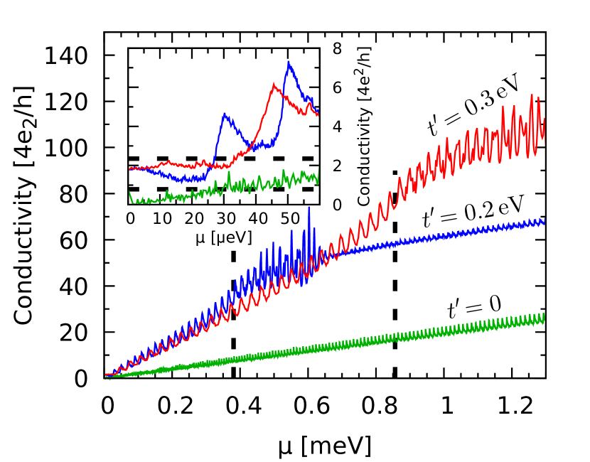
Figure 3: Zero-temperature conductivity [see Eq. (25) in the main text] for $L=W/20=10^{4}\,l_{\perp}=17.7\,\mu$m and $\theta=0$ theta0foo plotted as a function of the chemical potential. The value of skew-interlayer hopping $t^{\prime}$ is specified for each line. Remaining tight-binding parameters are given below Eq. (1) in the main text. Vertical lines mark values of the Lifshitz energy, given by Eq. (4), for $t^{\prime}=0.2\,$eV and $t^{\prime}=0.3\,$eV. Inset is a zoom in, for low chemical potentials, with horizontal lines depicting $\sigma=2\,\sigma_{\rm MLG}=(8/\pi)\,e^{2}/h$ and $\sigma=6\,\sigma_{\rm MLG}$.

Numerical results are presented in Fig. 3. A striking feature of all datasets is the presence of quasiperiodic oscillations of the Fabry-Pérot type. Although such oscillations can be regarded as artifacts originating from a perfect, rectangular shape of the sample area (vanishing immediately when e.g. samples with nonparallel edges are considered, see Ref. Rut14c ) their periodic features are useful to benchmark the numerical procedure applied.

In particular, for $t^{\prime}=0$, the conductivity shows abrupt features at energies associated with resonances at normal incidence ($k_{y}=0$) Sny07 , namely

$$E_{n}(t^{\prime}=0)\approx{}\pm{}\hbar{}v_{F}{}l_{\perp}\left(\frac{\pi{}n}{L}\right)^{2},\ \ \ \ n=1,2,3,\dots,$$ (26)

where the approximation refers to the parabolic dispersion relation applying for $|E_{n}|\ll{}t_{\perp}$, or equivalently for $n\ll{}L/(\pi{}l_{\perp})\approx{}3180$ in our numerical example. In turn, the separation between consecutive resonances is

$$\Delta{}E_{n}(t^{\prime}=0) =|E_{n+1}\!-\!E_{n}|\approx{}\frac{2n\!+\!1}{t_{\perp}}\left(\frac{\pi{}\hbar{}v_{F}}{L}\right)^{2}$$

$$\approx 2\,\frac{\pi{}\hbar{}v_{F}}{L}\sqrt{\frac{|E_{n}|}{t_{\perp}}},$$ (27)

with the last approximation corresponding to $n\gg{}1$.

For $t^{\prime}\neq{}0$ the analysis is much more cumbersome even at low energies, as we have resonances associated with four distinct Dirac cones. However, resonances at normal incidence associated with the central cone, occurring at $E_{n}\approx{}\pi\hbar{}v_{3}n/L$ ($n=\pm{}1,\pm{}2,\dots$), allow us to estimate the order of magnitude of the relevant separation as

$$\Delta{}E_{n}(t^{\prime}\neq{}0) \sim\frac{\pi\hbar{}v_{3}}{L}=2\,\frac{\pi{}\hbar{}v_{F}}{L}\sqrt{\frac{E_{L}}{t_{\perp}}}\equiv{}k_{B}T_{\rm F-P},$$ (28)

finding that the period of Fabry-Pérot oscillations is now energy-independent and should be comparable with $\Delta{}E_{n}(0)$ given by Eq. (27) for $\mu=E_{n}\approx{}E_{L}(t^{\prime})$. The data displayed in Fig. 3 show that the oscillation period is actually energy-independent in surprisingly-wide interval of $\mu\lesssim{}1.5E_{L}$, with the multiplicative factor $\left.\Delta{}E_{n}(t^{\prime})/\Delta{}E_{n}(0)\right|_{\mu=E_{L}(t^{\prime})}\approx{}3$. The oscillation amplitude is also enhanced, in comparison to the $t^{\prime}=0$ case, for $\mu\lesssim{}1.5E_{L}$. For $\mu\gtrsim{}1.5E_{L}$, both the oscillation period and amplitude are noticeably reduced, resembling the oscillation pattern observed for the $t^{\prime}=0$ case. It is also visible in Fig. 3, that the mean conductivity (averaged over the oscillation period) linearly increase with $\mu$ for $\mu\lesssim{}E_{L}$, with a slope weakly dependent on $t^{\prime}$. Such a behavior indicates that $\mbox{Tr}({\bf t}{\bf t}^{\dagger})<N_{\rm open}$ [see Fig. 2(d)] what can be interpreted as a backscattering (or transmission reduction) appearing when different classes of quasiparticles are present in the leads and in the sample area. For larger $\mu$, the transmission reduction is still significant, but its dependence on $t^{\prime}$ is weaken, and the sequence of lines from Fig. 2(d) is reproduced.

Detailed explanation of the above-reported observations, in terms of simplified models relevant for $|\mu|\ll{}E_{L}$ and for $|\mu|\gtrsim{}E_{L}$, will be presented elsewhere. Here we only notice that the linear model for transmission-energy dependence is justified, for $|\mu|\lesssim{}E_{L}$, with the numerical results presented in Fig. 3.

The rightmost equality in Eq. (28) defines the Fabry-Pérot temperature, which can be written as

$$T_{\rm F-P}=\frac{\pi{}\,t_{\perp}{}t^{\prime}l_{\perp}}{k_{B}{}t_{0}{}L}=13890\,\text{K}\times{}\frac{t^{\prime}\,l_{\perp}}{t_{0}L}.$$ (29)

For $L=10^{4}{}\,l_{\perp}$, we obtain $T_{\rm F-P}=88\,$mK if $t^{\prime}=0.2\,$eV, or $T_{\rm F-P}=132\,$mK if $t^{\prime}=0.3\,$eV. For higher temperatures, Fabry-Pérot oscillations are smeared out due to thermal excitations involving transmission processes from a wider energy window [see Eqs. (16) and (19)].

III.2 Thermopower and Wiedemann-Franz law

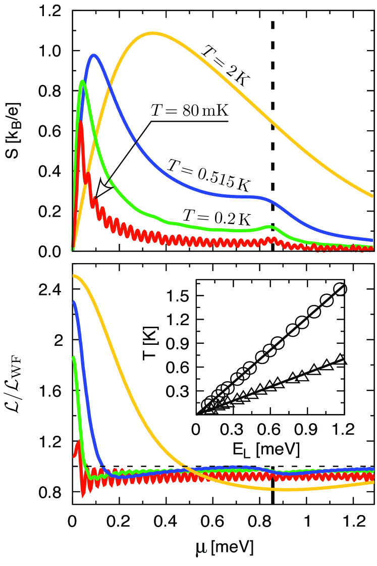
Figure 4: Seebeck coefficients $S$ and Lorentz number ${\cal L}$ for $t^{\prime}=0.3\,$eV, as a function of the chemical potential. The temperature is specified for each line in top panel and is the same in both panels. Vertical lines mark the Lifshitz energy; horizontal line in bottom panel corresponds to the Wiedemann-Franz value ${\cal L}={\cal L}_{\rm WF}=\frac{1}{3}\pi^{2}(k_{B}/e)^{2}$. Inset shows crossover temperatures, corresponding to vanishing of the secondary maximum of $S$ (triangles) and minimum of ${\cal L}$ (circles), plotted as functions of the Lifshitz energy, together with the best-fitted linear functions [see Eqs. (30) and (31)].

As the finite-$T$ conductivity is simply given by a convolution of $T(E)=\mbox{Tr}({\bf t}{\bf t}^{\dagger})$ with the derivative of the Fermi-Dirac function, we proceed directly to the numerical analysis of the Seebeck coefficient and the Lorentz number given by Eqs. (17)–(20) mottfoo . In Fig. 4, these thermoelectric properties are displayed as functions of $\mu$, for a fixed $t^{\prime}=0.3\,$eV (corresponding to $E_{L}/k_{B}\approx{}10\,$K) and varying temperature. Quasiperiodic oscillations are still prominent in datasets for the lowest presented temperature, $T=80\,\text{mK}\approx{}0.6\,T_{\rm F-P}$, although it is rather close to $T_{\rm F-P}$. This is because all the abrupt features of $T(E)$ are magnified when calculating $S$, or ${\cal L}$, since they affect the nominator and the denominator in the corresponding Eq. (17), or Eq. (20), in a different manner. For $T=0.2\,\text{K}\approx{}1.5\,T_{\rm F-P}$ the oscillations vanish for $S$ and are strongly suppressed for ${\cal L}$; instead, we observe the anomalies: the secondary maximum of $S$ and minimum of ${\cal L}$, located near $\mu=E_{L}$. The secondary maximum of $S$ vanishes for $T=T_{\star}^{S}=0.515\,$K, but ${\cal L}$ still shows the two shallow minima at this temperature. (We find that the minima of ${\cal L}$ merge at $T_{\star}^{\cal L}=1.20\,\text{K}=2.33\,T_{\star}^{S}$, the corresponding dataset is omitted for clarity.) For $T=2\,K$, each of $S$ and ${\cal L}$ shows a single extremum for $\mu>0$.

The crossover temperatures $T_{\star}^{S}$ and $T_{\star}^{\cal L}$ as functions of $E_{L}$, varied in the range corresponding to $0.1\,\text{eV}\leqslant{}t^{\prime}\leqslant{}0.35\,\text{eV}$, are also plotted in Fig. 4 (see the inset). The least-squares fitted lines are given by

$$T_{\star,{\rm fit}}^{S}=0.0504(5)\times E_{L}/k_{B},$$ (30)

$$T_{\star,{\rm fit}}^{\cal L}=0.1176(3)\times E_{L}/k_{B},$$ (31)

with standard deviations of the last digit specified by numbers in parentheses.

These findings can be rationalized by referring to the onset on low-energy characteristics given in Sec. IIB (see Fig. 2). In particular, the abrupt features of $T(E)$ near $E=E_{L}$, attributed to the van Hove singularity of $\rho(E)$ shown in Fig. 2(b), or to the anisotropy of $N_{\rm open}(\theta,E)$ in Fig. 2(d), are smeared out when calculating thermoelectric properties for energies of thermal excitations

$$k_{B}T\gtrsim{}0.1\,E_{L}.$$ (32)

However, some other features, related to trigonal-warping effects on $N_{\rm open}(\theta,E)$ or $n(E)$ [see Fig. 2(c)] away from $E=E_{L}$, visible in thermoelectric properties, may even be observable at higher temperatures.

III.3 Comparison with the linear model for transmission-energy dependence

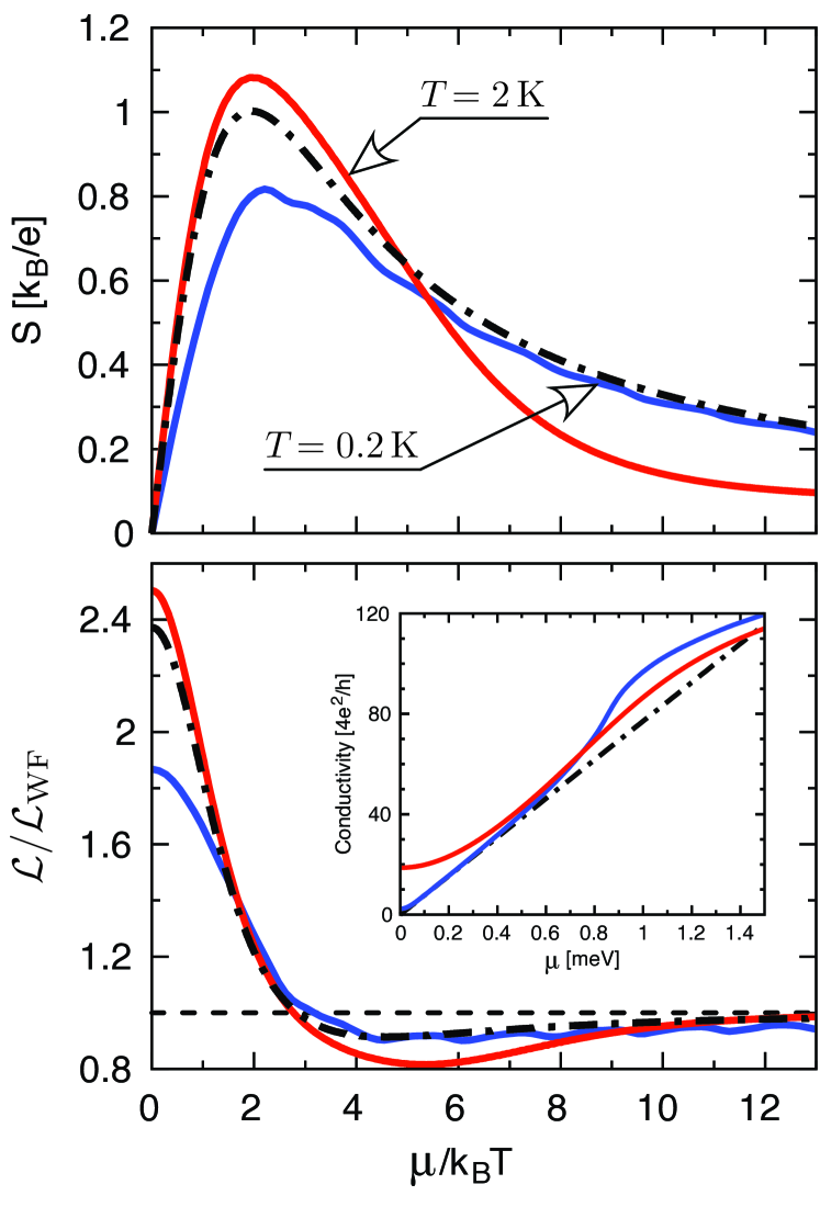
Figure 5: Same as Fig. 4 but plotted versus the dimensionless variable $\mu/(k_{B}T)$. Solid lines in both panels represent the datasets for $T=0.2\,$K and $T=2\,$K. Dashed-dotted lines correspond to Eqs. (43) and (44) in Appendix A, following from the linear model for transmission-energy dependence. Dashed line in bottom panel marks ${\cal L}={\cal L}_{\rm WF}$. Inset shows the finite-$T$ conductivity (solid lines) $\sigma=GL/W$ [see Eqs. (16) and (19) in the main text] and the linear fit (dash-dot line) to the corresponding $T=0$ dataset in Fig. 3.

In Fig. 5 we display the selected numerical data from Fig. 4, for $T=0.2\,$K and $T=2\,$K, as functions of $\mu/(k_{B}T)$ [solid lines] in order to compare them with predictions of the linear model for transmission-energy dependence $T(E)\propto{}|E|$ [dashed-dotted lines] elaborated in Appendix A. For $T=2\,$K, both $S$ and ${\cal L}$ show an agreement better than $10\%$ with the linear model for $\mu\lesssim{}E_{L}\approx{}5\,k_{B}T$. For $T=0.2\,$K, larger deviations appear for low chemical potentials due to the influence of transport via evanescent waves, which are significant for $\mu<\hbar{}v_{F}/L\approx{}2-3\,k_{B}T$. For larger $\mu$, a few-percent agreement with the linear model is restored, and sustained as long as $\mu\lesssim{}E_{L}\approx{}40\,k_{B}T$.

Another remarkable feature of the results presented in Fig. 5 becomes apparent when determining the extrema: The maximal thermopower corresponds to $\mu_{\rm max}^{(S)}/(k_{B}T)=2.0$ at $T=2\,$K, or to $\mu_{\rm max}^{(S)}/(k_{B}T)=2.2$ at $T=0.2\,$K; the minimal Lorentz number corresponds to $\mu_{\rm min}^{({\cal L})}/(k_{B}T)=5.4$ at $T=2\,$K, or to $\mu_{\rm min}^{({\cal L})}/(k_{B}T)=4.6$ at $T=0.2\,$K. In other words, an almost perfect agreement with the linear model [see, respectively, the second equality in Eq. (45), or the second equality in Eq. (46) in Appendix A] is observed provided that

$$\frac{\hbar{}v_{F}}{L}\ \ll{}\ k_{B}T\sim\mu_{\rm max}^{(S)}\sim\mu_{\rm min}^{({\cal L})}\ \ll{}\ E_{L}.$$ (33)

In consequence, the effects that we describe may be observable for the sample length $L>10\,\mu$m.

III.4 Electronic and phononic parts of the thermal conductance

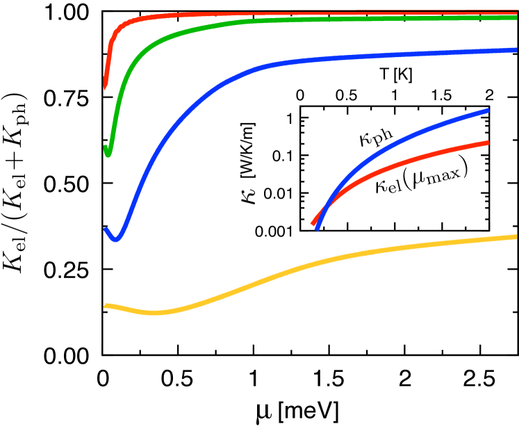
Figure 6: Relative electronic contribution to the thermal conductance for $t^{\prime}=0.3\,$eV as a function of the chemical potential. The temperatures are (top to bottom) $T=80\,$mK, $0.2\,$K, $0.515\,$K, and $2\,$K. Inset shows phononic [blue line] and electronic [red line] thermal conductivities ($\kappa=KL/(2dW)$, with $d=0.335\,$mn the separation between layers) as functions of temperature, with the chemical potential fixed at $\mu=\mu_{\rm max}$ corresponding to the maximal Seebeck coefficient.

Before discussing the thermoelectric figure of merit $ZT$ we first display, in Fig. 6, values of the dimensionless prefactor in the last expression of Eq. (21), quantifying relative electronic contribution to the thermal conductance. The phononic transmission spectrum [see Eq. (22)] was calculated numerically by employing, for the sample length $L=17.7\,\mu$m, the procedure presented by Alofi and Srivastava Alo13 adapting the Callaway theory Cal59 for mono-nand few-layer graphenes kaphfoo . The results show that in sub-Kelvin temperatures the electronic contribution usually prevails, even if the system is quite close to the charge-neutrality point, as one can expect for a gapless conductor. For $T>1\,$K, however, the phononic contribution overrules the electronic one in the full range of chemical potential considered.

A direct comparison of the phononic and the electronic and thermal conductivities calculated in the physical units (see inset in Fig. 6) further shows that, if the chemical potential is adjusted to $\mu_{\rm max}\equiv{}\mu_{\rm max}^{(S)}$ for a given temperature, both properties are of the same order of magnitude up to $T=2\,$K. Also, for $\mu=\mu_{\rm max}$, we find that $K_{\rm el}=K_{\rm ph}$ at the temperature $T_{\rm el-ph}\approx{}0.3\,$K, which is almost insensitive to the value of $t^{\prime}$.

III.5 Maximal performance versus temperature

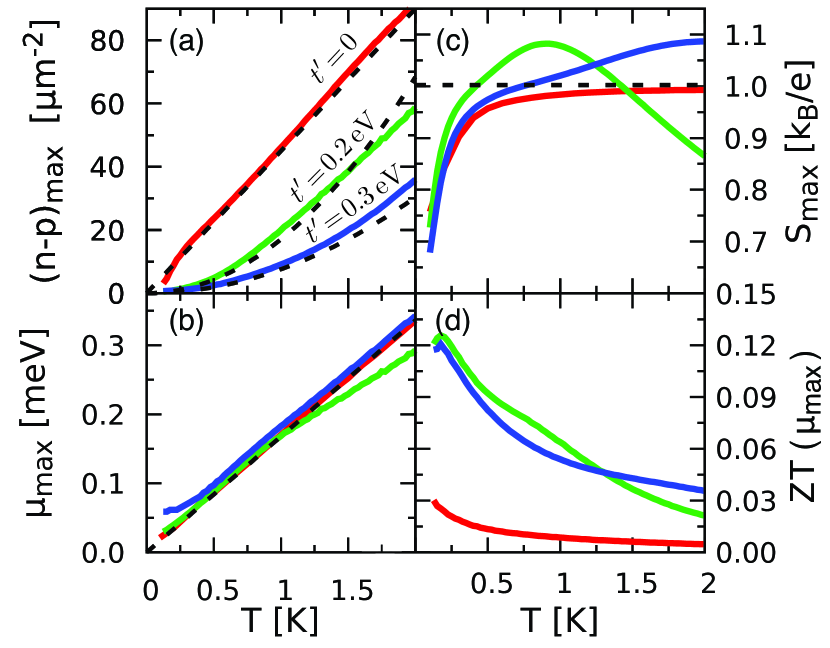
Figure 7: Effective carrier concentration $(n\!-\!p)_{\rm max}$ (a) and chemical potential $\mu_{\rm max}$ (b) corresponding to the maximal Seebeck coefficient $S_{\rm max}$ (c) as functions of temperature. The figure of merit $ZT(\mu_{\rm max})$ (d) is also displayed. Solid lines represent the numerical results for different values of $t^{\prime}$ [ specified in panel (a) ]. Dashed lines mark predictions of the linear model for transmission-energy dependence $T(E)\propto{}|E|$.

In Fig. 7 we present parameters characterizing the maximal thermoelectric performance for a given temperature ($0<T\leqslant{}2\,$K). As the existing experimental works refer to the carrier concentration rather then to the corresponding chemical potential, we focus now on the functional dependence of the former on $T$ (and $t^{\prime}$).

Taking into account that the maximal performance is expected for $\mu\sim{}k_{B}T$ (see previous subsection), and that a gapless system is under consideration, one cannot simply neglect the influence of minority carriers. For the conduction band ($\mu>0$), the effective carrier concentration can be written as

$$n\!-\!p =\int_{0}^{\infty}dE\,\rho(E)f(\mu,E)$$

$$-\int_{-\infty}^{0}dE\,\rho(E)[1-f(\mu,E)],$$ (34)

where we have supposed the particle-hole symmetry $\rho(E)=\rho(-E)$. [For the valence band ($\mu<0$), the effective concentration $p\!-\!n$ is simply given by the formula on the right-hand side of Eq. (34) with an opposite sign.] Next, the approximating Eqs. (7) and (8) for the density of states lead to

$$n\!-\!p \approx\rho_{0}{}k_{B}T$$

$$\times\begin{cases}{\displaystyle\,y,}&\ \text{if }\ t^{\prime}=0,\\ &\vspace{-1em}\textstyle\\ {\displaystyle\,\tau_{L}\left[\,{\cal I}_{1}(y)+0.33\,\tau_{L}^{2}\,{\cal I}_{3}(y)\,\right],}&\ \text{if }\ t^{\prime}\neq 0,\end{cases}$$ (35)

where $y=\mu/k_{B}T$, $\tau_{L}=k_{B}T/E_{L}$, and we have defined

$${\cal I}_{n}(y)=\int_{-y}^{\infty}{}\frac{(x+y)^{n}}{e^{x}+1}dx-\int_{y}^{\infty}{}\frac{(x-y)^{n}}{e^{x}+1}dx.$$ (36)

(In particular, ${\cal I}_{0}(y)=y$.) Numerical evaluation of the integrals in Eq. (35) for $y=y_{\rm max}$ given by Eq. (45) in Appendix A brought us to

$$(n\!-\!p)_{\rm max} \approx\rho_{0}{}k_{B}T$$

$$\times\begin{cases}{\displaystyle 1.949}&\text{if }\ t^{\prime}=0,\\ &\vspace{-1em}\textstyle\\ {\displaystyle 3.269\,\tau_{L}\!\left(1\!+\!3.23\,\tau_{L}^{2}\right)}&\text{if }\ t^{\prime}\neq 0.\end{cases}$$ (37)

In turn, the carrier concentration corresponding to the maximum of $S$ for a given $T$ is determined by the value of $E_{L}$. [A similar expression for the minimum of ${\cal L}$, see Eq. (46) in Appendix A, is omitted here.]

Solid lines in Fig. 7(a) show the values of $(n\!-\!p)_{\rm max}$ calculated from Eq. (34) for the actual density of states and the chemical potential $\mu=\mu_{\rm max}$ [displayed with solid lines in Fig. 7(b)] adjusted such that the Seebeck coefficient, obtained numerically from Eq. (17), reaches the conditional maximum ($S_{\rm max}$) [see Fig. 7(c)] at a given temperature $T$ (and one of the selected values of $t^{\prime}=0$, $0.2\,$eV, or $0.3\,$eV). The numerical results are compared with the linear-model predictions (dashed lines in all panels), given explicitly by Eq. (37) [Fig. 7(a)] or Eq. (45) in Appendix A [Figs. 7(b) and 7(c)]. Again, the linear model shows a relatively good agreement with corresponding data obtained via the mode-matching method; moderate deviations are visible for $t^{\prime}\neq{}0$ when $\mu_{\rm max}\gtrsim{}E_{L}/2$. In such a range, both $\rho(E)$ no longer follows the approximating Eq. (9), and the sudden rise of $T(E)$ near $E\approx{}E_{L}$ starts to affect thermoelectric properties.

Fig. 7(c) and Fig. 7(d) display, respectively, the maximal Seebeck coefficient ($S_{\rm max}$) and figure of merit ($ZT(\mu_{\rm max})$) as functions of temperature. For $t^{\prime}\neq{}0$, the former shows broad peaks, centered near temperatures corresponding to $\mu_{\rm max}\approx{}0.4\,E_{L}$, for which the prediction of the linear model [see Eq. (45) in Appendix A] is slightly exceeded (by less then $10\%$), whereas for $t^{\prime}=0$ a monotonic tempereture dependence, approaching the linear-model value, is observed. The figure of merit (calculated for $\mu=\mu_{\rm max}$) shows relatively fast temperature decay due to the role of phononic thermal conductivity (see Sec. IIID). We find that $ZT(\mu_{\rm max})$, although being relatively small, is noticeably elevated in the presence of trigonal warping in comparison to the $t^{\prime}=0$ case.

The behavior of $S_{\rm max}$ presented in Fig. 7(c) suggests a procedure, allowing one to determine the trigonal-warping strength via directly measurable quantities.

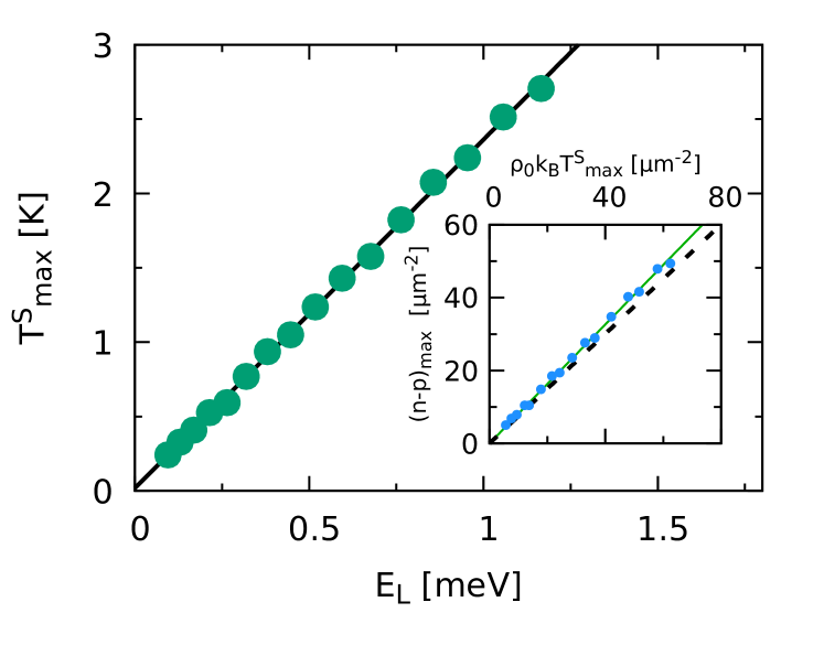
Figure 8: Temperature corresponding to the maximal thermopower as a function of the Lifshitz energy (datapoints). Least-squares fitted linear dependence [see Eq. (38)] is also displayed (line). Inset shows the carrier concentration versus $\rho_{0}k_{B}T_{\rm max}^{S}$, together with the model prediction (dashed line) and the linear fit (solid line) [see Eqs. (37) and (39)].

For any $t^{\prime}\neq{}0$, one can determine a unique global maximum of $S=S(\mu,T)$, which is reached at $\mu=\mu_{\rm max}^{S}$ and $T=T_{\rm max}^{S}$. Our numerical findings for $0.1\,\text{eV}\leqslant{}t^{\prime}\leqslant{}0.35\,\text{eV}$ are presented in Fig. 8, where we have plotted (instead of $\mu_{\rm max}^{S}$), the optimal effective concentration $(n\!-\!p)_{\rm max}^{S}$ [see the inset]. The best-fitted lines displayed Fig. 8 are given by

$$T_{{\rm max},\,{\rm fit}}^{S} =0.203(2)\times E_{L}/k_{B},$$ (38)

$$\left(n-p\right)_{{\rm max},\,{\rm fit}}^{S} =0.816(5)\times\rho_{0}{k_{B}}T_{\rm max}^{S},$$ (39)

where numbers in parentheses are standard deviations for the last digit. A few-percent deviation of the actual $(n\!-\!p)_{{\rm max}}^{S}$ from predictions of the linear model [see dashed line in the inset, obtained from Eq. (37) by setting $\tau_{L}=k_{B}T_{{\rm max},\,{\rm fit}}^{S}/E_{L}\approx{}0.20\,$] is relatively small taking into account that the existence of a global maximum of $S(\mu,T)$ is directly link to the breakdown of the linear model occurring for $\mu\sim{}k_{B}T\gtrsim{}E_{L}$ (and therefore is not observed in the $t^{\prime}=0$ case).

We further notice that Eqs. (38) and (39) provide direct relations between the two independent driving parameters corresponding to the optimal thermopower, $T_{{\rm max}}^{S}$ and $(n\!-\!p)_{{\rm max}}^{S}$, and the trigonal warping strength quantified by $E_{L}$.

IV Conclusions

We have investigated the thermopower, violation of the Wiedemann-Franz law, and the thermoelectric figure of merit, for large ballistic samples of bilayer graphene in the absence of electrostatic bias between the layers (a gapless case) and close to the charge-neutrality point. Although the thermoelectric performance is not high in such a parameter range, we find that low-temperature behavior of thermoelectric properties is determined by microscopic parameters of the tight-binding Hamiltonian, including the skew-interlayer hopping integral responsible for the trigonal warping, and by the relativistic nature of effective quasiparticles (manifesting itself in linear energy dependence of both the density of states and the electrical conductivity).

In particular, at sub-Kelvin temperatures, clear signatures of the Lifshitz transition, having forms of anomalies in chemical-potential dependences of the Seebeck coefficient and the Lorentz number, occurs in a vicinity of the Lifshitz energy (defined by the microscopic parameters and quantifying the trigonal-warping strength). The anomalies are blurred out by thermal excitations above the crossover temperatures (different for the two thermoelectric properties) that are directly proportional to the Lifshitz energy.

At higher temperatures (of the order of $1\,$K) the trigonal-warping strength can be determined from thermoelectric measurements following one of the two different approaches: (i) finding the carrier concentration corresponding to the maximal thermopower as a function of temperature, or (ii) finding the optimal temperature, i.e., such that thermopower reaches its global maximum. The first possibility is linked to the properties of massless quasiparticles, due to which the carrier concentration corresponding to the maximal thermopower depends approximately quadratically on temperature and reciprocally on the Lifshitz energy. On the other hand, existence of unique optimal temperature (equal to $2\,K$ if the handbook value of the Lifshitz energy $E_{L}/k_{B}\approx{}10\,$K is supposed) is related the gradual conductivity enhancement, and subsequent suppression of the thermopower, with increasing population of thermally-excited massive quasiparticles above the Lifshitz energy.

To conclude, we have show that thermoelectric measurements may complement the list of techniques allowing one to determine tight-binding parameters of bilayer-graphene Hamiltonian. Unlike the well-established techniques Mac13 (or the other recently-proposed Rut14b ; Rut16 ), they neither require high-magnetic field measurements nor refer to conductivity scaling with the system size. Instead, the proposed single-device thermoelectric measurements must be performed on large ballistic samples (with the length exceeding $10\,\mu$m), such that quantum-size effects define the energy scale much smaller then the Lifshitz energy.

As we have focused on clean ballistic systems, several factors which may modify thermoelectric properties of graphene-based devices, including the disorder Mac13 , lattice defects Dre10 , or magnetic impurities Uch11 , are beyond the scope of this study. However, recent progress in quantum-transport experiments on ultraclean free-standing monolayer samples exceeding $1\,\mu$m size Kum16 ; Ric15 allows us to expect that similar measurements would become possible in bilayer graphene soon. Also, as the effects we describe are predicted to appear away from the charge-neutrality point, the role of above-mentioned factors should be less significant than for phenomena appearing precisely at the charge-neutrality point, such as the minimal conductivity May11 ; Sam16 . Similar reasoning may apply to the role of interaction-induced spontaneous energy gap Rtt11 ; Fre12 ; Bao12 (we notice that experimental values coincide with energy scales defined by quantum-size effects, e.g., $\hbar{}v_{F}/L\approx{}3\,$meV for $L=250\,$nm in Ref. Bao12 ).

Note added in proof. Recently, we become aware of theoretical works on strained monolayer graphene reporting quite similar, double-peak spectra of the Seebeck coefficient for sufficiently high uniaxial strains Man17 .

Appendix A Linear model for transmission-energy dependence

At sufficiently high temperatures, thermoelectric properties given by Eqs. (16–21) become insensitive to the detailed functional form of $T(E)$, and simplified models can be considered. Here we assume $T(E)={\cal C}|E|$, with ${\cal C}$ being a dimensionless parameter. In turn, Eq. (19) lead to

$$L_{0} =\frac{{\cal D}}{\beta}\left(\ y\int_{0}^{y}\frac{dx}{\cosh{x}+1}+\int_{y}^{\infty}\frac{x\,dx}{\cosh{x}+1}\ \right)=\frac{{\cal D}}{\beta}\ln\left(2\cosh{y}+2\right),$$ (40)

$$L_{1} =\frac{{\cal D}}{\beta^{2}}\left(\ \int_{0}^{y}\frac{x^{2}dx}{\cosh{x}+1}+y\int_{y}^{\infty}\frac{x\,dx}{\cosh{x}+1}\ \right)=\frac{{\cal D}}{\beta^{2}}\left[\ \frac{\pi^{2}}{3}+y^{2}-y\ln\left(2\cosh{y}+2\right)+4\mbox{Li}_{2}(-e^{-y})\ \right],$$ (41)

$$L_{2} =\frac{{\cal D}}{\beta^{3}}\left(\ y\int_{0}^{y}\frac{x^{2}dx}{\cosh{x}+1}+\int_{y}^{\infty}\frac{x^{3}dx}{\cosh{x}+1}\ \right)$$

$$=\frac{{\cal D}}{\beta^{3}}\left[\ \frac{\pi^{2}}{3}y-y^{3}+y^{2}\ln\left(2\cosh{y}+2\right)-8y\mbox{Li}_{2}(-e^{-y})-12\mbox{Li}_{3}(-e^{-y})\ \right],$$ (42)

where ${\cal D}=(g_{s}g_{v}/h)\,{\cal C}$, $\beta=1/k_{B}T$, $y=\beta\mu$, and $\mbox{Li}_{s}(z)$ is the polylogarithm function Old09 . Subsequently, the Seebeck coefficient and the Lorentz number (see Eqs. (17) and (20) in the main text) are given by

$$S =\frac{k_{B}}{e}\,\left[\ -y+\frac{\frac{\pi^{2}}{3}+y^{2}+4\mbox{Li}_{2}(-e^{-y})}{\ln\left(2\cosh{y}+2\right)}\ \right],$$ (43)

$$\frac{K_{\rm el}}{TG} =\left(\frac{k_{B}}{e}\right)^{2}\,\left\{\ \frac{{\pi^{2}}y+y^{3}-12\mbox{Li}_{3}(-e^{-y})}{\ln\left(2\cosh{y}+2\right)}-\left[\ \frac{\frac{\pi^{2}}{3}+y^{2}+4\mbox{Li}_{2}(-e^{-y})}{\ln\left(2\cosh{y}+2\right)}\ \right]^{2}\ \right\}.$$ (44)

As the right-hand sides in Eqs. (43) and (44) depend only on a single dimensionless variable ($y$) they are convenient to be compared with thermoelectric properties obtained numerically via the mode-matching method (see Sec. III for details). In particular, the function of Eq. (43) is odd and has a single maximum for $y>0$, i.e.

$$S_{\rm max}=1.0023\,k_{B}/e\ \ \ \ \text{for}\ \ \ \ y_{\rm max}^{(S)}=1.9488,$$ (45)

what is approximated by Eq. (23) in the main text. Analogously, the function of Eq. (44) is even, and has a maximum at $y=0$, that brought us to Eq. (24) in the main text. It also reaches a minimum

$${\cal L}_{\rm min}=3.0060\,(k_{B}/e)^{2}\approx{}0.91\,{\cal L}_{\rm WF}\ \ \ \ \text{for}\ \ \ \ y_{\rm min}^{({\cal L})}=4.5895,$$ (46)

with the Wiedemann-Franz constant the ${\cal L}_{\rm WF}=\frac{1}{3}\pi^{2}(k_{B}/e)^{2}$. For $y\rightarrow\infty$ we have ${\cal L}\rightarrow{\cal L}_{\rm WF}$.

References

- (1) P. Dollfus, V. H. Nguyen, and J. Saint-Martin, J. Phys.: Condens. Matter 27, 133204 (2015).
- (2) Y.M. Zuev, W. Chang, and P. Kim, Phys. Rev. Lett. 102, 096807 (2009).
- (3) P. Wei, W. Bao, Y. Pu, C.N. Lau, and J. Shi, Phys. Rev. Lett. 102 166808 (2009).
- (4) J.G. Checkelsky and N.P. Ong, Phys. Rev. B 80, 081413(R) (2009).
- (5) E.H. Hwang, E. Rossi, and S. Das Sarma, Phys. Rev. B 80, 235415 (2009).
- (6) S.G. Nam, D.K. Ki, and H.J. Lee, Phys. Rev. B 82, 245416 (2010).
- (7) C.R. Wang, W.S. Lu, and W.L. Lee, Phys. Rev. B 82, 121406(R) (2010).
- (8) C.R. Wang, W.S. Lu, L. Hao, W.L. Lee, T.K. Lee, F. Lin, I.C. Cheng, and J.Z. Chen, Phys. Rev. Lett. 107, 186602 (2011).
- (9) M.M. Wysokiński and J. Spałek, J. Appl. Phys. 113, 163905 (2013).
- (10) D.M. Newns, C.C. Tsuei, R.P. Huebener, P.J.M. van Bentum, P.C. Pattnaik, and C.C. Chi, Phys. Rev. Lett. 73, 1695 (1994).
- (11) T. Cao, Z. Li, and S.G. Louie, Phys. Rev. Lett. 114, 236602 (2015).
- (12) L. Seixas, A.S. Rodin, A. Carvalho, and A.H. Castro Neto Phys. Rev. Lett. 116, 206803 (2016).
- (13) H. Sevinçli, Nano Lett. 17, 2589 (2017).
- (14) M.T. Pettes, I. Jo, Z. Yao, and L. Shi, Nano Lett. 11, 1195 (2011).
- (15) A.A. Balandin, Nat. Mater. 10, 569 (2011).
- (16) Y. Xu, Z. Li, and W. Duan, Small 10, 2182 (2014).
- (17) W. Zhao et al., Sci. Rep. 5, 11962 (2015).
- (18) J. Crossno et. al., Science 351, 1058 (2016).
- (19) X. Zhang, Y. Gao, Y. Chen, and M. Hu, Sci. Rep. 6, 22011 (2016).
- (20) A. A. Balandin, S. Ghosh, W. Bao, I. Calizo, D. Teweldebrhan, F. Miao, and C. Lau, Nano Lett. 8, 902 (2008).
- (21) Y. Chen, T. Jayasekera, A. Calzolari, K.W. Kim, and M. Buongiorno Nardelli, J. Phys.: Condens. Matter 22, 372202 (2010).
- (22) W. Huang, J.-S. Wang, and G. Liang, Phys. Rev. B 84, 045410 (2011).
- (23) L. Liang, E. Cruz-Silva, E.C. Girão, and V. Meunier, Phys. Rev. B 86, 115438 (2012).
- (24) H. Sevinçli, C. Sevik, T. Çağin, and G. Cuniberti, Sci. Rep. 3, 1228 (2013).
- (25) M.S. Hossain, F. Al-Dirini, F.M. Hossain, and E. Skafidas, Sci. Rep. 5, 11297 (2015).
- (26) Y. Anno, Y. Imakita, K. Takei, S. Akita, and T. Arie, 2D Mater. 4, 025019 (2017).
- (27) X. Chen, L. Zhang, and H. Guo, Phys. Rev. B 92, 155427 (2015).
- (28) E. McCann, Phys. Rev. B 74, 161403(R) (2006).
- (29) H.K. Min, B. Sahu, S.K. Banerjee, and A.H. MacDonald, Phys. Rev. B 75, 155115 (2007).
- (30) Y. Zhang, T.-T. Tang, C. Girit, Z. Hao, M.C. Martin, A. Zettl, M.F. Crommie, Y.R. Shen, and F. Wang, Nature 459, 820 (2009).
- (31) E. McCann and V.I. Fal’ko, Phys. Rev. Lett. 96, 086805 (2006).
- (32) M. Orlita, P. Neugebauer, C. Faugeras, A.-L. Barra, M. Potemski, F.M.D. Pellegrino, and D.M. Basko, Phys. Rev. Lett. 108, 017602 (2012).
- (33) M.I. Katsnelson, Graphene: Carbon in Two Dimensions, (Cambridge University Press, Cambridge, 2012).
- (34) E. McCann and M. Koshino, Rep. Prog. Phys. 76, 056503 (2013).
- (35) A.G. Moghaddam and M. Zareyan, Phys. Rev. B 79, 073401 (2009).
- (36) G. Rut and A. Rycerz, Europhys. Lett. 107, 47005 (2014).
- (37) G. Rut and A.Rycerz, Phys. Rev. B 93, 075419 (2016).
- (38) M. Paulsson and S. Datta, Phys. Rev. B 67, 241403(R) (2003).
- (39) K. Esfarjani and M. Zebarjadi, Phys. Rev. B 73, 085406 (2006).
- (40) See e.g. M.S. Dresselhaus and G. Dresselhaus, Adv. Phys. 30, 139 (1981); reprinted in Adv. Phys. 51, 1 (2002).
- (41) The values of and are taken from: A.B. Kuzmenko, I. Crassee, D. van der Marel, P. Blake, and K.S. Novoselov, Phys. Rev. B 80, 165406 (2009).
- (42) The combined particle-hole-reflection symmetry applies as we have neglected the next-nearest neighbor intralayer hopping , which is not determined for BLG Mac13 . Effects of are insignificant when discussing the band structure for .
- (43) We notice a generic relation between and the cyclotronic mass .
- (44) R. Landauer, IBM J. Res. Dev. 1, 233 (1957).
- (45) M. Buttiker, Y. Imry, R. Landauer, and S. Pinhas, Phys. Rev. B 31, 6207 (1985); M. Buttiker, Phys. Rev. Lett. 57, 1761 (1986); IBM J. Res. Dev. 32, 317 (1988).
- (46) For BLG, contributions of out-of-plane phonons, governing the thermal properties at low-temperatures, are additionaly reduced in comparison to MLG, see: A.I. Cocemasov, D.L. Nika, and A.A. Balandin, Nanoscale, 7 12851 (2015); D.L. Nika and A.A Balandin, J. Phys.: Condens. Matter 24, 233203 (2012); N. Mingo and D.A. Broido, Phys. Rev. Lett. 95, 096105 (2005).
- (47) J. Tworzydło, B. Trauzettel, M. Titov, A. Rycerz, and C.W.J. Beenakker, Phys. Rev. Lett. 96, 246802 (2006).
- (48) R. Danneau, F. Wu, M.F. Craciun, S. Russo, M.Y. Tomi, J. Salmilehto, A.F. Morpurgo, and P.J. Hakonen, Phys. Rev. Lett. 100, 196802 (2008).
- (49) M. Kumar, A. Laitinen, and P.J. Hakonen, e-print arXiv:1611.02742 (unpublished).
- (50) In some geometries, the transmission is suppressed by approximately constant factor for due to contact effects; see supplemental information in Ref. Kum16 .
- (51) R.R. Nair, P. Blake, A.N. Grigorenko, K.S. Novoselov, T.J. Booth, T. Stauber, N.M.R. Peres, and A.K. Geim, Science 320, 1308 (2008).
- (52) I. Snyman and C.W.J. Beenakker, Phys. Rev. B 75, 045322 (2007).
- (53) Typically, using double-precision arithmetic, we put for and meV. Numbers of different transverse momenta , where , necessary to determine in Eq. (25) with a -digit accuracy were found to be , with the lower (upper) value corresponding to and eV ( meV and eV).
- (54) For , effects of the crystallographic orientation are negligible starting from eV, as the summation over normal modes in Eq. (25) involves numerous contributions, corresponding to different angles of incident, that are comparable.
- (55) G. Rut and A. Rycerz, Acta Phys. Polon. A 126, A114 (2014).
- (56) Due to the presence of Fabry-Pérot oscillations, the well-known Mott formula cannot be directly applied.
- (57) A. Alofi and G.P. Srivastava, Phys. Rev. B 87, 115421 (2013); A. Alofi, Theory of Phonon Thermal Transport in Graphene and Graphite, Ph.D. Thesis, University of Exeter, 2014; http://hdl.handle.net/10871/15687.
- (58) J. Callaway, Phys. Rev. 113, 1046 (1959).
- (59) The model parameters are choosen such that the experimental results of Ref. Pet11 are reproduced if m. Namely, the Callaway model parameters are sK-3 and sK-3, the defect concentration is , and the concentration of C13 isotope is . Remaining parameters of the phonon dispersion relations are same as in the first paper of Ref. Alo13 .
- (60) M.S. Dresselhaus, A. Jorio, A.G. Souza Filho, and R. Saito, Phil. Trans. R. Soc. A 368, 5355 (2010).
- (61) B. Uchoa, T.G. Rappoport, and A.H. Castro Neto, Phys. Rev. Lett. 106, 016801 (2011); J. Hong, E. Bekyarova, W. A. de Heer, R. C. Haddon, and S. Khizroev, ACS Nano, 7 10011 (2013).
- (62) P. Rickhaus, P. Makk, M.-H. Liu, E. Tóvári, M. Weiss, R. Maurand, K. Richter, and C. Schönenberger, Nat. Commun. 6, 6470 (2015).
- (63) A.S. Mayorov, D.C. Elias, M. Mucha-Kruczyński et al., Science 333, 860 (2011).
- (64) S. Samaddar, I. Yudhistira, S. Adam, H. Courtois, and C.B. Winkelmann, Phys. Rev. Lett. 116, 126804 (2016).
- (65) G.M. Rutter, S. Jung, N.N. Klimov, D.B. Newell, N.B. Zhitenev, and J.A. Stroscio, Nat. Phys. 7, 649 (2011).
- (66) F. Freitag, J. Trbovic, M. Weiss, and C. Schönenberger, Phys. Rev. Lett. 108, 076602 (2012).
- (67) W. Bao, J. Velasco, Jr., F. Zhang, L. Jing, B. Standley, D. Smirnov, M. Bockrath, A.H. MacDonald, and C.N. Lau, Proc. Natl. Acad. Sci. USA 109, 10802 (2012).
- (68) A. Mani and C. Benjamin, Phys. Rev. E 96, 032118 (2017); A. Mani and C. Benjamin, e-print arXiv:1707.07159 (unpublished).
- (69) K. Oldham, J. Myland, and J. Spanier, An Atlas of Functions (Springer-Verlag, New York, 2009), Chapter 25.