Functionally-fitted energy-preserving integrators
for Poisson systems

Abstract

In this paper, a new class of energy-preserving integrators is proposed and analysed for Poisson systems by using functionally-fitted technology. The integrators exactly preserve energy and have arbitrarily high order. It is shown that the proposed approach allows us to obtain the energy-preserving methods derived in BIT 51 (2011) by Cohen and Hairer and in J. Comput. Appl. Math. 236 (2012) by Brugnano et al. for Poisson systems. Furthermore, we study the sufficient conditions that ensure the existence of a unique solution and discuss the order of the new energy-preserving integrators.

Keywords: Poisson systems, energy preservation, functionally-fitted integrators

MSC:65P10, 65L05

1 Introduction

In this paper, we deal with the efficient numerical integrators for solving the Poisson systems (non-canonical Hamiltonian systems)

$$\dot{y}=B(y)\nabla H(y),\quad y(0)=y_{0}\in\mathbb{R}^{d},\quad t\in[0,T],$$ (1)

where $B(y)$ is a skew-symmetric matrix which is not required to satisfy the Jacobi identity. It is well known that the energy $H(y)$ is preserved along the exact solution of (1), since

$$\frac{dH(y)}{dt}=\nabla H(y)^{\intercal}\dot{y}=\nabla H(y)^{\intercal}B(y)\nabla H(y)=0.$$

Numerical integrators that preserve $H(y)$ are usually called energy-preserving (EP) integrators, and the aim of this paper is to formulate and analyse novel EP integrators for efficiently solving Poisson systems.

When the matrix $B(y)$ is independent of $y$, the system (1) becomes a canonical Hamiltonian system. There have been a lot of studies on numerical methods for this system, and the reader is referred to [11, 14, 15, 16, 21, 27, 29, 31, 33, 36] and references therein. For canonical Hamiltonian systems, EP methods are an important and efficient kind of methods and many various of EP methods have been derived and studied in the past few decades, such as the average vector field (AVF) method (see, e.g. [7, 8, 24]), discrete gradient methods (see, e.g. [19, 20]) , Hamiltonian Boundary Value Methods (HBVMs) (see, e.g. [2, 3]) , EP collocation methods (see, e.g. [13] ) and exponential/trigonometric EP methods (see, e.g. [17, 23, 28, 30, 34]).

Among these EP methods for solving $\dot{y}=J\nabla H(y)$, the AVF method has the simplest form, which was given by Quispel and McLaren [24] as follows

$$y_{1}=y_{0}+h\int_{0}^{1}J\nabla H(y_{0}+\sigma(y_{1}-y_{0}))d\sigma.$$ (2)

Hairer extended this second-order method to higher order schemes by introducing continuous stage Runge–Kutta methods [13]. However, because the dependence of the matrix $B(y)$ should be discretised in a different manner, Poisson systems usually require an additional technique. Therefore, the novel EP methods which are specially designed and analysed for Poisson systems are necessary. McLachlan et al. [20] discussed DG methods for various kinds of ODEs including Poisson systems. Cohen and Hairer in [9] succeeded in constructing arbitrary high-order EP schemes for Poisson systems and the following second-order EP scheme for (1) was derived

$$y_{1}=y_{0}+hB\big{(}\frac{y_{1}+y_{0}}{2}\big{)}\int_{0}^{1}\nabla H(y_{0}+\sigma(y_{1}-y_{0}))d\sigma.$$ (3)

Following the ideas of HBVMs, Brugnano et al. gave an alternative derivation of such methods and presented a new proof of their orders in [1]. EP exponentially-fitted integrators for Poisson systems were researched by Miyatake [22]. Based on discrete gradients, Dahlby et al. [10] constructed useful methods that simultaneously preserve several invariants in systems of type (1).

On the other hand, the functionally-fitted (FF) technology is a popular approach to constructing effective and efficient methods in scientific computing. An FF method is generally derived by requiring it to integrate members of a given finite-dimensional function space $X$ exactly. The corresponding methods are called as trigonometrically-fitted (TF) or exponentially-fitted (EF) methods if $X$ is generated by trigonometrical or exponential functions. Using FF/TF/EF technology, many efficient methods have been constructed for canonical Hamiltonian systems including the symplectic methods (see, e.g. [4, 5, 6, 12, 25, 26, 32, 35]) and EP methods (see, e.g. [18, 23]). This technology has also been used successfully for Poisson systems in [22] and second- and fourth-order schemes were derived. In this paper, using the functionally-fitted technology, we will design and analyse novel EP integrators for Poisson systems. The new integrators can be of arbitrary order in a routine and convenient manner, and different EP schemes can be obtained by considering different function spaces. It will be shown that choosing a special function space allows us to obtain the EP schemes given by Cohen and Hairer [9] and Brugnano et al. [1].

This paper is organised as follows. In Section 2, we derive the EP integrators for Poisson systems. Section 3 is devoted to the implementation issues. The existence and uniqueness of the integrators are studied in Section 4 and their algebraic orders are discussed in Section 5. In Section 6, two second-order EP schemes are presented as illustrative examples. Numerical experiments are implemented in Section 7, where we consider the Euler equation. The last section includes some conclusions.

2 Functionally-fitted EP integrators

In this paper, we define a function space $Y$=span$\left\{\varphi_{0}(t),\ldots,\varphi_{r-1}(t)\right\}$ on $[0,T]$ by

$$Y=\left\{w:w(t)=\sum_{i=0}^{r-1}\varphi_{i}(t)W_{i},\ t\in I,\ W_{i}\in\mathbb{R}^{d}\right\},$$

where $\{\varphi_{i}(t)\}_{i=0}^{r-1}$ are linearly independent on $[0,T]$ and sufficiently smooth. We then consider the following two finite-dimensional function spaces $Y$ and $X$

$$Y=\text{span}\left\{\varphi_{0}(t),\ldots,\varphi_{r-1}(t)\right\},\quad X=\text{span}\left\{1,\int_{0}^{t}\varphi_{0}(s)ds,\ldots,\int_{0}^{t}\varphi_{r-1}(s)ds\right\}.$$

Choose a stepsize $h$ and define the function spaces $Y_{h}$ and $X_{h}$ on $[0,1]$ by

$$Y_{h}=\text{span}\left\{\tilde{\varphi}_{0}(\tau),\ldots,\tilde{\varphi}_{r-1}(\tau)\right\},\quad X_{h}=\text{span}\left\{1,\int_{0}^{\tau}\tilde{\varphi}_{0}(s)ds,\ldots,\int_{0}^{\tau}\tilde{\varphi}_{r-1}(s)ds\right\},$$ (4)

where $\tilde{\varphi}_{i}(\tau)=\varphi_{i}(\tau h),\ \tau\in[0,1]$ for $i=0,1,\ldots,r-1$. It is noted that the notation $\tilde{f}(\tau)$ is referred to as $f(\tau h)$ for all the functions throughout this paper.

A projection given in [18] will be used in this paper and we summarise its definition as follows.

Definition 1

(See [18]) The definition of $\mathcal{P}_{h}\tilde{w}$ is given by

$$\langle\tilde{v}(\tau),\mathcal{P}_{h}\tilde{w}(\tau)\rangle=\langle\tilde{v}(\tau),\tilde{w}(\tau)\rangle,\quad\text{for any}\ \ \tilde{v}(\tau)\in Y_{h},$$ (5)

where $\tilde{w}(\tau)$ be a continuous $\mathbb{R}^{d}$-valued function on $[0,1]$ and $\mathcal{P}_{h}\tilde{w}(\tau)$ is a projection of $\tilde{w}$ onto $Y_{h}$. Here the inner product $\langle\cdot,\cdot\rangle$ is defined by

$$\langle\tilde{w}_{1},\tilde{w}_{2}\rangle=\langle\tilde{w}_{1}(\tau),\tilde{w}_{2}(\tau)\rangle_{\tau}=\int_{0}^{1}\tilde{w}_{1}(\tau)\cdot\tilde{w}_{2}(\tau)d\tau,$$

where $\tilde{w}_{1}$ and $\tilde{w}_{2}$ are two integrable functions (scalar-valued or vector-valued) on $[0,1]$, and if they are both vector-valued functions, ‘$\cdot$’ denotes the entrywise multiplication operation.

We also need the following property of $\mathcal{P}_{h}$ which has been proved in [18].

Lemma 1

(See [18]) The projection $\mathcal{P}_{h}\tilde{w}$ can be explicitly expressed as

$$\mathcal{P}_{h}\tilde{w}(\tau)=\langle P_{\tau,\sigma},\tilde{w}(\sigma)\rangle_{\sigma},$$

where

$$P_{\tau,\sigma}=\sum_{i=0}^{r-1}\tilde{\psi}_{i}(\tau)\tilde{\psi}_{i}(\sigma),$$

and $\left\{\tilde{\psi}_{0},\ldots,\tilde{\psi}_{r-1}\right\}$ is a standard orthonormal basis of $Y_{h}$ under the inner product $\langle\cdot,\cdot\rangle$.

On the basis of these preliminaries, we first present the definition of the integrators and then show that they exactly preserve the energy of Poisson system (1).

Definition 2

We consider a function $\tilde{u}(\tau)\in X_{h}$ with $\tilde{u}(0)=y_{0}$, satisfying

$$\tilde{u}^{\prime}(\tau)=B(\tilde{u}(\tau))\mathcal{P}_{h}\big{(}\nabla H(\tilde{u}(\tau))\big{)},\ \ \ \tau\in[0,1].$$ (6)

The numerical solution after one step is then defined by $y_{1}=\tilde{u}(1).$ In this paper, we call the integrator as functionally-fitted EP (FFEP) integrator.

Theorem 1

The FFEP integrator (6) exactly preserves the energy, i.e.,

$$H(y_{1})=H(y_{0}).$$

Proof  Since $\tilde{u}\in X_{h}$, one gets $\tilde{u}^{\prime}(\tau)\in Y_{h}$. By the definition of $\mathcal{P}_{h}$, we have

$$\int_{0}^{1}\tilde{u}^{\prime}(\tau)_{i}\Big{(}\mathcal{P}_{h}\big{(}\nabla H(\tilde{u}(\tau))\big{)}\Big{)}_{i}d\tau=\int_{0}^{1}\tilde{u}^{\prime}(\tau)_{i}\big{(}\nabla H(\tilde{u}(\tau))\big{)}_{i}d\tau,\quad i=1,2,\ldots,d,$$

where $(\cdot)_{i}$ denotes the $i$th entry of a vector. Then, we obtain

$$\int_{0}^{1}\tilde{u}^{\prime}(\tau)^{\intercal}\mathcal{P}_{h}\big{(}\nabla H(\tilde{u}(\tau))\big{)}d\tau=\int_{0}^{1}\tilde{u}^{\prime}(\tau)^{\intercal}\nabla H(\tilde{u}(\tau))d\tau.$$

Therefore, one has

$$H(y_{1})-H(y_{0})=\int_{0}^{1}\frac{d}{d\tau}H(\tilde{u}(\tau))d\tau$$

$$= h\int_{0}^{1}\tilde{u}^{\prime}(\tau)^{\intercal}\nabla H(\tilde{u}(\tau))d\tau=h\int_{0}^{1}\tilde{u}^{\prime}(\tau)^{\intercal}\mathcal{P}_{h}\big{(}\nabla H(\tilde{u}(\tau))\big{)}d\tau.$$

Inserting the integrator (6) into this formula yields

$$H(y_{1})-H(y_{0}) =h\int_{0}^{1}\mathcal{P}_{h}\big{(}\nabla H(\tilde{u}(\tau))\big{)}^{\intercal}B(\tilde{u}(\tau))^{\intercal}\mathcal{P}_{h}\big{(}\nabla H(\tilde{u}(\tau))\big{)}d\tau,$$

which proves the result by considering that $B(\tilde{u})$ is a skew-symmetric matrix.

Remark 1

Consider $B(y)$ is a constant skew-symmetric matrix, which means that (1) is a canonical Hamiltonian system. Then the FFEP integrator (6) becomes the functionally-fitted EP method derived in Li and Wu [18]. Besides, if $Y_{h}$ is particularly generated by the shifted Legendre polynomials on $[0,1]$, then the FFEP integrator (6) reduces to the EP collocation method given by Cohen and Hairer [13] and Brugnano et al. [1].

3 Implementations issues

We choose the generalized Lagrange interpolation functions $\{\hat{l}_{i}(\tau)\}_{i=1}^{r}\in Y_{h}$ with respect to $r$ distinct points $\{\hat{d}_{i}\}_{i=1}^{r}\subseteq[0,1]$ as follows

$$(\hat{l}_{1}(\tau),\ldots,\hat{l}_{r}(\tau))=(\tilde{\varphi}_{0}(\tau),\tilde{\varphi}_{2}(\tau),\ldots,\tilde{\varphi}_{r-1}(\tau))\left(\begin{array}[]{cccc}\tilde{\varphi}_{0}(\hat{d}_{1})&\tilde{\varphi}_{1}(\hat{d}_{1})&\ldots&\tilde{\varphi}_{r-1}(\hat{d}_{1})\\ \tilde{\varphi}_{0}(\hat{d}_{2})&\tilde{\varphi}_{1}(\hat{d}_{2})&\ldots&\tilde{\varphi}_{r-1}(\hat{d}_{2})\\ \vdots&\vdots&&\vdots\\ \tilde{\varphi}_{0}(\hat{d}_{r})&\tilde{\varphi}_{1}(\hat{d}_{r})&\ldots&\tilde{\varphi}_{r-1}(\hat{d}_{r})\\ \end{array}\right)^{-1}.$$ (7)

Then it can be easily verified that $\{\hat{l}_{i}(\tau)\}_{i=1}^{r}$ is another basis of $Y_{h}$ and satisfies $\hat{l}_{i}(\hat{d}_{j})=\delta_{ij}.$ Since $\tilde{u}^{\prime}(\tau)\in Y_{h}$, $\tilde{u}^{\prime}(\tau)$ can be expressed by the basis of $Y_{h}$ as follows

$$\tilde{u}^{\prime}(\tau)=\sum_{i=1}^{r}\hat{l}_{i}(\tau)\tilde{u}^{\prime}(\hat{d}_{i}).$$

By Lemma 1, the FFEP integrator (6) becomes

$$\tilde{u}^{\prime}(\tau)=B(\tilde{u}(\tau))\int_{0}^{1}P_{\tau,\sigma}\nabla H(\tilde{u}(\sigma))d\sigma.$$

Thus, one arrives

$$\tilde{u}^{\prime}(\tau)=u^{\prime}(\tau h)=\sum_{i=1}^{r}\hat{l}_{i}(\tau)B(\tilde{u}(\hat{d}_{i}))\int_{0}^{1}P_{\hat{d}_{i},\sigma}\nabla H(\tilde{u}(\sigma))d\sigma.$$

By integration we get

$$\tilde{u}(\tau)=u(\tau h)=y_{0}+h\int_{0}^{\tau}\sum_{i=1}^{r}\hat{l}_{i}(\alpha)d\alpha B(\tilde{u}(\hat{d}_{i}))\int_{0}^{1}P_{\hat{d}_{i},\sigma}\nabla H(\tilde{u}(\sigma))d\sigma.$$

Denoting $y_{\sigma}=\tilde{u}(\sigma)$, we obtain practical schemes of the FFEP integrator (6) for Poisson system (1).

Definition 3

A practical scheme of the FFEP integrator (6) for Poisson system (1) is defined by

$$\left\{\begin{aligned} &y_{\tau}=y_{0}+h\sum_{i=1}^{r}\int_{0}^{\tau}\hat{l}_{i}(\alpha)d\alpha B(y_{\hat{d}_{i}})\int_{0}^{1}P_{\hat{d}_{i},\sigma}\nabla H(y_{\sigma})d\sigma,\ \ \ 0<\tau<1,\\ &y_{1}=y_{0}+h\sum_{i=1}^{r}\int_{0}^{1}\hat{l}_{i}(\alpha)d\alpha B(y_{\hat{d}_{i}})\int_{0}^{1}P_{\hat{d}_{i},\sigma}\nabla H(y_{\sigma})d\sigma.\\ \end{aligned}\right.$$ (8)

Remark 2

Dnoting

$$a_{\tau,i}=\int_{0}^{\tau}\hat{l}_{i}(\alpha)d\alpha,\ \ \ \ X_{i}=hB(y_{\hat{d}_{i}})\int_{0}^{1}P_{\hat{d}_{i},\sigma}\nabla H(y_{\sigma})d\sigma,$$

and choosing $\tau=\hat{d}_{1},\ldots,\hat{d}_{r}$ for the first formula of (8), we get a linear system of equations for $X_{1},\ldots,X_{r}$ as

$$y_{\hat{d}_{j}}=y_{0}+\sum_{i=1}^{r}a_{\hat{d}_{j},i}X_{i},\ \ \ \ j=1,\ldots,r.$$

Solving this linear system by Cramer’s rule yields the results of $X_{i}$ for $i=1,\ldots,r.$ Then $y_{\sigma}$ can be expressed as

$$y_{\sigma}=y_{0}+\sum_{i=1}^{r}\int_{0}^{\sigma}\hat{l}_{i}(\alpha)d\alpha X_{i}.$$

Therefore, we need the first formula of (8) only for $\tau=\hat{d}_{1},\ldots,\hat{d}_{r}$ and this presents a nonlinear system of equations for the unknowns $y_{\hat{d}_{1}},\ \ldots,y_{\hat{d}_{r}}$ which can be solved by iteration.

Remark 3

It is noted that the integrals $\int_{0}^{\tau}\hat{l}_{i}(\alpha)d\alpha$ and $\int_{0}^{1}\hat{l}_{i}(\alpha)d\alpha$ can be calculated exactly. The integral $\int_{0}^{1}P_{\hat{d}_{i},\sigma}\nabla H(y_{\sigma})d\sigma$ appearing in (8) can also be computed exactly for some cases such as $\nabla H$ is a polynomial and $Y_{h}$ is generated by polynomials, exponential or trigonometrical functions. If the integral cannot be directly calculated, it is nature to approximate it by a quadrature formula with nodes $c_{i}$ and weights $b_{i}$ for $i=1,\ldots,s.$ Then the scheme (8) becomes

$$\left\{\begin{aligned} &y_{\tau}=y_{0}+h\sum_{i=1}^{r}\int_{0}^{\tau}\hat{l}_{i}(\alpha)d\alpha B(y_{\hat{d}_{i}})\sum_{j=1}^{s}b_{j}P_{\hat{d}_{i},c_{j}}\nabla H(y_{c_{j}}),\\ &y_{1}=y_{0}+h\sum_{i=1}^{r}\int_{0}^{1}\hat{l}_{i}(\alpha)d\alpha B(y_{\hat{d}_{i}})\sum_{j=1}^{s}b_{j}P_{\hat{d}_{i},c_{j}}\nabla H(y_{c_{j}}).\\ \end{aligned}\right.$$

4 The existence, uniqueness and smoothness

It is clear that the FFEP integrator (6) fails to be well defined unless the existence and uniqueness is shown. This section is devoted to this point.

It is assumed in this section that the solution of (1) is bounded by

$$\bar{B}(y_{0},R)=\left\{y\in\mathbb{R}^{d}:||y-y_{0}||\leq R\right\},$$

where $R$ is a positive constant. The $n$th-order derivatives of $\nabla H(y)$ and $B(y)$ at $y$ are denoted by $\nabla H^{(n)}(y)$ and $B^{(n)}(y)$, respectively. Besides, it has been shown in [18] that $P_{\tau,\sigma}$ is a smooth function of $h$. Under this background, we assume that

$$A_{n}=\max_{\tau,\sigma,h\in[0,1]}\mid\frac{\partial^{n}P_{\tau,\sigma}}{\partial h^{n}}\mid,$$

$$C_{n}=\max_{y\in\bar{B}(y_{0},R)}||B^{(n)}(y)||,$$

$$D_{n}=\max_{y\in\bar{B}(y_{0},R)}||\nabla H^{(n)}(y)||,\quad n=0,1,\ldots.$$

Theorem 2

Under the above assumptions, the FFEP integrator (6) has a unique solution $\tilde{u}(\tau)$ if the stepsize $h$ satisfies

$$0\leq h\leq\delta<\min\left\{\frac{1}{A_{0}C_{0}D_{1}+A_{0}C_{1}D_{0}},\frac{R}{A_{0}C_{0}D_{0}},1\right\}.$$ (9)

Moreover, $\tilde{u}(\tau)$ is smoothly dependent on $h$.

Proof By Lemma 1, the FFEP integrator (6) can be rewritten as

$$\tilde{u}^{\prime}(\tau)=B(\tilde{u}(\tau))\int_{0}^{1}P_{\tau,\sigma}\nabla H(\tilde{u}(\sigma))d\sigma.$$

By integration we arrive at

$$\tilde{u}(\tau)=y_{0}+h\int_{0}^{\tau}B(\tilde{u}(\alpha))\int_{0}^{1}P_{\alpha,\sigma}\nabla H(\tilde{u}(\sigma))d\sigma d\alpha.$$

Based on this formula, we get a function series $\{\tilde{u}_{n}(\tau)\}_{n=0}^{\infty}$ by the following recursive definition

$$\tilde{u}_{n+1}(\tau)=y_{0}+h\int_{0}^{1}\big{(}\int_{0}^{\tau}B(\tilde{u}_{n}(\alpha))P_{\alpha,\sigma}d\alpha\big{)}\nabla H(\tilde{u}_{n}(\sigma))d\sigma,\quad n=0,1,\ldots,$$ (10)

which will be shown to be uniformly convergent by proving the uniform convergence of the infinite series $\sum_{n=0}^{\infty}(\tilde{u}_{n+1}(\tau)-\tilde{u}_{n}(\tau)).$ Then the integrator (6) has a solution $\lim\limits_{n\to\infty}\tilde{u}_{n}(\tau)$.

We now prove the uniform convergence of $\sum_{n=0}^{\infty}(\tilde{u}_{n+1}(\tau)-\tilde{u}_{n}(\tau)).$ Firstly, it is clear that $||\tilde{u}_{0}(\tau)-y_{0}||=0\leq R$. We assume that $||\tilde{u}_{n}(\tau)-y_{0}||\leq R$ for $n=0,\ldots,m$. It then follows from (9) and (10) that

$$||\tilde{u}_{m+1}(\tau)-y_{0}||\leq hA_{0}C_{0}D_{0}\leq R,$$

which means that $\tilde{u}_{n}(\tau)$ are uniformly bounded by $||\tilde{u}_{n}(\tau)-y_{0}||\leq R$ for $n=0,1,\ldots.$ Then based on (10), we obtain

$$\ \ \ \ \|\tilde{u}_{n+1}(\tau)-\tilde{u}_{n}(\tau)\|_{c}$$

$$\leq h\int_{0}^{1}\int_{0}^{\tau}\Big{\|}\Big{[}B(\tilde{u}_{n}(\alpha))P_{\alpha,\sigma}\nabla H(\tilde{u}_{n}(\sigma))-B(\tilde{u}_{n-1}(\alpha))P_{\alpha,\sigma}\nabla H(\tilde{u}_{n-1}(\sigma))\Big{]}\Big{\|}_{c}d\alpha d\sigma$$

$$\leq h\int_{0}^{1}\int_{0}^{\tau}\Big{\|}\Big{[}B(\tilde{u}_{n}(\alpha))P_{\alpha,\sigma}\nabla H(\tilde{u}_{n}(\sigma))-B(\tilde{u}_{n}(\alpha))P_{\alpha,\sigma}\nabla H(\tilde{u}_{n-1}(\sigma))$$

$$\ \ \ \ +B(\tilde{u}_{n}(\alpha))P_{\alpha,\sigma}\nabla H(\tilde{u}_{n-1}(\sigma))-B(\tilde{u}_{n-1}(\alpha))P_{\alpha,\sigma}\nabla H(\tilde{u}_{n-1}(\sigma))\Big{]}\Big{\|}_{c}d\alpha d\sigma$$

$$\leq h(A_{0}C_{0}D_{1}+A_{0}C_{1}D_{0})||\tilde{u}_{n}(\sigma)-\tilde{u}_{n-1}(\sigma)||\leq\beta||\tilde{u}_{n}(\tau)-\tilde{u}_{n-1}(\tau)||_{c},$$

where $\beta=\delta(A_{0}C_{0}D_{1}+A_{0}C_{1}D_{0})$ and $||w||_{c}=\max_{\tau\in[0,1]}||w(\tau)||$ for a continuous $\mathbb{R}^{d}$-valued function $w$ on $[0,1]$. Therefore, one arrives at

$$||\tilde{u}_{n+1}-\tilde{u}_{n}||_{c}\leq\beta||\tilde{u}_{n}-\tilde{u}_{n-1}||_{c}$$

and

$$||\tilde{u}_{n+1}-\tilde{u}_{n}||_{c}\leq\beta^{n}||\tilde{u}_{1}-y_{0}||_{c}\leq\beta^{n}R,\quad n=0,1,\ldots.$$

By Weierstrass $M$-test and the fact that $\beta<1,$ we confirm that $\sum_{n=0}^{\infty}(\tilde{u}_{n+1}(\tau)-\tilde{u}_{n}(\tau))$ is uniformly convergent.

If the integrator has another solution $\tilde{v}(\tau)$, then the following inequalities are obtained

$$||\tilde{u}(\tau)-\tilde{v}(\tau)||\leq\beta||\tilde{u}(\tau)-\tilde{v}(\tau)||\leq\beta||\tilde{u}-\tilde{v}||_{c},$$

and

$$\left\|\tilde{u}-\tilde{v}\right\|_{c}\leq\beta||\tilde{u}-\tilde{v}||_{c}.$$

Therefore, we get $||\tilde{u}-\tilde{v}||_{c}=0$ and $\tilde{u}(\tau)\equiv\tilde{v}(\tau)$. Consequently, the solution of the FFEP integrator (6) exists and is unique.

In what follows, we prove the result that $\tilde{u}(\tau)$ is smoothly dependent of $h$. This is true if the series $\left\{\frac{\partial^{k}\tilde{u}_{n}}{\partial h^{k}}(\tau)\right\}_{n=0}^{\infty}$ is uniformly convergent for $k\geq 1$. Differentiating (10) with respect to $h$ yields

$$\frac{\partial\tilde{u}_{n+1}}{\partial h}(\tau) =\int_{0}^{1}\big{(}\int_{0}^{\tau}B(\tilde{u}_{n}(\alpha))P_{\alpha,\sigma}d\alpha\big{)}\nabla H(\tilde{u}_{n}(\sigma))d\sigma$$ (11)

$$+h\int_{0}^{1}\big{(}\int_{0}^{\tau}B^{(1)}(\tilde{u}_{n}(\alpha))\frac{\partial\tilde{u}_{n}(\alpha)}{\partial h}P_{\alpha,\sigma}d\alpha\big{)}\nabla H(\tilde{u}_{n}(\sigma))d\sigma$$

$$+h\int_{0}^{1}\big{(}\int_{0}^{\tau}B(\tilde{u}_{n}(\alpha))\frac{\partial P_{\alpha,\sigma}}{\partial h}d\alpha\big{)}\nabla H(\tilde{u}_{n}(\sigma))d\sigma$$

$$+h\int_{0}^{1}\big{(}\int_{0}^{\tau}B(\tilde{u}_{n}(\alpha))P_{\alpha,\sigma}d\alpha\big{)}\nabla H^{(1)}(\tilde{u}_{n}(\sigma))\frac{\partial\tilde{u}_{n}(\sigma)}{\partial h}d\sigma.$$

Hence, we have

$$\left\|\frac{\partial\tilde{u}_{n+1}}{\partial h}\right\|_{c}\leq\alpha+\beta\left\|\frac{\partial\tilde{u}_{n}}{\partial h}\right\|_{c}\quad\ \textmd{with}\ \ \alpha=A_{0}C_{0}D_{0}+\delta A_{1}C_{0}D_{0},$$

which yields that $\left\{\frac{\partial\tilde{u}_{n}}{\partial h}(\tau)\right\}_{n=0}^{\infty}$ is uniformly bounded as follows:

$$\left\|\frac{\partial\tilde{u}_{n}}{\partial h}\right\|_{c}\leq\alpha(1+\beta+\ldots+\beta^{n-1})\leq\frac{\alpha}{1-\beta}=C^{*},\quad n=0,1,\ldots.$$

It follows from (11) that

$$\ \ \ \ \frac{\partial\tilde{u}_{n+1}}{\partial h}-\frac{\partial\tilde{u}_{n}}{\partial h}=\int_{0}^{1}\int_{0}^{\tau}\Big{[}B(\tilde{u}_{n}(\alpha))P_{\alpha,\sigma}\nabla H(\tilde{u}_{n}(\sigma))-B(\tilde{u}_{n-1}(\alpha))P_{\alpha,\sigma}\nabla H(\tilde{u}_{n-1}(\sigma))\Big{]}d\alpha d\sigma$$

$$+h\int_{0}^{1}\int_{0}^{\tau}\Big{[}B^{(1)}(\tilde{u}_{n}(\alpha))\frac{\partial\tilde{u}_{n}(\alpha)}{\partial h}P_{\alpha,\sigma}\nabla H(\tilde{u}_{n}(\sigma))-B^{(1)}(\tilde{u}_{n-1}(\alpha))\frac{\partial\tilde{u}_{n-1}(\alpha)}{\partial h}P_{\alpha,\sigma}\nabla H(\tilde{u}_{n-1}(\sigma))\Big{]}d\alpha d\sigma$$

$$+h\int_{0}^{1}\int_{0}^{\tau}\Big{[}B(\tilde{u}_{n}(\alpha))\frac{\partial P_{\alpha,\sigma}}{\partial h}\nabla H(\tilde{u}_{n}(\sigma))-B(\tilde{u}_{n-1}(\alpha))\frac{\partial P_{\alpha,\sigma}}{\partial h}\nabla H(\tilde{u}_{n-1}(\sigma))\Big{]}d\alpha d\sigma$$

$$+h\int_{0}^{1}\int_{0}^{\tau}\Big{[}B(\tilde{u}_{n}(\alpha))P_{\alpha,\sigma}\nabla H^{(1)}(\tilde{u}_{n}(\sigma))\frac{\partial\tilde{u}_{n}(\sigma)}{\partial h}-B(\tilde{u}_{n-1}(\alpha))P_{\alpha,\sigma}\nabla H^{(1)}(\tilde{u}_{n-1}(\sigma))\frac{\partial\tilde{u}_{n-1}(\sigma)}{\partial h}\Big{]}d\alpha d\sigma.$$

By adding and removing some expressions and with careful simplifications, we obtain

$$\left\|\frac{\partial\tilde{u}_{n+1}}{\partial h}-\frac{\partial\tilde{u}_{n}}{\partial h}\right\|_{c}\leq\gamma\beta^{n-1}+\beta\left\|\frac{\partial\tilde{u}_{n}}{\partial h}-\frac{\partial\tilde{u}_{n-1}}{\partial h}\right\|_{c},$$

where

$$\gamma=(C_{0}A_{0}D_{1}+C_{1}A_{0}D_{0}+\delta C_{0}A_{1}D_{1}+\delta C_{1}A_{1}D_{0}+2\delta C_{1}A_{0}D_{1}C^{*}+\delta A_{0}D_{0}C^{*}M_{2}+\delta C_{0}A_{0}C^{*}L_{2})R.$$

Here, $L_{2}$ and $M_{2}$ are constants satisfying

$$||\nabla H^{(1)}(y)-\nabla H^{(1)}(z)||\leq L_{2}||y-z||,\quad\text{for\ \ $y,z\in B(y_{0},R)$},$$

$$||B^{(1)}(y)-B^{(1)}(z)||\leq M_{2}||y-z||,\qquad\ \text{for\ \ $y,z\in B(y_{0},R)$}.$$

Therefore, by induction, it is true that

$$\left\|\frac{\partial\tilde{u}_{n+1}}{\partial h}-\frac{\partial\tilde{u}_{n}}{\partial h}\right\|_{c}\leq n\gamma\beta^{n-1}+\beta^{n}C^{*},\quad n=1,2,\ldots,$$

which confirms the uniform convergence of $\sum_{n=0}^{\infty}(\frac{\partial\tilde{u}_{n+1}}{\partial h}(\tau)-\frac{\partial\tilde{u}_{n}}{\partial h}(\tau))$. Thus, $\left\{\frac{\partial\tilde{u}_{n}}{\partial h}(\tau)\right\}_{n=0}^{\infty}$ is uniformly convergent.

Similarly, the uniform convergence of other function series $\left\{\frac{\partial^{k}\tilde{u}_{n}}{\partial h^{k}}(\tau)\right\}_{n=0}^{\infty}$ for $k\geq 2$ can be shown as well. Therefore, $\tilde{u}(\tau)$ is smoothly dependent on $h$.

5 Algebraic order

In this section, we study the algebraic order of the FFEP integrator. To this end, we first need to show the regularity of the integrators. Following [18], if an $h$-dependent function $w(\tau)$ can be expanded as

$$w(\tau)=\sum_{n=0}^{r-1}w^{[n]}(\tau)h^{n}+\mathcal{O}(h^{r}),$$

then $w(\tau)$ is called as regular, where $w^{[n]}(\tau)=\frac{1}{n!}\frac{\partial^{n}w(\tau)}{\partial h^{n}}|_{h=0}$ is a vector-valued function with polynomial entries of degrees $\leq n$.

Lemma 2

The FFEP integrator (6) gives a regular $h$-dependent function $\tilde{u}(\tau)$.

Proof  It has been proved in Theorem 2 that $\tilde{u}(\tau)$ is smoothly dependent on $h$. Therefore, we can expand $\tilde{u}(\tau)$ with respect to $h$ at zero as follows:

$$\tilde{u}(\tau)=\sum_{m=0}^{r-1}\tilde{u}^{[m]}(\tau)h^{m}+\mathcal{O}(h^{r}).$$

Let $\delta=\tilde{u}(\sigma)-y_{0}$. We have

$$\delta=\tilde{u}^{[0]}(\sigma)-y_{0}+\mathcal{O}(h)=y_{0}-y_{0}+\mathcal{O}(h)=\mathcal{O}(h).$$

Expanding $\nabla H(\tilde{u}(\sigma))$ at $y_{0}$ and inserting the above equalities into (4) leads to

$$\sum_{m=0}^{r-1}\tilde{u}^{[m]}(\tau)h^{m}=y_{0}+h\int_{0}^{1}\int_{0}^{\tau}P_{\alpha,\sigma}B(\tilde{u}(\alpha))d\alpha\sum_{n=0}^{r-1}\frac{1}{n!}\nabla H^{(n)}(y_{0})(\underbrace{\delta,\ldots,\delta}_{n-fold})d\sigma+\mathcal{O}(h^{r}).$$ (12)

In what follows, we prove the following result by induction

$$\tilde{u}^{[m]}(\tau)\in P_{m}^{d}=\underbrace{P_{m}([0,1])\times\ldots\times P_{m}([0,1])}_{d-fold}\ \ \ \textmd{for}\ \ \ m=0,1,\ldots,r-1,$$

where $P_{m}([0,1])$ consists of polynomials of degrees $\leq m$ on $[0,1]$.

Firstly, $\tilde{u}^{[0]}(\tau)=y_{0}\in P_{0}^{d}$. Assume that $\tilde{u}^{[n]}(\tau)\in P_{n}^{d}$ for $n=0,1,\ldots,m$. Compare the coefficients of $h^{m+1}$ on both sides of (12) and then we have

$$\tilde{u}^{[m+1]}(\tau)=\sum_{k+n=m}\int_{0}^{1}\int_{0}^{\tau}\big{[}P_{\alpha,\sigma}B(\tilde{u}(\alpha))\big{]}^{[k]}d\alpha h_{n}(\sigma)d\sigma,\quad h_{n}(\sigma)\in P_{n}^{d}.$$

Since $P_{\alpha,\sigma}$ is regular (see [18]) and $\tilde{u}^{[n]}(\tau)\in P_{n}^{d}$, it is easy to verify that $\big{[}P_{\alpha,\sigma}B(\tilde{u}(\alpha))\big{]}^{[k]}\in P_{k}^{d\times d}$. Thus, under the condition $k+n=m$, we have

$$\sum_{k+n=m}\int_{0}^{1}\int_{0}^{\tau}\big{[}P_{\alpha,\sigma}B(\tilde{u}(\alpha))\big{]}^{[k]}d\alpha h_{n}(\sigma)d\sigma\in P^{d}_{m+1}.$$

Therefore, it is true that

$$\tilde{u}^{[m+1]}(\tau)\in P_{m+1}^{d}.$$

The following result will be used in the analysis of algebraic order.

Lemma 3

(See [18]) Given a regular function $w$ and an $h$-independent sufficiently smooth function $g$, the composition (if exists) is regular. Moreover, one has

$$\mathcal{P}_{h}g(w(\tau))-g(w(\tau))=\mathcal{O}(h^{r}).$$

Before giving the algebraic order of the integrators, we recall the following elementary theory of ordinary differential equations. Denoting by $y(\cdot,\tilde{t},\tilde{y})$ the solution of $y^{\prime}(t)=B(y(t))\nabla H(y(t))$ satisfying the initial condition $y(\tilde{t},\tilde{t},\tilde{y})=\tilde{y}$ for any given $\tilde{t}\in[0,h]$ and setting

$$\Phi(s,\tilde{t},\tilde{y})=\frac{\partial y(s,\tilde{t},\tilde{y})}{\partial\tilde{y}},$$

one has the standard result

$$\frac{\partial y(s,\tilde{t},\tilde{y})}{\partial\tilde{t}}=-\Phi(s,\tilde{t},\tilde{y})B(\tilde{y})\nabla H(\tilde{y}).$$

Theorem 3

The FFEP integrator (6) is of order $2r$, which implies

$$\tilde{u}(1)-y(t_{0}+h)=\mathcal{O}(h^{2r+1}).$$

Moreover, we have

$$\tilde{u}(\tau)-y(t_{0}+\tau h)=\mathcal{O}(h^{r+1}),\ \ \ 0<\tau<1.$$

Proof  According to the previous preliminaries, we obtain

$$\tilde{u}(1)-y(t_{0}+h)=y(t_{0}+h,t_{0}+h,\tilde{u}(1))-y(t_{0}+h,t_{0},y_{0})$$

$$=\int_{0}^{1}\frac{d}{d\alpha}y(t_{0}+h,t_{0}+\alpha h,\tilde{u}(\alpha))d\alpha$$

$$=\int_{0}^{1}\Big{(}h\frac{\partial y}{\partial\tilde{t}}(t_{0}+h,t_{0}+\alpha h,\tilde{u}(\alpha))+\frac{\partial y}{\partial\tilde{y}}(t_{0}+h,t_{0}+\alpha h,\tilde{u}(\alpha))h\tilde{u}^{\prime}(\alpha)\Big{)}d\alpha$$

$$=\int_{0}^{1}\Big{(}-h\frac{\partial y}{\partial\tilde{y}}(t_{0}+h,t_{0}+\alpha h,\tilde{u}(\alpha))B(\tilde{u}(\alpha))\nabla H(\tilde{u}(\alpha))$$

$$\quad+\frac{\partial y}{\partial\tilde{y}}(t_{0}+h,t_{0}+\alpha h,\tilde{u}(\alpha))hB(\tilde{u}(\alpha))\mathcal{P}_{h}\nabla H(\tilde{u}(\alpha))\Big{)}d\alpha$$

$$=-h\int_{0}^{1}\Phi^{1}(\alpha)B(\tilde{u}(\alpha))\big{(}\nabla H(\tilde{u}(\alpha))-\mathcal{P}_{h}\nabla H(\tilde{u}(\alpha))\big{)}d\alpha,$$

where

$$\Phi^{1}(\alpha)=\frac{\partial y}{\partial\tilde{y}}(t_{0}+\ h,t_{0}+\alpha h,\tilde{u}(\alpha)).$$

From Lemmas 2 and 3, it follows that

$$\mathcal{P}_{h}\nabla H(\tilde{u}(\tau))-\nabla H(\tilde{u}(\tau))=\mathcal{O}(h^{r}).$$

Partition the matrix-valued function $\Phi^{1}(\alpha)$ as $\Phi^{1}(\alpha)=(\Phi_{1}^{1}(\alpha),\ldots,\Phi_{d}^{1}(\alpha))^{\intercal}$ and then it follows from Lemma 2 that

$$\Phi_{i}^{1}(\alpha)=\mathcal{P}_{h}\Phi_{i}^{1}(\alpha)+\mathcal{O}(h^{r}),\quad i=1,2,\ldots,d.$$

Since $\mathcal{P}_{h}\Phi_{i}^{1}(\alpha)\in Y_{h}$, we have

$$\int_{0}^{1}(\mathcal{P}_{h}\Phi_{i}^{1}(\alpha))^{\intercal}\nabla H(\tilde{u}(\alpha))d\alpha=\int_{0}^{1}(\mathcal{P}_{h}\Phi_{i}^{1}(\alpha))^{\intercal}\mathcal{P}_{h}\nabla H(\tilde{u}(\alpha))d\alpha,\quad i=1,2,\ldots,d.$$

Therefore, one arrives at

$$\tilde{u}(1)-y(t_{0}+h)=-h\int_{0}^{1}\left(\left(\begin{array}[]{c}(\mathcal{P}_{h}\Phi_{1}^{1}(\alpha))^{\intercal}\\ \vdots\\ (\mathcal{P}_{h}\Phi_{d}^{1}(\alpha))^{\intercal}\end{array}\right)+\mathcal{O}(h^{r})\right)\big{(}\nabla H(\tilde{u}(\alpha))-\mathcal{P}_{h}\nabla H(\tilde{u}(\alpha))\big{)}d\alpha$$

$$= -h\int_{0}^{1}\left(\begin{array}[]{c}(\mathcal{P}_{h}\Phi_{1}^{1}(\alpha))^{\intercal}\big{(}\nabla H(\tilde{u}(\alpha))-\mathcal{P}_{h}\nabla H(\tilde{u}(\alpha))\big{)}\\ \vdots\\ (\mathcal{P}_{h}\Phi_{d}^{1}(\alpha))^{\intercal}\big{(}\nabla H(\tilde{u}(\alpha))-\mathcal{P}_{h}\nabla H(\tilde{u}(\alpha))\big{)}\end{array}\right)d\alpha-h\int_{0}^{1}\mathcal{O}(h^{r})\times\mathcal{O}(h^{r})d\alpha$$

$$= 0+\mathcal{O}(h^{2r+1})=\mathcal{O}(h^{2r+1}).$$

Likewise, we deduce that

$$\tilde{u}(\tau)-y(t_{0}+\tau h)=y(t_{0}+\tau h,t_{0}+\tau h,\tilde{u}(\tau))-y(t_{0}+\tau h,t_{0},y_{0})$$

$$=-h\int_{0}^{\tau}\Phi^{\tau}(\alpha)B(\tilde{u}(\alpha))\big{(}\nabla H(\tilde{u}(\alpha))-\mathcal{P}_{h}\nabla H(\tilde{u}(\alpha))\big{)}d\alpha$$

$$=-h\int_{0}^{\tau}\Phi^{\tau}(\alpha)B(\tilde{u}(\alpha))\mathcal{O}(h^{r})d\alpha=\mathcal{O}(h^{r+1}).$$

6 Practical FFEP integrators

In this section, we present two illustrative examples of the new FFEP integrators.

Example 1. Choose

$$\varphi_{k}(t)=t^{k},\ \ \ k=0,1,\cdots,r-1$$

for the function spaces $X$ and $Y$, and then one gets that

$$\hat{l}_{i}(\tau)=\prod_{j=1,j\neq i}^{r}\frac{\tau-\hat{d}_{j}}{\hat{d}_{i}-\hat{d}_{j}},\ \ \ i=1,2\ldots,r.$$

Using the Gram-Schmide process, we obtain the standard orthonormal basis of $Y_{h}$ as

$$\hat{p}_{j}(t)=(-1)^{j}\sqrt{2j+1}\sum\limits_{k=0}^{j}{j\choose{k}}{j+k\choose{k}}(-t)^{k},\qquad j=0,1,\ldots,r-1,\qquad t\in[0,1],$$

which are the shifted Legendre polynomials on $[0,1]$. Therefore, $P_{\tau,\sigma}$ can be determined by

$$P_{\tau,\sigma}=\sum_{i=0}^{r-1}\hat{p}_{i}(\tau)\hat{p}_{i}(\sigma).$$

In this situation, the FFEP integrator (6) becomes the EP method given by Cohen and Hairer [13] and Brugnano et al. [1].

As an example, if we choose $r=1$ and $\hat{d}_{1}=1/2$, one has

$$\hat{l}_{1}(\tau)=1,\ \hat{p}_{0}(t)=1,$$

and $P_{\tau,\sigma}=1.$ The integrator (8) becomes

$$\left\{\begin{aligned} &y_{\tau}=y_{0}+h\tau B(y_{\frac{1}{2}})\int_{0}^{1}\nabla H(y_{\sigma})d\sigma,\\ &y_{1}=y_{0}+hB(y_{\frac{1}{2}})\int_{0}^{1}\nabla H(y_{\sigma})d\sigma,\\ \end{aligned}\right.$$ (13)

which leads to

$$y_{\tau}=y_{0}+h\tau B(y_{\frac{1}{2}})\int_{0}^{1}\nabla H(y_{\sigma})d\sigma=y_{0}+\tau(y_{1}-y_{0}).$$

Letting $\tau=1/2$ for the first formula of (13) gives

$$y_{\frac{1}{2}}=y_{0}+\frac{1}{2}hB(y_{\frac{1}{2}})\int_{0}^{1}\nabla H(\tilde{u}(\sigma)d\sigma=y_{0}+\frac{y_{1}-y_{0}}{2}=\frac{y_{1}+y_{0}}{2}.$$

Thus, we obtain

$$y_{1}=y_{0}+hB(\frac{y_{1}+y_{0}}{2})\int_{0}^{1}\nabla H(y_{0}+\sigma(y_{1}-y_{0}))d\sigma.$$

This second-order integrator has been given by Cohen and Hairer in [9].

Example 2. We consider another choice for $Y$ by

$$Y=\text{span}\left\{\cos(\omega t)\right\},$$

and then we get

$$\hat{l}_{1}(\tau)=\frac{\cos(tv)}{\cos(\hat{d}_{1}v)},\ \ \ P_{\tau,\sigma}=\frac{4v\cos(v\sigma)\cos(v\tau)}{2v+\sin(2v)},$$

where $v=\omega h.$ Under this choice, the integrator (8) becomes

$$\left\{\begin{aligned} &y_{\tau}=y_{0}+h\int_{0}^{\tau}\hat{l}_{1}(\alpha)d\alpha B(y_{\hat{d}_{1}})\int_{0}^{1}P_{\hat{d}_{1},\sigma}\nabla H(y_{\sigma})d\sigma,\\ &y_{1}=y_{0}+h\int_{0}^{1}\hat{l}_{1}(\alpha)d\alpha B(y_{\hat{d}_{1}})\int_{0}^{1}P_{\hat{d}_{1},\sigma}\nabla H(y_{\sigma})d\sigma.\\ \end{aligned}\right.$$

The choice of $\tau=\hat{d}_{1}=1/2$ yields

$$y_{1/2}=y_{0}+h\frac{\tan(v/2)}{v}B(y_{1/2})\int_{0}^{1}P_{1/2,\sigma}\nabla H(y_{\sigma})d\sigma,$$

$$y_{1}=y_{0}+h\frac{2\sin(v/2)}{v}B(y_{1/2})\int_{0}^{1}P_{1/2,\sigma}\nabla H(y_{\sigma})d\sigma.$$

Therefore, using these two formulae, we obtain

$$y_{1/2}=y_{0}+\frac{\tan(v/2)}{v}\frac{v(y_{1}-y_{0})}{2\sin(v/2)}=y_{0}+\frac{1}{2\cos(v/2)}(y_{1}-y_{0}),$$

$$y_{\tau}=y_{0}+\frac{\sin(v\tau)}{v\cos(v/2)}\frac{v(y_{1}-y_{0})}{2\sin(v/2)}=y_{0}+\frac{\sin(v\tau)}{\sin(v)}(y_{1}-y_{0}),$$

which leads to

$$y_{1}= y_{0}+h\frac{2\sin(v/2)}{v}B\Big{(}y_{0}+\frac{y_{1}-y_{0}}{2\cos(v/2)}\Big{)}\int_{0}^{1}P_{1/2,\sigma}\nabla H\Big{(}y_{0}+\frac{\sin(v\sigma)}{\sin(v)}(y_{1}-y_{0})\Big{)}d\sigma.$$

It can be observed that when $v=0$, this scheme reduces to (3). This second-order integrator is denoted by FFEP1.

Remark 4

It is noted that one can make different choices of $Y$ and $X$ and different practical integrators can be derived. We do not pursue further on this point for brevity.

7 Numerical experiments

In order to show the efficiency and robustness of the new integrators, we apply our integrator FFEP1 to the Euler equation. For comparison, we consider the second-order EP collocation method (3) given in [9] and denote it by EPCM1. Moreover, we choose the following second-order trigonometrically-fitted EP method

$$y_{1}=y_{0}+h\frac{2\sinh(v/2)}{v\cosh(v/2)}B\big{(}\frac{y_{1}+y_{0}}{2}\big{)}\int_{0}^{1}\nabla H(y_{0}+\sigma(y_{1}-y_{0}))d\sigma,$$

which was given in [22]. We denote it by TFEP1. It is noted that these three methods are all implicit and fixed-point iteration will be used. We set $10^{-16}$ as the error tolerance and $10$ as the maximum number of each iteration.

The following Euler equation has been considered in [4, 22]:

$$\dot{y}=\big{(}(\alpha-\beta)y_{2}y_{3},(1-\alpha)y_{3}y_{1},(\beta-1)y_{1}y_{2}\big{)}^{\intercal},\ \ t\in[0,T],$$

which describes the motion of a rigid body under no forces. This system can be written as a Poisson system

$$\dot{y}=\left(\begin{array}[]{ccc}0&\alpha y_{3}&-\beta y_{2}\\ -\alpha y_{3}&0&y_{1}\\ \beta y_{2}&y_{1}&0\\ \end{array}\right)\nabla H(y)$$

with

$$H(y)=\frac{y_{1}^{2}+y_{2}^{2}+y_{3}^{2}}{2}.$$

Following [4, 22], the initial value is chosen as $y(0)=(0,1,1)$, and the parameters are given by $\alpha=1+\frac{1}{\sqrt{1.51}},\ \beta=1-\frac{0.51}{\sqrt{1.51}}$. The exact solution is given by

$$y(t)=(\sqrt{1.51}\textmd{sn}(t,0.51),\textmd{cn}(t,0.51),\textmd{dn}(t,0.51))^{\intercal},$$

where $\textmd{sn},\textmd{cn},\textmd{dn}$ are the Jacobi elliptic functions. This solution is periodic with the period

$$T_{p}=7.450563209330954,$$

and thence we consider choosing $\omega=2\pi/T_{p}$ for the methods FFEP1 and TFEP1. We integrate this problem with the stepsizes $h=0.5$ and $h=0.2$ in the interval $[0,10000].$ See Figure 1 for the energy conservation for different methods. We then solve the problem in the interval $[0,T]$ with different stepsizes $h=0.1/2^{i}$ for $i=4,5,6,7.$ The global errors are presented in Figure 2 for $T=10,100$.

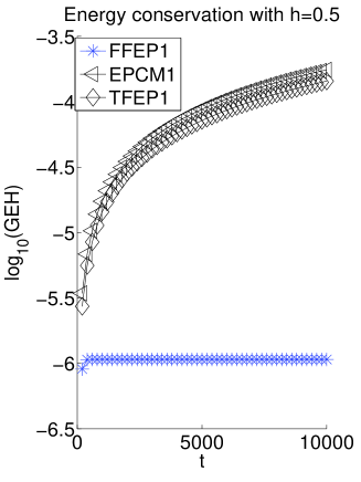
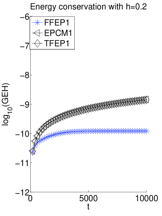
Figure 1: The logarithm of the error of Hamiltonian against $t$.

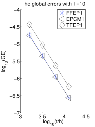
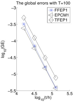
Figure 2: The logarithm of the global error against the logarithm of $t/h$.

We also consider a more anomalous case. As mentioned in [22], when $\beta\approx 1$, it is expected that $\dot{y}_{3}\approx 0$ and thus $y_{3}(t)\approx 1.$ Therefore, the variables $y_{1}$ and $y_{2}$ seem to behave like harmonic oscillator with the period $T_{p}=2\pi/(\alpha-1).$ We choose $\alpha=51$ and $\beta=1.01$, which means that $\omega=50$. We integrate this problem with $h=0.5$ and $h=0.2$ in the interval $[0,10000].$ The energy conservation for different methods are shown in Figure 3. Then the problem is solved in the interval $[0,T]$ with $h=0.1/2^{i}$ for $i=4,5,6,7,$ and see Figure 4 for the global errors of $T=10,20$.

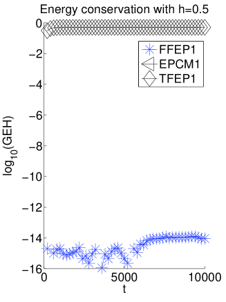
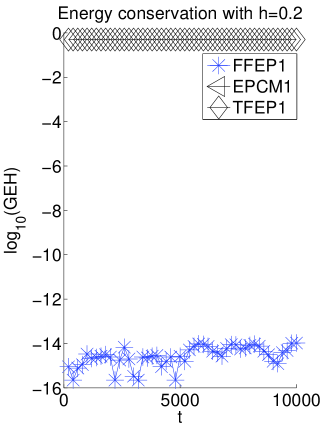
Figure 3: The logarithm of the error of Hamiltonian against $t$.

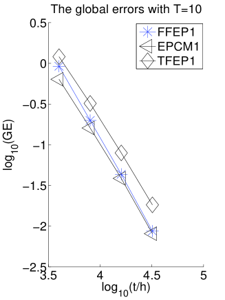
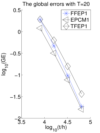
Figure 4: The logarithm of the global error against the logarithm of $t/h$.

It can be concluded from the numerical results that our FFEP1 method when applied to the underlying Euler equation shows remarkable numerical behaviour in comparison with the existing EP methods in the literature.

8 Conclusions

In this paper, we derived and analysed functionally-fitted energy-preserving integrators for Poisson systems by using functionally-fitted technology. It has been shown that the novel integrators preserve exactly the energy of Poisson systems and can be of arbitrary-order in a convenient manner. The new integrators contain the energy-preserving schemes given by Cohen and Hairer [9] and Brugnano et al. [1]. The remarkable efficiency and robustness of the integrators were demonstrated through the numerical experiments for the Euler equation. Our future work will be focused on developing functionally-fitted energy-preserving integrators for gradient systems. We are hopeful of obtaining some new results within this framework.

References

• [1] L. Brugnano, M. Calvo, J. I. Montijano, L. Rández, Energy-preserving methods for Poisson systems, J. Comput. Appl. Math. 236 (2012) 3890-3904.
• [2] L. Brugnano, F. Iavernaro, D. Trigiante, Hamiltonan Boundary Value Methods (Energy Preserving Discrete Line Integral Methods), J. Numer. Anal. Ind. Appl. Math. 5 (2010) 13-17.
• [3] L. Brugnano, F. Iavernaro, D. Trigiante, Energy- and quadratic invariants-preserving integrators based upon Gauss-Collocation formulae, SIAM J. Numer. Anal. 50 (2012) 2897-2916.
• [4] M. Calvo, J. M. Franco, J. I. Montijano, L. Rández, Sixth-order symmetric and symplectic exponentially fitted Runge–Kutta methods of the Gauss type, J. Comput. Appl. Math. 223 (2009) 387-398.
• [5] M. Calvo, J. M. Franco, J. I. Montijano, L. Rández, On high order symmetric and symplectic trigonometrically fitted Runge–Kutta methods with an even number of stages, BIT Numer. Math. 50 (2010) 3-21.
• [6] M. Calvo, J. M. Franco, J. I. Montijano, L. Rández, Symmetric and symplectic exponentially fitted Runge–Kutta methods of high order, Comput. Phys. Comm. 181 (2010) 2044-2056.
• [7] E. Celledoni, R. I. Mclachlan, B. Owren, and G. R. W. Quispel, Energy-preserving integrators and the structure of B-series, Found. Comput. Math. 10 (2010) 673-693.
• [8] E. Celledoni, B. Owren, Y. Sun, The minimal stage, energy preserving Runge–Kutta method for polynomial Hamiltonian systems is the averaged vector field method, Math. Comp. 83 (2014) 1689-1700.
• [9] D. Cohen, E. Hairer, Linear energy-preserving integrators for Poisson systems, BIT 51 (2011) 91-101.
• [10] M. Dahlby, B. Owren, T. Yaguchi, Preserving multiple first integrals by discrete gradients, J. Phys. A Math. Theo. 44 (2012) 1651-1659.
• [11] K. Feng, M. Qin, Symplectic Geometric Algorithms for Hamiltonian Systems, Springer-Verlag, Berlin, Heidelberg, 2010.
• [12] J. M. Franco, Exponentially fitted symplectic integrators of RKN type for solving oscillatory problems, Comput. Phys. Comm. 177 (2007) 479-492.
• [13] E. Hairer, Energy-preserving variant of collocation methods, J. Numer. Anal. Ind. Appl. Math. 5 (2010) 73-84.
• [14] E. Hairer, C. Lubich, Oscillations over long times in numerical Hamiltonian systems, in Highly oscillatory problems (B. Engquist, A. Fokas, E. Hairer, A. Iserles, eds.), London Mathematical Society Lecture Note Series 366, Cambridge Univ. Press, 2009.
• [15] E. Hairer, C. Lubich, Long-term analysis of the Störmer-Verlet method for Hamiltonian systems with a solution-dependent high frequency, Numer. Math. 134 (2016) 119-138.
• [16] E. Hairer, C. Lubich, G. Wanner, Geometric Numerical Integration: Structure-Preserving Algorithms for Ordinary Differential Equations, 2nd edn. Springer-Verlag, Berlin, Heidelberg, 2006.
• [17] Y.W. Li, X. Wu, Exponential integrators preserving first integrals or Lyapunov functions for conservative or dissipative systems, SIAM J. Sci. Comput. 38 (2016) 1876-1895.
• [18] Y.W. Li, X. Wu, Functionally fitted energy-preserving methods for solving oscillatory nonlinear Hamiltonian systems, SIAM J. Numer. Anal. 54 (2016) 2036-2059.
• [19] R. I. McLachlan, G. R. W. Quispel, Discrete gradient methods have an energy conservation law, Discrete Contin. Dyn. Syst. 34 (2014) 1099-1104.
• [20] R. I. McLachlan, G. R. W. Quispel, N. Robidoux, Geometric integration using discrete gradient, Philos. Trans. R. Soc. Lond. A 357 (1999) 1021-1045.
• [21] L. Mei, X. Wu, Symplectic exponential Runge-Kutta methods for solving nonlinear Hamiltonian systems, J. Comput. Phys. 338 (2017) 567-584.
• [22] Y. Miyatake, A derivation of energy-preserving exponentially-fitted integrators for Poisson systems, Comput. Phys. Comm. 187 (2015) 156-161.
• [23] Y. Miyatake, An energy-preserving exponentially-fitted continuous stage Runge–Kutta method for Hamiltonian systems, BIT Numer. Math. 54 (2014) 777-799.
• [24] G. R. W. Quispel, D. I. McLaren, A new class of energy-preserving numerical integration methods, J. Phys. A 41 (045206) (2008) 7pp.
• [25] G. Vanden Berghe, Exponentially-fitted Runge–Kutta methods of collocation type: fixed or variable knots?, J. Comput. Appl. Math. 159 (2003) 217-239.
• [26] H. Van de Vyver, A fourth order symplectic exponentially fitted integrator, Comput. Phys. Comm. 176 (2006) 255-262.
• [27] B. Wang, A. Iserles, X. Wu, Arbitrary-order trigonometric Fourier collocation methods for multi-frequency oscillatory systems, Found. Comput. Math. 16 (2016) 151-181.
• [28] B. Wang, X. Wu, A new high precision energy-preserving integrator for system of oscillatory second-order differential equations, Phys. Lett. A 376 (2012) 1185-1190.
• [29] B. Wang, X. Wu, Improved Filon type asymptotic methods for highly oscillatory differential equations with multiple time scales, J. Comput. Phys. 276 (2014) 62-73.
• [30] B. Wang, X. Wu, Arbitrary-order exponential energy-preserving collocation methods for solving conservative or dissipative systems, Preprint (2017) https://na.uni-tuebingen.de/preprints.shtml
• [31] B. Wang, X. Wu, F. Meng, Trigonometric collocation methods based on Lagrange basis polynomials for multi-frequency oscillatory second-order differential equations, J. Comput. Appl. Math. 313 (2017) 185-201.
• [32] B. Wang, H. Yang, F. Meng, Sixth order symplectic and symmetric explicit ERKN schemes for solving multi-frequency oscillatory nonlinear Hamiltonian equations, Calcolo 54 (2017) 117-140.
• [33] X. Wu, K. Liu, W. Shi, Structure-preserving algorithms for oscillatory differential equations II, Springer-Verlag, Heidelberg, 2015.
• [34] X. Wu, B. Wang, W. Shi, Efficient energy preserving integrators for oscillatory Hamiltonian systems, J. Comput. Phys. 235 (2013) 587-605.
• [35] X. Wu, B. Wang, J. Xia, Explicit symplectic multidimensional exponential fitting modified Runge-Kutta-Nyström methods, BIT 52 (2012) 773-795.
• [36] X. Wu, X. You, B. Wang, Structure-preserving algorithms for oscillatory differential equations, Springer-Verlag, Berlin, Heidelberg, 2013.