Axion inflation, proton decay, and leptogenesis in $SU(5)\times U(1)_{PQ}$

Abstract

We implement inflation in a non-supersymmetric $SU(5)$ model based on a non-minimal coupling of the axion field to gravity. The isocurvature fluctuations are adequately suppressed, axions comprise the dark matter, proton lifetime estimates are of order $8\times 10^{34}-3\times 10^{35}$ yr, and the observed baryon asymmetry arises via non-thermal leptogenesis. The presence of low scale colored scalars ensures unification of the Standard Model gauge couplings and also helps in stabilizing the electroweak vacuum.

I Introduction

Successful inflation models based on $SU(5)$ grand unified theory (GUT) and employing a Coleman-Weinberg potential with minimal coupling to gravity were constructed some time ago ShafiVilenkinSU5 and, for values of the scalar spectral index $n_{s}\sim 0.96-0.97$, the tensor to scalar ratio $r$ is $\gtrsim 10^{-2}$ Rehman:2008qs . In these models the inflaton field, an $SU(5)$ gauge singlet, evolves from the origin to its non-zero vev, reaching trans-Planckian values near its minimum during the last 60 or so e-foldings. Identifying the $SU(5)$ gauge singlet inflaton with the axion Wilczek:1977pj ; Weinberg:1977ma field is very attractive and was first done in Pi:1984pv . However, it turns out to be not very compelling for this model because of the excessively large value $f_{a}\sim 10^{19}$ GeV imposed on the axion decay constant by inflation Rehman:2008qs . Typically, an axion decay constant $f_{a}\sim 10^{11-12}$ GeV is the desired value for axion dark matter.

It has been known for a while that primordial inflation driven by a scalar quartic potential and based on non-minimal coupling to gravity is fully consistent with the Planck observations Okada:2014lxa for plausible values, say $\xi\lesssim 10$, of the dimensionless non-minimal coupling parameter $\xi$. The inflaton field in this case rolls down from trans-Planckian values to its final minimum which can be sub-Planckian as desired. The scalar quartic coupling $\lambda$ during inflation in this case turns out to be $\lesssim 10^{-8}$. This means that in order to protect $\lambda$ from unacceptably large radiative corrections, in non-supersymmetric GUTs the inflaton should again be identified with a gauge singlet scalar field, as was done in the $SU(5)$ model mentioned above.

An axion model needed to resolve the strong CP problem provides a compelling candidate to implement successful inflation in GUTs using non-minimal coupling to gravity. For the sake of simplicity, we will employ a Higgs rather than the Coleman-Weinberg potential. The inflaton (radial component of the axion field) in this case rolls down from trans-Planckian values during inflation to its final value $f_{a}\sim 10^{11-12}$ GeV, thus yielding a viable scenario with axion dark matter.

With trans-Planckian field values during inflation the isocurvature fluctuations are adequately suppressed and observable gravity waves corresponding to $r\sim\mathrm{few}\times 10^{-3}$ are predicted. The reheating process proceeds via the decay of the inflaton into right-handed (RH) neutrinos. In turn, the latter yield the observed baryon asymmetry via non-thermal leptogenesis.

The realistic GUT model we propose successfully addresses several problems of the SM at once, namely the existence and nature of dark matter, the strong CP problem, baryogenesis, the stability of the electroweak vacuum, the origin of the inflationary phase, and the physics behind neutrino masses. All of these issues have been previously studied in the literature in the aim of providing unified schemes which tackle several of them simultaneously, see e.g., Refs Langacker:1986rj ; Shin:1987xc ; Davoudiasl:2004be ; Shaposhnikov:2006xi ; Boucenna:2014uma ; Bertolini:2014aia ; Clarke:2015bea ; Ahn:2015pia ; Salvio:2015cja ; Ballesteros:2016euj . Here we show that a simple non-supersymmetric GUT model provides an elegant framework to solve all these problems, in addition to providing matter and gauge coupling unification.

This letter is organized as follows. We describe our model and outline its most salient features in Sec. (II). We then analyse the constraints on gauge coupling unification (GCU) and proton decay in Sec. (III). These end up predicting the presence of a colored octet scalar not far from the TeV scale. Such a field also plays a critical role in stabilizing the electroweak vacuum which we analyse in Sec. (IV). After which we outline the main features of inflation based on a quartic potential with non-minimal coupling of the inflaton field to gravity in Sec. (V), and derive the predictions for the spectral index $n_{s}$, the scalar-to-tensor ratio $r$, and the running of the spectral index $\alpha$. We also present constraints on the magnitude of Yukawa couplings involving RH neutrinos and estimate the reheat temperature taking into account the requirement of axion dark matter. Next, in in Sec. (VI) we describe how leptogenesis is implemented in this framework. Finally, in Sec. (VII) we show how the inflaton coupling to the adjoint $\mathbf{24}$-plet insures $SU(5)$ breaking during inflation so that the superheavy monopoles are inflated away.

	$T_{L}$	$F_{L}$	$\nu_{L}^{c}$	$H_{1}$	$H_{2}$	$\sigma$	$\Phi$	$\chi$
$SU(5)$	$\mathbf{10}$	$\mathbf{\overline{5}}$	$\mathbf{1}$	$\mathbf{5}$	$\mathbf{\overline{5}}$	$\mathbf{1}$	$\mathbf{24}$	$\mathbf{45}^{\star}$
$U(1)_{PQ}$	$q/2$	$q/2$	$q$/2	$-q$	$-q$	$-q$	0	$-q$
$U(1)_{X}$	$1/5$	$-3/5$	$-1$	$-2/5$	$2/5$	$2$	0	$2/5$

Table 1: Summary of the quantum numbers of the different fields of the model. $q$ is an arbitrary number. $U(1)_{X}$ is an accidental symmetry of the model when the mixed term $(\sigma^{\star})^{2}H_{1}H_{2}$ is absent, i.e., in the limit $\lambda_{\nu}\to 0$.

II The model

The model consists of a simple extension of the original $SU(5)$ model Georgi:1974sy . The SM fermion fields are in the usual $\mathbf{10}$ ($T_{L}$) and $\mathbf{\overline{5}}$ ($F_{L}$), and we add the singlet RH neutrinos $\nu_{L}^{c}$. The scalar sector of the model involves $\mathbf{5}$ ($H_{1}$), $\mathbf{5^{\star}}$ ($H_{2}$), $\mathbf{24}$ ($\Phi$), and lastly $\mathbf{45}^{\star}$ ($\chi$, with $\chi^{ij}_{k}=-\chi^{ji}_{k}$ for $i,j,k=1-5$). In addition, we define a global $U(1)_{PQ}$ symmetry to implement the Peccei-Quinn (PQ) mechanism Peccei:1977ur solving the strong CP problem and providing an invisible axion via the DFSZ mechanism Zhitnitsky:1980tq ; Dine:1981rt ; see Table (1) for the $U(1)_{PQ}$ charges of the different fields.

The relevant terms in the scalar potential of the model read:

$$V \supset -\tfrac{1}{2}M_{GUT}^{2}\mathrm{{Tr}}(\Phi^{2})-M_{\sigma}^{2}\sigma\sigma^{\star}+\lambda_{\sigma}(\sigma^{\star}\sigma)^{2}$$ (1)

$$+\sigma\sigma^{\star}\sum_{\phi}\kappa_{\phi}\phi^{\star}\phi+\lambda_{\nu}[(\sigma^{\star})^{2}H_{1}H_{2}+\mathrm{h.c.}]\,.$$

Here $\phi=(H_{1},H_{2},\Phi,\chi)$ and the dot product $\phi^{\star}.\phi$ represents the $SU(5)\times U(1)_{PQ}$ invariant contractions. And the Yukawa part of the Lagrangian is given by the following terms (family, gauge, and Lorentz indices are suppressed):

$$\mathcal{L}_{Yuk} = T_{L}.\mathbf{Y_{10}}.T_{L}.H_{1}+T_{L}.\mathbf{Y_{5}}.F_{L}.H_{2}+T_{L}.\mathbf{Y_{45}}.F_{L}.\chi\,$$ (2)

$$F_{L}.\mathbf{Y_{\nu}}.\nu_{L}^{c}.H_{1}+\tfrac{1}{2}\mathbf{Y_{N}}\nu_{L}^{c}.\nu_{L}^{c}.\sigma+\mathrm{h.c.}\,,$$

where $\mathbf{Y}_{i}$ are dimensionless $3\times 3$ matrices. The PQ symmetry is tightly related to lepton number in this scheme. We can readily see that if $\lambda_{\nu}=0$, the Lagrangian is invariant under $U(1)_{B-L}$ symmetry after the breaking of $SU(5)$ and $U(1)_{PQ}$. Indeed, an accidental $U(1)_{X}$ symmetry (shown in Table (1)) combines with the usual hypercharge to leave an unbroken $U(1)$ defined by $X+\tfrac{4}{5}Y\equiv B-L$. However, this symmetry is explicitely broken in the scalar sector due to the presence of the $\lambda_{\nu}$ term which is crucial for generating the axion in the DFSZ model and cannot be set to zero. Additionally, $\lambda_{\nu}\neq 0$ allows us to get rid of the majoron goldstone boson Chikashige:1980ui ; Gelmini:1980re since lepton number is broken explicitely Langacker:1986rj .

The representations involved in the model play crucial roles in different phenomenological sectors. Namely,

• $H_{1,2}$ and $\chi$ account for the SM charged fermion masses and mixings in a renormalizable way. The two-Higgs-Doublet model (2-HDM) consisting of $H_{1,2}$ ensures the implementation of the DFSZ mechanism. The multiplet $\chi$ is also crucial for obtaining accurate gauge coupling unification;

• $\left\langle\Phi\right\rangle$ breaks $SU(5)$ to the SM;

• the phase of $\sigma$ is the axion which solves the strong CP problem and accounts for the DM of the universe, and the radial part drives inflation;

• $\left\langle\sigma\right\rangle$ provides large Majorana masses for $\nu_{L}^{c}$ via the see-saw mechanism. After inflation the latter helps generate the observed baryon asymmetry via non-thermal leptogenesis.

In the next sections we will investigate in details all these aspects of the model.

III Fermions masses, gauge coupling unification, and proton decay

From eq. (2), we obtain the following mass relations:

$$M_{e} = \mathbf{Y_{5}}^{T}\left\langle H_{2}\right\rangle-6\mathbf{Y_{45}}^{T}\left\langle\chi\right\rangle$$ (3)

$$M_{d} = \mathbf{Y_{5}}\left\langle H_{2}\right\rangle+2\mathbf{Y_{45}}\left\langle\chi\right\rangle$$ (4)

$$M_{u} = 4(\mathbf{Y_{10}}+\mathbf{Y_{10}}^{T})\left\langle H_{1}\right\rangle$$ (5)

$$M_{\nu} \simeq \mathbf{Y_{\nu}}^{T}.\mathbf{Y_{N}}^{-1}.\mathbf{Y_{\nu}}\tfrac{\left\langle H_{1}\right\rangle^{2}}{\left\langle\sigma\right\rangle}\,.$$ (6)

In the last equation we have assumed the see-saw scaling $\left\langle\sigma\right\rangle\gg\left\langle H_{1}\right\rangle$ for natural couplings. We define $\left\langle\chi\right\rangle\equiv\left\langle\chi\right\rangle^{15}_{1}=\left\langle\chi\right\rangle^{25}_{2}=\left\langle\chi\right\rangle^{35}_{3}=-3\left\langle\chi\right\rangle^{45}_{4}$. It is clear from these expressions that there is enough parameter freedom to fit the fermion masses and cure the wrong predictions of minimal $SU(5)$ Georgi:1979df ; Kalyniak:1982pt ; Eckert:1983bn .

Next, we turn to the issue of gauge coupling unification (GCU). In the minimal $SU(5)$ model, the gauge couplings do not properly unify at high energy. However, the $\chi$ and $\Phi$ multiplets contain representations which can alter the renormalization group (RG) evolution in a favourable way Dorsner:2006dj . In particular, we will use $R_{8}\equiv(\mathbf{8},\mathbf{2},1/2)\in\chi$ and $R_{3}\equiv(\mathbf{3},\mathbf{3},-1/3)\in\chi$ to obtain precise GCU. Note that in the absence of the PQ symmetry $R_{3}$ can mediate proton decay leading to a lower limit on its mass that was estimated to be around $10^{10}$ GeV  Dorsner:2006dj . However, in our scenario $R_{3}$ cannot induce nucleon decay due to the absence of the couplings $T_{L}.\chi.H_{2}$ or $T_{L}.\chi.H_{1}^{\star}$ and thus it can be very light. This significantly enlarges the parameter space consistent with GCU.

We solve the system of RG equations in order to obtain successful GCU. The equations depend on 3 parameters: $M_{R_{3}}$, $M_{R_{8}}$, and $M_{GUT}$ (for simplicity, we ignore threshold effects). We require that $M_{GUT}$ is large enough so that gauge-mediated proton decay does not rule out the model, i.e.,

$$\tau_{p}\sim\alpha_{GUT}^{-2}\frac{M_{GUT}^{4}}{m_{p}}\gtrsim 10^{34}\,\mathrm{yr}\,,$$ (7)

where $m_{p}$ is the proton mass and the lower limit is the current experimental bound on $\tau_{p}(p\to e^{+}\pi^{0})$PDG2016 . After combining these constraints, we find:

$$M_{GUT} \approx \left(\frac{M_{R_{8}}}{\mathrm{TeV}}\right)^{-0.126}\times 10^{16}\,\mathrm{GeV}\,,$$ (8)

$$M_{R_{3}} \approx \left(\frac{M_{R_{8}}}{\mathrm{TeV}}\right)^{0.05}\times 6.1\times 10^{7}\,\mathrm{GeV}\,,$$ (9)

and

$$M_{R_{8}} \lesssim 6\times 10^{5}\,\mathrm{GeV}\,.$$ (10)

The maximum proton lifetime is achieved for the smallest possible $R_{8}$ mass. For 1 TeV mass, we obtain $\tau_{p}\approx 2.4\times 10^{35}$ yr, which is around the expected sensitivity of Hyper-Kamiokande experiment Abe:2011ts . We display the gauge coupling unification in Figure (1) for the case where $M_{R_{8}}=1$ TeV.

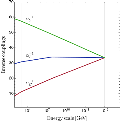
Figure 1: Evolution of the inverse coupling strengths with energy. Here $M_{R_{8}}=1$ TeV, $M_{R_{3}}\approx 6.1\times 10^{7}$ GeV, and $M_{GUT}\approx 10^{16}$ GeV. The proton lifetime in this case is $\tau_{p}\approx 2.4\times 10^{35}$ yr.

IV Vacuum stability

It is well known that that the vacuum instability problem associated with the quartic coupling of the Higgs (see for instance Buttazzo:2013uya ) can be overcome with new physics around the TeV scale. The GCU analysis in the previous section revealed that the model predicts scalar representations which have to be lighter than $\sim 10^{10}$ GeV, more or less the scale at which the quartic coupling becomes negative. This is remarkable as such scalars will contribute to the running of the quartic coupling and could positively tilt it before it becomes negative. In this section we will analyse the effect of these scalars on the stability of the vacuum. For renormalization energy $\mu<M_{R_{8}}$, we use the SM RG equations at two-loop level to calculate the evolution of the Higgs quartic coupling Machacek:1983tz ; Machacek:1984zw ; Ford:1992pn ; Arason:1991ic ; Barger:1992ac ; Luo:2002ey . We include the effects from the new particles $R_{3}$ and $R_{8}$ at one-loop level. These modify the first order coeffcients $b_{i}$ of the SM, $\tfrac{dg_{i}}{dln\mu}=\tfrac{b_{i}}{16\pi^{2}}g_{i}^{3}$, $b_{i}(\mu)=(\tfrac{41}{10},-\tfrac{19}{6},-7)+\Theta(\mu-M_{R_{8}})(2,\tfrac{4}{3},\tfrac{4}{5})+\Theta(\mu-M_{R_{3}})(\tfrac{1}{2},2,\frac{1}{5})$. In solving the RGEs, we use the boundary conditions at the top quark pole mass given in Buttazzo:2013uya . For the $SU(3)_{c}$ coupling constant and the top mass, we use $\alpha_{s}=0.1184$ and $M_{t}=173.34$ GeV ATLAS:2014wva respectively. The SM Higgs mass is fixed at $M_{h}=125.09$ GeV Aad:2015zhl . We find in particular that $R_{8}$, being very light, induces a significant effect on the running of the gauge couplings. The scalar $R_{3}$ on the other hand has a negligible effect on the running before the instability scale. As we can see in Figure (2), the quartic Higgs coupling is indeed prevented from becoming negative by including the $R_{8}$ field at 1 TeV and $R_{3}$ at $6.1\times 10^{7}$ GeV. Remarkably, the same fields which alllow us to implement GCU also stabilise the effective potential of the SM at high energies.

Finally, we can use this analysis to constrain the mass of $R_{8}$. Indeed, the heavier it is the less important is its effect on the Higgs quartic coupling, and so we expect an upper bound not far from the TeV region. We find that

$$M_{R_{8}} \lesssim 10^{4}\,\mathrm{GeV}\,,$$ (11)

which is more constraining than the upper bound derived from GCU considerations only. Using eq. (8), this upper bound translates as $\tau_{p}\gtrsim 7.8\times 10^{34}$ yr.

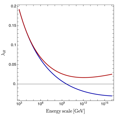
Figure 2: Vacuum stability of the Higgs potential. The red (upper) line shows the running of the Higgs quartic coupling in the model compatible with Figure (1). We display in blue (lower line) its running in the SM for comparison.

V Axion Inflation

We assume that inflation is driven by the radial part of the complex singlet $\sigma$, $\rho\equiv\sqrt{{2}}\mathcal{{R}}e(\sigma)$. Without loss of generality, we take $\mathbf{Y_{N}}~{}=~{}\mathrm{diag(Y_{N_{1}},Y_{N_{2}},Y_{N_{3}})}$, with $Y_{N_{i}}$ real and positive. The relevant terms of the Lagrangian of the model are:

$$\mathcal{{L}}_{inf} = \left(\sum_{i=1}^{3}\frac{Y_{N_{i}}}{2\sqrt{2}}\,\rho\,{\nu_{iL}^{c}}\nu_{iL}^{c}+h.c.\right)-V_{inf}\,,$$ (12)

$$V_{inf} = \tfrac{1}{4}\lambda_{\sigma}(\rho^{2}-f_{a}^{2})^{2}+\tfrac{1}{2}\rho^{2}\sum_{\phi}\kappa_{\phi}\phi^{\star}.\phi\,,$$ (13)

where $f_{a}\equiv\sqrt{2}\left\langle\sigma\right\rangle$ and for simplicity, we only consider real couplings. We enforce $\kappa_{H_{1,2}}>0$ to ensure that inflation is driven by $\rho$. The couplings of the inflaton with $\nu_{L}^{c}$ and the scalar fields induce quantum corrections that can have significant effects on the inflationary observables. These effects induce an additional contribution to the potential $V_{inf}$ denoted as $V^{(1)}$,

$$V^{(1)}=\frac{\beta}{16\pi^{2}}\,\rho^{4}\mathrm{ln}\frac{\rho^{2}}{\mu^{2}}\,,$$ (14)

where Okada:2013vxa

$$\beta=20\lambda_{\sigma}^{2}+2\sum_{\phi}\kappa_{\phi}^{2}+2\lambda_{\sigma}\sum y_{Ni}^{2}-\sum y_{Ni}^{4}\,.$$

We require that these radiative corrections are not significant, i.e., $|\beta|\ll(16\pi^{2})|\lambda_{\sigma}|$. The most conservative limit we can set on the couplings is (defining max($Y_{N_{i}})=Y_{N}$):

$$y_{N}\lesssim 6\times 10^{-2}\,\left(\frac{\lambda_{\sigma}}{10^{-7}}\right)^{\tfrac{1}{4}}\,.$$ (15)

For the rest of the paper we will suppose that $\kappa_{\phi}\ll y_{N}$ and impose eq. (15).

V.1 $\rho^{4}$ inflation with non-minimal coupling to gravity

We consider a scenario where $\rho$ has a non-minimal coupling to gravity. For simplicity, we assume that all other scalars, including the SM Higgs, have quasi-minimal couplings. In the Jordan frame, the action of non-minimal $\rho^{4}$ inflation is given by:

$$S_{J}^{{\rm tree}}=\int d^{4}x\sqrt{-g}\left[-\left(\frac{1}{2}(1+\xi\rho^{2})\right)\mathcal{R}+\frac{1}{2}(\partial\rho)^{2}-\frac{\lambda_{\sigma}}{4}\rho^{4}\right]\,.$$ (16)

In the Einstein frame one finds,

$$S_{E}=\int d^{4}x\sqrt{-g_{E}}\left[-\frac{1}{2}\mathcal{R}_{E}+\frac{1}{2}(\partial S)^{2}-V_{E}(S(\rho))\right]\,,$$ (17)

where the canonically normalized scalar field $S$ is written in terms of the original scalar as:

$$\left(\frac{dS}{d\rho}\right)^{-2}=\frac{\left(1+\xi\rho^{2}\right)^{2}}{1+(6\xi+1)\xi\rho^{2}}\,.$$ (18)

The inflation potential now reads:

$$V_{E}(S(\rho))=\frac{\frac{1}{4}\lambda_{\sigma}(t)\rho^{4}}{\left(1+\xi\,\rho^{2}\right)^{2}}\,,$$ (19)

and the inflationary slow-roll parameters Liddle:1992wi ; Liddle:1993fq in terms of $\rho$ are expressed as:

$$\epsilon(\rho) = \frac{1}{2}\left(\frac{V_{E}^{\prime}}{V_{E}S^{\prime}}\right)^{2},$$

$$\eta(\rho) = \frac{V_{E}^{\prime\prime}}{V_{E}(S^{\prime})^{2}}-\frac{V_{E}^{\prime}S^{\prime\prime}}{V_{E}(S^{\prime})^{3}},$$

$$\frac{\zeta(\rho)}{\sqrt{2\epsilon(\rho)}} = \frac{V_{E}^{\prime\prime\prime}}{V_{E}(S^{\prime})^{3}}-\frac{3V_{E}^{\prime\prime}S^{\prime\prime}}{V_{E}(S^{\prime})^{4}}+\frac{3V_{E}^{\prime}(S^{\prime\prime})^{2}}{V_{E}(S^{\prime})^{5}}-\frac{V_{E}^{\prime}S^{\prime\prime\prime}}{V_{E}(S^{\prime})^{4}}\,,$$

where a prime denotes derivative with respect to $\rho$, and we use units where the reduced Planck mass, $M_{\mathrm{Pl}}\simeq 2.4\times 10^{18}$ GeV, is equal to unity unless otherwise stated. The number of e-folds is given by:

$$N=\frac{1}{\sqrt{2}}\int_{\rho_{{\rm e}}}^{\rho_{0}}\frac{d\rho}{\sqrt{\epsilon(\rho)}}\left(\frac{dS}{d\rho}\right)\,.$$ (20)

The inflationary predictions for the scalar spectral index $n_{s}$, the tensor-to-scalar ratio $r$, and the running of the spectral index $\alpha=\tfrac{\mathrm{d}n_{s}}{\mathrm{dln}k}$ are obtained after fixing $N$ and $\xi$. The quartic coupling $\lambda_{\sigma}$ can be fixed using the amplitude of density perturbations at some pivot scale Ade:2015lrj ,

$$\Delta_{\mathcal{{R}}}^{2}=\left.\frac{V_{E}}{24\pi^{2}\epsilon}\right|_{k^{\star}}=\left.2.196\times 10^{-9}\right|_{0.05\mathrm{{Mpc}^{-1}}}\,.$$ (21)

In Figure (3) we show the predicted values of the quartic coupling as a function of the minimal coupling $\xi$ for $N=50$ and $N=60$ e-foldings. $n_{s}$ is constrained to be within the 68% confidence level of Planck’s measurement Ade:2015lrj .

For $\xi\gtrsim 0.1$, the predicted values of $n_{s}$, $r$, and $\alpha$ quickly converge toward:

	$n_{s}$	$r\times 10^{3}$	$-\alpha\times 10^{4}$
$N=50$	$0.962$	$4$	$7.5$
$N=60$	$0.968$	$3$	$5.3$

This implies that the Hubble expansion rate at the end of inflation is:

$$H_{I}\simeq 2\pi\times 10^{13}\;\mathrm{{GeV}\,}\,.$$ (22)

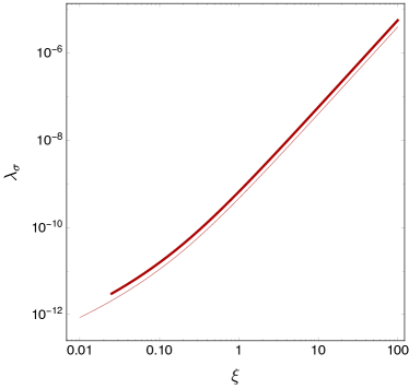
Figure 3: Correlation between the inflaton’s quartic coupling $\lambda_{\sigma}$ and the non-minimal coupling $\xi$ for $N=50$ e-foldings (thick line) and $N=60$ e-foldings (thin line). $n_{s}$ is within the 68% confidence level of Planck’s measurement.

V.2 Reheating

As can be seen in eq. (15), the coupling of the inflaton with $\nu^{c}_{L}$ can be sizable, and this can be used to reheat the Universe via the decays $\rho\to 2\nu^{c}_{L}$. This is the dominant process because our assumption that $\kappa_{\phi}\ll 1$ makes reheating via the scalars inefficient. In order to do so, the mass of at least one of RH neutrinos $M_{N}=y_{N}\,f_{a}/\sqrt{2}$ must be smaller than half the inflaton’s mass $m_{\rho}=B\,f_{a}$, with $B\simeq\sqrt{2\lambda_{\sigma}}$. This translates as:

$$y_{N}<\sqrt{2\lambda_{\sigma}}\,.$$ (23)

Note that this condition is more stringent than the one obtained in eq. (15). Assuming an instantaneous conversion of the inflaton’s energy density into radiation, at the time when $H(t)\approx\Gamma_{\rho}$ (decay rate of $\rho$), we can define the reheating temperature as:

$$T_{RH}=\left(\frac{45}{4\pi^{3}g_{\star}}\right)^{1/4}\sqrt{\Gamma_{\rho}}\sim 0.1\sqrt{\Gamma_{\rho}}\,,$$ (24)

where

$$\Gamma_{\rho}=\frac{3\>y_{N}^{2}}{64\pi}m_{\rho}\,.$$ (25)

Using eq. (23) we can derive the bound

$$T_{RH}\lesssim 3\times 10^{8}\,\mathrm{GeV}\sqrt{\left(\frac{\lambda_{\sigma}}{10^{-7}}\right)\left(\frac{f_{a}}{10^{12}\>\mathrm{GeV}}\right)}\equiv T_{RH}^{\mathrm{{max}}}\,.$$ (26)

V.3 Non-adiabatic primordial fluctuations of axions

Since inflation is driven by the radial part of the axion field, the PQ symmetry is always broken during inflation and the axion acquires isothermal (more precisely isocurvature) fluctuations Axenides:1983hj ; Linde:1985yf ; Linde:1991km ; Linde:1984ti ; Seckel:1985tj ; Turner:1990uz . In general, these are given by Fairbairn:2014zta

$$\beta_{\mathrm{iso}}=\left(1+\frac{\pi f_{a,\star}^{2}\overline{\theta_{i}^{2}}}{\epsilon(\rho)}\right)^{-1}\leq 0.038\,,$$ (27)

with $f_{a,\star}$ being the effective scale of PQ symmetry breaking and $\overline{\theta_{i}}$ is the spatially averaged misalignment angle. The upper bound is the current experimental limit (95% confidence level) at $k=0.05$ Mpc^-1 Ade:2015lrj . Assuming that axion DM is produced via the misalignment mechanism Preskill:1982cy ; Abbott:1982af ; Dine:1982ah , $\overline{\theta_{i}}$ enters as well in the expression of the axion relic density:

$$\Omega_{a}h^{2}=0.1199\>\left(\frac{\overline{\theta_{i}^{2}}}{0.28}\right)\left(\frac{f_{a}}{10^{12}\,\mathrm{GeV}}\right)^{7/6}\,.$$ (28)

In the standard scenario where inflation is unrelated to axions $f_{a,\star}\equiv f_{a}$, and the bound eq. (27) favors a large PQ breaking scale. However in our case the effective scale is given by the inflaton field value during inflation, $\rho_{\star}$, which is trans-Planckian for $\xi\lesssim 10^{2}$. Given that $\rho_{\star}\gg f_{a}$, $f_{a}$ does not have a direct impact on the isocurvature perturbations and enters only indirectly via eq. (28). Using eqs. (27) and ( 28) we obtain un upper bound on $f_{a}$ for a given $\xi$. In Figure (4) we depict the predicted values of the maximal allowed value of $f_{a}$ as a function of the minimal coupling $\xi$ for $N=50$ and $N=60$ e-foldings. As in Figure (3), $n_{s}$ is constrained to be within the 68% confidence level of Planck’s measurement Ade:2015lrj . The obtained limit on $f_{a}$ is compatible with the natural parameter space of axion DM. Finally, note that for our choice of parameters, namely $f_{a}\sim 10^{12}$ GeV, the PQ symmetry is not restored at the end of reheating since $T_{RH}\ll f_{a}$, see eq. (26).

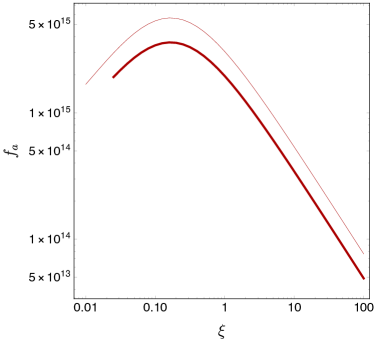
Figure 4: Upper bound on the PQ scale $f_{a}$ as a function of the non-minimal coupling $\xi$ due to isocurvature and DM relic abundance constraints. The two lines are for for $N=50$ e-foldings (thick) and $N=60$ e-foldings (thin). $n_{s}$ is within the 68% confidence level of Planck’s measurement.

VI Baryogenesis

In eq. (26) we found that the maximum reheat temperature obtained from inflaton’s decays to RH neutrinos is of order $10^{8}-10^{9}$ GeV. This allows us to implement baryogenesis via non-thermal leptogenesis Lazarides:1991wu . Assuming hierarchical RH neutrino masses, the lepton-to-entropy ratio Asaka:1999yd is given by

$$\eta_{L}\simeq-10^{-5}\left(\frac{T_{RH}}{10^{9}\,\mathrm{GeV}}\right)\left(\frac{M_{N}}{m_{\rho}}\right)\,,$$ (29)

and the observed baryon asymmetry is related to $\eta_{L}$ via the usual relation $\eta_{B}\simeq 10^{-10}\simeq-\tfrac{8}{23}\eta_{L}$. This leads to

$$M_{N}\simeq 0.3\left(\frac{10^{7}\,\mathrm{GeV}}{T_{RH}}\right)m_{\rho}\,.$$ (30)

Since $m_{\rho}\simeq Bf_{a}$, we find that for $\xi\sim 1$ and $T_{RH}\sim 10^{7}$ GeV, the heavy RH neutrino with mass of the order of $10^{8}$ GeV can give rise to the observed baryon asymmetry via non-thermal leptogenesis.

VII GUT Monopoles

The $SU(5)$ symmetry breaks to the SM when the effective mass squared term of $\Phi$, $-M_{GUT}^{2}+\kappa_{\Phi}\rho^{2}$, in the effective potential becomes of order $-T_{H}^{2}$, with $T_{H}$ being the Hawking-Gibbons temperature, $T_{H}\equiv H/(2\pi)$. We want to make sure that $\Phi$ is pushed away from its origin during inflation. This must occur at the early stage of inflation to ensure that monopoles are adequately inflated away ShafiVilenkinSU5 . In the limit $\kappa_{\Phi}\to 0$, this translates as a lower bound on the unification scale,

$$M_{GUT}>(1+\xi\rho_{i}^{2})T_{H}\,.$$ (31)

where $\rho_{i}$ is the starting value of the inflaton field. $\xi\rho_{i}^{2}$ varies from $\approx 0$ to $\approx 70$ in the range $\xi\in[0,100]$. Using the result in eq. (22), we find that the equation above yields $M_{GUT}\gtrsim 7\times 10^{14}$ GeV, which is less constraining than the limit from proton lifetime. If $\kappa_{\Phi}<0$ then this condition is even easier to satisfy. However, in the case where $\kappa_{\Phi}>0$ we will have an upper limit on $\kappa_{\Phi}$ to ensure that $(M_{GUT}^{2}-|\kappa_{\Phi}|\rho_{i}^{2})>T_{H}^{2}$ and monopoles are properly inflated away. For realistic $M_{GUT}$ values, we find that $\kappa_{\Phi}\lesssim 10^{-7}$ for $\xi=10^{-2}$ and $\kappa_{\Phi}\lesssim 10^{-5}$ for $\xi=10^{2}$, which is in agreement with our initial assumptions on the smallness of $\kappa_{\phi}$.

VIII Summary and conclusions

We have presented a realistic grand unified theory based on $SU(5)\times U(1)_{PQ}$ which consistently addresses multiple outstanding BSM problems. Fermion masses and mixings are accounted for in a renormalizable fashion, and precise gauge coupling unification is achieved. With the unification scale predicted to lie around $10^{16}$ GeV, proton lifetime is predicted to be in the range $8\times 10^{34}-3\times 10^{35}$ yr and should be accessible in the next generation detectors. The effective Higgs potential is automatically stabilized thanks to the physics used to implement gauge coupling unification.

The QCD axion is our candidate for the dark matter in the universe. The axion field plays several roles in our model. The radial component of the axion field drives inflation by exploiting a non-minimal coupling to gravity, reheating proceeds from the axion field coupling to RH neutrinos, and the observed baryon asymmetry arises via non-thermal leptogenesis. The coupling with RH neutrinos inducing small neutrino masses via the see-saw mechanism. The isocurvature fluctuations are adequately suppressed and the axion decay constant $f_{a}$ lies in the desired range of $10^{11}-10^{12}$ GeV. The model predicts a tensor to scalar $r$ in an observable range, $r=\mathrm{few}\times 10^{-3}$. We finally comment that the discussion can be extended to realistic $SO(10)$ models with a suitable intermediate scale such as $SU(4)\times SU(2)\times SU(2)$ or $SU(3)\times SU(2)\times SU(2)\times U(1)$.

References

- (1) Q. Shafi and A. Vilenkin, “Inflation with SU(5),” Phys. Rev. Lett. 52 (1984) 691–694.
- (2) M. U. Rehman, Q. Shafi, and J. R. Wickman, “GUT Inflation and Proton Decay after WMAP5,” Phys. Rev. D78 (2008) 123516, arXiv:0810.3625 [hep-ph].
- (3) F. Wilczek, “Problem of Strong P and T Invariance in the Presence of Instantons,” Phys. Rev. Lett. 40 (1978) 279–282.
- (4) S. Weinberg, “A New Light Boson?,” Phys. Rev. Lett. 40 (1978) 223–226.
- (5) S.-Y. Pi, “Inflation Without Tears,” Phys. Rev. Lett. 52 (1984) 1725–1728.
- (6) N. Okada, V. N. Şenoğuz, and Q. Shafi, “The Observational Status of Simple Inflationary Models: an Update,” Turk. J. Phys. 40 no. 2, (2016) 150–162, arXiv:1403.6403 [hep-ph].
- (7) P. Langacker, R. D. Peccei, and T. Yanagida, “Invisible Axions and Light Neutrinos: Are They Connected?,” Mod. Phys. Lett. A1 (1986) 541.
- (8) M. Shin, “Light Neutrino Masses and Strong CP Problem,” Phys. Rev. Lett. 59 (1987) 2515. [Erratum: Phys. Rev. Lett.60,383(1988)].
- (9) H. Davoudiasl, R. Kitano, T. Li, and H. Murayama, “The New minimal standard model,” Phys. Lett. B609 (2005) 117–123, arXiv:hep-ph/0405097 [hep-ph].
- (10) M. Shaposhnikov and I. Tkachev, “The nuMSM, inflation, and dark matter,” Phys. Lett. B639 (2006) 414–417, arXiv:hep-ph/0604236 [hep-ph].
- (11) S. M. Boucenna, S. Morisi, Q. Shafi, and J. W. F. Valle, “Inflation and majoron dark matter in the seesaw mechanism,” Phys. Rev. D90 no. 5, (2014) 055023, arXiv:1404.3198 [hep-ph].
- (12) S. Bertolini, L. Di Luzio, H. Kolešová, and M. Malinský, “Massive neutrinos and invisible axion minimally connected,” Phys. Rev. D91 no. 5, (2015) 055014, arXiv:1412.7105 [hep-ph].
- (13) J. D. Clarke and R. R. Volkas, “Technically natural nonsupersymmetric model of neutrino masses, baryogenesis, the strong CP problem, and dark matter,” Phys. Rev. D93 no. 3, (2016) 035001, arXiv:1509.07243 [hep-ph]. [Phys. Rev.D93,035001(2016)].
- (14) Y. H. Ahn and E. J. Chun, “Minimal Models for Axion and Neutrino,” Phys. Lett. B752 (2016) 333–337, arXiv:1510.01015 [hep-ph].
- (15) A. Salvio, “A Simple Motivated Completion of the Standard Model below the Planck Scale: Axions and Right-Handed Neutrinos,” Phys. Lett. B743 (2015) 428–434, arXiv:1501.03781 [hep-ph].
- (16) G. Ballesteros, J. Redondo, A. Ringwald, and C. Tamarit, “Unifying inflation with the axion, dark matter, baryogenesis and the seesaw mechanism,” Phys. Rev. Lett. 118 no. 7, (2017) 071802, arXiv:1608.05414 [hep-ph].
- (17) H. Georgi and S. L. Glashow, “Unity of All Elementary Particle Forces,” Phys. Rev. Lett. 32 (1974) 438–441.
- (18) R. D. Peccei and H. R. Quinn, “Constraints Imposed by CP Conservation in the Presence of Instantons,” Phys. Rev. D16 (1977) 1791–1797.
- (19) A. R. Zhitnitsky, “On Possible Suppression of the Axion Hadron Interactions. (In Russian),” Sov. J. Nucl. Phys. 31 (1980) 260. [Yad. Fiz.31,497(1980)].
- (20) M. Dine, W. Fischler, and M. Srednicki, “A Simple Solution to the Strong CP Problem with a Harmless Axion,” Phys. Lett. 104B (1981) 199–202.
- (21) M. B. Wise, H. Georgi, and S. L. Glashow, “SU(5) and the Invisible Axion,” Phys. Rev. Lett. 47 (1981) 402.
- (22) Y. Chikashige, R. N. Mohapatra, and R. D. Peccei, “Are There Real Goldstone Bosons Associated with Broken Lepton Number?,” Phys. Lett. 98B (1981) 265–268.
- (23) G. B. Gelmini and M. Roncadelli, “Left-Handed Neutrino Mass Scale and Spontaneously Broken Lepton Number,” Phys. Lett. 99B (1981) 411–415.
- (24) H. Georgi and C. Jarlskog, “A New Lepton - Quark Mass Relation in a Unified Theory,” Phys. Lett. 86B (1979) 297–300.
- (25) P. Kalyniak and J. N. Ng, “Symmetry Breaking Patterns in SU(5) With Nonminimal Higgs Fields,” Phys. Rev. D26 (1982) 890.
- (26) P. Eckert, J. M. Gerard, H. Ruegg, and T. Schucker, “Minimization of the SU(5) Invariant Scalar Potential for the Fortyfive-dimensional Representation,” Phys. Lett. 125B (1983) 385–388.
- (27) I. Dorsner and P. Fileviez Perez, “Unification versus proton decay in SU(5),” Phys. Lett. B642 (2006) 248–252, arXiv:hep-ph/0606062 [hep-ph].
- (28) Particle Data Group Collaboration, C. Patrignani et al., “Review of Particle Physics,” Chin. Phys. C40 no. 10, (2016) 100001.
- (29) K. Abe et al., “Letter of Intent: The Hyper-Kamiokande Experiment — Detector Design and Physics Potential —,” arXiv:1109.3262 [hep-ex].
- (30) D. Buttazzo, G. Degrassi, P. P. Giardino, G. F. Giudice, F. Sala, A. Salvio, and A. Strumia, “Investigating the near-criticality of the Higgs boson,” JHEP 12 (2013) 089, arXiv:1307.3536 [hep-ph].
- (31) M. E. Machacek and M. T. Vaughn, “Two Loop Renormalization Group Equations in a General Quantum Field Theory. 1. Wave Function Renormalization,” Nucl. Phys. B222 (1983) 83–103.
- (32) M. E. Machacek and M. T. Vaughn, “Two Loop Renormalization Group Equations in a General Quantum Field Theory. 3. Scalar Quartic Couplings,” Nucl. Phys. B249 (1985) 70–92.
- (33) C. Ford, I. Jack, and D. R. T. Jones, “The Standard model effective potential at two loops,” Nucl. Phys. B387 (1992) 373–390, arXiv:hep-ph/0111190 [hep-ph]. [Erratum: Nucl. Phys.B504,551(1997)].
- (34) H. Arason, D. J. Castano, B. Keszthelyi, S. Mikaelian, E. J. Piard, P. Ramond, and B. D. Wright, “Renormalization group study of the standard model and its extensions. 1. The Standard model,” Phys. Rev. D46 (1992) 3945–3965.
- (35) V. D. Barger, M. S. Berger, and P. Ohmann, “Supersymmetric grand unified theories: Two loop evolution of gauge and Yukawa couplings,” Phys. Rev. D47 (1993) 1093–1113, arXiv:hep-ph/9209232 [hep-ph].
- (36) M.-x. Luo and Y. Xiao, “Two loop renormalization group equations in the standard model,” Phys. Rev. Lett. 90 (2003) 011601, arXiv:hep-ph/0207271 [hep-ph].
- (37) ATLAS, CDF, CMS, D0 Collaboration, “First combination of Tevatron and LHC measurements of the top-quark mass,” arXiv:1403.4427 [hep-ex].
- (38) ATLAS, CMS Collaboration, G. Aad et al., “Combined Measurement of the Higgs Boson Mass in Collisions at and 8 TeV with the ATLAS and CMS Experiments,” Phys. Rev. Lett. 114 (2015) 191803, arXiv:1503.07589 [hep-ex].
- (39) N. Okada and Q. Shafi, “Observable Gravity Waves From Higgs and Coleman-Weinberg Inflation,” arXiv:1311.0921 [hep-ph].
- (40) A. R. Liddle and D. H. Lyth, “COBE, gravitational waves, inflation and extended inflation,” Phys. Lett. B291 (1992) 391–398, arXiv:astro-ph/9208007 [astro-ph].
- (41) A. R. Liddle and D. H. Lyth, “The Cold dark matter density perturbation,” Phys. Rept. 231 (1993) 1–105, arXiv:astro-ph/9303019 [astro-ph].
- (42) Planck Collaboration, P. A. R. Ade et al., “Planck 2015 results. XX. Constraints on inflation,” Astron. Astrophys. 594 (2016) A20, arXiv:1502.02114 [astro-ph.CO].
- (43) M. Axenides, R. H. Brandenberger, and M. S. Turner, “Development of Axion Perturbations in an Axion Dominated Universe,” Phys. Lett. 126B (1983) 178–182.
- (44) A. D. Linde, “Generation of Isothermal Density Perturbations in the Inflationary Universe,” Phys. Lett. 158B (1985) 375–380.
- (45) A. D. Linde, “Axions in inflationary cosmology,” Phys. Lett. B259 (1991) 38–47.
- (46) A. D. Linde, “Generation of isothermal density perturbations in the inflationary universe,” JETP Lett. 40 (1984) 1333–1336. [Pisma Zh. Eksp. Teor. Fiz.40,496(1984)].
- (47) D. Seckel and M. S. Turner, “Isothermal Density Perturbations in an Axion Dominated Inflationary Universe,” Phys. Rev. D32 (1985) 3178.
- (48) M. S. Turner and F. Wilczek, “Inflationary axion cosmology,” Phys. Rev. Lett. 66 (1991) 5–8.
- (49) M. Fairbairn, R. Hogan, and D. J. E. Marsh, “Unifying inflation and dark matter with the Peccei-Quinn field: observable axions and observable tensors,” Phys. Rev. D91 no. 2, (2015) 023509, arXiv:1410.1752 [hep-ph].
- (50) J. Preskill, M. B. Wise, and F. Wilczek, “Cosmology of the Invisible Axion,” Phys. Lett. 120B (1983) 127–132.
- (51) L. F. Abbott and P. Sikivie, “A Cosmological Bound on the Invisible Axion,” Phys. Lett. 120B (1983) 133–136.
- (52) M. Dine and W. Fischler, “The Not So Harmless Axion,” Phys. Lett. 120B (1983) 137–141.
- (53) G. Lazarides and Q. Shafi, “Origin of matter in the inflationary cosmology,” Phys. Lett. B258 (1991) 305–309.
- (54) T. Asaka, K. Hamaguchi, M. Kawasaki, and T. Yanagida, “Leptogenesis in inflaton decay,” Phys. Lett. B464 (1999) 12–18, arXiv:hep-ph/9906366 [hep-ph].