Magnetic State Selected by Magnetic Dipole Interaction in Kagome Antiferromagnet NaBa₂Mn₃F₁₁

Abstract

We have studied the ground state of the classical Kagome antiferromagnet NaBa₂Mn₃F₁₁. Strong magnetic Bragg peaks observed for $d$-spacings shorter than 6.0 Å were indexed by the propagation vector of $\bm{k}_{0}=(0,0,0)$. Additional peaks with weak intensities in the $d$-spacing range above 8.0 Å were indexed by the incommensurate vector of $\bm{k}_{1}=(0.3209(2),0.3209(2),0)$ and $\bm{k}_{2}=(0.3338(4),0.3338(4),0)$. Magnetic structure analysis unveils a 120^∘ structure with the tail-chase geometry having $\bm{k}_{0}$ modulated by the incommensurate vector. A classical calculation of the Kagome Heisenberg antiferromagnet with antiferromagnetic 2nd-neighbor interaction, for which the ground state a $\bm{k}_{0}$ 120^∘ degenerated structure, reveals that the magnetic dipole-dipole (MDD) interaction including up to the 4th neighbor terms selects the tail-chase structure. The observed modulation of the tail-chase structure is attributed to a small perturbation such as the long-range MDD interaction or the interlayer interaction.

I Introduction

Long-range magnetic dipole-dipole (MDD) interaction is ubiquitous in nature. The texture of iron fillings around a bar magnet is a visualization of the MDD interaction which is familiar to schoolchildren, and the anisotropic deformation of condensed magnetic atoms at a low temperature is at the forefront of modern science Stuhler05 . In insulating magnets, effective quantum spins having large magnitude of moments coupled via the MDD give easy access to observations of novel quantum phenomena Ronnow05 ; Kraemer12 ; Buruzuri11 . In artificial mesomagnets the vortex cores dominated by the long-range MDD exhibit complex collective dynamics in magnonic crystals Sugimoto11 ; Jain12 ; Hanze16 . In bulk magnets composed of 3$d$ transition metals, however, the MDD is not necessarily a primary interaction but a small liaison to transfer the information of the lattice symmetry to the spin space. Luttinger and Tisza successfully explained several types of magnetic structures by the MDD in their pioneering work PR70 , and several experimental studies followed PR110_MnO ; PRB86_MnO ; PRB93_MnF2 .

The MDD interaction is even more important in geometrically frustrated magnets, where the geometry causes macroscopic degeneracy. For instance, $A_{2}B_{2}{\rm O}_{7}$ pyrochlore oxides exhibiting MDD display exotic states which are doubly gauge charged emergent magnetic monopoles RMP82 . In an artificial magnet, collections of nanomagnetic islands arranged in a Kagome lattice generate magnetic moment fragmentation RMP85 . The combination of the frustrated geometry and the MDD interaction is thus a good playground for a new magnetic state.

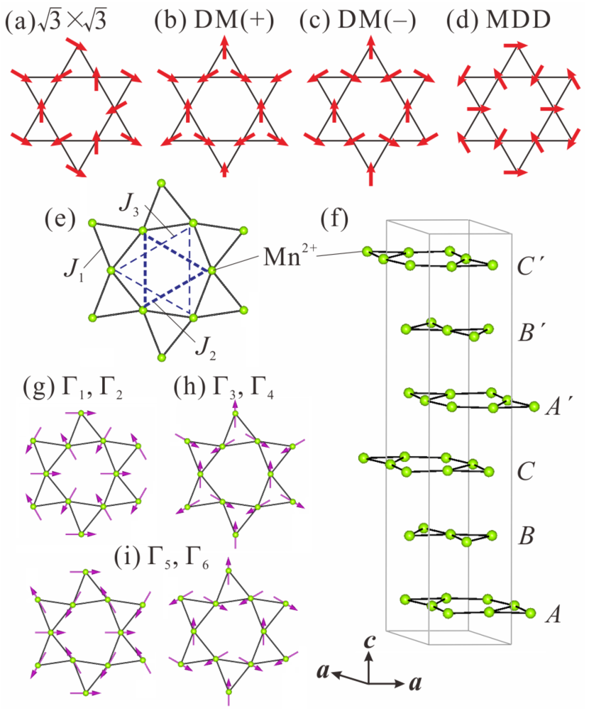
Figure 1: 120^∘ structures in the Kagome lattice. The directions of the spins are represented by the red arrows. (a) 120^∘ structure with the enlarged unit cell by $\sqrt{3}\times\sqrt{3}$. (b) DM(+), (c) DM($-$), and (d) MDD-type 120^∘ structure with the propagation vector $\bm{k}=0$. (e) Mn²⁺ ions in a Kagome layer in NaBa₂Mn₃F₁₁. Solid, thick-dashed and thin-dashed lines indicate the nearest-, second-, and third-neighbor interactions. The lattice is equivalent to the regular Kagome lattice as a spin system (see text). (f) The linear perspective view of the Kagome layers. (g)-(i) 120^∘ structures represented by the IRs for $\bm{k}=0$.

In a classical Heisenberg Kagome antiferromagnet, the ground state is infinitely degenerated. At zero temperature long-range order of the 120^∘ structures with enlarged $\sqrt{3}\times\sqrt{3}$ unit cells characterized by ${\bm{k}}_{1/3}=(1/3,1/3,0)$ in Fig. 1(a) is selected by the order-by-disorder mechanism PRB48 . The degeneracy of the ground state can be lifted also by various perturbations. The states selected by the Dzyaloshinskii-Moriya (DM) interaction are the 120^∘ structures with $\bm{k}_{0}=(0,0,0)$ PRB66 ; the structures exhibit positive vector chirality in Fig. 1(b) and negative vector chirality in Fig. 1(c). We name DM($+$)- and DM($-$)-type 120^∘ structures for the former and the latter, respectively. The vector chirality is determined by the out-of-plane component of the DM vector. In the DM($+$) structure, the easy-axis anisotropy is induced by the in-plane component of the DM vector. The state selected by the MDD interaction is the 120^∘ structure exhibiting tail-chase geometry as shown in Fig. 1(d) PRB91 . It has positive chirality but different easy-axis anisotropy from the DM($+$) structure. It is named the MDD-type 120^∘ structure. The structure is equivalent to magnetic vortices on a honeycomb lattice with staggered polarity, which can be a prototype of a natural magnonic crystal Sugimoto11 ; Jain12 ; Hanze16 . The states selected by the second-neighbor interaction are the 120^∘ structure with $\bm{k}_{0}$ for the antiferromagnetic case and that with $\bm{k}_{1/3}$ for the ferromagnetic case PRB72_J2 .

The magnetic structures of the Kagome antiferromagnet have been intensively investigated by neutron diffraction on many compounds. The DM($+$) structure is realized in most cases; $A$Fe₃(SO₄)₂(OH)₆ ($A=$ K, Na, Ag, Rb, NH₄) PRB61 ; PRB63 ; PRB61_DMp ; PRB67_DMp , KCr₃(SO₄)₂(OH)₆ PRB64 , and Nd₃Sb₃Mg₂O₁₄ PRB93 , which may be due to the coincidence between the direction of spins determined by DM interaction and the magnetic easy axis allowed by the crystallographic symmetry. The DM($-$) structure is observed in a couple of semimetals Mn₃Sn and Mn₃Ge exhibiting large anomalous Hall effect SSC42_DMm . The $\sqrt{3}\times\sqrt{3}$ structure is found in the high pressure phase in herbertsmithite ZnCu₃(OH)₆Cl₂ PRL108_sqrt3 . The tail-chase structure was observed in quinternary oxalate compounds with Fe²⁺ ion PRL107_MDD ; EPJB_MDD so far. Its tail-chase structure was, however, caused by a strong single-ion anisotropy instead of the MDD interaction. To the best of our knowledge, the experimental observation of the tail-chase structure originating from the MDD interaction has not yet been identified (by neutron diffraction) although it is of primary importance to the understanding of the Kagome family of compounds.

NaBa₂Mn₃F₁₁ crystallizes in a hexagonal structure with the space group $R\bar{3}c$ JSSC98 . Mn²⁺ ions carry spin $S=5/2$, and MnF₇ pentagonal bipyramids form a Kagome lattice in the crystallographic $ab$-plane as shown in Fig. 1(e). The path of the nearest-neighbor interaction $J_{1}$ indicated by the solid line is Mn-F-Mn. Although the interior angles of the hexagon in the Kagome lattice are shifted from 120^∘ and the lattice is distorted, the length of the sides and the angles of Mn-F-Mn are the same for all the bonds. This means that the magnitudes of the nearest-neighbor interactions are the same. The spin system is thus regarded as the regular Kagome lattice. The six Kagome layers are stacked in the unit cell as shown in Fig. 1(f). The $A$, $B$, and $C$ layers and $A^{\prime}$, $B^{\prime}$, and $C^{\prime}$ layers are related by the $c$-glide.

The exchange pathways of the second and third-neighbor interaction are unusual; the second-neighbor interaction $J_{2}$ indicated by the thick dashed line is Mn-F-Mn, and that of the third-neighbor interaction $J_{3}$ indicated by the thin dashed line is Mn-F-F-Mn. The $J_{3}$ is thus negligible, and the unique network called Kagome-Triangular lattice is realized JPSJ83 . The heat capacity and magnetic susceptibility measurements exhibit antiferromagnetic transition at $T_{{\rm N}}=2$ K. The Curie-Weiss temperature $\theta_{{\rm CW}}$ was estimated to be $-32$ K, which is smaller than those of most Kagome lattice magnets PRB61 ; PRB63 ; PRB61_DMp ; PRB67_DMp ; PRB64 ; PRB93 ; PRL108_sqrt3 . In addition, the bond angles of the nearest neighbor exchange pathways are close to 90^∘ rather than 180^∘ JPSJ83 , suggesting the nearest neighbor interaction is weak antiferromagnet or ferromagnetic based on the Goodenough-Kanamori rules goodenough ; kanamori . The exchange interaction in NaBa₂Mn₃F₁₁ is thus relatively small, and the MDD interaction may be important.

In this paper, we demonstrate that the tail-chase structure with small incommensurate (IC) modulations is realized in NaBa₂Mn₃F₁₁ by using neutron diffraction. Combination of the experiment and calculation suggests that the tail-chase structure selected by the main perturbation of the short-range MDD interaction including up to the fourth neighboring is modulated by a smaller perturbation such as the long-range MDD interaction or the interlayer interaction.

II Experimental details

A polycrystalline sample was prepared by a solid state reaction method JPSJ83 . The total mass of the obtained sample was 5.4 g. A ³He cryostat was used to achieve low temperatures. Neutron diffraction experiments were performed using two neutron diffractometers; a powder diffractometer ECHIDNA installed in OPAL reactor, Australian Nuclear Science and Technology Organization for the preliminary measurement, and a long-wavelength time-of-flight (TOF) diffractometer WISH wish installed at the ISIS Pulsed Neutron and Muon Source, Rutherford Appleton Laboratory for the precise measurement. We chose a high resolution double frame mode at WISH. The data for the Rietveld refinement in Figs. 2(a), 2(b) and the temperature dependence of the integrated intensities in Fig. 3(a) were measured by using the detector bank with an average scattering angle of $2\theta=90^{\circ}$. The data for the diffuse scattering in Fig. 3(b) were measured by using the detector bank centered at $2\theta=27^{\circ}$. The obtained data were analyzed by the Rietveld method using FullProf software PhysicaB192 . Candidates for the magnetic structure compatible with the lattice symmetry were obtained by the SARA$h$ software PhysicaB276 .

III Results and analysis

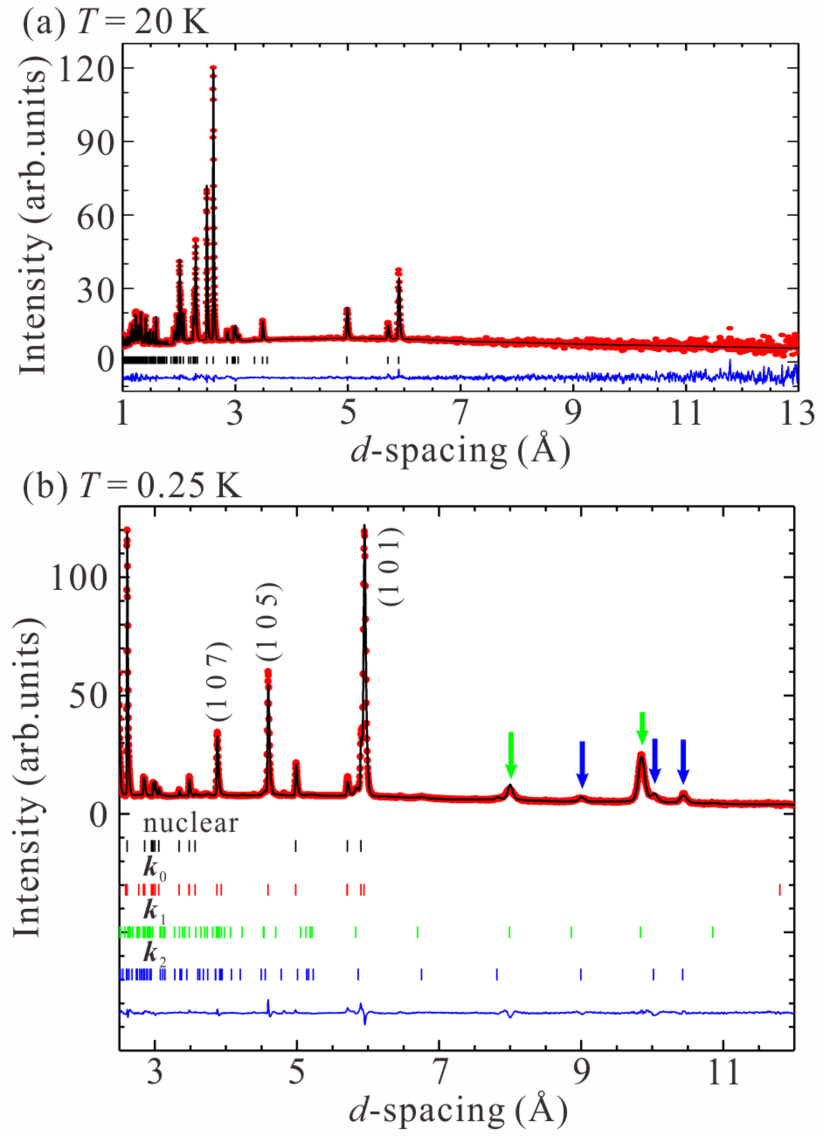
Figure 2: Neutron diffraction profiles for NaBa₂Mn₃F₁₁ at (a) 20 K and (b) 0.25 K. The solid squares and curves show the experimental data and simulations, respectively. The vertical bars show the positions of the nuclear and magnetic Bragg peaks. The solid curves below the bars show the difference between the data and simulations. The green and blue arrows indicate the IC magnetic Bragg peaks with $\bm{k}_{1}$ and $\bm{k}_{2}$.

The neutron diffraction profile measured at 20 K is reasonably fitted by the hexagonal structure with the space group $R\overline{3}c$ as shown in Fig. 2(a). The profile factors are $R_{{\rm wp}}=8.80\%$ and $R_{{\rm e}}=4.37\%$, and the obtained parameters are summarized in the cif file in supplemental information.

At 0.25 K, at least eight additional peaks are observed as shown in Fig. 2(b). The peak intensities increase with the decrease of the temperature below 2.25 K as shown in Fig. 3(a). This means that a magnetic long range order occurs at $T_{\rm N}=2.25$ K, which is consistent with the previous heat capacity measurement JPSJ83 . The peaks at $d=$ 3.8, 4.6, and 5.9 Å are indexed as (1 0 7), (1 0 5), and (1 0 1), meaning that the magnetic propagation vector is $\bm{k}_{0}=(0,0,0)$. The peaks indicated by the green and blue arrows in the long $d$ region are not indexed by the $\bm{k}_{0}$ but by IC vectors.

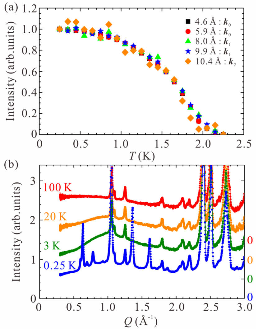
Figure 3: (a) Temperature evolution of the integrated intensities at $d=$ 4.6, 5.9, 8.0, 9.9 and 10.4 Å. The error bars are inside the markers. Each of integrated intensities is normalized to their values at 0.25 K and subtracted by their background at 2.25 K. (b) Neutron diffraction profiles at $T=$ 100, 20, 3 and 0.25 K. The profiles are shifted by vertical offsets.

Temperature variation of the diffraction profiles are exhibited in Fig. 3(b). At 100 K paramagnetic scattering is observed in the low $Q$ region. On cooling it is suppressed, and, instead, magnetic diffuse scattering is induced at $Q\sim$ 1.0 Å^-1 and more pronounced at 3 K. The diffuse scattering is suppressed with further cooling, and magnetic Bragg peaks appear. The short-range spin correlations thus develop at much higher temperature than the transition temperature, suggesting the existence of strong geometrical frustration. The behavior is consistent with the heat capacity in which most of the magnetic entropy was released above $T_{{\rm N}}$ JPSJ83 .

In the magnetic structure analysis, it is assumed that the peaks with $\bm{k}_{0}$ mainly construct the magnetic structure, since the intensities of the peaks with $\bm{k}_{0}$ are larger than those with the IC vectors. The representation analysis PhysicaB276 with the space group $R\bar{3}c$ and the propagation vector $\bm{k}_{0}$ leads to six irreducible representations (IRs) $\Gamma_{1}+\Gamma_{2}+\Gamma_{3}+\Gamma_{4}+2\Gamma_{5}+2\Gamma_{6}$. The IRs and the basis vectors are summarized in Table 1. The basis vectors for $\Gamma_{1}$ or $\Gamma_{2}$ provide the MDD-type 120^∘ structure in Fig. 1(g), and $\Gamma_{3}$ or $\Gamma_{4}$ provide the DM($+$)-type structure in Fig. 1(h) whereas the basis vectors associated with $\Gamma_{5}$ or $\Gamma_{6}$ correspond to the 120^∘ structure with the negative vector chirality as shown in Fig. 1(i). The magnetic structure in the ${\alpha}$ layer (${\alpha}=A,B,C$) and that in the ${\alpha}^{\prime}$ layer (${\alpha}^{\prime}=A^{\prime},B^{\prime},C^{\prime}$) are the same for $\Gamma_{1}$, $\Gamma_{3}$ and $\Gamma_{5}$. In contrast, the structure in the ${\alpha}^{\prime}$ layer is the inversed structure of the ${\alpha}$ layer for $\Gamma_{2}$, $\Gamma_{4}$, and $\Gamma_{6}$. In testing the models of the magnetic structures inferred by the various IRs, it is assumed that the magnitude of the magnetic moments on the Mn²⁺ ions are all the same. From the Rietveld refinements, we find that only $\Gamma_{2}$ gives a satisfactory agreement with the observed pattern. The refined magnetic structure with $\bm{k}_{0}$ exhibits the 120^∘ structure in the $ab$-plane as shown in Fig. 1(g). The refined magnitude of the moment is 4.14(1) $\mu_{{\rm B}}$ at 0.25 K, which is 83$\%$ of the full moment of Mn²⁺ ion. According to the $J_{1}$ - $J_{2}$ phase diagram in the Heisenberg Kagome-Triangular lattice JPSJ83 , the 120^∘ structure with $\bm{k}_{0}$ is favored in case that both of $J_{1}$ and $J_{2}$ are antiferromagnetic. This means that both of $J_{1}$ and $J_{2}$ in this compound are antiferromagnetic in the absence of MDD interaction.

We search the propagation vectors of the IC peaks corresponding high symmetry points/lines/planes of the Brillouin Zone. The IC peaks are indexed by two propagation vectors: $\bm{k}_{1}=(0.3209(2),0.3209(2),0)$ for the peaks at $d=$ 8.0 and 9.9 Å and $\bm{k}_{2}=(0.3338(4),0.3338(4),0)$ for those at $d=$ 9.0, 10.0 and 10.4 Å. The IC vectors are close to ${\bm{k}}_{1/3}=(1/3,1/3,0).$ The representation analysis with the space group $R\bar{3}c$ and the propagation vectors $\bm{k}_{1}$ and $\bm{k}_{2}$ leads to separation of the equivalent Mn sites into the four nonequivalent Mn sites, and two IRs $\Gamma_{1}+\Gamma_{2}$ at each of the four Mn sites. The IRs and the basis vectors are summarized in Table 2. We construct the models of the magnetic structure by the linear combinations of the basis vectors in each single IR. The explicit formulas of the magnetic models that are compatible with both propagation vectors and the space group in the case of $\Gamma_{2}$ are as follow:

$$\bm{m}_{{\rm Mn1a}} = c_{4}^{(1)}\Psi_{4}^{(1)}+c_{5}^{(1)}\Psi_{5}^{(1)}+c_{6}^{(1)}\Psi_{6}^{(1)},$$ (1)

$$\bm{m}_{{\rm Mn1b}} = c_{4}^{(1)}\Psi_{4}^{(1)}+c_{5}^{(1)}\Psi_{5}^{(1)}+c_{6}^{(1)}\Psi_{6}^{(1)},$$ (2)

$$\bm{m}_{{\rm Mn2}} = c_{2}^{(2)}\Psi_{2}^{(2)}+c_{3}^{(2)}\Psi_{3}^{(2)},$$ (3)

$$\bm{m}_{{\rm Mn3a}} = (c_{4^{\prime}}^{(1)}\Psi_{4}^{(3)}+c_{5^{\prime}}^{(1)}\Psi_{5}^{(3)})+c_{6^{\prime}}^{(1)}\Psi_{6}^{(3)},$$ (4)

$$\bm{m}_{{\rm Mn3b}} = (c_{4^{\prime}}^{(1)}\Psi_{4}^{(3)}+c_{5^{\prime}}^{(1)}\Psi_{5}^{(3)})+c_{6^{\prime}}^{(1)}\Psi_{6}^{(3)},$$ (5)

$$\bm{m}_{{\rm Mn4}} = c_{2^{\prime}}^{(2)}\Psi_{2}^{(4)}+c_{3^{\prime}}^{(2)}\Psi_{3}^{(4)}.$$ (6)

Here the coordinations of the Mn atoms and the basis vectors $\Psi_{i}^{(j)}$ are exhibited in Table 2. $c_{4}^{(1)}$, $c_{5}^{(1)}$, $c_{6}^{(1)}$, $c_{4^{\prime}}^{(1)}$, $c_{5^{\prime}}^{(1)}$, $c_{6^{\prime}}^{(1)}$, $c_{2}^{(2)}$, $c_{3}^{(2)}$, $c_{2^{\prime}}^{(2)}$ and $c_{3^{\prime}}^{(2)}$ are coefficients of the linear combination of the basis vectors. The number of the fitting parameters is 10, which is too many for the number of the observed IC peaks. We therefore assumed that the magnetic structures in the six layers are as similar as possible, and the formulas used for the refinement were reduced to:

$$\bm{m}_{{\rm Mn1a}} = c_{4}^{(1)}\Psi_{4}^{(1)}+c_{5}^{(1)}\Psi_{5}^{(1)}+c_{6}^{(1)}\Psi_{6}^{(1)},$$ (7)

$$\bm{m}_{{\rm Mn1b}} = c_{4}^{(1)}\Psi_{4}^{(1)}+c_{5}^{(1)}\Psi_{5}^{(1)}+c_{6}^{(1)}\Psi_{6}^{(1)},$$ (8)

$$\bm{m}_{{\rm Mn2}} = c_{2}^{(2)}\Psi_{2}^{(2)}+c_{3}^{(2)}\Psi_{3}^{(2)},$$ (9)

$$\bm{m}_{{\rm Mn3a}} = t_{1}(c_{4}^{(1)}\Psi_{4}^{(3)}+c_{5}^{(1)}\Psi_{5}^{(3)})+t_{2}c_{6}^{(1)}\Psi_{6}^{(3)},$$ (10)

$$\bm{m}_{{\rm Mn3b}} = t_{1}(c_{4}^{(1)}\Psi_{4}^{(3)}+c_{5}^{(1)}\Psi_{5}^{(3)})+t_{2}c_{6}^{(1)}\Psi_{6}^{(3)},$$ (11)

$$\bm{m}_{{\rm Mn4}} = t_{1}c_{2}^{(2)}\Psi_{2}^{(4)}+t_{2}c_{3}^{(2)}\Psi_{3}^{(4)}.$$ (12)

$t_{1}$ and $t_{2}$ take $+1$ or $-1$. This reduces the number of parameters down to 5 and renders the refinement possible. We similarly construct the magnetic models in the case of $\Gamma_{1}$. The best fit is obtained for the $\Gamma_{2}$, and the parameters are listed in Table 3. The profiles at 0.25 K and fitting results of the model combining with $\bm{k}_{0}$, $\bm{k}_{1}$, and $\bm{k}_{2}$ are shown in Fig. 2(b). The $R$ factors for the whole profile are $R_{{\rm wp}}=7.61\%$ and $R_{{\rm e}}=1.02\%$. The magnetic $R$ factors $R_{{\rm mag}}$ for $\bm{k}_{0}$, $\bm{k}_{1}$, and $\bm{k}_{2}$ are $2.71\%$, $7.62\%$, and $12.8\%$. For the reference, the best $R_{{\rm mag}}$s for $\bm{k}_{0}$ are $57\%$ for $\Gamma_{1}$, $89\%$ for $\Gamma_{3}$, $80\%$ for $\Gamma_{4}$, $79\%$ for $\Gamma_{5}$, and $36\%$ for $\Gamma_{6}$. The refined magnetic moments in each IC structure with $\bm{k}_{1}$ and $\bm{k}_{2}$ form the two-in-one-out (one-in-two-out) structure similar to the Kagome spin ice PRB66_wills . In addition, they have an out of plane component, the directions of which are all up or all down, and the magnitudes of the moments are modulated.

The temperature evolutions of the integrated intensities associated with the propagation vectors $\bm{k}_{0}$, $\bm{k}_{1}$, and $\bm{k}_{2}$ are the same as shown in Fig. 3(a). This suggests that the low temperature state is a single ordered state, i.e., a multiple-$\bm{k}$ state, where the Mn²⁺ moments form a 120^∘ structure in the $ab$-plane, and the IC propagation vectors modulate this 120^∘ structure. The averaged magnitude of the magnetic moment of the Mn²⁺ ion is 4.54 $\mu_{{\rm B}}$ at 0.25 K, which is 91$\%$ of the Mn²⁺ moment $(S=5/2)$.

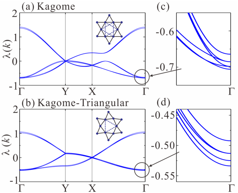
Figure 4: Eigenvalues of the interaction matrix $J_{ij}^{\alpha\beta}$ along lines in the Brillouin zone. Spectra in (a) the Kagome lattice and (b) the Kagome-Triangular lattice where the exchange interactions are $J_{1}=J_{2}=2$ K and the MDD interaction is $J_{{\rm MDD}}=56$ mK. (c), (d) Detailed structures of the spectra around the $\Gamma$ point.

IV Discussion

For the calculation of the ground state we assume isotropic Heisenberg interactions, since the orbital angular momentum of Mn²⁺ ion is zero, at least for the ground state of the isolated Mn²⁺ ion, and the anisotropy and/or asymmetric terms derived from the perturbation of spin-orbit coupling should be small. As described in the introduction section, the geometry of the main framework of NaBa₂Mn₃F₁₁ is a Kagome-Triangular lattice and MDD interaction is not negligible. The following Hamiltonian in a Kagome plane is thus a good approximation for this system:

$${\mathcal{H}} =\sum_{{\rm n.n.}}J_{1}\bm{S}_{i}\cdot\bm{S}_{j}+\sum_{{\rm n.n.n.}}J_{2}\bm{S}_{i}\cdot\bm{S}_{j}$$

$$+ \sum_{i,j}\frac{\mu_{0}}{4\pi}\frac{(g\mu_{{\rm B}})^{2}}{|\bm{r}_{ij}|^{3}}\left[\bm{S}_{i}\cdot\bm{S}_{j}-3\frac{\left(\bm{S}_{i}\cdot\bm{r}_{ij}\right)\left(\bm{S}_{j}\cdot\bm{r}_{ij}\right)}{|\bm{r}_{ij}|^{2}}\right],$$

where $J_{1}$ and $J_{2}$ are the exchange interactions in the nearest- and second-neighbor paths. The third term is the MDD interaction up to the fourth-neighbor paths and $\bm{r}_{ij}$ is the bond vector between the spins. The strength of the nearest neighbor MDD interaction $J_{{\rm MDD}}$ is 56 mK, which is determined from the distance of the nearest neighbor path $r_{{\rm n.n.}}$as follow:

$$J_{{\rm MDD}}\equiv\frac{\mu_{0}}{4\pi}\frac{(g\mu_{{\rm B}})^{2}}{r_{{\rm n.n.}}^{3}}=56~{}{\rm mK}.$$ (14)

In the calculation, the interlayer interaction is not included. To calculate the ground state of the system, we use a Luttinger-Tisza-type theory PR70 , and investigate the eigenenergies and eigenvectors of the interaction matrix in the wave vector space. The Fourier transformed Hamiltonian can be written as

$${\mathcal{H}}=\sum_{\bm{k}}\sum_{i,j}\sum_{\alpha,\beta}J_{ij}^{\alpha\beta}(\bm{k})S_{i}^{\alpha}(-\bm{k})S_{j}^{\beta}(\bm{k}),$$ (15)

where $J_{ij}^{\alpha\beta}$ is the sum of $J_{1}$, $J_{2}$, and $J_{{\rm MDD}}$. Here, $\alpha$ and $\beta$ are the Cartesian indices of the spins and $i$, $j$ run over the three basis sites in the unit cell of the Kagome lattice. The spin vector is the Fourier component of the real space, and $\bm{k}$ runs over the Brillouin zone of the Kagome lattice. Thus, for a given value of $\bm{k}$, $J_{ij}^{\alpha\beta}$ is a $9\times 9$ matrix that needs to be diagonalized. We calculate for two cases: Kagome lattice with second-neighbor interaction in Fig. 4(a) and Kagome-Triangular lattice in Fig. 4(b). $(0,0,0)$, $(1/3,1/3,0)$, and $(1/2,0,0)$ points of the Brillouin zone are labeled as the $\Gamma$, X, and Y, respectively. In order to realize the 120^∘ structure with $\bm{k}=0$, we set antiferromagnetic interactions for both $J_{1}$ and $J_{2}$ PRB72_J2 ; JPSJ83 . Since varying $J_{2}/J_{1}$ does not make a significant difference to the results within a wide range of values, the exchange interactions are parametrized at $J_{1}=J_{2}$ for simplicity. We also put $J_{1}>J_{{\rm MDD}}$ because the Curie-Weiss temperature $\theta_{{\rm CW}}=-32$ K JPSJ83 is larger than the $J_{{\rm MDD}}=56$ mK.

The eigenenergy $\lambda(\bm{k})$ is minimized for $\bm{k}=0$ in both lattices as shown in Figs. 4(a) and 4(b) which implies that the MDD-type 120^∘ structures in Fig. 1(d) is realized for both Kagome and Kagome-Triangular lattices. This result is consistent with the previous study PRB91 . Although the six states are degenerated at $\bm{k}=0$ in the absence of MDD interaction, the degeneracy is lifted by the interaction as shown in Figs. 4(c) and 4(d). The calculated ground states correspond to the magnetic structure having $\bm{k}_{0}$ in the experiment, but they do not reproduce the multiple-$\bm{k}$ structure.

For the multiple-$\bm{k}$ structure, we calculated the ground state of the Kagome-Triangular antiferromagnet including $J_{3}$ interaction in Fig. 1(e). The obtained phase diagram of $J_{3}/J_{1}$ - $J_{2}/J_{1}$, where $J_{1}$ is antiferromagnetic, is shown in Fig. 5(a). We have presumed that $J_{1}\sim J_{2}\gg|J_{3}|$ so far, and the observed $\bm{k}_{0}$ structure is confirmed by the calculation in this region. In case that $J_{2}$ and $J_{3}$ are ferromagnetic, i.e., in the third quadrant, the state of $\bm{k}_{1/3}=(1/3,1/3,0)$ which is close to the experimentally observed IC vectors $\bm{k}_{1}$ and $\bm{k}_{2}$ appears. The ground energy has, however, a single minimum in the $\bm{k}$ space, and the observed a multiple-$\bm{k}$ structure cannot be explained. Then the MDD interaction up to the 4th-neighbor paths is included, and the eigenvalues of the interaction matrix for $J_{1}$ = 2 K, $J_{2}$ = $J_{3}$ = $-J_{\rm MDD}/2$ is obtained as shown in Figs. 5(b) and 5(c). Local minima appear at $\bm{k}=(1/3,1/3,0)$ and $(0,0,0)$, indicating the multiple-$\bm{k}$ structure. We found that the MDD interaction mixes the $\bm{k}_{0}$ structure in the first quadrant and $\bm{k}_{1/3}$ structure in the third quadrant in the $J_{3}/J_{1}$ - $J_{2}/J_{1}$ phase diagram. The spin structure for $\bm{k}_{0}$ is the tail-chase structure which is consistent with the experiment. The one for $\bm{k}_{1/3}$ has solely out-of-plane component, and it exhibits up-up-down structure. This is inconsistent with the experimentally obtained structure. We have surveyed a series of parameters and exact match to the experimental structure could not be found. Thus, the terms in Eq. (LABEL:hamiltonian) do not explain the observed multiple-$\bm{k}$ structure, and neither does $J_{3}$. Detailed theoretical studies considering further interactions including the long-range MDD interaction and/or the interlayer interaction are necessary to reproduce the observed multiple-$\bm{k}$ structure including IC modulation for the future work.

Figure 5: (a) Phase diagram of Kagome-Triangular antiferromagnet having $J_{3}$ interaction. MDD interaction is not included. (b), (c) Eigenvalues of the interaction matrix $J_{ij}^{\alpha\beta}$ for Kagome-Triangular antiferromagnet having $J_{3}$ and MDD interaction along lines in the Brillouin zone, where the parameters are $J_{1}$ = 2 K and $J_{2}=J_{3}=-J_{\rm MDD}/2$. The panel (b) is for wide energy range and the panel (c) is for low energy range. Double minima structure is observed.

The reason why the MDD interaction is the main perturbation in NaBa₂Mn₃F₁₁ is due to the fact that the exchange interaction is weak compared with most of Kagome antiferromagnets having O^2- as anion that transfers the exchange integral PRB61 ; PRB63 ; PRB61_DMp ; PRB67_DMp ; PRB64 ; PRB93 . Hybridization of the $d$ and $p$ orbitals is small in fluorides compared with oxides since covalency of F^- ion is weaker than that of O^2- ion. In addition, the edge-sharing of the pentagonal bipyramids MnF₇ in the nearest neighbor path weakens the antiferromagnetic exchange interaction. The superexchange interaction is thus weak and, consequently, DM interaction, that is resulting term of the perturbative treatment of the exchange interaction and spin-orbit interaction in the Heisenberg spin Hamiltonian, is also weak. Furthermore, the charge distribution of Mn²⁺ ion is spherical and prevents the appearance of single-ion anisotropy, since the $3d$ orbitals are half filled, with five electrons coupled giving rise to an angular momentum $L=0$. The MDD interaction hence causes the main perturbation in NaBa₂Mn₃F₁₁.

V Conclusion

In conclusion the MDD-type 120^∘ structure with an IC modulation was identified in NaBa₂Mn₃F₁₁ by the combination of the neutron diffraction measurement and magnetic structure analysis. Classical calculations showed that the MDD interaction is the main perturbative term for the selection of the magnetic ground state. To elucidate the precise IC structure and to identify its origin, further investigations, for instance single crystal neutron diffraction, are required. Theoretical calculation including long-range MDD interactions may elucidate the IC structure, as was the case with the field-induced IC structure in the gadolinium gallium garnet PRL97_GGG ; PRL114_GGG . Consideration on the interlayer interaction would be also important. In addition, the study on magnetic dynamics would be beneficial for the search of exotic states induced by the MDD interaction.

References

- (1) J. Stuhler, A. Griesmaier, T. Koch, M. Fattori, T. Pfau, S. Giovanazzi, P. Pedri, and L. Santos, Phys. Rev. Lett. 95, 150406 (2005).
- (2) H. M. Rønnow, R. Parthasarathy, J. Jensen, G. Aeppli, T. F. Rosenbaun, and D. F. McMorrow, Science 308, 389 (2005).
- (3) C. Kraemer, N. Nikseresht, J. O. Piatak, N. Tsyrulin, B. D. Piazza, K. Kiefer, B. Klemke, T. F. Rosenbaum, G. Aeppli, C. Gannarelli, K. Prokes, A. Podlesnyak, T. Strässle, L. Keller, O. Zaharko, K. W. Krämer, and H. M. Rønnow, Science 336, 1416 (2012).
- (4) E. Burzurí, F. Luis, B. Barbara, R. Ballou, E. Ressouche, O. Montero, J. Campo, and S. Maegawa, Phys. Rev. Lett. 107, 097203 (2011).
- (5) S. Sugimoto, Y. Fukuma, S. Kasai, T. Kimura, A. Barman, and Y. C. Otani, Phys. Rev. Lett. 106, 197203 (2011).
- (6) S. Jain, V. Novosad, F. Y. Fradin, J. E. Pearson, V. Tiberkevich, A. N. Slavin, and S. D. Bader, Nat. Commun. 3, 1330 (2012).
- (7) M. Hänze, C. F. Adolff, B. Schulte, J. Möller, M. Weigand, and G. Meier, Sci. Rep. 6, 22402 (2016).
- (8) J. M. Luttinger and L. Tisza, Phys. Rev. 70, 954 (1946).
- (9) W. L. Roth, Phys. Rev. 110, 1333 (1958).
- (10) A. Schrön, C. Rödl, and F. Bechstedt, Phys. Rev. B 86, 115134 (2012).
- (11) D. C. Johnston, Phys. Rev. B 93, 014421 (2016).
- (12) J. S. Gardner, M. J. P. Gingras, and J. E. Greedan, Rev. Mod. Phys. 82, 53 (2010).
- (13) C. Nisoli, R. Moessner, and P. Schiffer, Rev. Mod. Phys. 85, 1473 (2013).
- (14) J. N. Reimers and A. J. Berlinsky, Phys. Rev. B 48, 9539 (1993).
- (15) M. Elhajal, B. Canals and C. Lacroix, Phys. Rev. B 66, 014422 (2002)
- (16) M. Maksymenko, V. R. Chandra, and R. Moessner, Phys. Rev. B 91, 184407 (2015).
- (17) J.-C. Domenge, P. Sindzingre, C. Lhuillier, and L. Pierre, Phys. Rev. B 72, 024433 (2005).
- (18) T. Inami, M. Nishiyama, S. Maegawa, and Y. Oka, Phys. Rev. B 61, 12181 (2000).
- (19) A. S. Wills, Phys. Rev. B 63, 064430 (2001).
- (20) A. S. Wills, A. Harrison, C. Ritter, and R. I. Smith, Phys. Rev. B 61, 6156 (2000).
- (21) D. Grohol, D. G. Nocera, and D. Papoutsakis, Phys. Rev. B 67, 064401 (2003).
- (22) T. Inami, T. Morimoto, M. Nishiyama, S. Maegawa, Y. Oka, and H. Okumura, Phys. Rev. B 64, 054421 (2001).
- (23) A. Scheie, M. Sanders, J. Krizan, Y. Qiu, R. J. Cava, and C. Broholm, Phys. Rev. B 93, 180407(R) (2016).
- (24) T. Nagamiya, S. Tomiyoshi, and Y. Yamaguchi, Solid State Commun. 42, 385 (1982)
- (25) D. P. Kozlenko, A. F. Kusmartseva, E. V. Lukin, D. A. Keen, W. G. Marshall, M. A. de Vries, and K. V. Kamenev, Phys. Rev. Lett. 108, 187207 (2012).
- (26) E. Lhotel, V. Simonet, J. Ortloff, B. Canals, C. Paulsen, E. Suard, T. Hansen, D. J. Price, P. T. Wood, A. K. Powell, and R. Ballou, Phys. Rev. Lett. 107, 257205 (2011).
- (27) E. Lhotel, V. Simonet, J. Ortloff, B. Canals, C. Paulsen, E. Suard, T. Hansen, D. J. Price, P. T. Wood, A. K. Powell, and R. Ballon, Eur. Phys. J. B 86, 248 (2013).
- (28) J. Darriet, M. Ducau, M. Feist, A. Tressaud, and P. Hagenmuller, J. Solid State Chem. 98, 379 (1992).
- (29) H. Ishikawa, T. Okubo, Y. Okamoto and Z. Hiroi, J. Phys. Soc. Jpn. 83, 043703 (2014).
- (30) J. B. Goodenough, Phys. Rev. 100, 564 (1955).
- (31) J. Kanamori, J. Phys. Chem. Solids 10, 87 (1959).
- (32) L. C. Chapon, P. Manuel, P. G. Radaelli, C. Benson, L. Perrott, A. Ansell, N. J. Rhodes, D Raspino, D. Duxbury, E. Spill, and J. Norris, Neutron News 22, 22 (2011).
- (33) J. Rodriguez-Carvajal, Physica B 192, 55 (1993).
- (34) A. S. Wills, Physica B 276-278, 680 (2000).
- (35) A. S. Wills, R. Ballou, and C. Lacroix, Phys. Rev. B 66, 144407 (2002).
- (36) T. Yavors’kii, M. Enjalran, and M. J. P. Gingras, Phys. Rev. Lett. 97, 267203 (2006).
- (37) N. d’Ambrumenil, O. A. Petrenko, H. Mutka, and P. P. Deen, Phys. Rev. Lett. 114, 227203 (2015).