The Ultra-Fast Outflow of the Quasar PG 1211+143
as Viewed by Time-Averaged Chandra Grating Spectroscopy

Abstract

We present a detailed X-ray spectral study of the quasar PG 1211+143 based on Chandra High Energy Transmission Grating Spectrometer (HETGS) observations collected in a multi-wavelength campaign with UV data using the Hubble Space Telescope Cosmic Origins Spectrograph (HST-COS) and radio bands using the Jansky Very Large Array (VLA). We constructed a multi-wavelength ionizing spectral energy distribution using these observations and archival infrared data to create xstar photoionization models specific to the PG 1211+143 flux behavior during the epoch of our observations. Our analysis of the Chandra-HETGS spectra yields complex absorption lines from H-like and He-like ions of Ne, Mg and Si which confirm the presence of an ultra-fast outflow (UFO) with a velocity $\sim-$17 300 km s^-1 (outflow redshift $z_{\rm out}\sim-0.0561$) in the rest frame of PG 1211+143. This absorber is well described by an ionization parameter $\log\xi\sim 2.9$ erg s^-1 cm and column density $\log N_{\rm H}\sim 21.5$ cm^-2. This corresponds to a stable region of the absorber’s thermal stability curve, and furthermore its implied neutral hydrogen column is broadly consistent with a broad Ly$\alpha$ absorption line at a mean outflow velocity of $\sim-16\,980$ km s^-1 detected by our HST-COS observations. Our findings represent the first simultaneous detection of a UFO in both X-ray and UV observations. Our VLA observations provide evidence for an active jet in PG 1211+143, which may be connected to the X-ray and UV outflows; this possibility can be evaluated using very-long-baseline interferometric observations.

]Received 2017 October 17; revised 2017 December 14; accepted 2017 December 18; published 2018 February 2

1. Introduction

X-ray observations of active galactic nuclei (AGNs) reveal blueshifted absorption features, which have been interpreted as outflows of photoionized gas along the line of sight (Halpern, 1984). Soft X-ray absorption lines are commonly referred to as warm absorbers (WAs), while those ionized absorbers with a velocity higher than 10 000 km s^-1 are defined as ultra-fast outflows (UFOs; Tombesi et al., 2010). WAs have been observed in over half of Seyfert 1 galaxies (e.g., Reynolds & Fabian, 1995; Reynolds, 1997; George et al., 1998; Laha et al., 2014), which exhibit outflow velocities in the range of 100–500 km s^-1 (e.g., Kaspi et al., 2000; Blustin et al., 2002; McKernan et al., 2007). On the other hand, X-ray observations of iron absorption lines can indicate outflow velocities that are quite large, up to mildly relativistic values of $\sim 0.1$–$0.4c$ (e.g., Pounds et al., 2003; Cappi, 2006; Braito et al., 2007; Cappi et al., 2009). More recent studies show that UFOs are identified in a significant fraction ($\sim 30$ per cent) of radio-quiet and radio-loud AGNs (Tombesi et al., 2010, 2011, 2012, 2014). Recently, Tombesi et al. (2013) concluded that UFOs and WAs are associated with different locations of a single large-scale stratified outflow in the AGN, suggesting a unified model for accretion powered sources (Kazanas et al., 2012). However, Laha et al. (2014, 2016) instead suggested that UFOs and WAs may be associated with two different outflows with distinctive physical conditions and outflow velocities.

Table 1Observation log of PG 1211+143

Observatory	Detector	Gratings	Seq./PID	Obs.ID	UT Start	UT End	Time (ks)
Chandra	ACIS-S	HETGS	703109	17109	2015 Apr 09, 08:22	2015 Apr 10, 14:32	104.68
Chandra	ACIS-S	HETGS	703109	17645	2015 Apr 10, 17:55	2015 Apr 11, 06:56	44.33
Chandra	ACIS-S	HETGS	703109	17646	2015 Apr 12, 02:04	2015 Apr 13, 02:15	83.65
Chandra	ACIS-S	HETGS	703109	17647	2015 Apr 13, 13:54	2015 Apr 14, 02:09	42.22
Chandra	ACIS-S	HETGS	703109	17108	2015 Apr 15, 07:13	2015 Apr 16, 03:10	68.89
Chandra	ACIS-S	HETGS	703109	17110	2015 Apr 17, 06:40	2015 Apr 18, 08:28	89.56
HST	COS	G140L	13947	LCS501010	2015 Apr 12, 15:50	2015 Apr 12, 16:28	1.90
HST	COS	G140L	13947	LCS504010	2015 Apr 14, 13:52	2015 Apr 14, 14:30	1.90
HST	COS	G140L	13947	LCS502010	2015 Apr 14, 15:37	2015 Apr 14, 16:15	1.90
HST	COS	G130M	13947	LCS502020	2015 Apr 14, 17:17	2015 Apr 14, 19:05	2.32
HST	FOS	G130H	1026	Y0IZ0304T	1991 Apr 13, 08:21	1991 Apr 13, 08:56	2.00
HST	FOS	G130H	1026	Y0IZ0305T	1991 Apr 16, 09:56	1991 Apr 16, 10:31	2.00
HST	FOS	G270H	1026	Y0IZ0404T	1991 Apr 16, 07:51	1991 Apr 16, 07:57	3.49
HST	FOS	G190H	1026	Y0IZ0406T	1991 Apr 16, 09:00	1991 Apr 16, 09:25	1.34

• Notes. The table above lists information for each of the three observations of PG 1211+143 used in this work, namely Chandra-HETGS (Seq. 703109), HST-COS (PID 13947), and HST-FOS (PID 1026). The columns list the observatory name, spectrometer instrument, grating setting, program ID or sequence, observation ID, start time, end time, and total exposure duration.

The optically bright quasar PG 1211+143 in a nearby, luminous narrow line Seyfert 1 galaxy ($z=0.0809$; Marziani et al., 1996; Rines et al., 2003) is one of the AGNs with potentially mildly relativistic UFOs (Pounds et al., 2003; Pounds & Page, 2006; Fukumura et al., 2015; Pounds et al., 2016a). Over a decade ago, Pounds et al. (2003) reported absorption lines of H- and He-like ions of C, N, O, Ne, Mg, S and Fe with an outflow velocity of $\sim-24$,000 km s^-1 ($\sim-0.08c$). Moreover, Reeves et al. (2005) reported the detection of redshifted H-like or He-like iron absorption lines with velocities in the range of $0.2c$–$0.4c$, which could be evidence for pure gravitational redshift by the supermassive black hole (SMBH). The presence of UFOs in PG 1211+143 was challenged by Kaspi & Behar (2006); however, they were again confirmed by later works (Pounds & Page, 2006; Pounds & Reeves, 2007, 2009; Tombesi et al., 2010, 2011). More recently, a second high-velocity component with $\sim-0.066c$ ($-19\,800~{}\rm km\,s^{-1}$) was detected, in addition to a confirmation of a previously identified higher velocity component of $\sim-0.129c$ ($-38\,700~{}\rm km\,s^{-1}$) (Pounds, 2014; Pounds et al., 2016a, b). Hubble Space Telescope (HST) UV observations of PG 1211+143 taken with the Space Telescope Imaging Spectrograph (STIS) had also revealed the presence of four strong absorbers at observed redshifts of $0.01649$ to $0.02586$ (implied outflow velocities of $-$15 650 to $-$18 400 $\rm km~{}s^{-1}$; Penton et al., 2004; Tumlinson et al., 2005; Danforth & Shull, 2008; Tilton et al., 2012). These authors postulated that these could be attributed to the intergalactic medium (IGM) or outflows from unseen satellite galaxies (see § 6).

Many of these disparate results can be explained by the apparent highly variable nature of the UFO phenomenon. Long, intensive observations of AGN such as IRAS 13224$-$3809 (Parker et al., 2017b, a) and PDS 456 (Matzeu et al., 2016) show UFO variability on timescales of 10,000 to 100,000 s. The character of the absorption also depends on the state of the illuminating X-ray source, with the outflowing gas often showing an ionization response (Parker et al., 2017b), or a correlation between ionization state, outflow velocity, and X-ray flux (Matzeu et al., 2017; Pinto et al., 2017). While these characteristics suggest radiative acceleration of the outflow (Matzeu et al., 2017), other authors offer a more complex vision of these observationally complex winds. Konigl & Kartje (1994) described a magnetohydrodynamical wind model as a possible explanation for the warm absorber winds observed in many AGN. Fukumura et al. (2010a) and Kazanas et al. (2012) adapted magnetohydrodynamical winds to high-velocity winds launched from the accretion disk, compatible with UFOs. These winds could have a complex structure, with velocity and ionization state dependent upon the observer’s line of sight. In addition, once launched, such disk winds would be photoionized by the central X-ray source and subject to additional acceleration due to radiation pressure.

While Fukumura et al. (2010b) did attempt a theoretical demonstration that the X-ray absorption by Fe xxv can co-exist with broad ultraviolet absorption by C iv, their scenario required a very low X-ray to UV luminosity ratio ($\alpha_{ox}\sim 2$) in order to keep the UV ionization of the gas low. PG 1211+143 has a fairly high X-ray to UV luminosity ratio, however, with $\alpha_{ox}=1.47$, so although C iv absorption might not be expected, trace amounts of H i can remain, even in very highly ionized gas. Our observation is the first to detect an X-ray UFO observed simultaneously with UV broad absorption in H i Ly$\alpha$.

As an alternative to an outflowing wind producing the UFO features in PG 1211+143, Gallo & Fabian (2013) presented a model in which the broad absorption is produced by blurred reflection in the X-ray illuminated atmosphere of the accretion disk. Again, in such a model, trace amounts of H i may still be present, which could give rise to similar UV absorption features.

Our main goal in this work is to identify and characterize the blueshifted X-ray absorption features of PG 1211+143 based on our Chandra  observations, which are part of a program that includes simultaneous HST UV and Jansky Very Large Array (VLA) radio observations. Given the relativistic velocities of the outflows we are examining, it is important to use a full relativistic treatment for all velocities and redshifts. For clarity in understanding the nomenclature we use in this paper, we summarize the following definitions for quantities we will use: $z_{\rm rest}$ is the rest frame redshift of the host galaxy ($z_{\rm rest}=0.0809$ for PG 1211+143), $z_{\rm obs}$ is the observed redshift (in our reference frame) of a spectral feature, $z_{\rm out}$ is the redshift of an outflow in the frame of PG 1211+143, $v_{\rm out}$ is the velocity of an outflow in the frame of PG 1211+143, $\lambda_{\rm obs}$ is the observed wavelength of a spectral feature, $\lambda_{0}$ is the rest wavelength (vacuum) of a spectral feature. These quantities are related by the usual special relativistic formulations: $z_{\rm obs}=(\lambda_{\rm obs}/\lambda_{0})-1$, $z_{\rm out}=(1+z_{\rm obs})/(1+z_{\rm rest})-1$, $v_{\rm out}=c[(1+z_{\rm out})^{2}-1]/[(1+z_{\rm out})^{2}+1]$, and $z_{\rm out}=\sqrt{[(1+v_{\rm out}/c)/(1-v_{\rm out}/c)]}-1$, where $c$ is the speed of light.

This paper is focused primarily on the X-ray analysis, and organized as follows. Section 2 describes the observations and data reduction. In § 3 we inspect the X-ray light curve and hardness ratios in order to see whether all spectra can be co-added for analysis. In § 4 we model the X-ray continuum and Fe emission lines. In § 5 we describe in detail the modeling of the ionized absorber using the photoionization code xstar. The HST UV results are reported in a complementary paper (Kriss et al., 2018). A summary of its findings as relevant to this paper are presented in §6. Section 7 presents the results of our VLA observations. In § 8, we discuss the implications of our X-ray and UV absorption features. Finally, we summarize our results in § 9.

2. Observations

2.1. Chandra-HETGS Observation

We observed PG 1211+143 over six visits (Proposal 16700515, PI: Lee) from 2015 April 9 (MJD 57121.362) to April 17 (MJD 57130.351) with the High Energy Transmission Grating Spectrometer (HETGS; Weisskopf et al., 2002; Canizares et al., 2005) using the Chandra  Advanced CCD Imaging Spectrometer (ACIS; Garmire et al., 2003). The observation log is listed in Table 1. The total useful exposure time of the observations was about $433$ ks, with individual exposure times ranging from 42–105 ks. The HETGS has two grating assemblies, the medium energy grating (MEG) and the high energy grating (HEG). The MEG has a full-width at half-maximum (FWHM) resolution of 0.023 Å and covers 0.4–7 keV, whereas the HEG has a FWHM resolution of 0.012 Å and covers 0.8–10 keV. The MEG response is therefore more efficient in the soft band, while the HEG can more effectively measure the hard band.

We used the ciao package (v. 4.8; Fruscione et al., 2006), along with calibration files from the caldb (v 4.7.0), to process the HETGS data in the standard way, which produces the plus and minus first-order ($m=\pm 1$) MEG and HEG data and the response files. Spectra files were extracted using the ciao tool tgextact from the $-1$ and $+1$ arms of the MEG and HEG. Redistribution and response files were generated using the ciao tools mkgrmf and fullgarf, respectively.

We regridded the HEG spectra to match the MEG bins, and then combined the HEG and MEG data using the combine_datasets function in the Interactive Spectral Interpretation System (isis) package v. 1.6.2-35 (Houck & Denicola, 2000) for spectral fitting. We further rebinned the combined data (see discussion in the Appendix), starting at 0.4 keV, to a minimum signal-to-noise of 4 and a minimum of 4 spectral channels per bin (i.e., approximately the spectral resolution of the MEG detector). The signal-to-noise criterion determined the binning below $\sim 1$ keV, while the minimum channel criterion determined the binning above $\sim 1$ keV. While not ideal, this was necessary for the signal-to-noise required of our analysis, although a blind-line search with uniform MEG binning is consistent with the results presented in this paper (see Appendix). We fit our spectral models only in the 0.5–6.75 keV range (all energy ranges above refer to energies in the observer frame), which corresponds to the 0.54–7.3 keV range in the rest frame.

2.2. UV Observations

Simultaneous HST far-ultraviolet (FUV) spectra of PG 1211+143 listed in Table 1 were obtained on 2015 April 12 and 14 over four observations (PID 13947, PI: Lee) using the Cosmic Origins Spectrograph (COS; Osterman et al., 2011; Green et al., 2012). We used grating G140L to cover the 912–2000 Å wavelength range. To fill in the gap from 1190–1270 Å between the two segments of the COS detector, we used grating G130M during the second visit. See §6 for a summary of the observational results, and Kriss et al. (2018) for details of the data reduction, calibration and analysis.

The earlier HST UV observations of PG 1211+143 listed in Table 1 were taken on 1991 April 13 and 16 (PID 1026, PI: Burbidge) using the Faint Object Spectrograph (FOS; Keyes et al., 1995). The FOS data were retrieved from the HST legacy archive, which include two exposures of 2.0 ks made in the G130H (1150–1600 Å), one exposure of 1.34 ks in the G190H (1580–2330 Å), and one exposure of 3.49 ks in the G270H (2220–3300 Å).

2.3. Radio Observations

Radio data of PG 1211+143 at C-band (4-8 GHz) and K-band (18-26 GHz) were taken on 2015 June 18 with the ‘A’ configuration of the Karl G. Jansky Very Large Array (VLA) for a total time on source of 7.0 ks at K-band and 3.9 ks at C-band. At K-band we made frequent visits to a bright nearby calibrator, J1215+1654, to ensure good phase calibration, and also used pointing reference mode. The data were reduced in the standard manner for continuum mode using the Common Astronomy Software Applications (CASA) package to produce broad-band images with nominal central frequencies of 6 and 22 GHz, with resolution of respectively $0\farcs 24\times 0\farcs 22$ and $0\farcs 065\times 0\farcs 61$, and rms noise levels of respectively 10 and 6 $\mu$Jy beam^-1: in addition we split the K-band bandwidth into low and high frequencies to make 20-GHz and 24-GHz images. We also analysed a short archival observation with the un-upgraded VLA, taken on 1993 May 02 in the ‘B’ configuration as part of program AP250, which was reduced in the standard manner using the Astronomical Image Processing System (AIPS).

3. X-ray Brightness Changes

Figure 1 (upper panel) displays the 0.4–8 keV light curves of PG 1211+143 measured by the HETGS, which were obtained from a combination of the MEG and HEG data. The observation numbers are labeled (with “1–6”) according to the time sequence of the exposures listed in the first column of Table 1. The source appeared to be at its lowest brightness at the beginning, while it reached the highest brightness on April 13 (4th observation). It then returned to a lower brightness on April 15. As can be seen, there were only moderate changes in brightness over the 9-day observation.

Figure 1 (lower panel) displays the FUV continua of PG 1211+143 measured by the HST-COS. The G140L continuum light curve has an average flux of $F_{\lambda}$(1430 Å$)=(2.14\pm 0.09)\times 10^{-14}$ erg cm^-2 s^-1 Å^-1, and shows very small variations in two days, which is consistent with the G130M continuum $F_{\lambda}$(1430 Å$)=2.18\times 10^{-14}$ erg cm^-2 s^-1 Å^-1. The G140L data combined with X-ray, infrared, and radio were used for constructing the ionizing SED for the photoionization modeling discussed in § 5.1.

Figure 1.— Upper panel: long-term light curve of PG 1211+143 in the 0.4–8 keV broad band observed with the Chandra-HETGS from 2015 April 9 to 17 (MJD: 57121.362–57130.351) binned using 5000-s time intervals. Lower panels: HST-COS sampling light curve. The time unit is day and zero corresponds to MJD 57121.

3.1. X-ray Spectral Hardness

We begin with hardness ratio analysis to determine whether we can reasonably co-add all spectra for analysis. We used the aglc program originally developed for the Chandra Transmission Grating Data Catalog (TGCat; Huenemoerder et al., 2011) to create light curves in 5000-s bins for three bands: the soft band (S: 0.4–1.1 keV), the medium band (M: 1.1–2.6 keV), and the hard band (H: 2.6–8 keV). The MEG data were used to compute the light curves in the S band, while the light curves in the M and H bands were extracted from a combination of the MEG and HEG data over the spectral regions of 0.4–4 and 4–8 keV, respectively. Positive and negative first-order spectra for HEG and MEG were also combined to generate the light curves of the broad band on the 0.4–8 keV spectral region (the light curve in Figure 1, upper panel).

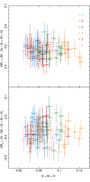
Figure 2.— The hardness ratios $\mathrm{HR_{1}}=(M-S)/(S+M+H)$ (upper panel), and $\mathrm{HR_{2}}=(H-M)/(S+M+H)$ (lower panel) plotted against the light curve of all the energy bands ($S+M+H$).

We define the count rate hardness ratios ($\mathrm{HR_{1}}$ and $\mathrm{HR_{2}}$) using the soft (S), medium (M), and hard (H) light-curve bands as follows:

$$\mathrm{HR_{1}} =\frac{M-S}{S+M+H},$$ (1)

$$\mathrm{HR_{2}} =\frac{H-M}{S+M+H},$$ (2)

The uncertainties on the hardness ratios are estimated by propagating the band errors assuming Gaussian statistics. By these definitions, as the X-ray spectra become harder, the hardness ratio $\mathrm{HR_{2}}$ increases. The disk blackbody is expected to dominate the soft band, while the powerlaw and warm absorber are the dominant features in the medium band. We note that the powerlaw dominates the hard band.

The hardness ratios $\mathrm{HR_{1}}$ and $\mathrm{HR_{2}}$ are plotted against the sum of the light curve of all the energy bands ($S+M+H$) in Figure 2. The hardness ratio $\mathrm{HR_{1}}$ increases with the count rate of the M band, and decreases with the count rate of the S band, so a decrease in $\mathrm{HR_{1}}$ may be related to a stronger soft excess of an accretion disk. In contrast, the hardness ratio $\mathrm{HR_{2}}$ decreases with the count rate of the M band and increases with the count rate of the H band, so an increase in $\mathrm{HR_{2}}$ may indicate a hardening of the powerlaw spectral index. The source tends to be slightly softer during the 4th observation (on April 13) when it has the highest luminosity. The variability of the source will be studied in a separate paper. For the time-averaged analysis, we excluded the 4th observation from the combined observations, and restrict ourselves to the five lowest flux spectra. The time-averaged spectrum of PG 1211+143 is obtained from combining $\sim 390$ ks of exposure time.

4. X-ray Spectral Analysis

We performed our X-ray spectral analysis in several steps to ensure consistent and optimal results. We assessed in § 3.1 whether the spectra can be reasonably co-added. To model the continuum, we used a phenomenological model consisting of an accretion disk model (soft band), a power-law model (hard band), and photoelectric absorption models (§ 4.1). For the absorption and emissions lines, we measure their properties first with Gaussian emission (§ 4.2) and absorption functions (§ 4.3) superimposed on the continuum. The analysis conducted in this section is intended as an additional measure to ensure that our reported results are robust to both simple (this section), and complex (§5) analysis techniques.

Table 2Best-fit Parameters for the Continuum Model and Fe Lines.

Component	Parameter	Value
	$\chi^{2}/{\rm d.o.f}$	$739/659$
tbnew	$N_{\rm H}$(cm-2 )	$2.32^{+0.48}_{-0.55}\times 10^{21}$
highecut	$E_{c}$(keV)	$4.55^{+1.16}_{-2.01}$
	$E_{f}$(keV)	$13.47_{-10.85}$
diskbb	$T_{\rm in}$(keV)	$0.064^{+0.004}_{-0.003}$
	$R_{\rm in}$(pc)	$15.96^{+16.80}_{-8.25}\times 10^{-4}$
zpowerlw	$\Gamma$	$1.77^{+0.04}_{-0.19}$
	$F$(erg cm-2 s-1)	$5.45^{+0.12}_{-0.07}\times 10^{-12}$
zgaussKα	$E$(keV)	$6.41$
(Fe K$\alpha$)	$\sigma$(keV)	$0.04$
	$F$(erg cm-2 s-1)	$3.35^{+2.31}_{-2.03}\times 10^{-14}$
zgaussHeα	$E$(keV)	$6.67$
(Fe xxv)	$\sigma$(keV)	$0.06$
	$F$(erg cm-2 s-1)	$4.87^{+3.27}_{-2.74}\times 10^{-14}$
zgaussLyα	$E$(keV)	$6.96$
(Fe xxvi)	$\sigma$(keV)	$0.06$
	$F$(erg cm-2 s-1)	$1.67^{+2.97}\times 10^{-14}$

• Notes. Redshift is fixed to $z=0.0809$.

  The Fe K$\beta$ line at 7.05 keV was estimated by tying its relative energy and absolute width to the K$\alpha$ line, and its flux to a K$\beta$/K$\alpha$ flux ratio of 0.135. The apparent inner disk radius ($R_{\rm in}$) is calculated from the norm value (see disk equations in Makishima et al., 1986; Kubota et al., 1998), adopting the luminosity distance of $D=358$ Mpc and the inclination angle of $\theta=28^{\circ}$ (Zoghbi et al., 2015). All errors are quoted at the 90% confidence level. The upper error of the highecut folding energy ($E_{f}$) is at the imposed $300$ keV limit. The lower error of the zgauss_Lyα flux ($F$) is at $0$. The use of a tbnew component here is to enable greater flexibility in the phenomenological description of the continuum shape, and should not be attributed to that amount of cold absorption in our Galaxy nor in that of PG 1211+143.

Table 3X-ray Absorption Lines in PG 1211+143 identified with Gaussian absorption functions (gabs)

Line	$E_{\rm lab}$	$\lambda_{\rm lab}$	$E_{\rm rest}$	$\lambda_{\rm rest}$	$v_{\rm out}$	$W_{\lambda}$	$v_{\rm turb}$	$\log N_{j}$
	(keV)	(Å)	(keV)	(Å)	(km s-1)	(mÅ)	(km s-1)	(cm-2)
Ne x Ly$\alpha$	1.022	12.132	1.081	11.469	$-16750^{+180}_{-630}$	$41.0\pm 6.9$	$280^{+460}_{-190}$	$17.4^{+0.1}_{-0.1}$
Ne ix He$\alpha$	0.923	13.433	0.976	12.703	$-16660^{+1290}_{-360}$	$7.5\pm 6.6$	$260^{+640}_{-190}$	$15.8^{+0.3}_{-0.9}$
Mg xii Ly$\alpha$	1.473	8.417	1.557	7.963	$-16670^{+630}_{-600}$	$20.9\pm 12.0$	$1150^{+1040}_{-870}$	$17.4^{+0.2}_{-0.4}$
Mg xi He$\alpha$	1.354	9.157	1.433	8.652	$-17070^{+450}_{-180}$	$1.7\pm 1.4$	$85^{+1230}_{-70}$	$15.5^{+0.3}_{-0.7}$
Si xiv Ly$\alpha$	2.006	6.181	2.128	5.826	$-17690^{+180}_{-30}$	$1.1\pm 1.0$	$80^{+930}_{-60}$	$16.4^{+0.3}_{-1.4}$
Si xiii He$\alpha$	1.867	6.641	1.973	6.284	$-16550^{+90}_{-570}$	$11.5\pm 6.5$	$800^{+540}_{-780}$	$17.3^{+0.2}_{-0.4}$

• Notes. The columns list the line identification, laboratory energy, laboratory wavelength, observed energy in the rest frame, observed wavelength in the rest frame, measured outflow velocity, line equivalent width, estimated turbulent velocity, and estimated ionic column of absorption line. All errors are quoted at the 90% confidence level.

4.1. Continuum Modeling

We used xspec package v. 12.9.0 (Arnaud, 1996) in isis (v. 1.6.2-35; Houck & Denicola, 2000) to model the intrinsic continuum of the combined MEG and HEG spectra in the (rest frame) energy range of 0.54–7.3 keV. We matched the continuum with a phenomenological model of $\textsf{tbnew}\times\textsf{highecut}\times(\textsf{diskbb}+\textsf{zpowerlw})$. The soft excess continuum below 1.1 keV is dominated by the xspec accretion disk model diskbb (Mitsuda et al., 1984; Makishima et al., 1986), consisting of multiple blackbodies, that has one physical parameter: the peak temperature ($T_{\rm in}$) at the apparent inner disk radius ($R_{\rm in}$) (see Makishima et al., 1986; Kubota et al., 1998). The hard excess continuum above 1.1 keV is dominated by the xspec power-law model zpowerlw, which describes the Comptonization corona of the accretion disk with the photon index ($\Gamma$). To account for foreground absorption affecting the shape of the soft X-ray continuum, we used the tbnew component (Wilms et al., 2000) for better flexibility in fitting the continuum shape in our phenomenological model. However, it does not necessarily represent any quantitative physical property of our Galaxy or the host galaxy of PG 1211+143. A high-energy exponential cutoff (highecut with cutoff energy $E_{c}$ and folding energy $E_{f}$ listed in Table 2) was also used to account phenomenologically for the curvature in the hard X-ray spectrum. Table 2 details the best fit parameters based on this model.

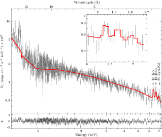
Figure 3.— The X-ray spectrum taken with the Chandra-HETGS in 2015 April averaged over 390 ks (i.e., excluding the 4th observation). The upper panel shows the first-order spectrum (black line) and the best-fitting continuum model plus iron emission lines (red line; tbnew *highecut *(diskbb +zpowerlw +$\sum$ zgauss)), while the lower panel plots the $\chi^{2}$ residuals between the observation and the best-fitting model.

4.2. Iron Emission Lines

To fit the iron emission lines, we added four Gaussian components (zgauss) at 6.4 keV (Fe K$\alpha$), 6.67 keV (Fe He$\alpha$), 6.96 keV (Fe Ly$\alpha$), and 7.05 keV (Fe K$\beta$) in the rest frame to the continuum model as follows: $\textsf{tbnew}\times\textsf{highecut}\times(\textsf{diskbb}+\textsf{zpowerlw}+\sum_{i=1}^{4}\textsf{zgauss}(i))$.

As seen in Figure 3, the data are consistent with three Gaussian lines at energies between 6 keV and 7 keV, namely the K$\alpha$ fluorescent iron line at 6.4 keV, the He$\alpha$ iron line at 6.67 keV, and the Fe Ly$\alpha$ iron line at 6.96 keV blended with K$\beta$ fluorescent iron lines at 7.05. To measure the Ly$\alpha$ line flux correctly, we set the K$\beta$ line flux to the theoretical iron K$\beta$/K$\alpha$ flux ratio of 0.135 (e.g. see Palmeri et al., 2003), then estimated the Ly$\alpha$ line in the presence of a possible K$\beta$ contribution, whose absolute width and relative energy were also tied to the Fe K$\alpha$. The lines that we associate with fluorescent iron and He-like iron emission are significantly detected with positive equivalent widths.

4.3. Ionized Absorption Lines

Strong absorption lines of key H- and He-like ions were visually identified initially, and we modeled them using a series of Gaussian absorption functions (gabs) with physical properties listed in Table 3. For thoroughness, we also identified additional potential spectral features using a blind line search described in the Appendix. For these key lines, we obtained the ionic column densities ($N_{j}$) from the following relationship between $W_{\lambda}$ and $N_{j}f_{jk}$ for the unsaturated absorption lines (Spitzer, 1978, Ch. 3):

$$\frac{W_{\lambda}}{\lambda}=\frac{\pi e^{2}}{m_{e}c^{2}}N_{j}\lambda f_{jk},\\$$ (3)

where $W_{\lambda}$ is the line equivalent width, $\lambda$ the wavelength, $N_{j}$ the ionic column density, $f_{jk}$ the oscillator strength of the relevant transition taken from the atomic database AtomDB (v. 2.0.2; Foster et al., 2012), $c$ the speed of light, $m_{e}$ the electron mass, and $e$ the elementary charge.

Table 3 lists the measured outflow velocity ($v_{\rm out}$). and the line equivalent width ($W_{\lambda}$) in mÅ from the absorption lines. The turbulent velocity width is estimated from the FWHM ($=2\sqrt{2\ln 2}\sigma$, where $\sigma$ is the velocity dispersion) of the line profile using $v_{\rm turb}={\rm FWHM}/2\sqrt{\ln 2}$. The ionic column density is derived using equation (3).

5. Photoionization Modeling

We next proceed with more detailed photoionization analysis using the code xstar (v 2.2; Kallman et al., 1996; Kallman & Bautista, 2001; Kallman et al., 2004, 2009), primarily developed for X-ray astronomy. This code solves the radiative transfer of ionizing radiation in a spherical gas cloud under a variety of physical conditions for astrophysically abundant elements, calculates ionization state and thermal balance, and produces the level populations, ionization structure, thermal structure, emissivity and opacity of a gas with specified density and composition, including the rates for line emission and absorption from bound-bound and bound-free transitions in ions. It utilizes the atomic database of Bautista & Kallman (2001), containing a large quantity of atomic energy levels, atomic cross section, recombination rate coefficients, transition probabilities, and excitation rates.

We assumed a spherical geometry with a covering fraction of $C_{f}=\Omega/4\pi=0.5$, which is typical of the ionized absorbers in AGNs (Tombesi et al., 2010). Fundamental parameters in photoionization modeling are the total gas number density $n$ (in cm^-3), the total hydrogen column density $N_{\rm H}=n_{H}V_{f}\triangle r$ (in cm^-2), the ionization parameter $\xi=L_{\rm ion}/n_{H}r^{2}$ (in erg cm s^-1; Tarter et al., 1969), and the turbulent velocity $v_{\rm turb}$ (km s^-1), where $L_{\rm ion}$ (in erg s^-1) is the ionizing luminosity between 13.6 eV and 13.6 keV (i.e. 1 and 1000 Ryd), $V_{f}$ is the volume filling factor of the ionized gas, and $r$ and $\triangle r$ are the distance from the ionizing source and the thickness of the ionized gaseous shell (in units of cm), respectively. We set the initial gas temperature to the typical value of $T_{\rm init}=10^{6}$ K (Nicastro et al., 1999; Bianchi et al., 2005), and allowed the code to calculate it based on the thermal equilibrium of gas. We generated grids of xstar models (see § 5.2) using an ionizing spectral energy distribution (SED) described in § 5.1 (see also Figure 4).

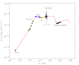
Figure 4.— Observed and interpolated baseline SED (solid red line) used for photoionization modeling of PG 1211+143. The solid points are (1) the radio data at 20 cm taken with the VLA, and (2) infrared measurements (JHKs, 3.4, 4.6, 12, 22, 70, 100, 160, 250, 350, and 500 $\mu$m) from Petric et al. (2015). Spectra are also shown (in solid black and gray lines), and are (1) the archival UV data taken with the HST-FOS in 1991 April 1(PID 1026, PI: Burbidge), (2) our recent FUV observations with the HST-COS, and (3) the Chandra-HETGS.

5.1. Spectral Energy Distribution

Since it was found by Lee et al. (2013) that the UV continuum is an important component of the ionizing flux, we employed a similar methodology here to generate radio, infrared, UV, and X-ray components of the ionizing SED for the photoionization modeling of the warm absorber in PG 1211+143. Although the combined UV and X-ray continua are expected to be the main source of the ionizing radiation, we have used the entire ranges from radio to X-ray to construct the SED (see Figure 4). The archival UV data taken with the HST-FOS in April 1991 (G130H, G190H, and G270H), together with our HST-COS time-averaged FUV spectrum (G140L) observed simultaneously with Chandra in April 2015, were used to construct the SED. We utilized our Chandra MEG and HEG data to make X-ray continuum regions (0.5–8 keV) of the ionizing SED. The soft X-ray continuum was extrapolated as a power law at energies below 0.5 keV to the point at which it meets the high-energy extrapolation of the UV powerlaw. We also used the radio fluxes at 20 cm (1.5 GHz), $S_{\nu}=2$ mJy, measured with the VLA (§ 2.3), the near-infrared (NIR) measurements (JHKs) from the Two Micron All Sky Survey (2MASS), the mid-infrared (MIR) measurements at 3.4, 4.6, 12, and 22 $\mu$m from the Wide-field Infrared Survey Explorer (WISE), and the far-infrared (FIR) measurements at 70, 100, 160, 250, 350, and 500 $\mu$m from the ESA Herschel Space Observatory (Petric et al., 2015). Similarly, the radio, NIR, MIR, and FIR band points were connected to each other. However, the ionizing SED is mainly characterized by the UV and X-ray spectra without the emission and absorption lines. The IR, optical and UV data were first dereddened using $R_{\rm V}=3.1$ and $E({\rm B-V})=0.035$ (Schlafly & Finkbeiner, 2011), and placed in the rest frame. The X-ray data were also corrected for the foreground Galactic absorption.

The resulting intrinsic SED is shown in Figure 4 with associated bands (points) and composite spectra, connecting the IR, UV and X-rays regions (solid line). The intrinsic SED is then used to generate grids of photoionization models that are fitted to the X-ray absorption lines. To obtain the ionizing luminosity, we integrate the interpolated baseline SED between $\nu=3.29\times 10^{15}$ and $3.29\times 10^{18}$ Hz (i.e., 1–1000 Ryd), finding $\int F_{\nu}\,d\nu=1.035\times 10^{-10}$ erg cm^-2 s^-1, which yields $L_{\rm ion}=1.587\times 10^{45}$ erg s^-1 at the luminosity distance of 358 Mpc ($H_{0}=73$ km s^-1 Mpc^-1, $\Omega_{m}=0.27$, and $\Lambda_{0}=0.73$; $z=0.082$ corrected to the microwave background radiation reference frame). Previously, the ionizing luminosity (1–1000 Ryd) of $3.8\times 10^{45}$ erg s^-1 was estimated from XMM–Newton observation (Pounds et al., 2016b).

5.2. Photoionization Tabulated Grids

Table 4Parameter ranges for xstar Photoionization Model Grids.

Parameter	Value	Interval Size
$L_{\rm ion}$ ($10^{38}$ erg s-1)	$1.587\times 10^{7}$	–
$T_{\rm init}$ ($10^{4}$ K)	$100$	–
$\log n$ (cm-3)	$8\cdots 14$	$1.0$
$\log N_{\rm H}$ (cm-3)	$18\cdots 25$	$0.5$
$\log\xi$ (erg cm s-1)	$-2\cdots 5$	$0.25$
$v_{\rm turb}$ (km s-1)	$100\cdots 500$	$100.0$
$A_{\rm Fe}$	$1.0$	–
$C_{f}=\Omega/4\pi$	$0.5$	–

• Notes. Logarithmic interval sizes are chosen for the total gas number density ($n$), the total hydrogen column density ($N_{\rm H}$), the ionization parameter ($\xi=L_{\rm ion}/n_{H}r^{2}$), while a linear interval size is chosen for the turbulent velocity ($v_{\rm turb}$). The ionizing luminosity ($L_{\rm ion}$) is derived from an integration (1–1000 Ryd) of the interpolated baseline SED shown in Figure 4. The initial gas temperature ($T_{\rm init}$) is set to the typical value of $10^{6}$ K (Nicastro et al., 1999; Bianchi et al., 2005), while the code adjusts it based on the thermal equilibrium. The covering fraction is fixed to the typical value of the X-ray absorbers ($C_{f}=0.5$; Tombesi et al., 2010).

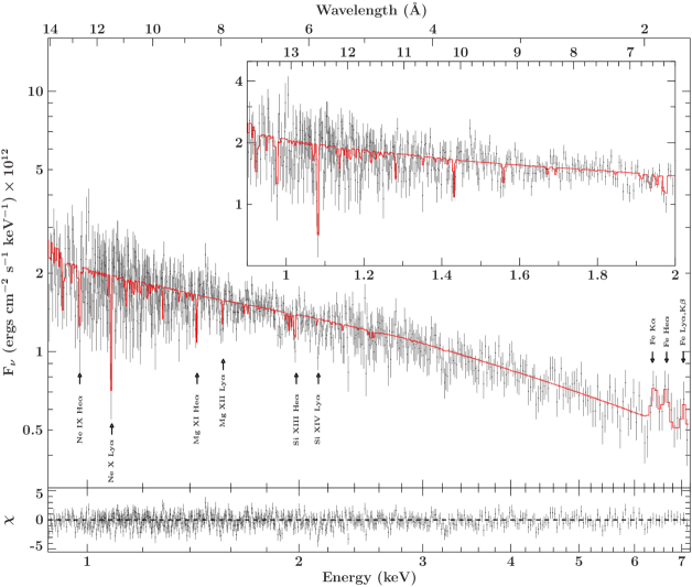
Figure 5.— Chandra HETGS spectrum for PG 1211+143 fit with the xstar warmabs model (see Table 5). The lower panel plots the $\chi^{2}$ residuals between the observation and the model.

We used the ionizing SED made in § 5.1 to generate grids of xstar models. We utilized mpi_xstar (Danehkar et al., 2018) that allows parallel execution of multiple xstar runs on a computer cluster (in this case, the odyssey cluster at Harvard University). It employs the xstar2table script (v. 1.0) to produce multiplicative tabulated model files: an absorption spectrum imprinted onto a continuum (xout_mtable.fits), a reflected emission spectrum in all directions (xout_ain.fits), and an emission spectrum in the transmitted direction of the absorption (xout_aout.fits). The first and second tabulated model files are used as absorption and emission components of the ionized outflows (or infalls) in spectroscopic analysis tools. Table 4 lists the parameters used for producing xstar model grids. To cover the possible range of physical conditions, we initially considered a large range of gas densities $n$ from $10^{8}$ to $10^{14}$ cm^-3, column densities $N_{\rm H}$ from $10^{18}$ to $10^{25}$ cm^-2, ionization parameters $\xi$ from $10^{-2}$ to $10^{5}$ erg cm s^-1, and turbulent velocities of 100–500 km s^-1, for use in spectral fitting.

We computed a grid of $15\times 29$ xstar models on the two-dimensional $N_{\rm H}$–$\xi$ plane, sampling the fundamental parameter space with 15 logarithmic intervals in the column density (from $\log N_{\rm H}=18$ to $25$ cm^-2 with the interval size of $0.5$) and 29 logarithmic intervals in the ionization parameter (from $\log\xi=-2$ to $5$ erg cm s^-1 with the interval size of $0.25$), assuming a gas density of $n=10^{12}$ cm^-3. For diagnostic purposes, we have initially constructed some grids with the same $N_{\rm H}$–$\xi$ parameter space for $\log n=8$–$14$ cm^-3 (interval size of $1$), and $v_{\rm turb}=100$–$500$ km s^-1 (interval size of $100$). However, we found that results were indistinguishable for this wide range of the gas density in highly-ionized absorbers. Hereafter, all xstar models correspond to a gas density of $n=10^{12}$ cm^-3.

The turbulent velocity is another important parameter in photoionization modeling. An increase in the turbulent velocity increases the equivalent width of an absorption line for a given column density of each ion. To estimate equivalent widths correctly, the velocity width, which is associated with line broadening, must be measured precisely. The high spectral resolution of MEG and HEG data allows for the possibility of determining the velocity width. However, due to insufficient counts, our HETGS observations pointed to a wide range of velocity widths with high uncertainties, so we could not measure the exact value of $v_{\rm turb}$ for each ion. From the line width measurements (see Table 3), we adopted a velocity turbulence of $v_{\rm turb}=200$ km s^-1 for the warm absorber, which approximately corresponds to the HETGS optimal spectral resolution.

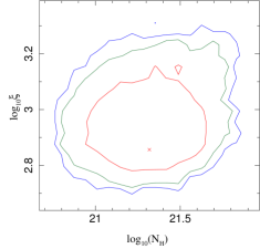
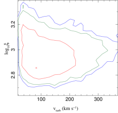
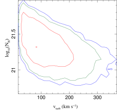
Figure 6.— The 1-sigma (68%), 2-sigma (95%), and 3-sigma (99%) confidence contours of the logarithm of the ionization parameter ($\log\xi$) vs. the logarithm of the column density ($\log N_{\rm H}$; left), the logarithm of the ionization parameter ($\log\xi$) vs. the turbulent velocity ($v_{\rm turb}$; middle), and the logarithm of the column density ($\log N_{\rm H}$) vs. the turbulent velocity ($v_{\rm turb}$; right) of the ionized absorber with the best-fitting parameters listed in Table 5, respectively. The cross sign shows the best-fitting values in each panel.

We proceeded to fit the combined MEG and HEG data shown in Figure 5, multiplying our continuum model by the xstar tabulated grids produced from the ionizing SEDs in § 5.1. There are a total of two free parameters in the tabulated grid fitting, namely, the ionization parameter $\xi$ and column density $N_{\rm H}$ of the ionized absorber. Using the base continuum model described in § 4.1, the model for the spectra containing 1 ionized absorber and 4 Fe emission lines are implemented as follows: $\textsf{tbnew}\times\textsf{highecut}\times(\textsf{diskbb}+\textsf{zpowerlw}+\sum_{i=1}^{4}\textsf{zgauss}(i))\times\textsf{xstar\_absorber}$. These models successfully described the data with an ionization parameter of $\log\xi=2.9\pm 0.1$ and a column density of $N_{\rm H}=(2.4\pm 0.6)\times 10^{21}$ (90% confidence levels), with an observed redshift of $(0.0201\pm 0.0005)c$. The model with these parameters has a goodness-of-fit of $\chi^{2}/{\rm d.o.f}=738/661$. These results allowed us to refine our parameter estimations in performing the warmabs model fitting described in the subsequent section.

5.3. Photoionization Analytic Modeling

We constrained the properties of potential ionized absorbers using the xstar analytic model warmabs, relying on all atomic level populations calculated by xstar using the same UV–X-ray ionizing SED from § 5.1. Fitting the spectrum with the tabulated grids (see § 5.2) is much quicker than the warmabs analytic modeling. However, parametric intervals used in the computation of the model grids (see interval sizes in Table 4) could add large uncertainties to derived parameters. Hence, we also used the analytic model to put more accurate constraints on the ionization state and column density of the warm absorbing gas, as well as to explore any variations in elemental abundances. As this approach is computationally expensive, we utilized the parameters determined from the xstar table model grids in § 5.2 as initial values, and employed warmabs only to make finer estimations of the physical conditions.

For the soft excess, we again use an absorbed disk component. The high-ionization lines visible in the spectrum (c.f. Table 3) clearly require a highly ionized warmabs component. Given that the tbnew component in our phenomenological model (§4.2) shows more absorption than expected for foreground Milky Way absorption ($N_{\rm H}=2.6\times 10^{20}$ cm^-2; Wakker et al., 2011), we have tried three different options for additional absorption in PG 1211+143. Specifically, we considered (1) a neutral absorber (tbnew) at the PG 1211+143 systemic redshift, (2) a mildly ionized warmabs model (also at the PG 1211+143  systemic redshift), and (3) a low-ionization warmabs model at the same observed redshift as the high-ionization warmabs component. For this third possibility we also tied the abundance and turbulent velocity parameters to those of the high-ionization warmabs component.

Table 5Best-fitting parameters for the xstar warmabs model, the continuum model and iron lines obtained using the isis emcee hammer routine.

Component	Parameter	Value
	$\chi^{2}/{\rm d.o.f}$	$610/614$
highecut	$E_{c}$(keV)	$1.4^{+0.3}_{-0.4}$
	$E_{f}$(keV)	$11.3^{+3.5}_{-0.8}$
diskbb	$T_{\rm in}$(keV)	$0.096^{+0.002}_{-0.010}$
	Norm	$1.2^{+1.5}_{-0.3}\times 10^{4}$
zpowerlw	$\Gamma$	$1.55^{+0.04}_{-0.07}$
	Norm ($\gamma$ keV-1 cm-2)	$1.38^{+0.04}_{-0.09}\times 10^{-3}$
zgaussKα	$E$(keV)	$6.41^{+0.06}_{-0.05}$
(Fe K$\alpha$)	$\sigma$(keV)	$0.004^{+0.13}$
	Norm ($\gamma$ cm-2 s-1)	$3.6^{+3.2}_{-2.0}\times 10^{-6}$
zgaussHeα	$E$(keV)	$6.66^{+0.12}_{-0.09}$
(Fe xxv)	$\sigma$(keV)	$0.06^{+0.22}_{-0.02}$
	Norm ($\gamma$ cm-2 s-1)	$5.2^{+6.6}_{-3.9}\times 10^{-6}$
warmabs	$\log n$ (cm-3)	12.0
	$\log N_{\rm H}$ (cm-2)	$21.47^{+0.18}_{-0.58}$
	$\log\xi$ (erg cm s-1)	$2.87^{+0.32}_{-0.10}$
	$v_{\rm out}$ (km s-1)	$-17300^{+100}_{-130}$
	$v_{\rm turb}$ (km s-1)	$90^{+210}_{-60}$
	$A_{\rm Ne}$	$0.6^{+2.0}_{-0.2}$
	$A_{\rm Mg}$	$1.5^{+3.2}_{-0.4}$
	$A_{\rm Si}$	$3.0^{+4.8}_{-1.1}$
	$A_{\rm S}$	$0.6^{+5.3}_{-0.4}$
	$A_{\rm Fe}$	$1.2^{+1.6}_{-0.6}$
warmabs	$\log N_{\rm H}$ (cm-2)	$21.08^{+0.10}_{-0.62}$
	$\log\xi$ (erg cm s-1)	$1.29^{+0.34}_{-0.29}$

• Notes. The total gas number density ($n$) is fixed to the typical value for AGN ionized absorbers. The total hydrogen column density ($N_{\rm H}$), ionization parameter ($\xi=L_{\rm ion}/n_{H}r^{2}$), Doppler velocity ($v_{\rm out}$), turbulent velocity ($v_{\rm turb}$), and elemental abundances ($A$) are free parameters estimated by the xstar analytic warmabs modeling. The chemical abundances are with respect to the solar values defined in Wilms et al. (2000). The second warmabs component has all parameters, save ionization parameter and column, tied to those of the more highly ionized absorber. All uncertainties are estimated at the 90% confidence level.

All three of these possibilities resulted in essentially identical parameters for the highly ionized absorber. None of the three possibilities produced identifiable spectral features, but rather affected the shape of the low-energy X-ray continuum. Differences among the fits were primarily restricted to the soft excess parameters, with subtler differences in the highest and zpowerlw parameters. In what follows, we only present results for option (3), the additional low-ionization component at the observed redshift of the high-ionization component. However, we consider the high-ionization component to be the only one with well-measured parameters, and we only discuss its physical implications.

In our fits, we used the solar abundances defined by Wilms et al. (2000), and adjusted the elemental abundances and the turbulent velocity to match the absorption lines. The best-fitting parameters derived from our model fits are listed in Table 5. We determined the fit parameter confidence intervals by employing the isis emcee hammer routine, which is an implementation of the Markov Chain Monte Carlo (MCMC) Hammer algorithm of Foreman-Mackey et al. (2013), and now included in the Remeis ISISscripts. The MCMC approach allowed us to improve the best-fitted values of the ionization parameter ($\xi$), the column density ($N_{\rm H}$), the turbulent velocity ($v_{\rm turb}$), and the chemical composition of the warmabs model as well as other phenomenological model parameters (continuum and iron lines) listed in Table 5 (the fits, however, are not very sensitive to the chemical composition). Figure 6 shows the 1-sigma (68%), 2-sigma (95%), and 3-sigma (99%) confidence contours of $\log\xi$ versus $\log N_{\rm H}$, $\log\xi$ versus $v_{\rm turb}$, and $\log N_{\rm H}$ versus $v_{\rm turb}$. There is a slight anti-correlation between the absorber column and turbulent velocity (somewhat expected to fit the equivalent widths of the detected features). Overall, the main absorber parameters are well constrained.

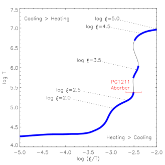
Figure 7.— Thermal stability curve for $n_{\rm H}=10^{12}$ cm^-3 produced using the xstar model associated with the UV–X-ray ionizing SED shown in Figure 4. It shows the distribution of equilibrium temperature $\log T$ as a function of $\log(\xi/T)$. The thick solid lines in the curves correspond to the regions with the thermally stable gas. The best-fitting $\xi$ value of the ionized absorber component is labeled as PG1211 with its corresponding error bar at the 90% confidence level.

5.4. Thermal Stability

The photoionization model fitting yielded the ionized absorber with the physical conditions listed in Table 5, hydrogen-equivalent column density $N_{\rm H}$ (in cm^-2) and ionization parameter $\log\xi$ (in erg cm s^-1), which are required to reproduce the blueshifted absorption features in the spectrum of PG 1211+143.

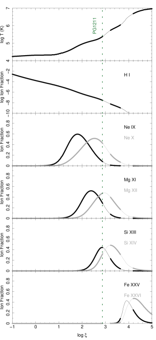
Figure 8.— The distribution of temperature $\log T$ (top panel) and the ion fraction distributions of the neutral hydrogen (H i), the He-like (black line) and H-like (gray line) ions of the relevant elements (Ne, Mg, Si and Fe) as a function of ionization parameter $\log\xi$ produced using the xstar model with the ionizing UV–X-ray SED shown in Figure 4. The thick solid lines in the curves correspond to the regions with the thermally stable gas. The vertical dot line (labeled as PG1211) is associated with the xstar warm absorber with parameters listed in Table 5. We note that while Fe xxv  is included here, it was not detected with any significance in this Chandra observation. The gas density is chosen to be $n_{\rm H}=10^{12}$ cm^-3. As can be seen, H i can exist even at the high ionization required by the detected X-ray lines, lending extra credence to our findings that the $\rm\sim 16980\,km\,s^{-1}$ outflow we detect with Chandra and HST are likely associated.

The stability curve, in which temperatures ($T$) of clouds are plotted against their pressures ($\xi/T$), is an effective theoretical tool to illustrate the thermal stability of ionized absorbing clouds (Krolik et al., 1981; Reynolds & Fabian, 1995; Krolik & Kriss, 2001; Chakravorty et al., 2009, 2013). The absorber is thermally stable where the slope of the stability curve is positive and where the heating and cooling mechanisms are in equilibrium. Figure 7 shows the stability curve generated using the xstar model for a gas density $n_{\rm H}=10^{12}$ cm^-3 and the corresponding parameters specified in § 5.3. As can be seen, the ionized absorber is just at the edge of the thermally stable region. Interestingly, in the prior XMM-Newton observation in 2014, when PG 1211+143 was twice as bright, the ionization parameter $\xi$=3.4 (Pounds et al., 2016b), consistent with the increased brightness, and lying on the next-highest stable portion of the curve.

Figure 8 shows the distribution of temperature $\log T$, the neutral hydrogen (H i), and ion fractions of the He-like and H-like ions of the relevant elements (Ne, Mg, Si and Fe) with respect to the ionization parameter $\log\xi$, from our xstar model. The distribution of temperature and ion fractions typically depend on the ionization parameter, the gas density, and the ionizing SED (Kallman & Bautista, 2001). The thick solid lines correspond to the range where the absorbing gas is thermally stable. This figure further shows that both the X-ray detected ions and the UV absorber detected in H i  can all coexist in a single ionization zone at the same velocity.

6. HST-COS Results: Evidence for a Corresponding UV Absorber

Our HST-COS observations reveal a previously unknown, weak, broad, blueshifted Ly$\alpha$ absorption feature consisting of two blended components, as shown in Figure 9. Kriss et al. (2018) discuss in detail the analysis of the UV data in general and this feature specifically. They find an average outflow velocity of $v_{\rm out}=-16\,980\pm 40~{}\rm km~{}s^{-1}$ ($z_{\rm out}=-0.0551$) with a FWHM of $1080\pm 80~{}\rm km~{}s^{-1}$. Both the HST-detected outflow velocity and width are consistent with the strongest X-ray absorption features, giving additional credence to the reality of such a high velocity outflow. In addition to the Ly$\alpha$ feature in the G130M spectrum, we also detect Ly$\beta$ at the same velocity in the G140L spectrum, albeit at lower significance. No other UV ions are detected, including high-ionization species such as C iv, N v or O vi.

Several other narrow absorption lines appear in the UV spectrum of PG 1211+143 embedded within the profile of the newly detected broad Ly$\alpha$ absorption feature. These include foreground interstellar absorption in the N v doublet, as well as the previously known features from the foreground intergalactic medium (IGM) (Tilton et al., 2012). We can safely conclude that these narrow features are not associated with the outflow from PG 1211+143 because they do not share any of the characteristics typical of absorption lines associated with AGN outflows– they are not variable in strength, and they fully cover the source. The Ly$\alpha$ to Ly$\beta$ optical depth ratios (Danforth & Shull, 2008; Tilton et al., 2012) are consistent with their Doppler widths, which at $\sim 35$ km s^-1 are typical of other IGM Ly$\alpha$ absorbers.

The similar depths of the broad Ly$\alpha$ and Ly$\beta$ features in our spectra indicate that they are saturated, so that the UV absorber only partially covers the continuum source. Using the depth at the center of the Ly$\alpha$ absorption feature, we measure a covering fraction of $C_{f}=0.30\pm 0.04$. Since the lines are saturated, we cannot measure an accurate column density, but we can set a lower limit assuming a covering factor of unity and integrating across the apparent optical depth of the line profile (e.g., Hamann et al., 1997). This gives $\log N_{\text{H\,{\sc i}}}\gtrsim 14.5$ cm^-2.

Figure 9.— HST-COS G130M spectrum of PG 1211+143 in the wavelength range covering the broad Ly$\alpha$ absorption line profile, the IGM Ly$\alpha$ lines (Penton et al., 2004) and interstellar N v and S ii lines, adapted from Kriss et al. (2018). The lower horizontal axis is the observed wavelength in Ångstrom. The upper horizontal axis is the outflow velocity of Ly$\alpha$ relative to a systemic redshift of $z=0.0809$.

Despite the high ionization of the X-ray absorber detected at the same outflow velocity, our photoionization models predict a small residual column density of neutral hydrogen. At our best-fit $\log\xi=2.87$, the ionization fraction of H i is $2.99_{-2.40}^{+1.49}\times 10^{-8}$. For our best-fit total hydrogen column density of $\log N_{\rm H}=21.47_{-0.58}^{+0.18}$ cm^-2, we predict $\log N_{\text{H\,{\sc i}}}=13.95^{+0.26}$ cm^-2, roughly consistent with our measured lower limit of $\log N_{\text{H\,{\sc i}}}\gtrsim 14.5$ cm^-2. As Kriss et al. (2018) show, the Ly$\alpha$ profile actually consists of two blended components, so it is possible that the X-ray UFO is associated with only a portion of the Ly$\alpha$ absorption profile. This would also explain the narrow turbulent velocity we find for the X-ray absorber compared to the Ly$\alpha$ absorber.

All other UV ions are predicted to have column densities at least three orders of magnitude lower, rendering them undetectable even in our high S/N HST-COS spectra.

7. VLA Results: Evidence for a Jet?

The radio emission from PG 1211+143 is compact at all the frequencies and resolutions we have studied. In our deep K-band image, fitting a Gaussian to the source gives a best-fitting major axis of 22 mas, corresponding to 33 pc at the distance of the quasar assuming the cosmological parameters from the previous section. Given that residual phase uncertainties can induce blurring in a point-like source, this should probably be taken as an upper limit on the size of the source.

The flux densities measured from the various (non-simultaneous) radio data available to us are summarized in Table 6. In all cases these are the integrated flux densities of a Gaussian fitted to the data around the position of the quasar using the AIPS task JMFIT.

Kellermann et al. (1994) report a 5-GHz flux density of $0.80\pm 0.1$ mJy for the source in observations taken in 1983, so, taking this with our two C-band flux densities, there is some modest evidence for a slow evolution of the apparent luminosity of the source at the 10% level on a timescale of decades. We have no information on whether the fast variability of the source seen in the X-rays is also present in the radio.

The radio SED of the source is interesting, because, assuming that variability can be neglected, we see a spectral index $\alpha$ (defined in the sense $S\propto\nu^{\alpha}$) of $-0.49\pm 0.06$ between L and C-band, $-0.79\pm 0.03$ between C and K-band, and $-1.0\pm 0.4$ internal to the K-band (using the ‘lower’ and ‘upper’ halves of the band). Thus all the SED measurements are consistent with coming from optically thin synchrotron emission, with a steeper spectrum at higher frequencies presumably due to radiative losses. If we further assume that all the emission we see comes from a region of less than 30 pc in size, this gives a consistent picture in which the radio emission comes from an optically thin region: for example, assuming a prolate ellipsoidal emission region with major axis 22 mas and minor axis half the major axis, and taking $E_{\rm min}$ for the relativistic electrons to be 5 MeV, the minimum energy in the synchrotron-emitting particles and field would be around $5\times 10^{53}$ erg, the equipartition field strength would be of order 700 $\mu$G, and self-absorption would be expected to become important at frequencies below a few hundred MHz. The source would need to be a factor of a few smaller before self-absorption would be expected to affect the lowest frequencies we observe. If the source is strongly projected, as might be expected for an object that appears as a quasar, then these constraints are relaxed, since the true physical size is $\lesssim 30/\sin\theta$ pc where $\theta$ is the angle to the line of sight.

Table 6Radio flux densities for PG 1211+143

Band	Central freq.	Date	Flux density
	(GHz)		(mJy)
L (FIRST a)	1.4	$1999$	$2.10\pm 0.17$
C	4.9	1993 May 02	$0.95\pm 0.07$
C	6	2015 Jun 18	$1.032\pm 0.015$
K	22	2015 Jun 18	$0.370\pm 0.011$
K (lower)	20	2015 Jun 18	$0.384\pm 0.013$
K (upper)	24	2015 Jun 18	$0.320\pm 0.017$

• ^a Data retrieved from The VLA FIRST Survey

If we further assume that such a compact region is expanding at $\sim c$, then the minimum energy in the synchrotron-emitting plasma would imply jet kinetic powers $>3\times 10^{44}$ erg s^-1, which, although high, is substantially less than the radiative luminosity of the quasar, and again this number would be reduced by projection, or by assuming slower expansion speeds. It should be noted, though, that the numerator of this calculation is the minimum energy, and departures from equipartition, which would imply higher energy densities in the synchrotron-emitting material, are very common in larger-scale radio sources. Given these uncertainties, it certainly does not seem impossible to imagine a scenario in which the shock driven by the jet/lobe system responsible for the radio emission gives rise to the fast bulk outflows detected in the X-ray and UV spectra. Although the shock driven by the jet provides the acceleration mechanism in this scenario, we would still expect the shocked gas to be photoionized by the central continuum source, consistent with our photoionization model for the absorption. Tombesi et al. (2014) have shown that both radio jets and UFOs can co-exist in AGN, and may even be related. Testing such a model would require very long baseline interferometric (VLBI) imaging sensitive enough to detect and resolve the radio emission at mas resolution.

8. Discussion

Our simultaneous Chandra and HST observations are the first definitive confirmation of an ultra-fast outflow detected simultaneously in both X-ray and UV spectra. Highly ionized gas at an outflow velocity of $-17\,300~{}\rm km~{}s^{-1}$ ($-0.0577c$) in our Chandra spectrum is an excellent match to the broad Ly$\alpha$ absorption at $-16\,980~{}\rm km~{}s^{-1}$ ($-0.0551c$) in our HST-COS spectrum (Kriss et al., 2018). Previous X-ray observations of PG 1211+143 found evidence for outflows clustered near several different velocities. In the original observations using XMM-Newton, Pounds et al. (2003) identified an ultra-high velocity outflow at $\sim-0.09c$ ($-27\,000~{}\rm km\,s^{-1}$), detected only in very highly ionized gas producing the Fe xxvi K$\alpha$ transition. Re-analysis of this same data set reaffirmed the detection of ultra-high velocity gas, but at $-0.14\pm 0.01~{}c$, with additional high-ionization lines at $\sim-0.07c$ (Pounds, 2014). Most recently, the deepest observations to date of PG 1211+143 using XMM-Newton ($\sim$450 ks) in 2014 again detected ultra-high velocity gas at $-0.129c$ and high-velocity gas at $-0.066\pm 0.003c$ (Pounds et al., 2016b; Reeves et al., 2018). The UFO at $-0.129~{}c$ is not seen in contemporaneous NuSTAR data (Zoghbi et al., 2015), but a combined analysis of the XMM-Newton and NuSTAR spectra show that the spectral structure around 7 keV is quite complex. Pounds et al. (2016b) show that the $-0.129~{}c$ feature is quite variable, both in column density and in ionization parameter. Given the complexity of the spectrum around 7 keV and the lower column density of the $-0.129c$ feature in 2014, from a joint analysis of the NuSTAR and XMM-Newton spectra, Lobban et al. (2016) argue that it is not surprising that it is not detectable in the NuSTAR data.

Subsequent analysis of the 2014 XMM-Newton RGS data by Reeves et al. (2018) shows that two lower-ionization, lower velocity absorbers are also present with velocities of $-0.062\pm 0.001c$ ($v_{\rm out}=-18\,600\pm 300$ km s^-1) and $-0.059\pm 0.002c$ ($v_{\rm out}=-17\,700\pm 600$ km s^-1), the latter of which is a good match to the $-17\,300$ km s^-1 ($-0.0577c$) warm absorber we detect in our Chandra spectrum. However, the absorber we detect is slightly lower in ionization (log $\xi=2.87^{+0.32}_{-0.10}$ vs. log $\xi=3.4\pm 0.1$), and nearly an order of magnitude lower in column density ($N_{\rm H}=3\times 10^{21}$ cm^-2 vs. $1\times 10^{22}$ cm^-2). Both the velocity and the lower total column density are compatible with the Ly$\alpha$ absorption detected in the simultaneous HST-COS spectrum (Kriss et al., 2018).

Simultaneously detecting the same kinematic outflow with both Chandra and HST provide the first opportunity to assess the physical characteristics of an ultra-fast outflow using both X-ray and UV spectra. However, we note that this absorber is fairly high ionization, both in the X-ray and the UV. This is consistent with our detection of only broad Ly $\alpha$ in our UV spectrum–the ionization is too high to produce significant populations of the usually seen UV ions. Kriss et al. (2018) also do not detect UV absorption lines that might be associated with a lower-ionization warm absorber, either in the COS spectrum or in archival spectra from earlier epochs. This is consistent with no evidence for a lower-ionization X-ray WA in PG 1211+143. Despite the curvature in the Chandra spectrum that might suggest a lower-ionization absorber, there are no detected absorption lines, either in the X-ray nor in the UV. The UV is especially sensitive in this regard. All X-ray WAs also show UV absorption in C iv (Crenshaw et al., 2003) or O vi (Dunn et al., 2008). Although Tombesi et al. (2013) has suggested that WAs may be a lower-ionization manifestation of the same wind structure represented by UFOs, but at larger distances from the black hole, this has been disputed by Laha et al. (2016). The lack of a low-ionization absorber in PG 1211+143, unfortunately, does not have much bearing on this dispute since $\sim 30$% of sources containing UFOs do not have associated WAs.

The lower ionization state of the gas in our Chandra observation is expected, given the $\sim 2\times$ lower X-ray flux in 2015 compared to 2014. Such an ionization response has been seen in longer, more extensive observations of other UFOs. The long XMM-Newton observation of IRAS 13224$-$3809 shows variability of its high-ionization UFO in concert with variations in the X-ray flux (Parker et al., 2017a, b), consistent with the response of photoionized gas. However, we also see a significant decrease in total column density, $\log N_{\rm H}=21.5$ cm^-2 compared to $\log N_{\rm H}=22.0$ cm^-2 Reeves et al. (2018) and $23.3$ cm^-2 Pounds et al. (2016a) in 2014. Column density variations are also seen in other UFOs such as PDS 456, where Reeves et al. (2016) suggest that the broad, variable soft X-ray absorption lines they see are due to lower-velocity clumps in the overall outflow. In PG 1211+143 itself, Pounds et al. (2016a) find that both ionization and column density vary in the 2014 XMM-Newton observation.

Although in §7 we have presented a notional model for driving the observed outflow in PG 1211+143 via shocks from a jet associated with the radio source, the most popular mechanism for explaining ultra-fast outflows is via a wind driven from the accretion disk. In both radiative and MHD models of accretion disk winds, the velocity of the outflow is expected to reflect the orbital velocity at which the wind was launched (e.g., Proga et al., 2000; Proga, 2003; Fukumura et al., 2010a; Kazanas et al., 2012). Based on reverberation mapping, the black-hole mass of PG 1211+143 is $1.46\times 10^{8}~{}M_{\odot}$ (Peterson et al., 2004) (although this is poorly constrained). For an orbital velocity of $17\,300$ km s^-1, the wind would have originated at $r=6.5\times 10^{15}$ cm, or $\sim 300$ gravitational radii ($r_{g}$). Interestingly, the half-light radius (at 2500 Å) for an accretion disk surrounding a black hole of this mass is approximately $5\times 10^{15}~{}\rm cm$ (this estimate is based on the compilation of reverberation-mapping and gravitational micro-lensing results in Edelson et al., 2015). At the rest UV wavelength of the observed Ly$\alpha$ absorption feature $\rm(1240\AA/1.0809=1147\AA$), scaling by the $\lambda^{4/3}$ temperature profile of typical accretion disks (Edelson et al., 2015), the half-light radius of the UV continuum is then $1.8\times 10^{15}~{}\rm cm$. Given that the X-ray absorber fully covers the continuum source, and that the UV absorber seems to cover only $\sim$40 percent, then the projected size of the outflow is also roughly $1.8\times 10^{15}~{}\rm cm$. This suggests that the outflow originates only from a portion of the disk, perhaps from selective active regions, or that it is restricted to a conical volume with opening angle smaller than the inclination to our line of sight. In the latter case, the outflow could obscure the far side of the disk (and the full X-ray emitting region), but leave our line of sight to the near, outer side of the disk unobstructed.

As shown by several authors (e.g., King, 2010; Reeves & Pounds, 2012; Nardini et al., 2015; King & Pounds, 2015), the high outflow velocity in UFOs and their often substantial column density can lead to a large injection of energy into the interstellar medium of the AGN host galaxy. Even though our arguments above establish a plausible origin for the UFO in the outer portion of the accretion disk (at a few hundred gravitational radii), assessing its mass flux and kinetic power depend on its overall extent and covering fraction. Kriss et al. (2018) discuss several alternatives for determining the energy in the outflow observed in our joint campaign. For the case in which the outflow is restricted to a thin shell near its origin at the accretion disk, the impact is minimal. They find a minimum mass flow of $>0.013~{}M_{\odot}$ yr^-1, and a minimum power in the outflow of $>1.2\times 10^{43}$ erg s^-1. Our SED for PG 1211+143 (see §5.1) gives a total bolometric luminosity of $5.3\times 10^{45}$ erg s^-1, so such an outflow would comprise only 0.02% of the total energy output of the AGN. In contrast, feedback from AGN at levels of 0.5–5% of their radiated luminosity are required to have an evolutionary impact on the host galaxy in most models (Di Matteo et al., 2005; Hopkins & Elvis, 2010). For the more likely case where the power in the outflow is comparable to the minimum kinetic luminosity in the jet (§7: $3\times 10^{44}~{}$erg s^-1), the outflow and the jet would be injecting mechanical energy at 0.6% of the AGN radiated luminosity, which is sufficient to have an impact. A definitive answer to whether the feedback from this UFO affects the host galaxy, however, requires a conclusive determination of its total size and extent.

9. Summary and Conclusions

To summarize, we observed the optically bright quasar PG 1211+143 with the Chandra-HETGS for a total of 433 ks in 2015 April as part of a program that simultaneously took HST-COS and VLA observations. In this paper we have used the HETGS X-ray spectra averaged over 390 ks, when the source was at low brightness. We have utilized xstar photoionization modeling to probe the physical conditions in the ionized absorbers of this quasar. We have compared the results of this analysis to the findings from the HST-COS study (Kriss et al., 2018). The key findings from both our Chandra and HST analysis are:

1. The combined 1st-order Chandra-MEG and -HEG gratings spectra shows that the hard X-ray spectrum of PG 1211+143 is well described by a simple power law above $\sim 1$ keV in the rest frame, and a soft excess below $\sim 1$ keV. We use a phenomenological model consisting of an absorbed Comptonized accretion disk to characterize the shape of the soft X-ray continuum.

2. We also have identified three emission lines in the hard X-ray spectrum, which are consistent with the K-shell, He-like and H-like iron lines at 6.41 keV (Fe K$\alpha$), 6.67 keV (Fe He$\alpha$), and 6.96 keV (Fe Ly$\alpha$)/7.05 keV (Fe K$\beta$) in the rest frame, respectively. We did not detect any clearly identifiable blue-shifted Fe absorption lines, in contrast with the XMM-Newton observations (Pounds et al., 2003). This could be due to the low signal-to-noise ratio of the HEG spectra at high energy.

3. We discovered absorption lines from H-like and He-like ions of Ne, Mg, and Si; their observed wavelengths are consistent with an outflow velocity of $-$17 300 km s^-1 ($z_{\rm out}\sim-0.0561$) relative to systemic. Their ionic column densities and turbulent velocities are not the same for all ionic species, which are related to blending and/or contamination from other atomic transition lines, as well as insufficient counts.

4. The absorption lines have been modeled using the photoionization xstar grid constrained by the ionizing SED constructed using the simultaneous VLA radio, HST-COS UV, and Chandra X-ray HETGS data, as well as by archival HST-FOS UV and infrared measurements. The absorption lines from H-like and He-like ions of Ne, Mg, and Si were best fitted with a highly ionized warm absorber with ionization parameter of $\log\xi=2.87$ erg s^-1 cm, column density of $\log N_{\rm H}=21.47$ cm^-2, and an outflow velocity of $-$17 300 km s^-1 ($z_{\rm out}\sim-0.0561$). This velocity is in reasonable agreement with the component at $\sim-0.06c$ ($-18\,000~{}\rm km\,s^{-1}$) measured in the XMM-Newton observations, albeit with dissimilar physical conditions ($\log\xi=3.4$ erg s^-1 cm, $\log N_{\rm H}=22.0$–$23.3$ cm^-2; Pounds et al., 2016a; Reeves et al., 2018). Moreover, we did not identify any additional spectral features associated with higher velocity components (e.g., the $\sim-0.129c$ [$-38\,700~{}\rm km\,s^{-1}$], $\log\xi=4$ erg s^-1 cm, and $\log N_{\rm H}=23.57$ cm^-2 absorber measured by Pounds et al. 2016a), which are due to extremely low signal-to-noise ratio over those energy band.

5. We have detected a broad blueshifted Ly$\alpha$ absorption line that has a similar outflow velocity ($v_{\rm out}=-16\,980\pm 10~{}\rm km~{}s^{-1}$, $z_{\rm out}=-0.0551$) as the X-ray absorber, and could be its likely counterpart (Kriss et al., 2018). The apparent optical depth of the Ly$\alpha$ absorption line profile yields an H i column density of $\log N_{\text{H\,{\sc i}}}\gtrsim 14.5$ cm^-2 (assuming $C_{f}=1$). The ionization parameter ($\log\xi=2.87$) of our best-fit X-ray absorber corresponds to the H i ionization fraction of $2.99\times 10^{-8}$. From our best-fit total hydrogen column density ($\log N_{\rm H}=21.47$ cm^-2), we obtain $\log N_{\text{H\,{\sc i}}}=13.95^{+0.26}$ cm^-2, which is roughly consistent with the empirical H i column density of the Ly$\alpha$ line.

6. While inconclusive, our VLA observations hint at a possible tantalizing scenario for VLBI observations to test, in which the shock driven by the jet/lobe system responsible for the radio emission may be connected to the X-ray and UV-detected bulk outflows.

Our Chandra-HETGS and HST-COS observations of PG 1211+143 are the first evidence for the same ultra-fast outflow occuring in both X-ray and UV spectra. Crucial to this discovery were spectrometers with velocity resolutions well-matched to the width of the absorption lines. Verifying these results, searching for the additional absorption systems suggested by the XMM-Newton spectra, and studying the variations of these absorbers with X-ray flux and/or spectral shape will either require significantly longer Chandra-HETGS spectra, or a high resolution X-ray spectrometer with significantly higher effective area. For the latter possibility, the Arcus mission, recently accepted for Phase A study, would provide 2–3$\times$ the HEG resolution and $>20\times$ the HEG +MEG effective area at energies $\approx 0.2$–1 keV (Smith et al., 2016), and would allow us to perform a systematic study of the ultra-fast outflows in PG 1211+143.

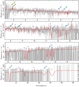
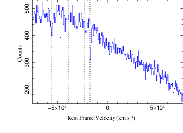
Figure 10.— Left: Results of the blind line search, utilizing 51 components. The first 24 are presented in Table 7, along with possible line IDs, presuming an outflowing wind (in the cosmological rest frame of PG 1211+143) with outflow velocity $v_{\rm out}=-17\,300~{}\rm km\,s^{-1}$ ($z_{\rm out}\sim-0.0561$). Lines labeled with question marks are those found within the first 24 components for which we have no suggested line ID. Right: Chandra 1st-order detector counts stacked in velocity bins centered on the nine identified lines in Table 7. The dashed lines are the velocities of absorber components suggested by Pounds et al. (2016a), as well as the $v_{\rm out}=-17\,300~{}\rm km\,s^{-1}$ ($z_{\rm out}=-0.0561$) absorber component discussed in this work.

Table 7Results of Blind Line Search

$\lambda_{\rm obs}$	$\lambda_{\rm rest}$	$\sigma$	$\Delta C$	$-$EW	Component	ID	$\lambda_{\rm lab}$	$z_{\rm out}$
(Å)	(Å)	(Å)		(mÅ)			(Å)	(c)
4.142	3.832	0.013	$-$11.5	$-$12.6	11	$\cdots$	$\cdots$	$\cdots$
6.173	5.830	0.002	$-$13.1	$-$6.9	6	Sixiv (Ly$\alpha$)	6.182	$-0.0586$
6.793	6.285	0.014	$-$12.4	$-$10.9	4	Sixiii (He$\alpha$)	6.648	$-0.0565$
8.219	7.603	0.009	$-$7.0	$-$7.6	21	$\cdots$	$\cdots$	$\cdots$
8.613	7.968	0.026	$-$10.9	$-$16.8	10	Mgxii (Ly$\alpha$)	8.421	$-0.0555$
8.913	8.418	0.008	$-$13.1	$-$12.8	3	$\cdots$	$\cdots$	$\cdots$
9.160	8.651	0.002	$-$9.8	$-$9.0	13	Mgxi (He$\alpha$)	9.169	$-0.0576$
10.504	9.920	0.003	$-$7.2	$-$9.8	20	$\cdots$	$\cdots$	$\cdots$
12.089	11.417	0.003	$-$9.9	22.7	19	$\cdots$	$\cdots$	$\cdots$
12.133	11.459	0.022	$-$30.0	$-$55.8	0	Nex (Ly$\alpha$)	12.133	$-0.0576$
13.453	12.705	0.013	$-$8.3	$-$31.7	16	Neix (He$\alpha$)	13.447	$-0.0565$
13.909	13.136	0.002	$-$10.1	35.7	15	$\cdots$	$\cdots$	$\cdots$
15.140	14.007	0.017	$-$13.6	$-$50.4	5	$\cdots$	$\cdots$	$\cdots$
16.338	15.430	0.009	$-$12.5	$-$52.3	9	$\cdots$	$\cdots$	$\cdots$
16.518	15.600	0.009	$-$12.5	$-$50.0	8	$\cdots$	$\cdots$	$\cdots$
16.691	15.763	0.002	$-$8.7	115.5	17	$\cdots$	$\cdots$	$\cdots$
17.739	16.753	1.132	$-$15.6	141.7	2	$\cdots$	$\cdots$	$\cdots$
18.963	17.544	0.010	$-$10.1	$-$61.2	12	Ovii (He$\beta$)	18.627	$-0.0597$
22.080	20.428	0.025	$-$7.5	$-$131.6	23	Ovii (He$\alpha$)	21.602	$-0.0555$
23.933	22.603	0.004	$-$8.2	117.5	22	$\cdots$	$\cdots$	$\cdots$
24.431	23.073	0.600	$-$22.4	$-$50.5	1	$\cdots$	$\cdots$	$\cdots$
24.855	23.473	0.129	$-$10.8	$-$354.3	14	Nvii (Ly$\alpha$)	24.781	$-0.0544$
25.584	24.161	0.130	$-$7.7	$-$437.8	18	$\cdots$	$\cdots$	$\cdots$
29.610	27.964	0.099	$-$13.2	2631.8	7	$\cdots$	$\cdots$	$\cdots$

Note. — Results from a blind search to the unbinned, combined data, using a model consisting of an absorbed disk plus powerlaw with an exponential rollover. An Fe line complex, consisting of Fe K$\alpha$/K$\beta$, Fexxv, and Fexxvi was included in all fits. The columns give: the observed wavelength and width of the line ($\lambda_{obs}$, $\sigma$), the wavelength in the PG 1211+143 cosmological rest frame, the change in Cash statistic when including the line, the line equivalent width (negative values refer to absorption), the order in which the lines were added (Component numbers 0–23), a suggested line ID, and the implied redshift in the rest frame of PG 1211+143 if this ID is correct.

Our fits indicating an outflowing wind with a velocity in the PG 1211+143 frame of $-$17 300 km s^-1 ($z_{\rm out}\sim-0.0561$) are primarily being driven by the $\alpha$ lines of Helium-like and Hydrogen-like Ne, Mg, and Si. To ensure that these lines are not being biased by our binning (although five of the six primary lines in our fits are within the uniformly binned portion of the spectrum at energies $>1$ keV), we have also performed a “blind line search” of the data. We grid the HEG data to the MEG bins, and combine all spectra, but otherwise do not perform any further channel binning. We use the same continuum model as discussed above, namely an absorbed disk plus powerlaw spectrum with exponential cutoff, and include line emission from the Fe region. We then loop through the spectra, adding one line at a time which is allowed to freely range between emission and absorption. The initial line fit is constrained to a narrow range of wavelengths (16 MEG channels, i.e., $\approx 0.18$Å), but all possible wavelength bins are searched. The line with the greatest change in fit statistic is retained. After each step, all continuum and line parameters are refit (within the constraints of the existing wavelength region of the added line). This process is repeated (51 times in Figure 10, with the first 24 found lines listed in Table 7). As the goal is to identify candidate lines, we do not calculate confidence intervals for the final lines.

The putative Ne x line is our single most significant residual, with the remaining 5 lines from H-like and He-like Ne, Mg, and Si all falling within the 17 most significant residuals. Additionally, there are three other residuals that might be associated with a $z_{\rm out}\approx-0.0561$ outflow. These, however, fall within a very low signal-to-noise region of the spectrum. Several residuals are broad, and are undoubtedly modifying the continuum fit. Several could be spurious noise features. The rest remain unidentified. However, this blind search highlights those features that are driving the xstar and warmabs models to identify an outflowing component in the rest frame of PG 1211+143.

As a further diagnostic of possible absorber components, we take the 1st-order Chandra-HETGS counts, and using the 9 potential H- and He-like lines identified in Table 7, stack the data into cosmological rest frame velocity bins. The results of this stacking are also shown in Figure 10 (note that in this procedure, not every bin is statistically independent from one another, as counts can be reused for different ions). The strong feature at a velocity in the rest frame of PG 1211+143 of $-$17 300 km s^-1 ($z_{\rm out}\sim-0.0561$) is apparent. We also indicate the velocities of the absorber components suggested by the analysis of Pounds et al. (2016a). There is a feature near the $\sim-0.19c$ ($-57\,000~{}\rm km\,s^{-1}$) velocity found by Pounds et al. (2016a), but we have not found any single line-like residual at such a velocity. It is possible, however, that such an absorption component, if real, only manifests significantly in a stacked analysis.

References

- Arnaud (1996) Arnaud, K. A. 1996, in Astronomical Society of the Pacific Conference Series, Vol. 101, Astronomical Data Analysis Software and Systems V, ed. G. H. Jacoby & J. Barnes, 17
- Bautista & Kallman (2001) Bautista, M. A. & Kallman, T. R. 2001, ApJS, 134, 139
- Bianchi et al. (2005) Bianchi, S., Matt, G., Nicastro, F., et al. 2005, MNRAS, 357, 599
- Blustin et al. (2002) Blustin, A. J., Branduardi-Raymont, G., Behar, E., et al. 2002, A&A, 392, 453
- Braito et al. (2007) Braito, V., Reeves, J. N., Dewangan, G. C., et al. 2007, ApJ, 670, 978
- Canizares et al. (2005) Canizares, C. R., Davis, J. E., Dewey, D., et al. 2005, PASP, 117, 1144
- Cappi (2006) Cappi, M. 2006, Astronomische Nachrichten, 327, 1012
- Cappi et al. (2009) Cappi, M., Tombesi, F., Bianchi, S., et al. 2009, A&A, 504, 401
- Chakravorty et al. (2009) Chakravorty, S., Kembhavi, A. K., Elvis, M., et al. 2009, MNRAS, 393, 83
- Chakravorty et al. (2013) Chakravorty, S., Lee, J. C., & Neilsen, J. 2013, MNRAS, 436, 560
- Crenshaw et al. (2003) Crenshaw, D. M., Kraemer, S. B., & George, I. M. 2003, ARA&A, 41, 117
- Danehkar et al. (2018) Danehkar, A., Nowak, M. A., Lee, J. C., et al. 2018, PASP, 130, 024501
- Danforth & Shull (2008) Danforth, C. W. & Shull, J. M. 2008, ApJ, 679, 194
- Di Matteo et al. (2005) Di Matteo, T., Springel, V., & Hernquist, L. 2005, Nature, 433, 604
- Dunn et al. (2008) Dunn, J. P., Crenshaw, D. M., Kraemer, S. B., et al. 2008, AJ, 136, 1201
- Edelson et al. (2015) Edelson, R., Gelbord, J. M., Horne, K., et al. 2015, ApJ, 806, 129
- Foreman-Mackey et al. (2013) Foreman-Mackey, D., Hogg, D. W., Lang, D., et al. 2013, PASP, 125, 306
- Foster et al. (2012) Foster, A. R., Ji, L., Smith, R. K., et al. 2012, ApJ, 756, 128
- Fruscione et al. (2006) Fruscione, A., McDowell, J. C., Allen, G. E., et al. 2006, in Proc. SPIE, Vol. 6270, Society of Photo-Optical Instrumentation Engineers (SPIE) Conference Series, 62701V
- Fukumura et al. (2010a) Fukumura, K., Kazanas, D., Contopoulos, I., et al. 2010a, ApJ, 715, 636
- Fukumura et al. (2010b) —. 2010b, ApJ, 723, L228
- Fukumura et al. (2015) Fukumura, K., Tombesi, F., Kazanas, D., et al. 2015, ApJ, 805, 17
- Gallo & Fabian (2013) Gallo, L. C. & Fabian, A. C. 2013, MNRAS, 434, L66
- Garmire et al. (2003) Garmire, G. P., Bautz, M. W., Ford, P. G., et al. 2003, in Proc. SPIE, Vol. 4851, X-Ray and Gamma-Ray Telescopes and Instruments for Astronomy., ed. J. E. Truemper & H. D. Tananbaum, 28–44
- George et al. (1998) George, I. M., Turner, T. J., Netzer, H., et al. 1998, ApJS, 114, 73
- Green et al. (2012) Green, J. C., Froning, C. S., Osterman, S., et al. 2012, ApJ, 744, 60
- Halpern (1984) Halpern, J. P. 1984, ApJ, 281, 90
- Hamann et al. (1997) Hamann, F., Barlow, T. A., Junkkarinen, V., et al. 1997, ApJ, 478, 80
- Hopkins & Elvis (2010) Hopkins, P. F. & Elvis, M. 2010, MNRAS, 401, 7
- Houck & Denicola (2000) Houck, J. C. & Denicola, L. A. 2000, in Astronomical Society of the Pacific Conference Series, Vol. 216, Astronomical Data Analysis Software and Systems IX, ed. N. Manset, C. Veillet, & D. Crabtree, 591
- Huenemoerder et al. (2011) Huenemoerder, D. P., Mitschang, A., Dewey, D., et al. 2011, AJ, 141, 129
- Kallman & Bautista (2001) Kallman, T. & Bautista, M. 2001, ApJS, 133, 221
- Kallman et al. (2009) Kallman, T. R., Bautista, M. A., Goriely, S., et al. 2009, ApJ, 701, 865
- Kallman et al. (1996) Kallman, T. R., Liedahl, D., Osterheld, A., et al. 1996, ApJ, 465, 994
- Kallman et al. (2004) Kallman, T. R., Palmeri, P., Bautista, M. A., et al. 2004, ApJS, 155, 675
- Kaspi & Behar (2006) Kaspi, S. & Behar, E. 2006, ApJ, 636, 674
- Kaspi et al. (2000) Kaspi, S., Brandt, W. N., Netzer, H., et al. 2000, ApJ, 535, L17
- Kazanas et al. (2012) Kazanas, D., Fukumura, K., Behar, E., et al. 2012, Astron. Rev., 7, 92
- Kellermann et al. (1994) Kellermann, K. I., Sramek, R. A., Schmidt, M., et al. 1994, AJ, 108, 1163
- Keyes et al. (1995) Keyes, C. D., Koratkar, A. P., Dahlem, M., et al. 1995, Faint Object Spectrograph Instrument Handbook v. 6.0 (Baltimore: STScI)
- King & Pounds (2015) King, A. & Pounds, K. 2015, ARA&A, 53, 115
- King (2010) King, A. R. 2010, MNRAS, 402, 1516
- Konigl & Kartje (1994) Konigl, A. & Kartje, J. F. 1994, ApJ, 434, 446
- Kriss et al. (2018) Kriss, G. A., Lee, J. C., Danehkar, A., et al. 2018, ApJ, 853, 166 (arXiv:1712.08850)
- Krolik & Kriss (2001) Krolik, J. H. & Kriss, G. A. 2001, ApJ, 561, 684
- Krolik et al. (1981) Krolik, J. H., McKee, C. F., & Tarter, C. B. 1981, ApJ, 249, 422
- Kubota et al. (1998) Kubota, A., Tanaka, Y., Makishima, K., et al. 1998, PASJ, 50, 667
- Laha et al. (2016) Laha, S., Guainazzi, M., Chakravorty, S., et al. 2016, MNRAS, 457, 3896
- Laha et al. (2014) Laha, S., Guainazzi, M., Dewangan, G. C., et al. 2014, MNRAS, 441, 2613
- Lee et al. (2013) Lee, J. C., Kriss, G. A., Chakravorty, S., et al. 2013, MNRAS, 430, 2650
- Lobban et al. (2016) Lobban, A. P., Pounds, K., Vaughan, S., et al. 2016, ApJ, 831, 201
- Makishima et al. (1986) Makishima, K., Maejima, Y., Mitsuda, K., et al. 1986, ApJ, 308, 635
- Marziani et al. (1996) Marziani, P., Sulentic, J. W., Dultzin-Hacyan, D., et al. 1996, ApJS, 104, 37
- Matzeu et al. (2017) Matzeu, G. A., Reeves, J. N., Braito, V., et al. 2017, MNRAS, 472, L15
- Matzeu et al. (2016) Matzeu, G. A., Reeves, J. N., Nardini, E., et al. 2016, MNRAS, 458, 1311
- McKernan et al. (2007) McKernan, B., Yaqoob, T., & Reynolds, C. S. 2007, MNRAS, 379, 1359
- Mitsuda et al. (1984) Mitsuda, K., Inoue, H., Koyama, K., et al. 1984, PASJ, 36, 741
- Nardini et al. (2015) Nardini, E., Reeves, J. N., Gofford, J., et al. 2015, Science, 347, 860
- Nicastro et al. (1999) Nicastro, F., Fiore, F., & Matt, G. 1999, ApJ, 517, 108
- Osterman et al. (2011) Osterman, S., Green, J., Froning, C., et al. 2011, Ap&SS, 335, 257
- Palmeri et al. (2003) Palmeri, P., Mendoza, C., Kallman, T. R., et al. 2003, A&A, 410, 359
- Parker et al. (2017a) Parker, M. L., Alston, W. N., Buisson, D. J. K., et al. 2017a, MNRAS, 469, 1553
- Parker et al. (2017b) Parker, M. L., Pinto, C., Fabian, A. C., et al. 2017b, Nature, 543, 83
- Penton et al. (2004) Penton, S. V., Stocke, J. T., & Shull, J. M. 2004, ApJS, 152, 29
- Peterson et al. (2004) Peterson, B. M., Ferrarese, L., Gilbert, K. M., et al. 2004, ApJ, 613, 682
- Petric et al. (2015) Petric, A. O., Ho, L. C., Flagey, N. J. M., et al. 2015, ApJS, 219, 22
- Pinto et al. (2017) Pinto, C., Alston, W., Soria, R., et al. 2017, MNRAS, 468, 2865
- Pounds et al. (2016a) Pounds, K., Lobban, A., Reeves, J., et al. 2016a, MNRAS, 457, 2951
- Pounds (2014) Pounds, K. A. 2014, MNRAS, 437, 3221
- Pounds et al. (2016b) Pounds, K. A., Lobban, A., Reeves, J. N., et al. 2016b, MNRAS, 459, 4389
- Pounds & Page (2006) Pounds, K. A. & Page, K. L. 2006, MNRAS, 372, 1275
- Pounds & Reeves (2007) Pounds, K. A. & Reeves, J. N. 2007, MNRAS, 374, 823
- Pounds & Reeves (2009) —. 2009, MNRAS, 397, 249
- Pounds et al. (2003) Pounds, K. A., Reeves, J. N., King, A. R., et al. 2003, MNRAS, 345, 705
- Proga (2003) Proga, D. 2003, ApJ, 585, 406
- Proga et al. (2000) Proga, D., Stone, J. M., & Kallman, T. R. 2000, ApJ, 543, 686
- Reeves et al. (2018) Reeves, J., Lobban, A., & Pounds, K. 2018, ApJ, in press (arXiv:1801.03784)
- Reeves & Pounds (2012) Reeves, J. & Pounds, K. 2012, in Astronomical Society of the Pacific Conference Series, Vol. 460, AGN Winds in Charleston, ed. G. Chartas, F. Hamann, & K. M. Leighly, 13
- Reeves et al. (2016) Reeves, J. N., Braito, V., Nardini, E., et al. 2016, ApJ, 824, 20
- Reeves et al. (2005) Reeves, J. N., Pounds, K., Uttley, P., et al. 2005, ApJ, 633, L81
- Reynolds (1997) Reynolds, C. S. 1997, MNRAS, 286, 513
- Reynolds & Fabian (1995) Reynolds, C. S. & Fabian, A. C. 1995, MNRAS, 273, 1167
- Rines et al. (2003) Rines, K., Geller, M. J., Kurtz, M. J., et al. 2003, AJ, 126, 2152
- Schlafly & Finkbeiner (2011) Schlafly, E. F. & Finkbeiner, D. P. 2011, ApJ, 737, 103
- Smith et al. (2016) Smith, R. K., Abraham, M. H., Allured, R., et al. 2016, in Proc. SPIE, Vol. 9905, Space Telescopes and Instrumentation 2016: Ultraviolet to Gamma Ray, 99054M
- Spitzer (1978) Spitzer, L. 1978, Physical processes in the interstellar medium (New York: Wiley-Interscience)
- Tarter et al. (1969) Tarter, C. B., Tucker, W. H., & Salpeter, E. E. 1969, ApJ, 156, 943
- Tilton et al. (2012) Tilton, E. M., Danforth, C. W., Shull, J. M., et al. 2012, ApJ, 759, 112
- Tombesi et al. (2012) Tombesi, F., Cappi, M., Reeves, J. N., et al. 2012, MNRAS, 422, 1
- Tombesi et al. (2013) —. 2013, MNRAS, 430, 1102
- Tombesi et al. (2011) —. 2011, ApJ, 742, 44
- Tombesi et al. (2010) —. 2010, A&A, 521, A57
- Tombesi et al. (2014) Tombesi, F., Tazaki, F., Mushotzky, R. F., et al. 2014, MNRAS, 443, 2154
- Tumlinson et al. (2005) Tumlinson, J., Shull, J. M., Giroux, M. L., et al. 2005, ApJ, 620, 95
- Wakker et al. (2011) Wakker, B. P., Lockman, F. J., & Brown, J. M. 2011, ApJ, 728, 159
- Weisskopf et al. (2002) Weisskopf, M. C., Brinkman, B., Canizares, C., et al. 2002, PASP, 114, 1
- Wilms et al. (2000) Wilms, J., Allen, A., & McCray, R. 2000, ApJ, 542, 914
- Zoghbi et al. (2015) Zoghbi, A., Miller, J. M., Walton, D. J., et al. 2015, ApJ, 799, L24