EUROPEAN ORGANIZATION FOR NUCLEAR RESEARCH (CERN)

​​​ CERN-EP-2017-315 LHCb-PAPER-2017-047 December 20, 2017

Measurement of $C\!P$ asymmetry in ${{B}^{0}_{s}}\!\rightarrow D_{s}^{\mp}K^{\pm}$ decays

LHCb collaboration

We report the measurements of the $C\!P$-violating parameters in ${{B}^{0}_{s}}\!\rightarrow D_{s}^{\mp}K^{\pm}$ decays observed in $pp$ collisions, using a data set corresponding to an integrated luminosity of 3.0$\mbox{\,fb}^{-1}$ recorded with the LHCb detector. We measure $C_{f}=0.73\pm 0.14\pm 0.05$, ${A_{f}^{\Delta\Gamma}}=0.39\pm 0.28\pm 0.15$, ${A_{\overline{f}}^{\Delta\Gamma}}=0.31\pm 0.28\pm 0.15$, $S_{f}=-0.52\pm 0.20\pm 0.07$, $S_{\overline{f}}=-0.49\pm 0.20\pm 0.07$, where the uncertainties are statistical and systematic, respectively. These parameters are used together with the world-average value of the ${{B}^{0}_{s}}$ mixing phase, $-2\beta_{s}$, to obtain a measurement of the CKM angle $\gamma$ from ${{B}^{0}_{s}}\!\rightarrow D_{s}^{\mp}K^{\pm}$ decays, yielding $\gamma=(128\,_{-22}^{+17})^{\circ}$ modulo $180^{\circ}$, where the uncertainty contains both statistical and systematic contributions. This corresponds to $3.8\,\sigma$ evidence for $C\!P$ violation in the interference between decay and decay after mixing.

Published in JHEP 03 (2018) 059

© CERN on behalf of the LHCb collaboration, licence CC-BY-4.0.

 

1 Introduction

A key characteristic of the Standard Model (SM) is that $C\!P$ violation originates from a single phase in the CKM quark-mixing matrix [1, 2]. In the SM the CKM matrix is unitary, leading to the condition $V_{ud}^{\phantom{*}}V_{ub}^{*}+V_{cd}^{\phantom{*}}V_{cb}^{*}+V_{td}^{\phantom{*}}V_{tb}=0$, where $V_{ij}$ are the CKM matrix elements. This relation is represented as a triangle in the complex plane, with angles $\alpha$, $\beta$ and $\gamma$, and an area proportional to the amount of $C\!P$ violation in the quark sector of the SM [3, 4, 5]. The angle $\gamma\equiv\arg(-V^{\phantom{*}}_{ud}V_{ub}^{*}/V^{\phantom{*}}_{cd}V_{cb}^{*})$ is the least well-known angle of the CKM angles. Its current best determination was obtained by LHCb from a combination of measurements concerning ${{B}^{+}}$, ${B}^{0}$ and ${B}^{0}_{s}$ decays to final states with a $D_{(s)}$ meson and one or more light mesons[6]. Decay-time-dependent analyses of tree-level ${B}^{0}_{(s)}\rightarrow{D}^{\mp}_{(s)}{h^{\pm}}$ ($h=\pi,K$) decays are sensitive to the angle $\gamma$ through $C\!P$ violation in the interference of mixing and decay amplitudes [7, 8, 9, 10]. A comparison between the value of the CKM angle $\gamma$ obtained from tree-level processes, with the measurements of $\gamma$ and other unitary triangle parameters in loop-level processes, provides a powerful consistency check of the SM picture of $C\!P$ violation.

Due to the interference between mixing and decay amplitudes, the physical $C\!P$-violating parameters in these decays are functions of a combination of the angle $\gamma$ and the relevant mixing phase, namely $\gamma+2\beta$ ($\beta\equiv\arg(-V^{\phantom{*}}_{cd}V_{cb}^{*}/V^{\phantom{*}}_{td}V_{tb}^{*})$) in the ${B}^{0}$ and $\gamma-2\beta_{s}$ ($\beta_{s}\equiv\arg(-V^{\phantom{*}}_{ts}V_{tb}^{*}/V^{\phantom{*}}_{cs}V_{cb}^{*})$) in the ${B}^{0}_{s}$ system. Measurements of these physical quantities can therefore be interpreted in terms of the angles $\gamma$ or $\beta_{(s)}$ by using independent determinations of the other parameter as input. Such measurements have been performed by both the BaBar [11, 12] and Belle [13, 14] collaborations using ${{B}^{0}}\rightarrow D^{(*)\mp}\pi^{\pm}$ decays. In these decays, the ratios between the interfering $b\rightarrow u$ and $b\rightarrow c$ amplitudes are small, $r_{D^{(*)}\pi}=|A({{B}^{0}}\rightarrow D^{(*)-}\pi^{+})/A({{B}^{0}}\rightarrow D^{(*)+}\pi^{-})|\approx 0.02$, which limits the sensitivity to the CKM angle $\gamma$ [15].

The leading-order Feynman diagrams contributing to the interference of decay and mixing in ${{B}^{0}_{s}}\!\rightarrow D_{s}^{\mp}K^{\pm}$ decays are shown in Fig. 1. In contrast to ${{B}^{0}}\rightarrow D^{(*)\mp}\pi^{\pm}$ decays, here both the ${{B}^{0}_{s}}\!\rightarrow D_{s}^{-}K^{+}$ ($b\rightarrow cs\bar{u}$) and the ${{B}^{0}_{s}}\!\rightarrow D_{s}^{+}K^{-}$ ($b\rightarrow u\bar{c}s$) decay amplitudes are of $\mathcal{O}(\lambda^{3})$, where $\lambda\approx 0.23$ [16, 17] is the sine of the Cabibbo angle, and the ratio of the amplitudes of the interfering diagrams is approximately $|V_{ub}^{*}V^{\phantom{*}}_{cs}/V^{\phantom{*}}_{cb}V_{us}^{*}|\approx 0.4$. Moreover, the sizeable decay-width difference in the ${B}^{0}_{s}$ system, $\Delta\Gamma_{s}$ [18], allows the determination of $\gamma-2\beta_{s}$ from the sinusoidal and hyperbolic terms of the decay-time evolution (see Eqs. 1 and 2) up to a two-fold ambiguity.

This paper presents an updated measurement with respect to Ref. [19] of the $C\!P$-violating parameters and of $\gamma-2\beta_{s}$ in ${{B}^{0}_{s}}\!\rightarrow D_{s}^{\mp}K^{\pm}$ decays using a data set corresponding to an integrated luminosity of 1.0 (2.0) $\mbox{\,fb}^{-1}$ of $pp$ collisions recorded with the LHCb detector at $\sqrt{s}=7\,(8)\mathrm{\,Te\kern-1.00006ptV}$ in 2011 (2012).

   

Figure 1: Feynman diagrams for ${{\kern 1.79993pt\overline{\kern-1.79993ptB}{}}{}^{0}_{s}}\!\rightarrow D_{s}^{+}K^{-}$ decays (left) without and (right) with ${B}^{0}_{s}$–${\kern 1.79993pt\overline{\kern-1.79993ptB}{}}{}^{0}_{s}$ mixing.

1.1 Decay rate equations and $C\!P$ violation parameters

The time-dependent-decay rates of the initially produced flavour eigenstates $|{{B}^{0}_{s}}(t=0)\rangle$ and $|{{\kern 1.79993pt\overline{\kern-1.79993ptB}{}}{}^{0}_{s}}(t=0)\rangle$ are given by

$$\frac{{\rm d}\Gamma_{{{B}^{0}_{s}}\rightarrow f}(t)}{{\rm d}t} =\frac{1}{2}|A_{f}|^{2}(1+|\lambda_{f}|^{2})e^{-\Gamma_{s}t}\left[\cosh\left(\frac{\Delta\Gamma_{s}t}{2}\right)+{A_{f}^{\Delta\Gamma}}\sinh\left(\frac{\Delta\Gamma_{s}t}{2}\right)\right.$$

$$+C_{f}\cos\left(\Delta m_{s}t\right)-S_{f}\sin\left(\Delta m_{s}t\right)\Big{]},$$ (1)

$$\frac{{\rm d}\Gamma_{{{\kern 1.25995pt\overline{\kern-1.25995ptB}{}}{}^{0}_{s}}\rightarrow f}(t)}{{\rm d}t} =\frac{1}{2}|A_{f}|^{2}\left|\frac{p}{q}\right|^{2}(1+|\lambda_{f}|^{2})e^{-\Gamma_{s}t}\left[\cosh\left(\frac{\Delta\Gamma_{s}t}{2}\right)+{A_{f}^{\Delta\Gamma}}\sinh\left(\frac{\Delta\Gamma_{s}t}{2}\right)\right.$$

$$-C_{f}\cos\left(\Delta m_{s}t\right)+S_{f}\sin\left(\Delta m_{s}t\right)\Big{]},$$ (2)

where $\lambda_{f}\equiv(q/p)(\overline{A}_{f}/A_{f})$ and $A_{f}$ ($\overline{A}_{f}$) is the amplitude of a ${B}^{0}_{s}$ (${\kern 1.79993pt\overline{\kern-1.79993ptB}{}}{}^{0}_{s}$) decay to the final state $f$, $\Gamma_{s}$ corresponds to the average ${B}^{0}_{s}$ decay width, while $\Delta\Gamma_{s}$ indicates the decay-width difference between the light, $|B_{L}\rangle$, and heavy, $|B_{H}\rangle$, ${B}^{0}_{s}$ mass eigenstates, defined as $\Gamma_{B_{L}}-\Gamma_{B_{H}}$ and $\Delta m_{s}$ is the mixing frequency in the ${B}^{0}_{s}$ system defined as $m_{B_{H}}-m_{B_{L}}$. The complex coefficients $p$ and $q$ relate the ${B}^{0}_{s}$ meson mass eigenstates, to the flavour eigenstates, where

$$|B_{L}\rangle=p|{{B}^{0}_{s}}\rangle+q|{{\kern 1.79993pt\overline{\kern-1.79993ptB}{}}{}^{0}_{s}}\rangle\;\;\;{\text{and}}\;\;\;|B_{H}\rangle=p|{{B}^{0}_{s}}\rangle-q|{{\kern 1.79993pt\overline{\kern-1.79993ptB}{}}{}^{0}_{s}}\rangle\,,$$ (3)

with $|p|^{2}+|q|^{2}=1$. Equations similar to 1 and 2 can be written for the decays to the $C\!P$-conjugate final state $\overline{f}$ replacing $C_{f}$ by $C_{\overline{f}}$, $S_{f}$ by $S_{\overline{f}}$, and ${A_{f}^{\Delta\Gamma}}$ by ${A_{\overline{f}}^{\Delta\Gamma}}$. In what follows, the convention that $f$ ($\overline{f}$) indicates ${{D}^{-}_{s}}{{K}^{+}}$ (${{D}^{+}_{s}}{{K}^{-}}$) final state is used. The $C\!P$-asymmetry parameters are given by

$$C_{f}=\frac{1-|\lambda_{f}|^{2}}{1+|\lambda_{f}|^{2}} =-C_{\overline{f}}=-\frac{1-|\lambda_{\overline{f}}|^{2}}{1+|\lambda_{\overline{f}}|^{2}}\,,$$ (4)

$$S_{f}=\frac{2\mathcal{I}m(\lambda_{f})}{1+|\lambda_{f}|^{2}} ,\quad{A_{f}^{\Delta\Gamma}}=\frac{-2\mathcal{R}e(\lambda_{f})}{1+|\lambda_{f}|^{2}}\,,$$

$$S_{\overline{f}}=\frac{2\mathcal{I}m(\lambda_{\overline{f}})}{1+|\lambda_{\overline{f}}|^{2}} ,\quad{A_{\overline{f}}^{\Delta\Gamma}}=\frac{-2\mathcal{R}e(\lambda_{\overline{f}})}{1+|\lambda_{\overline{f}}|^{2}}\,.$$

The equality $C_{f}=-C_{\overline{f}}$ results from $|q/p|=1$ and $|\lambda_{f}|=|1/\lambda_{\overline{f}}|$, i.e. assuming no $C\!P$ violation in either the mixing, in agreement with current measurements [20], or in the decay amplitude, which is justified as only a single amplitude contributes to each initial to final state transition. The $C\!P$ parameters are related to the magnitude of the amplitude ratio $r_{D_{s}K}\equiv|\lambda_{D_{s}K}|=|A({{\kern 1.79993pt\overline{\kern-1.79993ptB}{}}{}^{0}_{s}}\rightarrow{{D}^{-}_{s}}{{K}^{+}})/A({{B}^{0}_{s}}\rightarrow{{D}^{-}_{s}}{{K}^{+}})|$, the strong-phase difference $\delta$ between the amplitudes $A({{\kern 1.79993pt\overline{\kern-1.79993ptB}{}}{}^{0}_{s}}\rightarrow{{D}^{-}_{s}}{{K}^{+}})$ and $A({{B}^{0}_{s}}\rightarrow{{D}^{-}_{s}}{{K}^{+}})$, and the weak-phase difference $\gamma-2\beta_{s}$ by the following equations

$$C_{f}= \frac{1-r_{D_{s}K}^{2}}{1+r_{D_{s}K}^{2}}\,,$$ (5)

$${A_{f}^{\Delta\Gamma}}=\frac{-2r_{D_{s}K}\cos(\delta-(\gamma-2\beta_{s}))}{1+r_{D_{s}K}^{2}} ,\quad{A_{\overline{f}}^{\Delta\Gamma}}=\frac{-2r_{D_{s}K}\cos(\delta+(\gamma-2\beta_{s}))}{1+r_{D_{s}K}^{2}}\,,$$

$$S_{f}=\frac{2r_{D_{s}K}\sin(\delta-(\gamma-2\beta_{s}))}{1+r_{D_{s}K}^{2}} ,\quad S_{\overline{f}}=\frac{-2r_{D_{s}K}\sin(\delta+(\gamma-2\beta_{s}))}{1+r_{D_{s}K}^{2}}\,.$$

1.2 Analysis strategy

The analysis strategy consists of a two-stage procedure. After the event selection, an unbinned extended maximum likelihood fit, referred to as the multivariate fit, is performed to separate signal ${{B}^{0}_{s}}\!\rightarrow D_{s}^{\mp}K^{\pm}$ candidates from background contributions. The multivariate fit uses the ${B}^{0}_{s}$ and ${D}^{-}_{s}$ invariant masses and the log-likelihood difference between the pion and kaon hypotheses, $L(K/\pi)$, for the $K^{\pm}$ candidate. Using information from this fit, signal weights for each candidate are obtained using the sPlot technique [21]. At the second stage, the $C\!P$ violation parameters are measured from a fit to the weighted decay-time distribution, referred to as the sFit [22] procedure, where the initial flavour of the ${B}^{0}_{s}$ candidate is inferred by means of several flavour-tagging algorithms optimised using data and simulation samples. The full procedure is validated using the flavour-specific ${{B}^{0}_{s}}\!\rightarrow{{D}^{-}_{s}}{{\pi}^{+}}$ decay, yielding approximately 16 times more signal than ${{B}^{0}_{s}}\!\rightarrow D_{s}^{\mp}K^{\pm}$ decays. Precise determination of the decay-time resolution model and of the decay-time acceptance, as well as the calibration of the flavour-tagging algorithms, are obtained from ${{B}^{0}_{s}}\!\rightarrow{{D}^{-}_{s}}{{\pi}^{+}}$ decays and subsequently used in the sFit procedure to the ${{B}^{0}_{s}}\!\rightarrow D_{s}^{\mp}K^{\pm}$ candidates. The analysis strategy largely follows that described in Ref. [19]. Most of the inputs are updated, in particular the candidate selection, the flavour tagging calibration and the decay-time resolution are optimised on the current data and simulation samples. A more refined estimate of the systematic uncertainties is also performed. After a brief description of the LHCb detector in Sec. 2, the event selection is reported in Sec. 3. The relevant inputs for the multivariate fit and its results for ${{B}^{0}_{s}}\!\rightarrow D_{s}^{\mp}K^{\pm}$ and ${{B}^{0}_{s}}\!\rightarrow{{D}^{-}_{s}}{{\pi}^{+}}$ decays are outlined in Secs. 4. The flavour-tagging parameters and the decay-time resolution model are described in Secs. 5 and 6, respectively. The decay-time acceptance is reported in Sec. 7 followed by the results of the sFit procedure applied to ${{B}^{0}_{s}}\!\rightarrow D_{s}^{\mp}K^{\pm}$ candidates in Sec. 8. The evaluation of the systematic uncertainties and the interpretation for the CKM angle $\gamma$ are summarised in Secs. 9 and 10, respectively. Conclusions are drawn in Sec. 11.

2 Detector and software

The LHCb detector [23, 24] is a single-arm forward spectrometer covering the pseudorapidity range $2<\eta<5$, designed for the study of particles containing $b$ or $c$ quarks. The detector includes a high-precision tracking system consisting of a silicon-strip vertex detector surrounding the $pp$ interaction region [25], a large-area silicon-strip detector located upstream of a dipole magnet with a bending power of about $4{\mathrm{\,Tm}}$, and three stations of silicon-strip detectors and straw drift tubes [26] placed downstream of the magnet. The polarity of the dipole magnet is reversed periodically throughout data taking to control systematic effects. The tracking system provides a measurement of momentum, $p$, of charged particles with a relative uncertainty that varies from 0.5% at low momentum to 1.0% at 200${\mathrm{\,Ge\kern-1.00006ptV\!/}c}$. The minimum distance of a track to a primary vertex (PV), the impact parameter (IP), is measured with a resolution of $(15+29/\mbox{$p_{\mathrm{T}}$}){\,\upmu\mathrm{m}}$, where $p_{\mathrm{T}}$ is the component of the momentum transverse to the beam, in ${\mathrm{\,Ge\kern-1.00006ptV\!/}c}$. Particle identification (PID) of charged hadrons is achieved using information from two ring-imaging Cherenkov detectors [27].

The online event selection is performed by a trigger [28], which consists of a hardware stage, based on information from the calorimeters and muon systems, followed by a software stage, which applies a full event reconstruction. At the hardware trigger stage, events are required to have a muon with high $p_{\mathrm{T}}$ or a hadron, photon or electron with high transverse energy in the calorimeters. For hadrons, the transverse energy threshold is 3.5$\mathrm{\,Ge\kern-1.00006ptV}$. The software trigger requires a two-, three- or four-track secondary vertex with a significant displacement from any primary $pp$ interaction vertex. At least one charged particle must have a transverse momentum $\mbox{$p_{\mathrm{T}}$}>1.6{\mathrm{\,Ge\kern-1.00006ptV\!/}c}$ and be inconsistent with originating from any PV. A multivariate algorithm [29] is used for the identification of secondary vertices consistent with the decay of a $b$ hadron.

In the simulation, $pp$ collisions are generated using Pythia [30, 31] with a specific LHCb configuration [32]. Decays of hadronic particles are described by EvtGen [33], in which final-state radiation is generated using Photos [34]. The interaction of the generated particles with the detector, and its response, are implemented using the Geant4 toolkit [35, *Agostinelli:2002hh] as described in Ref. [37].

3 Candidate selection

First, ${{D}^{-}_{s}}\!\rightarrow{{K}^{-}}{{K}^{+}}{{\pi}^{-}}$, ${{D}^{-}_{s}}\!\rightarrow{{K}^{-}}{{\pi}^{+}}{{\pi}^{-}}$, and ${{D}^{-}_{s}}\!\rightarrow{{\pi}^{-}}{{\pi}^{+}}{{\pi}^{-}}$ candidates are formed from reconstructed charged particles. These ${D}^{-}_{s}$ candidates are subsequently combined with a fourth particle, referred to as the “companion”, to form ${{B}^{0}_{s}}\!\rightarrow D_{s}^{\mp}K^{\pm}$ or ${{B}^{0}_{s}}\!\rightarrow{{D}^{-}_{s}}{{\pi}^{+}}$ candidates, depending on the PID information of the companion particle. The decay-time resolution is improved by performing a kinematic fit [38] in which the ${B}^{0}_{s}$ candidate is assigned to a PV for which it has the smallest impact parameter $\chi^{2}$, defined as the difference in the $\chi^{2}$ of the vertex fit for a given PV reconstructed with and without the considered particle. Similarly, the ${B}^{0}_{s}$ invariant mass resolution is improved by constraining the ${D}^{-}_{s}$ invariant mass to its world-average value.

A selection of reconstructed candidates is made using a similar multivariate secondary-vertex algorithm as that applied at the trigger level, but with offline-quality reconstruction [29]. Combinatorial background is further suppressed by a gradient boosted decision tree (BDTG) algorithm [39, 40], which is trained on ${{B}^{0}_{s}}\!\rightarrow{{D}^{-}_{s}}{{\pi}^{+}}$ data. Only the ${{D}^{-}_{s}}\!\rightarrow{{K}^{-}}{{K}^{+}}{{\pi}^{-}}$ final state selected with additional PID requirements is considered in order to enrich the training sample with signal candidates. Since all channels in this analysis have similar kinematics, and no PID information is used as input to the BDTG, the resulting BDTG performs equally well on the other ${D}^{-}_{s}$ decay modes. The optimal working point is chosen to maximise the significance of the ${{B}^{0}_{s}}\!\rightarrow D_{s}^{\mp}K^{\pm}$ signal. In addition, the ${B}^{0}_{s}$ and ${D}^{-}_{s}$ candidates are required to have a measured mass within $[5300,5800]{\mathrm{\,Me\kern-1.00006ptV\!/}c^{2}}$ and $[1930,2015]{\mathrm{\,Me\kern-1.00006ptV\!/}c^{2}}$, respectively.

Finally, a combination of PID information and kinematic vetoes is used to distinguish the different ${D}^{-}_{s}$ final states from each other (${{D}^{-}_{s}}\!\rightarrow{{K}^{-}}{{\pi}^{+}}{{\pi}^{-}}$, ${{D}^{-}_{s}}\!\rightarrow{{\pi}^{-}}{{\pi}^{+}}{{\pi}^{-}}$ and ${{D}^{-}_{s}}\!\rightarrow{{K}^{-}}{{K}^{+}}{{\pi}^{-}}$, the latter being subdivided into ${{D}^{-}_{s}}\!\rightarrow\phi{{\pi}^{-}}$, ${{D}^{-}_{s}}\rightarrow K^{*}(892)^{0}{{K}^{-}}$ and ${{D}^{-}_{s}}\!\rightarrow(KK\pi)_{\rm nonres}$) and from cross-feed backgrounds such as ${{B}^{0}}\!\rightarrow{{D}^{-}}{{K}^{+}}$ or ${{\kern 1.00006pt\overline{\kern-1.00006pt\mathchar 28931\relax}}{}^{0}_{b}}\!\rightarrow{{\kern 1.00006pt\overline{\kern-1.00006pt\mathchar 28931\relax}}{}^{-}_{c}}{{K}^{+}}$ decays. The selection structure and most criteria are identical to those used in Ref. [19]; the specific values of certain PID selection requirements were updated to perform optimally with the latest event reconstruction algorithms. Less than 1% of the events passing the selection requirements contain more than one signal candidate. All candidates are used in the analysis.

4 Multivariate fit to ${{B}^{0}_{s}}\!\rightarrow D_{s}^{\mp}K^{\pm}$ and ${{B}^{0}_{s}}\!\rightarrow{{D}^{-}_{s}}{{\pi}^{+}}$

The signal and background probability density functions (PDFs) for the multivariate fit are obtained using a mixture of data-driven approaches and simulation. The simulated events are corrected for differences in the transverse momentum and event occupancy distributions between simulation and data, as well as for the kinematics-dependent efficiency of the PID selection requirements.

The shape of the ${B}^{0}_{s}$ invariant mass distribution for signal candidates is modelled using the sum of two Crystal Ball functions with a common mean [41]. This choice of functions provides a good description of the main peak as well as the radiative tail and reconstruction effects. The signal PDFs are determined separately for the ${{B}^{0}_{s}}\!\rightarrow D_{s}^{\mp}K^{\pm}$ and ${{B}^{0}_{s}}\!\rightarrow{{D}^{-}_{s}}{{\pi}^{+}}$ decays from simulation, taking into account different ${D}^{-}_{s}$ final states. The shapes are fixed in the nominal fit with two exceptions. The common mean of the Crystal Ball functions is left free for both ${{B}^{0}_{s}}\!\rightarrow{{D}^{-}_{s}}{{\pi}^{+}}$ and ${{B}^{0}_{s}}\!\rightarrow D_{s}^{\mp}K^{\pm}$, compensating for differences in the mass reconstruction between simulation and data. A scale factor accounting for data-simulation differences in the signal width is left free in the ${{B}^{0}_{s}}\!\rightarrow{{D}^{-}_{s}}{{\pi}^{+}}$ fit and is subsequently fixed to its measured value in the fit to the ${{B}^{0}_{s}}\!\rightarrow D_{s}^{\mp}K^{\pm}$ sample.

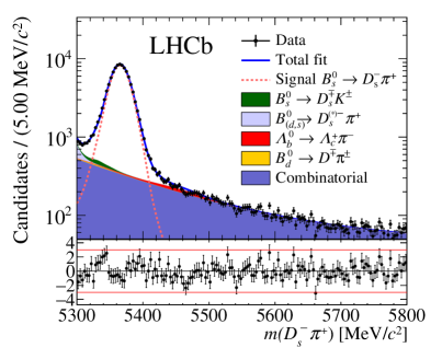
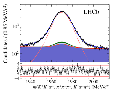
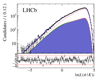
Figure 2: Distributions of the (upper left) ${B}^{0}_{s}$ and (upper right) ${D}^{-}_{s}$ invariant masses for ${{B}^{0}_{s}}\!\rightarrow{{D}^{-}_{s}}{{\pi}^{+}}$ final states, and (bottom) of the logarithm of the companion track PID log-likelihood, $\ln(L(\pi/K))$. In each plot, the contributions from all ${D}^{-}_{s}$ final states are combined. The solid blue curve is the total result of the simultaneous fit. The dotted red curve shows the ${{B}^{0}_{s}}\!\rightarrow{{D}^{-}_{s}}{{\pi}^{+}}$ signal and the fully coloured stacked histograms show the different background contributions. Normalised residuals are shown underneath all distributions.

The functional form of the combinatorial background is taken from the ${B}^{0}_{s}$ invariant mass sideband (above $5800{\mathrm{\,Me\kern-1.00006ptV\!/}c^{2}}$), with all parameters left free to vary in the multivariate fit. It is parametrised separately for each ${D}^{-}_{s}$ mode either by an exponential function or by the sum of an exponential function and a constant offset. The shapes of the fully or partially reconstructed backgrounds are fixed from simulated events, corrected to reproduce the PID efficiency and kinematics in data, using a nonparametric kernel estimation method (KEYS) [42]. An exception is background due to ${B}^{0}$ mesons decaying to the same final state as signal, which is parametrised by the signal PDF shifted by the known ${B}^{0}$–${B}^{0}_{s}$ mass difference.

The ${D}^{-}_{s}$ invariant mass is also described by a sum of two Crystal Ball functions with a common mean. The signal PDFs are obtained from simulation separately for each ${D}^{-}_{s}$ decay mode. As for the ${B}^{0}_{s}$ invariant mass signal shape, only the common mean and the width scale factor are left free in the fits; the ${B}^{0}_{s}$ and ${D}^{-}_{s}$ scale factors are different. The combinatorial background consists of random combinations of tracks that do not originate from a ${D}^{-}_{s}$ meson decay and backgrounds that contain a true ${D}^{-}_{s}$ decay combined with a random companion track. Its shape is parametrised, separately for each ${D}^{-}_{s}$ decay mode, by a combination of an exponential function and the corresponding ${D}^{-}_{s}$ signal PDF. The fully and partially reconstructed backgrounds that contain a correctly reconstructed ${D}^{-}_{s}$ candidate (${{B}^{0}_{s}}\!\rightarrow D_{s}^{\mp}K^{\pm}$ and ${{B}^{0}}\!\rightarrow{{D}^{-}_{s}}{{\pi}^{+}}$ as backgrounds in the ${{B}^{0}_{s}}\!\rightarrow{{D}^{-}_{s}}{{\pi}^{+}}$ fit; ${{B}^{0}}\!\rightarrow{{D}^{-}_{s}}{{K}^{+}}$, ${{B}^{0}_{s}}\!\rightarrow{{D}^{*-}_{s}}{{\pi}^{+}}$, ${{B}^{0}_{s}}\!\rightarrow{{D}^{-}_{s}}\rho^{+}$ and ${{B}^{0}_{s}}\!\rightarrow{{D}^{-}_{s}}{{\pi}^{+}}$ as backgrounds in the ${{B}^{0}_{s}}\!\rightarrow D_{s}^{\mp}K^{\pm}$ fit) are assumed to have the same ${D}^{-}_{s}$ invariant mass distribution as the signal. The shapes of the other backgrounds are KEYS templates taken from simulation.

The PDFs describing the $L(K/\pi)$ distributions of pions, kaons and protons are obtained from dedicated data-driven calibration samples [43].

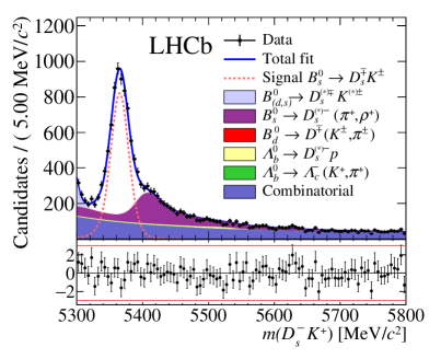
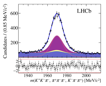
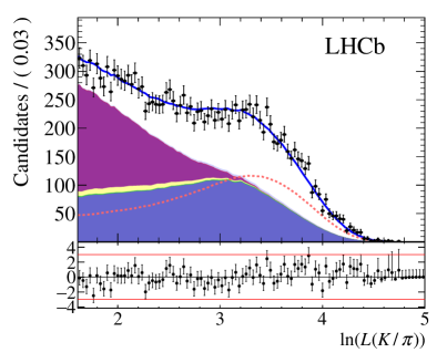
Figure 3: Distributions of the (upper left) ${B}^{0}_{s}$ and (upper right) ${D}^{-}_{s}$ invariant masses for ${{B}^{0}_{s}}\!\rightarrow D_{s}^{\mp}K^{\pm}$ final states, and (bottom) of the logarithm of the companion track PID log-likelihood, $\ln(L(K/\pi))$. In each plot, the contributions from all ${D}^{-}_{s}$ final states are combined. The solid blue curve is the total result of the simultaneous fit. The dotted red curve shows the ${{B}^{0}_{s}}\!\rightarrow{{D}^{-}_{s}}{{\pi}^{+}}$ signal and the fully coloured stacked histograms show the different background contributions. Normalised residuals are shown underneath all distributions.

The $L(K/\pi)$ shape of the companion track for the signal is obtained separately for each ${D}^{-}_{s}$ decay mode to account for small kinematic differences between them. For the combinatorial background, the $L(K/\pi)$ PDF is determined from a mixture of pion, proton, and kaon contributions, and its normalisation is left free in the multivariate fit. For fully or partially reconstructed backgrounds the $L(K/\pi)$ PDF is obtained by weighting the PID calibration samples to match the event distributions of simulated events, separately for each background type.

The multivariate fit is performed simultaneously to the different ${D}^{-}_{s}$ decay modes. For each ${D}^{-}_{s}$ decay mode the PDF is built from the sum of signal and background contributions. Each contribution consists of the product of three PDFs corresponding to the ${B}^{0}_{s}$ and $D_{s}$ invariant masses and $L(K/\pi)$, since their correlations are measured to be small in simulation. A systematic uncertainty is assigned to account for the impact of residual correlations.

Almost all background yields are left free to vary in the fit, except those that have an expected contribution below 2% of the signal yield, namely: ${{B}^{0}}\!\rightarrow{{D}^{-}}{{K}^{+}}$, ${{B}^{0}}\!\rightarrow{{D}^{-}}{{\pi}^{+}}$, ${{\kern 1.00006pt\overline{\kern-1.00006pt\mathchar 28931\relax}}{}^{0}_{b}}\!\rightarrow{{\kern 1.00006pt\overline{\kern-1.00006pt\mathchar 28931\relax}}{}^{-}_{c}}{{K}^{+}}$, and ${{\kern 1.00006pt\overline{\kern-1.00006pt\mathchar 28931\relax}}{}^{0}_{b}}\!\rightarrow{{\kern 1.00006pt\overline{\kern-1.00006pt\mathchar 28931\relax}}{}^{-}_{c}}{{\pi}^{+}}$ for the ${{B}^{0}_{s}}\!\rightarrow D_{s}^{\mp}K^{\pm}$ fit, and ${{B}^{0}}\!\rightarrow{{D}^{-}}{{\pi}^{+}}$, ${{\kern 1.00006pt\overline{\kern-1.00006pt\mathchar 28931\relax}}{}^{0}_{b}}\!\rightarrow{{\kern 1.00006pt\overline{\kern-1.00006pt\mathchar 28931\relax}}{}^{-}_{c}}{{\pi}^{+}}$, and ${{B}^{0}_{s}}\!\rightarrow D_{s}^{\mp}K^{\pm}$ for the ${{B}^{0}_{s}}\!\rightarrow{{D}^{-}_{s}}{{\pi}^{+}}$ fit. Such background yields are fixed from known branching fractions and relative efficiencies measured using simulation.

The multivariate fit results in total signal yields of $96\ 942\pm 345$ and $5955\pm 90$ ${{B}^{0}_{s}}\!\rightarrow{{D}^{-}_{s}}{{\pi}^{+}}$ and ${{B}^{0}_{s}}\!\rightarrow D_{s}^{\mp}K^{\pm}$ signal candidates, respectively. Signal yields are increased by a factor of 3.4 with respect to the previous measurement [19], while the combinatorial background contribution is significantly reduced. The multivariate fit is found to be unbiased using large samples of data-like pseudoexperiments. The results of the multivariate fit are shown in Figs. 2 and 3 for the ${{B}^{0}_{s}}\!\rightarrow{{D}^{-}_{s}}{{\pi}^{+}}$ and the ${{B}^{0}_{s}}\!\rightarrow D_{s}^{\mp}K^{\pm}$ candidates, respectively, summed over all ${D}^{-}_{s}$ decay modes.

5 Flavour tagging

The identification of the ${B}^{0}_{s}$ initial flavour is performed by means of different flavour-tagging algorithms. The same-side kaon (SS) tagger [44] searches for an additional charged kaon accompanying the fragmentation of the signal ${B}^{0}_{s}$ or ${\kern 1.79993pt\overline{\kern-1.79993ptB}{}}{}^{0}_{s}$. The opposite-side (OS) taggers [45] exploit the pair-wise production of $b$ quarks that leads to a second $b$-hadron alongside the signal $B^{0}_{s}$. The flavour of the nonsignal $b$ hadron is determined using the charge of the lepton ($\mu$, $e$) produced in semileptonic $B$ decays, or that of the kaon from the $b\rightarrow c\rightarrow s$ decay chain, or the charge of the inclusive secondary vertex reconstructed from $b$-decay products. The different OS taggers are combined and used in this analysis.

Each of these algorithms has an intrinsic mistag rate $\omega=(\textrm{wrong tags})/(\textrm{all tags})$, for example due to selecting tracks from the underlying event, particle misidentifications, or flavour oscillations of neutral $B$ mesons on the opposite side. The statistical precision of the $C\!P$-violating parameters that can be measured in ${{B}^{0}_{s}}\!\rightarrow D_{s}^{\mp}K^{\pm}$ decays scales as the inverse square root of the effective tagging efficiency $\varepsilon_{\rm eff}={\varepsilon_{\mathrm{tag}}}(1-2\omega)^{2}$, where ${\varepsilon_{\mathrm{tag}}}$ is the fraction of signal having a tagging decision.

The tagging algorithms are optimised to obtain the highest possible value of $\varepsilon_{\mathrm{eff}}$ on data. For each signal ${B}^{0}_{s}$ candidate the tagging algorithms predict a mistag probability $\eta$ through the combination of various inputs, such as kinematic variables of tagging particles and of the ${B}^{0}_{s}$ candidate, into neural networks. The neural networks are trained on simulated samples of ${{B}^{0}_{s}}\!\rightarrow{{D}^{-}_{s}}{{\pi}^{+}}$ decays for the SS tagger and on data samples of $B^{+}\rightarrow J/\psi K^{+}$ decays for the OS taggers. For each tagger, the predicted mistag probability, $\eta$, is calibrated to match the mistag rate, $\omega$, measured in data by using flavour-specific decays. A linear model is used as a calibration function,

$$\omega(\eta)=p_{0}+p_{1}\,(\eta-\langle\eta\rangle)~{},$$ (6)

where the values of the parameters $p_{0}$ and $p_{1}$ are measured using the ${{B}^{0}_{s}}\!\rightarrow{{D}^{-}_{s}}{{\pi}^{+}}$ decay mode and $\langle\eta\rangle$ is fixed to the mean of the estimated mistag probability $\eta$. For a perfectly calibrated tagger one expects $p_{1}=1$ and $p_{0}=\langle\eta\rangle$. The tagging calibration parameters depend on the $B_{s}^{0}$ initial flavour, mainly due to the different interaction cross-sections of $K^{+}$ and $K^{-}$ mesons with matter. Therefore, the measured ${B}^{0}_{s}$–${\kern 1.79993pt\overline{\kern-1.79993ptB}{}}{}^{0}_{s}$ tagging asymmetry is taken into account by introducing additional $\Delta p_{0}$, $\Delta p_{1}$ and $\Delta{\varepsilon_{\mathrm{tag}}}$ parameters, which are defined as the difference of the corresponding ${B}^{0}_{s}$ and ${\kern 1.79993pt\overline{\kern-1.79993ptB}{}}{}^{0}_{s}$ values. The calibrated mistag is treated as a per-candidate variable, thus adding an observable to the fit. The compatibility between the calibrations in ${{B}^{0}_{s}}\!\rightarrow{{D}^{-}_{s}}{{\pi}^{+}}$ and ${{B}^{0}_{s}}\!\rightarrow D_{s}^{\mp}K^{\pm}$ decays is verified using simulation.

Table 1: Calibration parameters and tagging asymmetries of the OS and SS taggers obtained from ${{B}^{0}_{s}}\!\rightarrow{{D}^{-}_{s}}{{\pi}^{+}}$ decays. The first uncertainty is statistical and the second is systematic.

	$\langle\eta\rangle$	$p_{0}$	$p_{1}$	${\varepsilon_{\mathrm{tag}}}$ [%]
OS	0.370	$\phantom{-}0.3740\pm 0.0061\pm 0.0004$	$1.094\pm 0.063\pm 0.012$	$\phantom{-}37.15\pm 0.17$
SS	0.437	$\phantom{-}0.4414\pm 0.0047\pm 0.0002$	$1.084\pm 0.068\pm 0.006$	$\phantom{-}63.90\pm 0.17$
	–	$\Delta p_{0}$	$\Delta p_{1}$	$\Delta{\varepsilon_{\mathrm{tag}}}$ [%]
OS	–	$\phantom{-}0.0138\pm 0.0060\pm 0.0001$	$0.126\pm 0.062\pm 0.002$	$-1.14\pm 0.72$
SS	–	$-0.0180\pm 0.0047\pm 0.0002$	$0.134\pm 0.067\pm 0.002$	$\phantom{-}0.82\pm 0.72$

Table 2: Performances of the flavour tagging for ${{B}^{0}_{s}}\!\rightarrow{{D}^{-}_{s}}{{\pi}^{+}}$ candidates tagged by OS only, SS only and both OS and SS algorithms.

${{B}^{0}_{s}}\!\rightarrow{{D}^{-}_{s}}{{\pi}^{+}}$	$\varepsilon_{\mathrm{tag}}$ [%]	$\varepsilon_{\mathrm{eff}}$ [%]
OS only	$12.94\pm 0.11$	$1.41\pm 0.11$
SS only	$39.70\pm 0.16$	$1.29\pm 0.13$
Both OS and SS	$24.21\pm 0.14$	$3.10\pm 0.18$
Total	$76.85\pm 0.24$	$5.80\pm 0.25$

The flavour-specific ${{B}^{0}_{s}}\!\rightarrow{{D}^{-}_{s}}{{\pi}^{+}}$ decay mode is used for tagging calibration in order to minimize the systematic uncertainties due to the portability of the calibration from a different control channel to the signal one. The measured values of the OS and SS tagging calibration parameters and tagging asymmetries in the ${{B}^{0}_{s}}\!\rightarrow{{D}^{-}_{s}}{{\pi}^{+}}$ sample are summarised in Table 1. They are obtained from a fit to the decay-time distribution of the ${{B}^{0}_{s}}\!\rightarrow{{D}^{-}_{s}}{{\pi}^{+}}$ sample in which the background is statistically subtracted by weighting the candidates according to the weights computed with the multivariate fit. The measured effective tagging efficiency for the inclusive OS and SS taggers is approximately 3.9% and 2.1%, respectively. The results of the 2011 and 2012 samples are consistent.

Systematic uncertainties on the calibration parameters have an impact on the $C\!P$ parameters and they are added in quadrature with the statistical uncertainties and used to define the Gaussian constraints on the calibration parameters in the ${{B}^{0}_{s}}\!\rightarrow D_{s}^{\mp}K^{\pm}$ fit. The largest systematic effect on the tagging calibration parameters is due to the decay-time resolution model, which also affects the ${{B}^{0}_{s}}\!\rightarrow D_{s}^{\mp}K^{\pm}$ fit for $C\!P$ observables. In order to avoid double counting, this source of systematic uncertainty is treated separately from the other systematic sources (see Sec. 9). Other relevant sources of systematic uncertainties are related to the calibration method and to the background description in the multivariate fit used to compute the weights for the sFit procedure. Uncertainties related to the decay-time acceptance and to the fixed values of $\Delta m_{s}$ and $\Delta\Gamma_{s}$ in the sFit procedure are found to be negligible. The total systematic uncertainties, reported in Table 1, are significantly smaller than the statistical.

The OS and SS tagging decisions and the mistag predictions are combined in the fit to the ${{B}^{0}_{s}}\!\rightarrow D_{s}^{\mp}K^{\pm}$ decay-time distribution by using the same approach as described in Ref. [46]. The tagging performances for the OS and SS combination measured in the ${{B}^{0}_{s}}\!\rightarrow{{D}^{-}_{s}}{{\pi}^{+}}$ channel are reported in Table 2. Three categories of tagged events are considered: OS only, SS only and both OS and SS. The estimated value of the effective tagging efficiency $\varepsilon_{\mathrm{eff}}$ for the ${{B}^{0}_{s}}\!\rightarrow D_{s}^{\mp}K^{\pm}$ decay mode is ($5.7\pm 0.3$)%, consistent with the value obtained for ${{B}^{0}_{s}}\!\rightarrow{{D}^{-}_{s}}{{\pi}^{+}}$ decays, as expected.

6 Decay-time resolution

Due to the fast ${B}^{0}_{s}$–${\kern 1.79993pt\overline{\kern-1.79993ptB}{}}{}^{0}_{s}$ oscillations, the $C\!P$-violation parameters related to the amplitudes of the sine and cosine terms are highly correlated to the decay-time resolution model. The signal decay-time PDF is convolved with a Gaussian resolution function that has a different width for each candidate, making use of the per-candidate decay-time uncertainty estimated from the kinematic fit of the ${B}^{0}_{s}$ vertex.

From the comparison to the measured decay-time resolution, a correction to the per-candidate decay-time uncertainty $\sigma_{t}$ is determined. This calibration is performed from a sample of “fake ${B}^{0}_{s}$” candidates with a known lifetime of zero obtained from the combination of prompt ${D}^{-}_{s}$ mesons with a random track that originated from the PV. The spread of the observed decay times follows the shape of a double Gaussian distribution, where only the negative decay times are used to determine the resolution, to avoid biases in the determination of the decay-time resolution due to long-lived backgrounds. The resulting two widths are combined to calculate the corresponding dilution:

$$D=f_{1}e^{-\sigma_{1}^{2}\Delta m_{s}^{2}/2}+(1-f_{1})e^{-\sigma_{2}^{2}\Delta m_{s}^{2}/2},$$

where $\sigma_{1,2}$ are the widths, and $f_{1}$ and $(1-f_{1})$ are the fractions of the two Gaussian components. The dilution, which represents the amplitude damping of the decay-time distribution, is used to obtain the effective decay-time resolution $\sigma=\sqrt{(-2\pi/\Delta m_{s}^{2})\ln(D)}$. The effective decay-time resolution depends on the per-candidate decay-time uncertainty as $\sigma(\sigma_{t})=1.28\,\sigma_{t}+10.3~{}\mathrm{fs}$, and is shown in Fig. 4. The uncertainty on the decay-time resolution is dominated by the uncertainty on the modelling of the observed decay times of the “fake ${B}^{0}_{s}$” candidates. Modelling the spread by a single Gaussian distribution or by taking only the central Gaussian from the double Gaussian fit, results in the correction factors $\sigma(\sigma_{t})=1.77\,\sigma_{t}$ and $\sigma(\sigma_{t})=1.24\,\sigma_{t}$, respectively, which are used to estimate the systematic uncertainty on the measured $C\!P$ parameters.

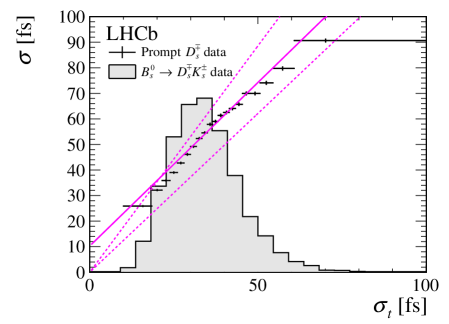
Figure 4: Data points show the measured resolution $\sigma$ as a function of the per-candidate uncertainty $\sigma_{t}$ for prompt $D_{s}^{\mp}$ candidates combined with a random track. The dashed lines indicate the values used to determine the systematic uncertainties on this method. The solid line shows the linear fit to the data as discussed in the text. The histogram overlaid is the distribution of the per-candidate decay-time uncertainty for ${{B}^{0}_{s}}\!\rightarrow D_{s}^{\mp}K^{\pm}$ candidates.

The assumption that the measured decay-time resolution on “fake ${B}^{0}_{s}$” candidates can be used for true ${B}^{0}_{s}$ candidates is justified, as the measured decay-time resolution does not significantly depend on the transverse momentum of the companion particle, which is the main kinematic difference between the samples. In addition, simulation shows that the “fake ${B}^{0}_{s}$” and signal ${B}^{0}_{s}$ samples require compatible correction factors, varying in the range $[1.19,1.27]$.

7 Decay-time acceptance

The decay-time acceptance of ${{B}^{0}_{s}}\!\rightarrow D_{s}^{\mp}K^{\pm}$ candidates is strongly correlated with the $C\!P$ parameters, in particular with ${A_{f}^{\Delta\Gamma}}$ and ${A_{\overline{f}}^{\Delta\Gamma}}$. However, in the case of the flavour-specific ${{B}^{0}_{s}}\!\rightarrow{{D}^{-}_{s}}{{\pi}^{+}}$ decays, the acceptance can be measured by fixing $\Gamma_{s}$ and floating the acceptance parameters. The decay-time acceptance in the ${{B}^{0}_{s}}\!\rightarrow D_{s}^{\mp}K^{\pm}$ fit is fixed to that found in the fit to ${{B}^{0}_{s}}\!\rightarrow{{D}^{-}_{s}}{{\pi}^{+}}$ data, corrected by the acceptance ratio in the two channels obtained from simulation, which is weighted as described in Sec. 4. In all cases, the acceptance is described using segments of cubic b-splines, which are implemented in an analytic way in the decay-time fit [47]. The spline boundaries, knots, are chosen in order to model reliably the features of the acceptance shape, and are placed at $0.5$, $1.0$, $1.5$, $2.0$, $3.0$ and $12.0{\mathrm{\,ps}}$. In the sFit procedure applied to the sample of ${{B}^{0}_{s}}\!\rightarrow{{D}^{-}_{s}}{{\pi}^{+}}$ candidates, the $C\!P$-violation parameter $C_{f}$ is fixed to unity with $C_{f}=-C_{\overline{f}}$, while $S_{f}$, $S_{\overline{f}}$, ${A_{f}^{\Delta\Gamma}}$, and ${A_{\overline{f}}^{\Delta\Gamma}}$ are all fixed to zero. The spline parameters and $\Delta m_{s}$ are free to vary. The result of the sFit procedure applied to the ${{B}^{0}_{s}}\!\rightarrow{{D}^{-}_{s}}{{\pi}^{+}}$ candidates is shown in Fig. 5.

Extensive studies with simulation have been performed and confirm the validity of the method. An alternative analytical decay-time acceptance parametrisation has been considered, and is in good agreement with the nominal spline description. Finally, doubling the number of knots results in negligible changes in the fit result.

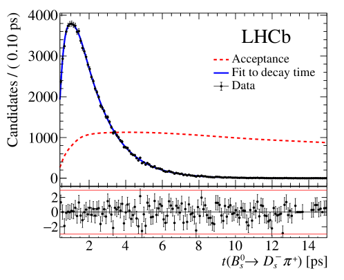
Figure 5: Decay time distribution of ${{B}^{0}_{s}}\!\rightarrow{{D}^{-}_{s}}{{\pi}^{+}}$ candidates obtained by the sPlot technique. The solid blue curve is the result of the sFit procedure and the dashed red curve shows the measured decay-time acceptance in arbitrary units. Normalised residuals are shown underneath.

8 Decay-time fit to ${{B}^{0}_{s}}\!\rightarrow D_{s}^{\mp}K^{\pm}$

In the sFit procedure applied to the ${{B}^{0}_{s}}\!\rightarrow D_{s}^{\mp}K^{\pm}$ candidates, the following parameters

$$\Delta m_{s} =(17.757\pm 0.021){\mathrm{\,ps^{-1}}}\,,$$ (7)

$$\Gamma_{s} =(0.6643\pm 0.0020){\mathrm{\,ps^{-1}}}\,,$$

$$\Delta\Gamma_{s} =(0.083\pm 0.006){\mathrm{\,ps^{-1}}}\,,$$

$$\rho({\Gamma_{{s}}},{\Delta\Gamma_{{s}}}) =-0.239\,,$$

$$A_{\textrm{prod}} =(1.1\pm 2.7)\%,$$

$$A_{\textrm{det}} =(1\pm 1)\%$$

are fixed to their central values. The values of ${B}^{0}_{s}$ oscillation frequency and production asymmetry, $A_{\rm prod}$, are based on LHCb measurements  [48, 49]. The ${B}^{0}_{s}$ decay width, $\Gamma_{s}$, the decay-width difference, $\Delta\Gamma_{s}$, and their correlation, $\rho({\Gamma_{{s}}},{\Delta\Gamma_{{s}}})$, correspond to the HFLAV [15] world average. An estimate of the detection asymmetry $A_{\textrm{det}}$ based on Ref. [50] is considered. The production asymmetry is defined as $A_{\textrm{prod}}\equiv[\sigma({{\kern 1.79993pt\overline{\kern-1.79993ptB}{}}{}^{0}_{s}})-\sigma({{B}^{0}_{s}})]/[\sigma({{\kern 1.79993pt\overline{\kern-1.79993ptB}{}}{}^{0}_{s}})+\sigma({{B}^{0}_{s}})]$, where $\sigma$ denotes the production cross-section inside the LHCb acceptance. The detection asymmetry is defined as the difference in reconstruction efficiency between the ${{D}^{-}_{s}}K^{+}$ and the ${{D}^{+}_{s}}K^{-}$ final states. The detection and the production asymmetries contribute to the PDF with factors of $(1\pm A_{\textrm{prod}})$ and $(1\pm A_{\textrm{det}})$, depending on the tagged initial state and the reconstructed final state, respectively. The tagging calibration parameters and asymmetries are allowed to float within Gaussian constraints based on their statistical and systematic uncertainties given in Sec. 5. The decay-time PDF is convolved with a single Gaussian representing the per-candidate decay-time resolution, and multiplied by the decay-time acceptance described in Sec. 6 and Sec. 7, respectively.

The measured $C\!P$-violating parameters are given in Table 3, and the correlations of their statistical uncertainties are given in Table 4. The fit to the decay-time distribution is shown in Fig. 6. together with the two decay-time-dependent asymmetries, $A_{\rm mix}(D^{+}_{s}K^{-})$ and $A_{\rm mix}(D^{-}_{s}K^{+})$, that are defined as the difference of the decay rates (see Eqs. 1 and 2) of the tagged candidates. The asymmetries are obtained by folding the decay time in one mixing period $2\pi/\Delta m_{s}$. The central values of the $C\!P$ parameters measured by the fit are used to determine the plotted asymmetries.

Table 3: Values of the $C\!P$-violation parameters obtained from the fit to the decay-time distribution of ${{B}^{0}_{s}}\!\rightarrow D_{s}^{\mp}K^{\pm}$ decays. The first uncertainty is statistical and the second is systematic.

Parameter	Value
$C_{f}$	$\phantom{+}0.730\pm 0.142\pm 0.045$
${A_{f}^{\Delta\Gamma}}$	$\phantom{+}0.387\pm 0.277\pm 0.153$
${A_{\overline{f}}^{\Delta\Gamma}}$	$\phantom{+}0.308\pm 0.275\pm 0.152$
$S_{f}$	$-0.519\pm 0.202\pm 0.070$
$S_{\overline{f}}$	$-0.489\pm 0.196\pm 0.068$

Table 4: Statistical correlation matrix of the $C\!P$ parameters. Other fit parameters have negligible correlations with the $C\!P$ parameters.

Parameter	$C_{f}$	${A_{f}^{\Delta\Gamma}}$	${A_{\overline{f}}^{\Delta\Gamma}}$	$S_{f}$	$S_{\overline{f}}$
$C_{f}$	$\phantom{+}1$	$\phantom{+}0.092$	$\phantom{+}0.078$	$\phantom{+}0.008$	$-0.057$
${A_{f}^{\Delta\Gamma}}$		$\phantom{+}1$	$\phantom{+}0.513$	$-0.083$	$-0.004$
${A_{\overline{f}}^{\Delta\Gamma}}$			$\phantom{+}1$	$-0.042$	$-0.003$
$S_{f}$				$\phantom{+}1$	$\phantom{+}0.001$
$S_{\overline{f}}$					$\phantom{+}1$

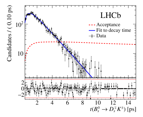
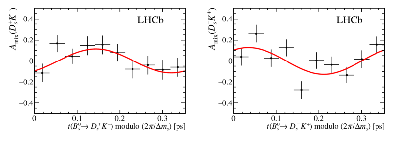
Figure 6: The (top) decay-time distribution of ${{B}^{0}_{s}}\!\rightarrow D_{s}^{\mp}K^{\pm}$ candidates obtained by the sPlot technique. The solid blue curve is the result of the sFit procedure and the dashed red curve shows the decay-time acceptance in arbitrary units, obtained from the sFit procedure applied to the ${{B}^{0}_{s}}\!\rightarrow{{D}^{-}_{s}}{{\pi}^{+}}$ candidates and corrected for the ratio of decay-time acceptances of ${{B}^{0}_{s}}\!\rightarrow D_{s}^{\mp}K^{\pm}$ and ${{B}^{0}_{s}}\!\rightarrow{{D}^{-}_{s}}{{\pi}^{+}}$ from simulation. Normalised residuals are shown underneath. The $C\!P$-asymmetry plots for (bottom left) the ${{D}^{+}_{s}}K^{-}$ final state and (bottom right) the ${{D}^{-}_{s}}K^{+}$ final state, folded into one mixing period $2\pi/\Delta m_{s}$, are also shown.

9 Systematic uncertainties

Systematic uncertainties arise from the fixed parameters $\Delta m_{s}$, $\Gamma_{s}$, $\Delta\Gamma_{s}$,  the detection $A_{\rm det}$ and tagging efficiency $\Delta{\varepsilon_{\mathrm{tag}}}$ asymmetries, and from the limited knowledge of the decay-time resolution and acceptance. In addition, the impact of neglecting correlations among the observables for background candidates is estimated. Table 5 summarises the different contributions to the systematic uncertainties, which are detailed below.

The systematic uncertainties are estimated using large sets of pseudoexperiments, in which the relevant parameters are varied. The pseudoexperiments are generated with central values of the $C\!P$ parameters reported in Sec. 8. They are subsequently processed by the same fit procedure applied to data. The fitted values are compared between the nominal fit, where all fixed parameters are kept at their nominal values, and the systematic fit, where each parameter is varied according to its uncertainty. A distribution is formed by normalising the resulting differences to the uncertainties measured in the nominal fit, and the mean and width of this distribution are added in quadrature and assigned as the systematic uncertainty.

The systematic uncertainty related to the decay-time resolution model, together with its impact on the flavour tagging, is evaluated by fitting the ${{B}^{0}_{s}}\!\rightarrow D_{s}^{\mp}K^{\pm}$ pseudoexperiments using the two alternative decay-time resolution models and their corresponding tagging calibration parameters. The latter are obtained with ${{B}^{0}_{s}}\!\rightarrow{{D}^{-}_{s}}{{\pi}^{+}}$ pseudoexperiments that were generated with the nominal decay-time resolution, but fitted with the two alternative decay-time resolution models.

Table 5: Systematic uncertainties on the $C\!P$ parameters, relative to the statistical uncertainties.

Source	$C_{f}$	${A_{f}^{\Delta\Gamma}}$	${A_{\overline{f}}^{\Delta\Gamma}}$	$S_{f}$	$S_{\overline{f}}$
Detection asymmetry	0.02	0.28	0.29	0.02	0.02
$\Delta m_{s}$	0.11	0.02	0.02	0.20	0.20
Tagging and scale factor	0.18	0.02	0.02	0.16	0.18
Tagging asymmetry	0.02	0.00	0.00	0.02	0.02
Correlation among observables	0.20	0.38	0.38	0.20	0.18
Closure test	0.13	0.19	0.19	0.12	0.12
Acceptance, simulation ratio	0.01	0.10	0.10	0.01	0.01
Acceptance data fit, $\Gamma_{{s}}$, $\Delta\Gamma_{{s}}$	0.01	0.18	0.17	0.00	0.00
Total	0.32	0.55	0.55	0.35	0.35

The impact of neglecting the correlations among the observables in the background is accounted for by means of a dedicated set of pseudoexperiments in which the correlations are included at generation and neglected in the fit. The correlations between $\Gamma_{{s}}$, $\Delta\Gamma_{{s}}$, and the decay-time acceptance parameters from the fit to ${{B}^{0}_{s}}\!\rightarrow{{D}^{-}_{s}}{{\pi}^{+}}$ data are accounted for by fitting pseudoexperiments, where the values of the spline coefficients, $\Gamma_{{s}}$ and $\Delta\Gamma_{{s}}$ are randomly generated according to multidimensional correlated Gaussian distributions centred at the nominal values. The combined correlated systematic uncertainty is listed as “acceptance data fit, $\Gamma_{{s}}$, $\Delta\Gamma_{{s}}$”. The correlations between the spline coefficients among ${{B}^{0}_{s}}\!\rightarrow{{D}^{-}_{s}}{{\pi}^{+}}$ and ${{B}^{0}_{s}}\!\rightarrow D_{s}^{\mp}K^{\pm}$ simulation samples are accounted for by fitting pseudoexperiments with the parameters randomly generated as in the previous case, and the corresponding systematic uncertainty is listed as “acceptance, simulation ratio”.

Table 6: Correlation matrix of the total systematic uncertainties of the $C\!P$ parameters.

Parameter	$C_{f}$	${A_{f}^{\Delta\Gamma}}$	${A_{\overline{f}}^{\Delta\Gamma}}$	$S_{f}$	$S_{\overline{f}}$
$C_{f}$	$\phantom{+}1$	$\phantom{+}0.05$	$\phantom{+}0.03$	$\phantom{+}0.03$	$-0.01$
${A_{f}^{\Delta\Gamma}}$		$\phantom{+}1$	$\phantom{+}0.42$	$0.02$	$0.02$
${A_{\overline{f}}^{\Delta\Gamma}}$			$\phantom{+}1$	$0.03$	$0.03$
$S_{f}$				$\phantom{+}1$	$\phantom{+}0.01$
$S_{\overline{f}}$					$\phantom{+}1$

The nominal result is cross-checked by splitting the sample into subsets according to the two magnet polarities, the year of data taking, the ${B}^{0}_{s}$ momentum, and the BDTG response. No dependencies are observed. In particular, the compatibility of the 1$\mbox{\,fb}^{-1}$ and the 2$\mbox{\,fb}^{-1}$ subsamples is at the level of 1 $\sigma$, where $\sigma$ is the standard deviation. A closure test using the high-statistics fully simulated signal candidates provides an estimate of the intrinsic uncertainty related to the fit procedure. No bias is found and only the fit uncertainty is considered as a systematic uncertainty. The systematic effects due to the background subtraction in the sFit procedure are checked. Therefore, the nominal fitting procedure is applied to a mixture of the signal and the ${{B}^{0}_{s}}\!\rightarrow{{D}^{-}_{s}}{{\pi}^{+}}$ simulation samples as well as combinatorial background data. The result is consistent with the values found by the fit to the signal only, as a consequence, no additional uncertainties are considered.

The resulting systematic uncertainties are shown in Table 5 relative to the corresponding statistical uncertainties. The total systematic correlation matrix, reported in Table 6, is obtained by adding the covariance matrices corresponding to each source.

A number of other possible systematic effects are studied, but found to be negligible. These include production asymmetries, missing or imperfectly modelled backgrounds, and fixed signal-shape parameters in the multivariate fit. Potential systematic effects due to fixed background yields are evaluated by generating pseudoexperiments with the nominal value for these yields, and fitting back with the yields fixed to twice or half their nominal value. No significant bias is observed and no systematic uncertainty assigned. The decay-time fit is repeated adding one or two additional spline functions to the decay-time acceptance description and no significant change in the fit result is observed. The multivariate and decay-time fits are repeated randomly removing multiple candidates, with no significant change observed in the fit result. No systematic uncertainty is assigned to the imperfect knowledge of the momentum and the longitudinal dimension of the detector since both effects are taken into account by the systematic uncertainty on $\Delta m_{s}$, as the world average is dominated by the LHCb measurement [48].

10 Interpretation

The measurement of the $C\!P$ parameters is used to determine the values of $\gamma-2\beta_{s}$ and, subsequently, of the angle $\gamma$. The following likelihood is maximised, replicating the procedure described in Ref. [6],

$$\mathcal{L}(\vec{\alpha})=\exp\left(-\frac{1}{2}\left(\vec{A}(\vec{\alpha})-\vec{A}_{\text{obs}}\right)^{T}V^{-1}\left(\vec{A}(\vec{\alpha})-\vec{A}_{\text{obs}}\right)\right)\,,$$ (8)

where $\vec{\alpha}=(\gamma,\beta_{s},r_{D_{s}K},\delta)$ is the vector of the physics parameters, $\vec{A}(\vec{\alpha})$ is the vector of parameters expressed through Eq. 5, $\vec{A}_{\text{obs}}$ is the vector of the measured $C\!P$-violating parameters and $V$ is the experimental (statistical and systematic) uncertainty covariance matrix. Confidence intervals are computed by evaluating the test statistic $\Delta\chi^{2}\equiv\chi^{2}(\vec{\alpha}^{\prime}_{\min})-\chi^{2}(\vec{\alpha}_{\min})$, where $\chi^{2}(\vec{\alpha})=-2\ln\mathcal{L}(\vec{\alpha})$, following Ref. [51]. Here, $\vec{\alpha}_{\min}$ denotes the global maximum of Eq. 8, and $\vec{\alpha}^{\prime}_{\min}$ is the conditional maximum when the parameter of interest is fixed to the tested value.

The value of $\beta_{s}$ is constrained to the value obtained from [15], ${\phi_{{s}}}=-0.030\pm 0.033\mathrm{\,rad}$, assuming ${\phi_{{s}}}=-2\beta_{s}$, i.e. neglecting contributions from penguin-loop diagrams or from processes beyond the SM. The results are

$$\gamma =(128\,_{-22}^{+17})^{\circ}\,,$$

$$\delta =(358\,_{-14}^{+13})^{\circ}\,,$$

$$r_{D_{s}K} =0.37\,_{-0.09}^{+0.10}\,,$$

where the values for the angles are expressed modulo $180^{\circ}$. Figure 7 shows the $1-\textrm{CL}$ curve for $\gamma$, and the two-dimensional contours of the profile likelihood $\mathcal{L}(\vec{\alpha}^{\prime}_{\min})$.

The resulting value of $\gamma$ is visualised in Fig. 7 by inspecting the complex plane for the measured amplitude coefficients. The points determined by $(-{A_{f}^{\Delta\Gamma}},S_{f})$ and $(-{A_{\overline{f}}^{\Delta\Gamma}},S_{\overline{f}})$ are proportional to $r_{D_{s}K}e^{i(\pm\delta-(\gamma-2\beta_{s}))}$, whilst an additional constraint on $r_{D_{s}K}$ arises from $C_{f}$. The value of $\gamma$ measured in this analysis is compatible at the level of $2.3\,\sigma$, where $\sigma$ is the standard deviation, with the value of $\gamma$ found from the combination of all LHCb measurements [6] when all information from ${{B}^{0}_{s}}\!\rightarrow D_{s}^{\mp}K^{\pm}$ decays is removed. The observed change in the fit log-likelihood between the combined best fit point and the origin in the complex plane indicates $3.8\,\sigma$ evidence for $C\!P$ violation in ${{B}^{0}_{s}}\rightarrow{{D}^{\mp}_{s}}{{K}^{\pm}}$.

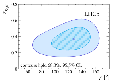
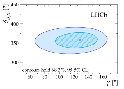
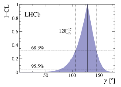
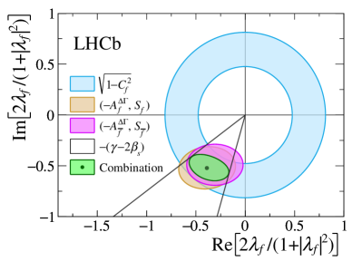
Figure 7: Profile likelihood contours of (top left) $r_{D_{s}K}$ vs. $\gamma$, and (top right) $\delta$ vs. $\gamma$. The markers denote the best-fit values. The contours correspond to 68.3% CL (95.5% CL). The graph on the bottom left shows $1-{\rm CL}$ for the angle $\gamma$, together with the central value and the 68.3% CL interval as obtained from the frequentist method described in the text. The bottom right plot shows a visualisation of how each of the amplitude coefficients contributes towards the overall constraint on the weak phase, $\gamma-2\beta_{s}$. The difference between the phase of $(-{A_{f}^{\Delta\Gamma}},S_{f})$ and $(-{A_{\overline{f}}^{\Delta\Gamma}},S_{\overline{f}})$ is proportional to the strong phase $\delta$, which is close to $360^{\circ}$ and thus not indicated in the figure.

11 Conclusion

The $C\!P$-violating parameters that describe the ${{B}^{0}_{s}}\!\rightarrow D_{s}^{\mp}K^{\pm}$ decay rates have been measured using a data set corresponding to an integrated luminosity of $3.0\mbox{\,fb}^{-1}$ of $pp$ collisions recorded with the LHCb detector. Their values are found to be

$$C_{f} =\phantom{-}0.73\pm 0.14\pm 0.05\,,$$

$${A_{f}^{\Delta\Gamma}} =\phantom{-}0.39\pm 0.28\pm 0.15\,,$$

$${A_{\overline{f}}^{\Delta\Gamma}} =\phantom{-}0.31\pm 0.28\pm 0.15\,,$$

$$S_{f} =-0.52\pm 0.20\pm 0.07\,,$$

$$S_{\overline{f}} =-0.49\pm 0.20\pm 0.07\,,$$

where the first uncertainties are statistical and the second are systematic. The results are used to determine the CKM angle $\gamma$, the strong-phase difference $\delta$ and the amplitude ratio $r_{D_{s}K}$ between the $B^{0}_{s}\rightarrow D_{s}^{-}K^{+}$ and ${{\kern 1.79993pt\overline{\kern-1.79993ptB}{}}{}^{0}_{s}}\rightarrow D_{s}^{-}K^{+}$ amplitudes leading to $\gamma=(128\,_{-22}^{+17})^{\circ}$, $\delta=(358\,^{+13}_{-14})^{\circ}$ and $r_{D_{s}K}=0.37\,^{+0.10}_{-0.09}$ (all angles are given modulo $180^{\circ}$). This result corresponds to $3.8\,\sigma$ evidence of $C\!P$ violation in this channel and represents the most precise determination of $\gamma$ from ${B}^{0}_{s}$ meson decays.

References

- [1] N. Cabibbo, Unitary symmetry and leptonic decays, Phys. Rev. Lett. 10 (1963) 531
- [2] M. Kobayashi and T. Maskawa, violation in the renormalizable theory of weak interaction, Prog. Theor. Phys. 49 (1973) 652
- [3] C. Jarlskog, Commutator of the quark mass matrices in the standard electroweak model and a measure of maximal nonconservation, Phys. Rev. Lett. 55 (1985) 1039
- [4] R. Huerta and R. Pérez-Marcial, Comment on ”commutator of the quark mass matrices in the standard electroweak model and a measure of maximal nonconservation.”, Phys. Rev. Lett. 58 (1987) 1698
- [5] C. Jarlskog, Jarlskog responds, Phys. Rev. Lett. 57 (1986) 2875
- [6] LHCb collaboration, R. Aaij et al., Measurement of the CKM angle from a combination of LHCb results, JHEP 12 (2016) 087, arXiv:1611.03076
- [7] I. Dunietz and R. G. Sachs, Asymmetry between inclusive charmed and anticharmed modes in , decay as a measure of violation, Phys. Rev. D37 (1988) 3186, Erratum ibid. D39 (1989) 3515
- [8] R. Aleksan, I. Dunietz, and B. Kayser, Determining the CP violating phase , Z. Phys. C54 (1992) 653
- [9] R. Fleischer, New strategies to obtain insights into CP violation through , , … and , , … decays, Nucl. Phys. B671 (2003) 459, arXiv:hep-ph/0304027
- [10] K. De Bruyn et al., Exploring decays in the presence of a sizable width difference , Nucl. Phys. B868 (2013) 351, arXiv:1208.6463
- [11] BaBar collaboration, B. Aubert et al., Measurement of time-dependent CP-violating asymmetries and constraints on with partial reconstruction of decays, Phys. Rev. D71 (2005) 112003, arXiv:hep-ex/0504035
- [12] BaBar collaboration, B. Aubert et al., Measurement of time-dependent CP asymmetries in and decays, Phys. Rev. D73 (2006) 111101, arXiv:hep-ex/0602049
- [13] Belle collaboration, F. J. Ronga et al., Measurement of violation in and decays, Phys. Rev. D73 (2006) 092003, arXiv:hep-ex/0604013
- [14] Belle collaboration, S. Bahinipati et al., Measurements of time-dependent CP asymmetries in decays using a partial reconstruction technique, Phys. Rev. D84 (2011) 021101, arXiv:1102.0888
- [15] Heavy Flavor Averaging Group, Y. Amhis et al., Averages of -hadron, -hadron, and -lepton properties as of Summer 2014, arXiv:1412.7515, updated results at Spring 2016 and plots available at http://www.slac.stanford.edu/xorg/hflav/
- [16] L. Wolfenstein, Parametrization of the Kobayashi-Maskawa matrix, Phys. Rev. Lett. 51 (1983) 1945
- [17] Particle Data Group, C. Patrignani et al., Review of particle physics, Chin. Phys. C40 (2016) 100001
- [18] LHCb collaboration, R. Aaij et al., Measurement of violation and the meson decay width difference with and decays, Phys. Rev. D87 (2013) 112010, arXiv:1304.2600
- [19] LHCb collaboration, R. Aaij et al., Measurement of asymmetry in decays, JHEP 11 (2014) 060, arXiv:1407.6127
- [20] LHCb collaboration, R. Aaij et al., Measurement of the asymmetry in – mixing, Phys. Rev. Lett. 117 (2016) 061803, arXiv:1605.09768
- [21] M. Pivk and F. R. Le Diberder, sPlot: A statistical tool to unfold data distributions, Nucl. Instrum. Meth. A555 (2005) 356, arXiv:physics/0402083
- [22] Y. Xie, sFit: a method for background subtraction in maximum likelihood fit, arXiv:0905.0724
- [23] LHCb collaboration, A. A. Alves Jr. et al., The LHCb detector at the LHC, JINST 3 (2008) S08005
- [24] LHCb collaboration, R. Aaij et al., LHCb detector performance, Int. J. Mod. Phys. A30 (2015) 1530022, arXiv:1412.6352
- [25] R. Aaij et al., Performance of the LHCb Vertex Locator, JINST 9 (2014) P09007, arXiv:1405.7808
- [26] R. Arink et al., Performance of the LHCb Outer Tracker, JINST 9 (2014) P01002, arXiv:1311.3893
- [27] M. Adinolfi et al., Performance of the LHCb RICH detector at the LHC, Eur. Phys. J. C73 (2013) 2431, arXiv:1211.6759
- [28] R. Aaij et al., The LHCb trigger and its performance in 2011, JINST 8 (2013) P04022, arXiv:1211.3055
- [29] V. V. Gligorov and M. Williams, Efficient, reliable and fast high-level triggering using a bonsai boosted decision tree, JINST 8 (2013) P02013, arXiv:1210.6861
- [30] T. Sjöstrand, S. Mrenna, and P. Skands, A brief introduction to PYTHIA 8.1, Comput. Phys. Commun. 178 (2008) 852, arXiv:0710.3820
- [31] T. Sjöstrand, S. Mrenna, and P. Skands, PYTHIA 6.4 physics and manual, JHEP 05 (2006) 026, arXiv:hep-ph/0603175
- [32] I. Belyaev et al., Handling of the generation of primary events in Gauss, the LHCb simulation framework, J. Phys. Conf. Ser. 331 (2011) 032047
- [33] D. J. Lange, The EvtGen particle decay simulation package, Nucl. Instrum. Meth. A462 (2001) 152
- [34] P. Golonka and Z. Was, PHOTOS Monte Carlo: A precision tool for QED corrections in and decays, Eur. Phys. J. C45 (2006) 97, arXiv:hep-ph/0506026
- [35] Geant4 collaboration, J. Allison et al., Geant4 developments and applications, IEEE Trans. Nucl. Sci. 53 (2006) 270
- [36] Geant4 collaboration, S. Agostinelli et al., Geant4: A simulation toolkit, Nucl. Instrum. Meth. A506 (2003) 250
- [37] M. Clemencic et al., The LHCb simulation application, Gauss: Design, evolution and experience, J. Phys. Conf. Ser. 331 (2011) 032023
- [38] W. D. Hulsbergen, Decay chain fitting with a Kalman filter, Nucl. Instrum. Meth. A552 (2005) 566, arXiv:physics/0503191
- [39] L. Breiman, J. H. Friedman, R. A. Olshen, and C. J. Stone, Classification and regression trees, Wadsworth international group, Belmont, California, USA, 1984
- [40] B. P. Roe et al., Boosted decision trees as an alternative to artificial neural networks for particle identification, Nucl. Instrum. Meth. A543 (2005) 577, arXiv:physics/0408124
- [41] T. Skwarnicki, A study of the radiative cascade transitions between the Upsilon-prime and Upsilon resonances, PhD thesis, Institute of Nuclear Physics, Krakow, 1986, DESY-F31-86-02
- [42] K. S. Cranmer, Kernel estimation in high-energy physics, Comput. Phys. Commun. 136 (2001) 198, arXiv:hep-ex/0011057
- [43] A. Powell et al., Particle identification at LHCb, PoS ICHEP2010 (2010) 020, LHCb-PROC-2011-008
- [44] LHCb collaboration, R. Aaij et al., Neural-network-based same side kaon tagging algorithm calibrated with and decays, JINST 11 (2016) P05010, arXiv:1602.07252
- [45] LHCb collaboration, R. Aaij et al., Opposite-side flavour tagging of mesons at the LHCb experiment, Eur. Phys. J. C72 (2012) 2022, arXiv:1202.4979
- [46] LHCb collaboration, R. Aaij et al., Measurement of violation in decays, Phys. Rev. Lett. 115 (2015) 031601, arXiv:1503.07089
- [47] M. Karbach, G. Raven, and M. Schiller, Decay time integrals in neutral meson mixing and their efficient evaluation, arXiv:1407.0748
- [48] LHCb collaboration, R. Aaij et al., Precision measurement of the – oscillation frequency in the decay , New J. Phys. 15 (2013) 053021, arXiv:1304.4741
- [49] LHCb collaboration, R. Aaij et al., Measurement of the – and – production asymmetries in collisions at , Phys. Lett. B739 (2014) 218, arXiv:1408.0275
- [50] LHCb collaboration, R. Aaij et al., Measurement of asymmetry in and decays, JHEP 07 (2014) 041, arXiv:1405.2797
- [51] LHCb collaboration, R. Aaij et al., A measurement of the CKM angle from a combination of analyses, Phys. Lett. B726 (2013) 151, arXiv:1305.2050
Acknowledgements
We express our gratitude to our colleagues in the CERN accelerator departments for the excellent performance of the LHC. We thank the technical and administrative staff at the LHCb institutes. We acknowledge support from CERN and from the national agencies: CAPES, CNPq, FAPERJ and FINEP (Brazil); MOST and NSFC (China); CNRS/IN2P3 (France); BMBF, DFG and MPG (Germany); INFN (Italy); NWO (The Netherlands); MNiSW and NCN (Poland); MEN/IFA (Romania); MinES and FASO (Russia); MinECo (Spain); SNSF and SER (Switzerland); NASU (Ukraine); STFC (United Kingdom); NSF (USA). We acknowledge the computing resources that are provided by CERN, IN2P3 (France), KIT and DESY (Germany), INFN (Italy), SURF (The Netherlands), PIC (Spain), GridPP (United Kingdom), RRCKI and Yandex LLC (Russia), CSCS (Switzerland), IFIN-HH (Romania), CBPF (Brazil), PL-GRID (Poland) and OSC (USA). We are indebted to the communities behind the multiple open-source software packages on which we depend. Individual groups or members have received support from AvH Foundation (Germany), EPLANET, Marie Skłodowska-Curie Actions and ERC (European Union), ANR, Labex P2IO and OCEVU, and Région Auvergne-Rhône-Alpes (France), RFBR, RSF and Yandex LLC (Russia), GVA, XuntaGal and GENCAT (Spain), Herchel Smith Fund, the Royal Society, the English-Speaking Union and the Leverhulme Trust (United Kingdom).